Article

Construction and Validation of a High-Fidelity Virtual Scene for Low-Stature and High-Biodiversity Ecosystems—Simulating Multi-Modal Sensing Approaches


by
Manisha Das Chaity
*,
Ramesh Bhatta
,
Byron Eng
and
Jan van Aardt
Imaging Science, Rochester Institute of Technology, Rochester, NY 14623, USA
*
Author to whom correspondence should be addressed.
Remote Sens. 2026, 18(16), 2816; https://doi.org/10.3390/rs18162816
Submission received: 17 June 2026 / Revised: 8 August 2026 / Accepted: 19 August 2026 / Published: 20 August 2026

Highlights

What are the main findings?
  • Developed and validated a high-fidelity three-dimensional virtual fynbos ecosystem by integrating field measurements, terrestrial laser scanning, structure-from-motion products, and radiative transfer modeling within the DIRSIG simulation environment.
  • Simulated multispectral, hyperspectral, and LiDAR observations closely matched corresponding field-acquired datasets, demonstrating the realism of the virtual scene for remote sensing applications.
What are the implications of the main findings?
  • The framework enables systematic evaluation of information loss across spectral and spatial scales, helping to identify theoretical limits for plant species discrimination and biodiversity monitoring.
  • The virtual scene provides a scalable platform for assessing the performance of current and future remote sensing systems in structurally complex, species-rich ecosystems where direct field measurements are challenging.

Abstract
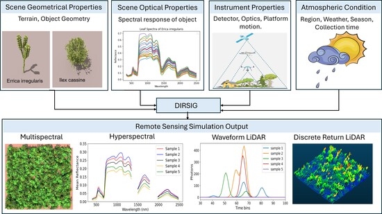
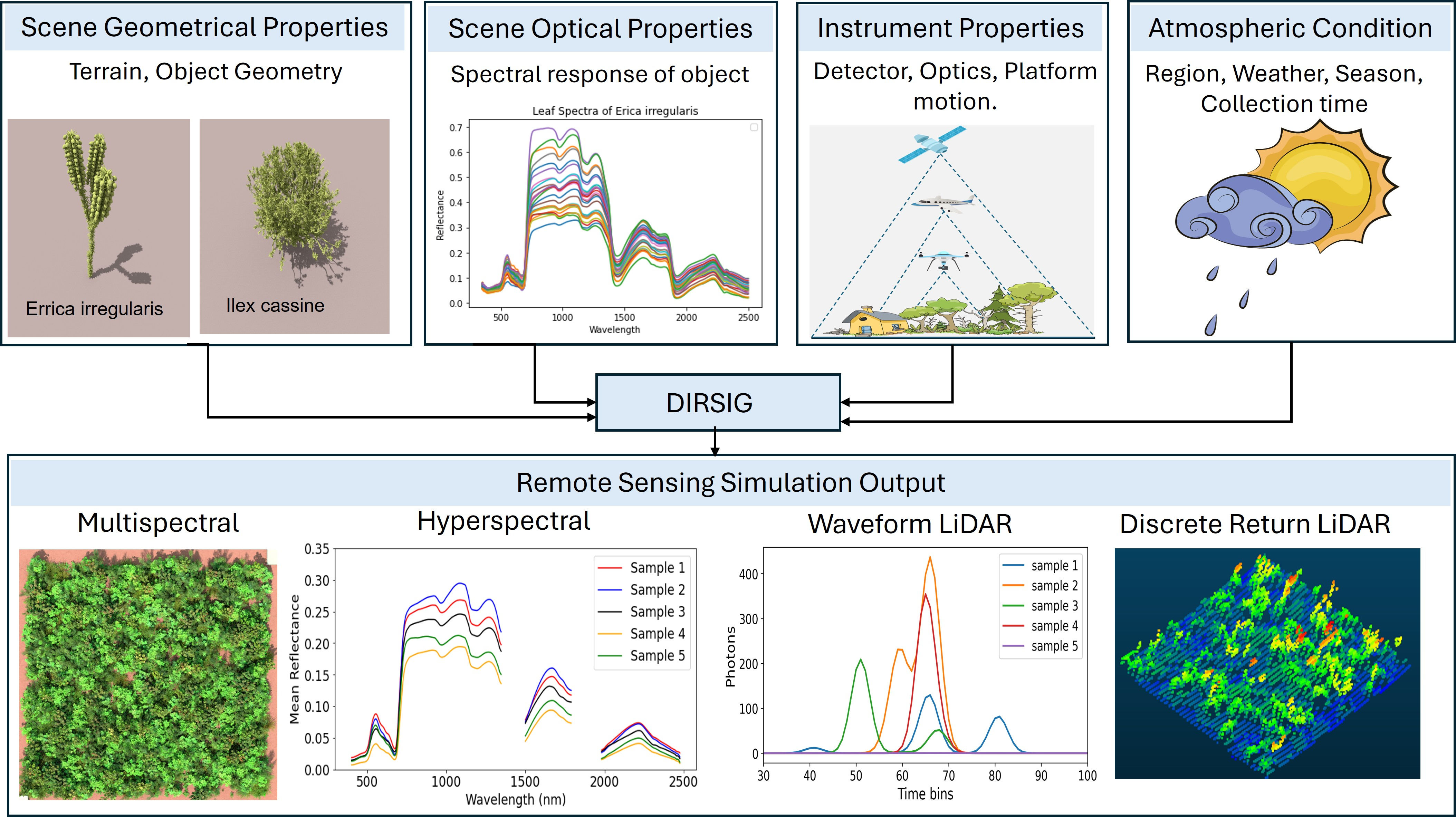
The Greater Cape Floristic Region (GCFR) in South Africa is a fire-prone biodiversity hotspot where high species richness, structural complexity, and small plant sizes (0.0001–4 m2) pose substantial challenges for remote sensing-based biodiversity assessment. Spectral similarity among species and the mismatch between plant size and sensor pixel dimensions limit the capacity of current and forthcoming spaceborne systems to resolve individual species and accurately detect plot-level diversity changes. We therefore developed a physics-based simulation framework that couples fynbos trait measurements with radiative transfer modeling in the DIRSIG (Digital Imaging and Remote Sensing Image Generation) environment towards quantifying information loss across spectral and spatial scales and to define theoretical limits for biodiversity monitoring. We constructed a three-dimensional virtual scene of post-fire fynbos communities in Grootbos Private Nature Reserve, integrating high-resolution imagery, terrestrial laser scanning (TLS), and structure-from-motion (SfM)-derived point clouds. Field measurements of mean diameter and percent cover were used to scale vegetation models and constrain species abundance. We distributed plant instances using a blue noise sampling algorithm, guided by density maps derived from unmanned aerial system (UAS) imagery. Species-specific optical properties were parameterized using field-measured reflectance data and the PROSPECT radiative transfer model, while terrain structure was derived from SfM-based digital terrain models. The integrated scene was used to simulate multispectral (DJI Mavic 3 MSI), hyperspectral (AVIRIS-NG), and light detection and ranging (LiDAR) observations. Agreement between simulated outputs were evaluated against corresponding field-acquired datasets using spectral signatures and vegetation indices. This framework enables systematic assessment of sensor specification effects on spectral biodiversity metrics and provides a pathway for evaluating theoretical limits of species discrimination across airborne and satellite platforms.

Graphical Abstract

1. Introduction

South Africa’s Greater Cape Floristic Region (GCFR) is recognized as a global hotspot of exceptional plant diversity, with approximately 78% of its plant taxa classified as endemic [1]. It encompasses two globally recognized biodiversity hotspots [2], including the fynbos biome, a Mediterranean-type ecosystem characterized by frequent fires. This highly diverse region is increasingly threatened by environmental change, including agricultural expansion, invasive species, modified fire regimes, climate change, and anthropogenic pressures [3,4,5]. Due to high turnover of species in space and time, the GCFR requires sophisticated monitoring and management strategies to mitigate these threats and to map biodiversity of the region, which has drawn the attention of NASA (National Aeronautics and Space Administration) [6] as part of their BioSCape campaign (https://www.bioscape.io/).
Fynbos (“fine bush”), the dominant open shrubland of the GCFR, exhibits a high relative contribution of soils, stems, and other surfaces to observed reflectance. These interactions further increase in complexity due to the exceptionally high ecosystem diversity. Furthermore, fire plays a critical role in shaping the ecosystem and biodiversity of the fynbos biome, influencing vegetation structure, species composition, and nutrient cycling [7,8]. Slingsby et al. [5] and Verboom et al. [9] have reported temporal declines in both species richness and community composition within fynbos vegetation following fire events. Their results suggest that key drivers of these changes include the frequency and intensity of fires, weather conditions during post-fire recovery, and the availability of soil nutrients. Therefore, understanding the evaluation of fynbos sites in terms of the time since last burn is a key aspect of understanding fynbos ecology, as it helps to reveal post-fire succession stages and vegetation recovery patterns.
Species diversity—a fundamental component of biodiversity—is usually quantified through field-based surveys conducted over limited spatial extents. While valuable, these surveys are resource-intensive, requiring considerable time and labor, and they are difficult to scale to larger regions, while being prone to bias and inconsistency [10]. In the GCFR, where species richness and ecological complexity are high, traditional monitoring approaches such as community-level mapping are insufficient [6]. It is in this context that remote sensing offers a powerful alternative, delivering spatially explicit and regularly updated data that are essential for robust and efficient conservation planning.
Recent advances in remote sensing technologies, including imaging spectroscopy (hyperspectral sensing), light detection and ranging (LiDAR), and structure-from-motion (SfM) approaches, have significantly enhanced our ability to characterize fine-scale variation in the taxonomic and functional composition of plant communities across space and time [11]. Spectral diversity metrics derived from hyperspectral data have demonstrated promise in capturing multiple facets of local plant biodiversity [12,13]. Complementarily, LiDAR-based structural metrics—such as vertical foliage distribution and canopy complexity—have shown utility in distinguishing vegetation types and functional assemblages across heterogeneous landscapes [14,15]. More recently, SfM-derived structural metrics have been used to quantify and map species diversity within highly heterogeneous environments, including the fynbos biome of the GCFR [16].
A major limitation of remote sensing in fynbos-type shrublands arises from the mismatch between the coarse spatial resolution of conventional satellite sensors and the highly heterogeneous structure of the vegetation. Sensors such as Landsat and Sentinel-2, with pixel sizes ranging from 10 to 30 m, are unable to resolve the fine-scale spatial variability characteristic of fynbos ecosystems, where individual plants and species patches are often smaller than 1 m [17]. As a result, single pixels frequently contain mixtures of diverse vegetation components, senescent material, bare soil, rocks, and shadows. These “mixed pixels” produce blended spectral signatures that obscure species-level information, reduce classification accuracy, and hinder the detection of rare or endemic species occupying small ecological niches [18]. Consequently, the structural and compositional complexity of fynbos vegetation remains a significant bottleneck for biodiversity mapping using standard satellite remote sensing approaches. These limitations also make it difficult to systematically evaluate how spatial and spectral resolution influence the detectability of biodiversity patterns across heterogeneous landscapes like fynbos.
Rather than relying solely on empirical data, which may be limited in availability or temporal coverage, a more robust strategy involves simulating surface reflectance under a range of biodiversity scenarios grounded in physics-first principles. Such simulations can incorporate observed or hypothetical variations in species richness, functional composition, and structural attributes to predict spectral responses under controlled conditions. We contend that a simulation-based framework—explicitly parameterized with field-informed data on species prevalence, cover (including post-disturbance dynamics), structure, and traits—offers a comprehensive and scalable pathway to elucidating biodiversity–spectral relationships in structurally complex, species-rich ecosystems such as the fynbos.
One-dimensional (1D) radiative transfer models (RTMs) have been widely applied in other South African ecosystems, primarily to generate synthetic datasets that support vegetation classification and mapping efforts [19]. Although effective in certain contexts, these models rely on simplifying assumptions—such as treating surfaces as Lambertian reflectors and vegetation as a turbid medium—which limit their ability to capture the structural complexity of the GCFR. In contrast, three-dimensional (3D) RTMs that employ path-tracing approaches more accurately represent canopy architecture and the intricate interactions of light within heterogeneous vegetation [20]. As a result, 3D RTMs provide a more realistic framework for biodiversity assessment and are particularly valuable for evaluating ecosystem disturbances such as fire and long-term climate change impacts.
Among available 3D radiative transfer environments, DIRSIG (Digital Imaging and Remote Sensing Image Generation) stands out as a physics-based radiometric modeling system designed to generate synthetic remote sensing imagery with radiometric, geometric, and temporal fidelity. It can produce a wide range of datasets—including passive broadband, multispectral, hyperspectral, low-light, polarized, active laser radar, and synthetic aperture radar imagery—through the integration of first-principles-based radiation propagation modules [21,22,23,24,25,26,27]. Recent applications of DIRSIG include assessing the effects of sensor spatial, spectral, and scale resolutions on classification accuracy [28], evaluating the influence of sub-pixel structural heterogeneity on imaging spectrometer responses [29], and developing efficient PAR-based protocols for estimating forest leaf area index (LAI) validated against AVIRIS (Airborne Visible InfraRed Imaging Spectrometer)-derived NDVI [30]. Earlier studies have also employed DIRSIG to investigate the impact of broadleaf tree structure on NEON (National Ecological Observatory Network) Airborne Observation Platform (AOP) waveform LiDAR signals [31], compare deconvolution algorithms [32], evaluate preprocessing workflows [33], reconstruct three-dimensional tree architecture from simulated small-footprint waveform LiDAR data [34], and to model LAI using simulated waveform LiDAR, demonstrating its generalizability to real-world observations [35]. Furthermore, DIRSIG has been instrumental in leveraging LiDAR backscatter phenomenology—first identified through simulations and later confirmed by ground-based structural assessments—to predict coarse woody debris [36] and quantify dense herbaceous biomass in savannas [37]. By adhering to strict physics-based principles, DIRSIG enables robust phenomenological studies, and in this work, we propose to use DIRSIG to model proxies of fynbos field sites across different post-fire ages. Prior DIRSIG applications have primarily targeted structural attributes—such as LAI, biomass, or coarse woody debris—in forested or savanna systems with comparatively low species diversity. In contrast, this study is the first to link field-measured, species-level traits and percent cover directly to physics-based radiative transfer at the individual-plant scale within a hyperdiverse shrubland, enabling controlled, single-variable sensitivity experiments explicitly designed for biodiversity remote sensing rather than structural characterization alone.
We propose that developing a limited number of vegetation types (approximately 10–20) that encompass the dominant species will allow the simulation of realistic reflectance spectra under scenarios spanning a range of taxonomic, functional, and phylogenetic diversity. These simulation scenarios will be developed based on in situ vegetation surveys, field spectroradiometer measurements, and high-resolution unmanned aerial system (UAS) data. The resulting diversity response models subsequently will be validated against imagery acquired during the NASA BioSCape campaign, thereby enabling a robust assessment of the capacity of remote sensing approaches to capture biodiversity patterns in this ecosystem.
This methodological paper outlines our approach to building and validating the study scene. Future goals of this study are to advance understanding of how spectral and structural leaf traits scale from canopy to landscape levels, evaluate their effectiveness as biodiversity indicators, and determine the spatial, spectral, and temporal resolutions necessary for reliably monitoring post-fire recovery and biodiversity change.

2. Materials

2.1. Study Area and Field Data

Our team conducted extensive fieldwork to explore the diverse ecosystems of fynbos in South Africa towards creating a simulated scene under the NASA BioSCape project. We visited the Grootbos Private Nature Reserve in South Africa (see Figure 1) in October 2022 and 2023 to collect field samples. Here, we focused on three plots (Figure 1) in the study area; these plots were selected to capture variability in fynbos species composition and structure, as well as to capture the level of post-fire recovery status based on fire history data. The plots were burned in the years of 2006, 2016, and 2019, where the 2006 plot was 5 × 10 m releves and 2016 and 2019 plots were 5 × 5 m releves. The plot-level data included species identities and estimates of cover, as well as mean diameter and height for all species in each plot. As an example, Table 1 summarizes these data for the 2006 burn year.
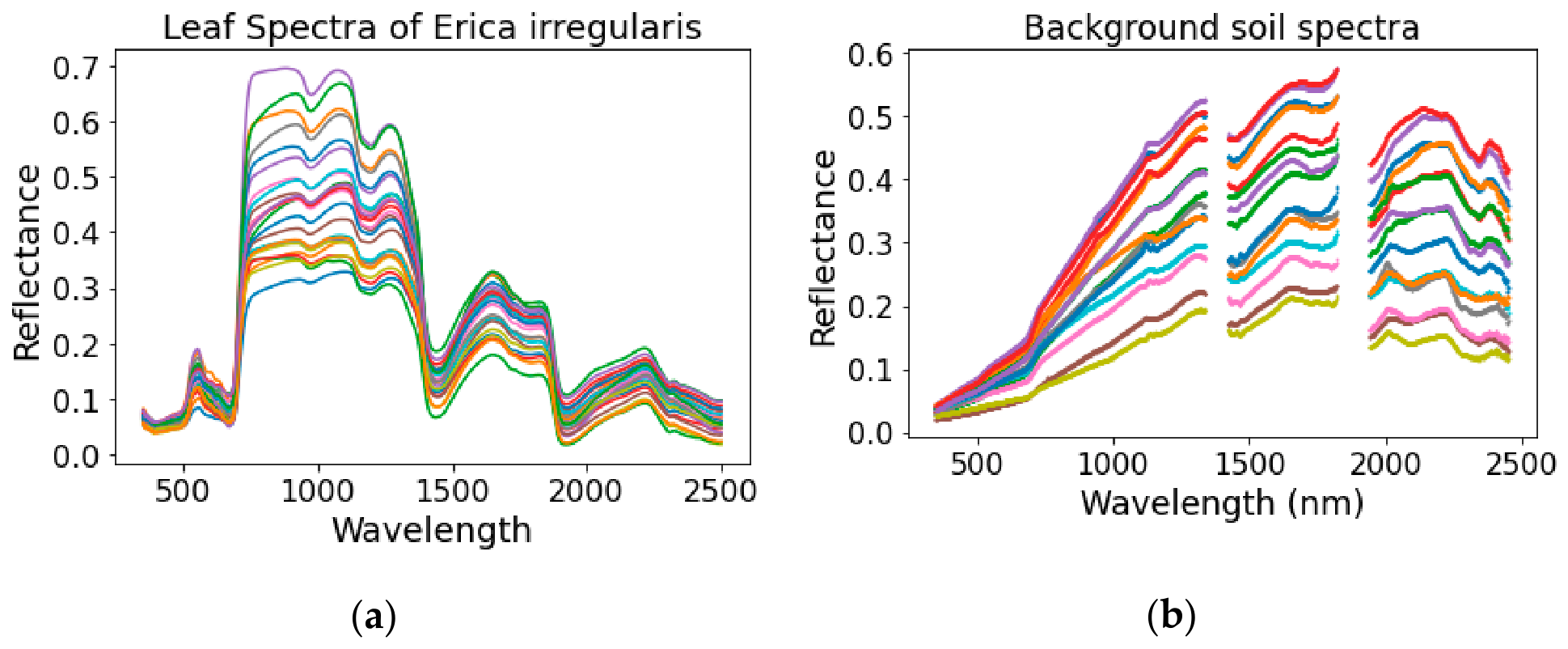
We collected spectral measurements (Figure 2) in the 350–2500 nm range using an Analytical Spectral Devices FieldSpec 3 (ASD) spectroradiometer (ASD Inc., Boulder, CO, USA). Leaf-level measurements of the adaxial surfaces of fine-structured fynbos leaves were captured using a contact probe with a leaf clip. For other targets, including flowers, stems, burned bark, and soil backgrounds (both clean and mixed with charcoal ash), we used an 8° field-of-view (FOV) fore-optic attached to a pistol grip. We used the collected fieldwork data to ensure that we covered the variation in fynbos’ structural and spectral traits across different burned years.

2.2. UAS Data

We acquired multispectral imagery over our study area in the reserve using a DJI Mavic 3 Multispectral UAS (DJI, Shenzhen, China), flown at 50 m above ground level. The platform includes four 5 MP (megapixel) 1/2.8″ CMOS multispectral sensors (green: 560 nm; red: 650 nm; red-edge: 730 nm; NIR: 860 nm) and an additional 20 MP 4/3 CMOS RGB sensor for high-resolution imagery. The resulting ground sampling distance was approximately 2.5 cm per pixel for the multispectral bands. Flights were conducted in October 2023 (spring season) over the same 2006, 2016, and 2019 burn plots where field measurements were collected. Mission planning was based on shapefiles provided by the Grootbos Private Nature Reserve management authority. Structure-from-motion (SfM) data of the UAS imagery produced high-resolution 3D reconstructions of terrain and vegetation structure at the plot scale. These UAS-derived datasets subsequently were used to validate the DIRSIG-simulated imagery. Each flight mission was executed along a predefined grid pattern, maintaining approximately 80% along-track and 70% cross-track overlap to ensure comprehensive spatial coverage. The RGB imagery was processed in Pix4Dmapper (version 4.8.4; Pix4D S.A., Prilly, Switzerland) to produce georeferenced point clouds and high-resolution three-dimensional surface models using a SfM photogrammetric workflow [38,39]. SfM data of the UAS imagery produced high-resolution 3D reconstructions of terrain and vegetation structure at the plot scale. These multimodal UAS-derived datasets subsequently were used in the design of the fynbos scene and to further validate the DIRSIG simulations.

2.3. Additional Data Sources

Supplementary data sources were used to inform both the development of species-specific three-dimensional (3D) models and their spatial configuration within the virtual scene. These resources included high-resolution photographic imagery collected during field campaigns, additional reference images from iNaturalist (https://www.inaturalist.org/), detailed species descriptions from the ecological and botanical literature [40], and regional documentation describing vegetation structure and composition within the GCFR and its fynbos ecosystems (https://www.sanbi.org/). Together, these materials provided essential information on plant morphology, growth form, canopy architecture, and typical spatial associations. This multi-source approach ensured that the virtual representations were ecologically realistic and consistent with observed community patterns characteristic of Mediterranean-type shrubland systems.

3. Methods

3.1. Terrain Building

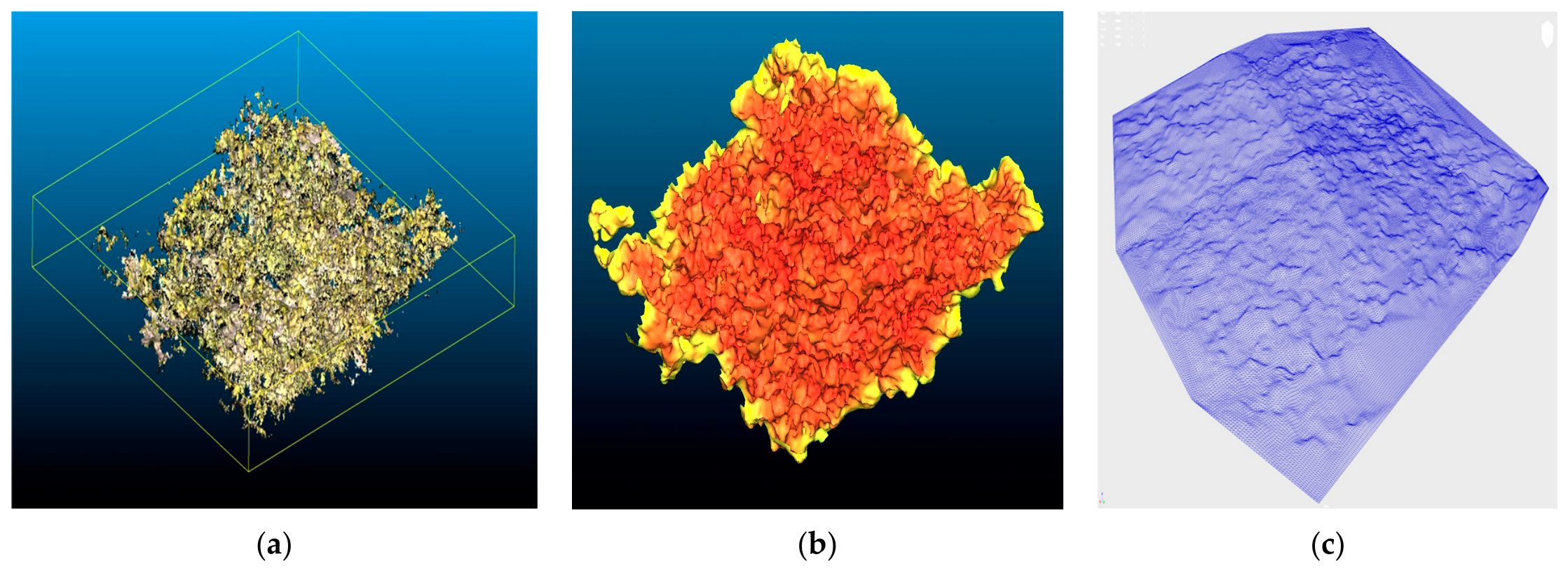
We utilized point clouds, generated from UAS-based SfM data, to construct the base terrain models of various burned plots (Figure 3a). The point clouds were processed in CloudCompare (v2.13 “Kharkiv”, 2024), a 3D visualization and analysis software, where they were converted into faceted 3D meshes suitable for subsequent processing and refinement (Figure 3b). Due to the nature of UAS-based data collection, the resulting point clouds and corresponding faceted meshes contained significant aboveground vegetation, which hindered the integration of simulated or virtual foliage in subsequent modeling workflows. We therefore extracted the lowest elevation points from the dataset representing the ground surface to isolate the terrain and used this as a reference to guide manual retopology. A new terrain mesh was constructed in Autodesk Maya 2024 (Autodesk, Inc., San Francisco, CA, USA) using standard 3D modeling techniques. The original mesh was retained as a locked baseline to preserve accurate ground elevation. Tools such as Quad Draw and Smooth Sculpting brushes were employed to reconstruct gaps corresponding to occluded or vegetated areas in a non-destructive manner, following standard retopology workflows described in the Maya documentation. This process produced a clean terrain mesh that preserved essential ground surface characteristics, while removing unwanted vegetation artifacts from the original dataset (Figure 3c).

3.2. Scene Building Details

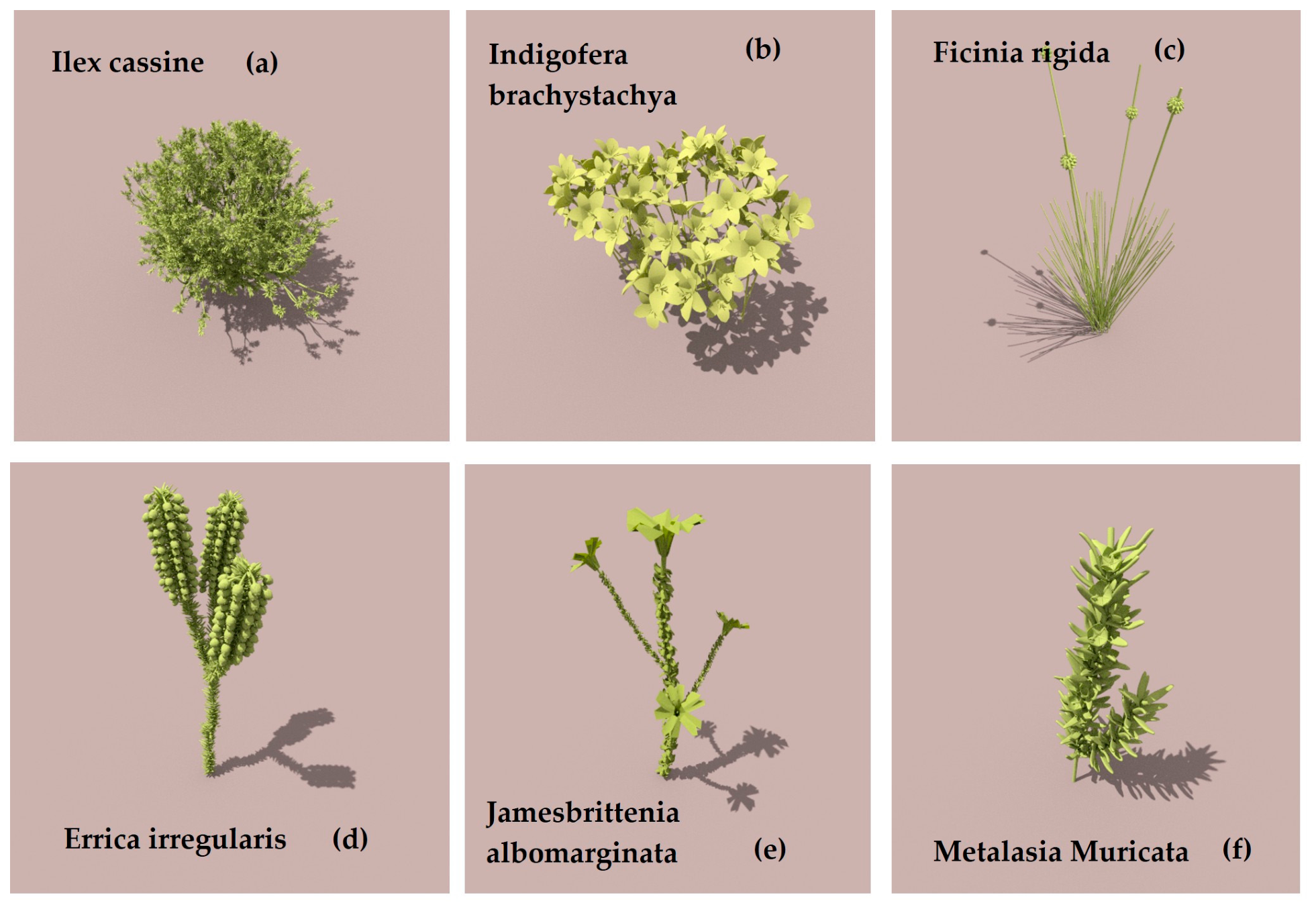
We initially integrated multiple complementary data sources, as described in Section 2.3, to construct realistic three-dimensional (3D) models of representative fynbos plant species (Figure 4). These sources informed key structural attributes—including plant morphology, canopy architecture, and branching patterns—thereby ensuring ecological fidelity in the virtual representations. The resulting 3D models were classified into two categories, namely full-plant models (e.g., Figure 4a–c) and branch-level models (e.g., Figure 4d–f). Branch-level models were instanced multiple times within the simulation environment to approximate the structural appearance of full plants.
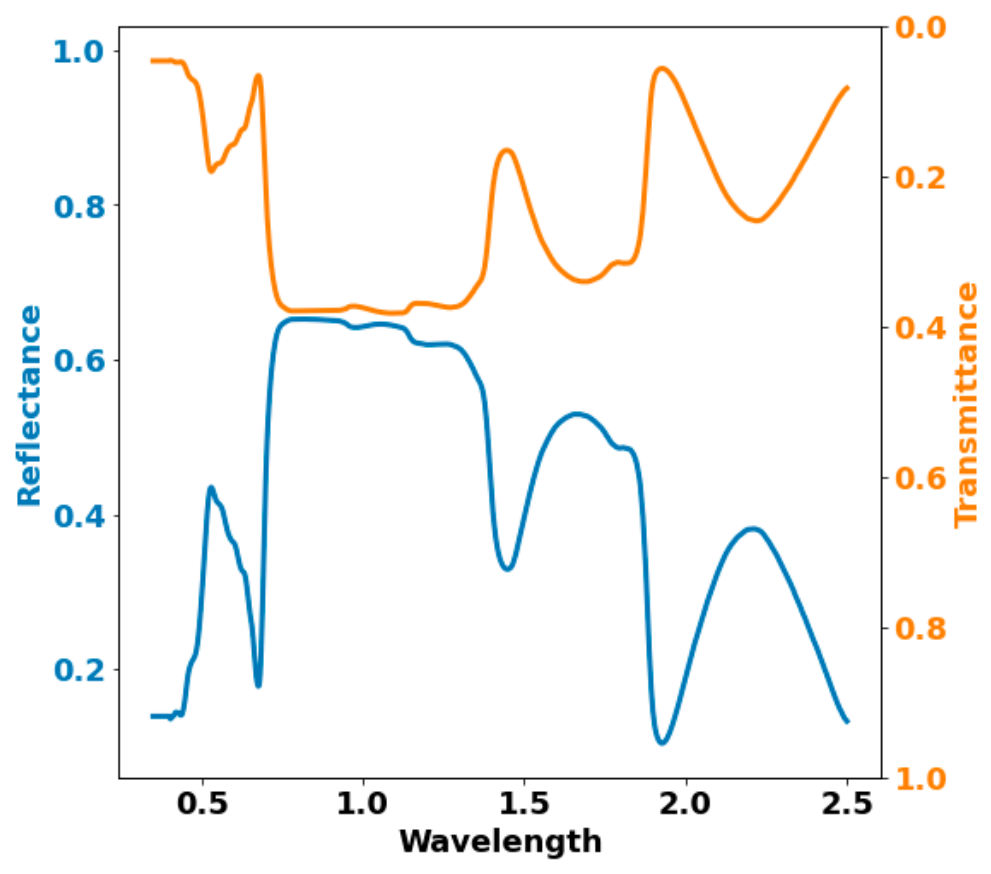
For scene optical properties, we incorporated spectral reflectance and transmittance data obtained from field measurements for each facet, utilizing material IDs. We used different spectral samples, collected for each species, and fitted parameters to a modified PROSPECT model [41] to obtain the transmittance curve for varying spectra (Figure 5). This allowed us to represent different material variants for each species. The underlying terrain was generated using point clouds of the UAS-derived SfM data, as explained in the previous subsection.

3.3. Species Instantiation

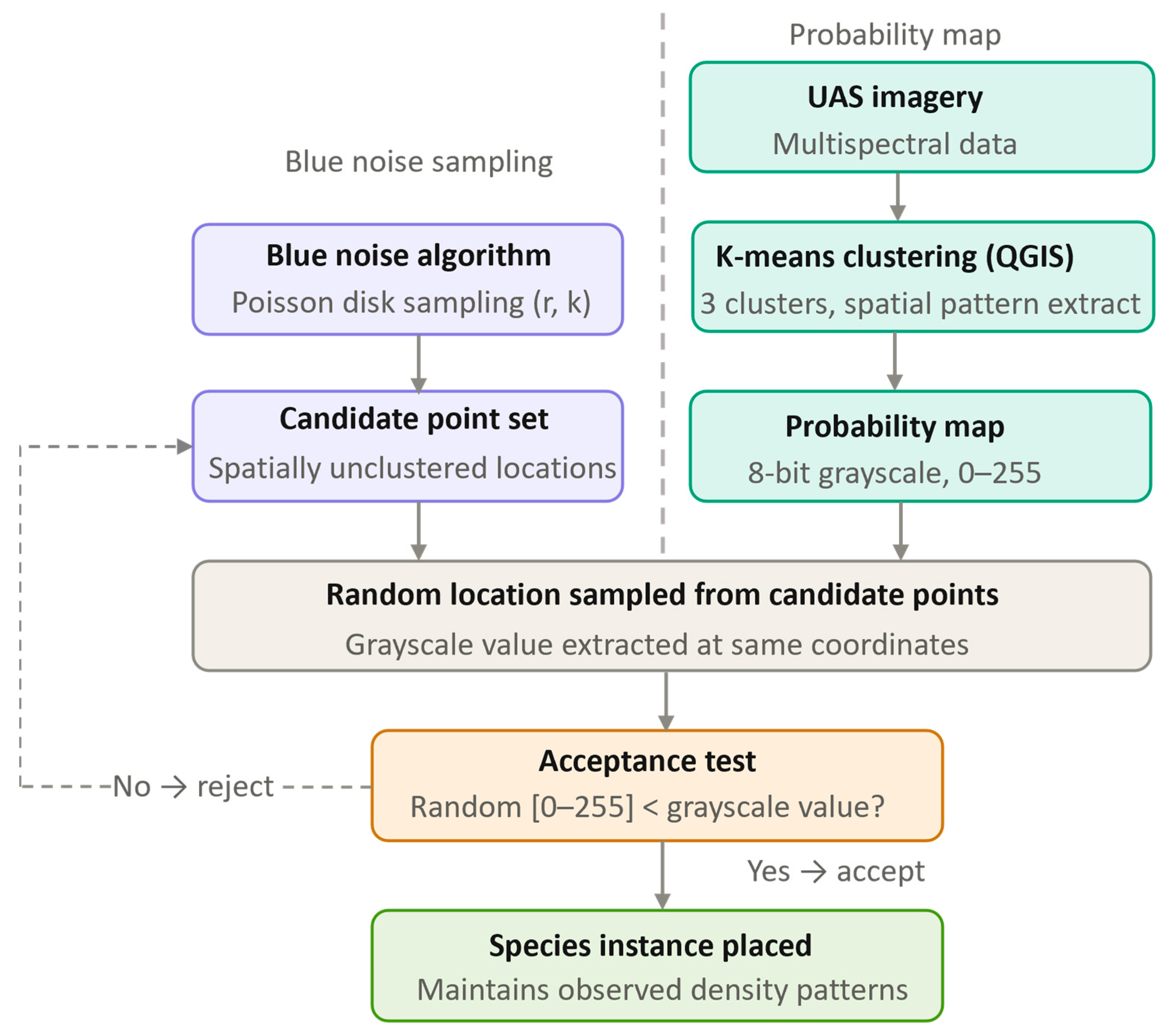
The next step required us to distribute the species throughout the scene in a random manner that maintains realistic spatial distribution patterns. The corresponding workflow is shown in Figure 6. At first, we generated a single blue noise point set for the entire scene, which served as the common sampling space for all species. The blue noise point set was generated using a blue noise algorithm [42] that utilizes Poisson disk sampling, in conjunction with a probability map derived from UAS imagery captured in the study area to achieve this. The results are a statistically uniform mixing of the distribution of species placed throughout the scene in a way that maintained observed density patterns.
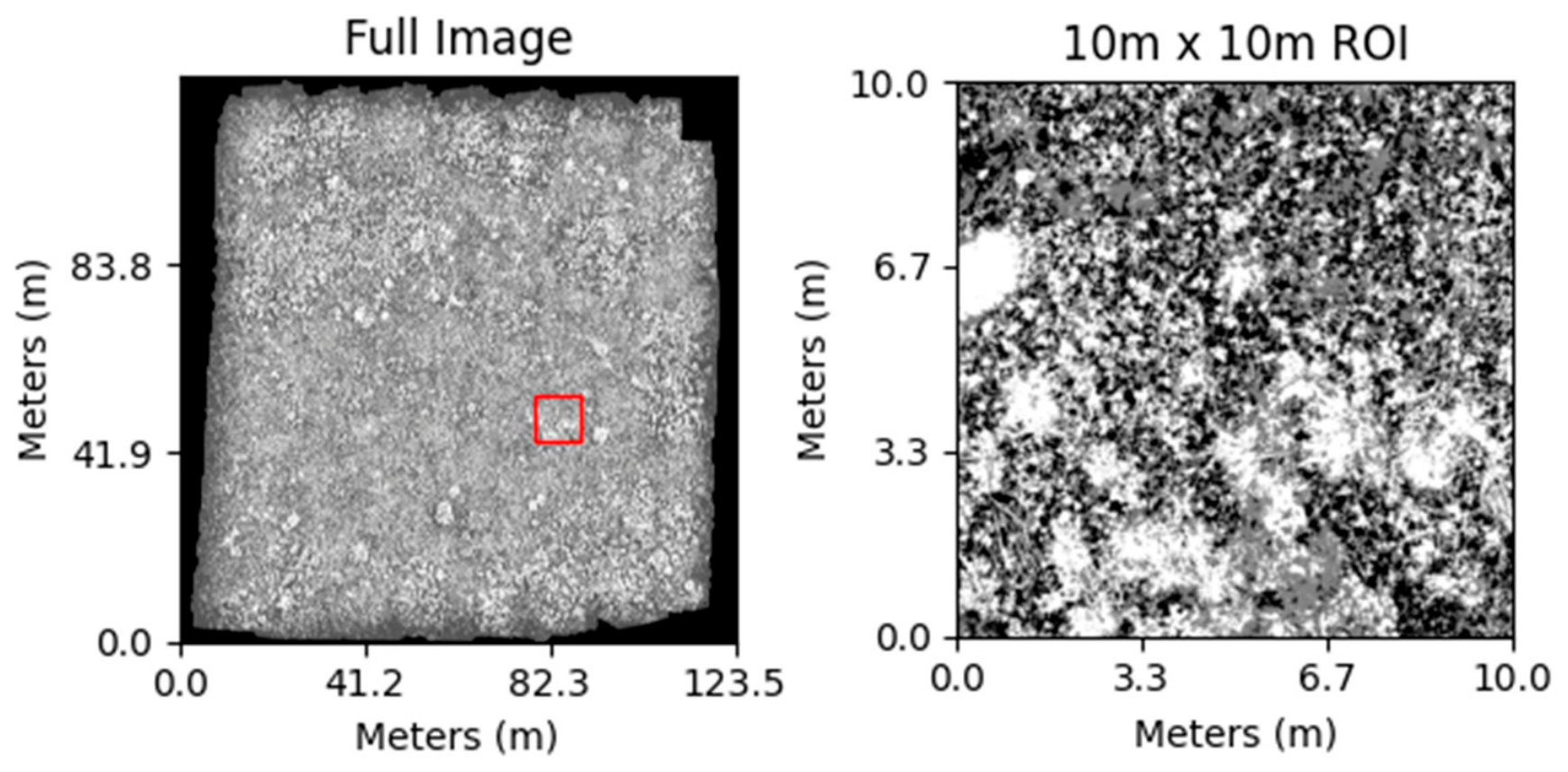
The blue noise algorithm uses the parameters r (minimum distance between points) and k (number of candidates neighboring points around each point). The algorithm recursively generates new points from an initial point until the area is filled and no new points can be added that fit the criteria given by r and k. This creates a randomized, spatially unclustered distribution of points that maintains realistic ecological dispersion pattern [43]. The probability map was created in QGIS by applying a K-means clustering function to the multispectral UAS imagery collected in the area (Figure 7). The function was run with a target of three clusters. While this function is typically used for classification purposes, we used it only to extract spatial patterns from the area. The resulting clusters were not interpreted as ecological classes or used to distinguish species, vegetation density, or cover fractions. Instead, they were used solely to define the spatial probability of vegetation occurrence, while species composition and percent cover were independently prescribed from field measurements during scene parameterization. The resulting map contained the values 0–255 when converted to 8-bit grayscale.
Candidate locations were sequentially sampled from the blue noise point set. For each location, the corresponding grayscale value was extracted from the probability map and compared with a randomly generated value between 0 and 255. If the random value was less than the grayscale value, the location was accepted and an instance of the species was placed; otherwise, the location was rejected. This resulted in acceptance probabilities ranging from 0% for pixels with a value of 0 to approximately 50% for pixels with a value of 128, and 100% for pixels with a value of 255. These values controlled only the probability of vegetation placement and were not interpreted as quantitative measures of vegetation cover or species abundance.
Each species was sequentially sampled from the remaining unused points, accepting or rejecting locations according to its probability map until the target number of individuals was reached. Consequently, the blue noise parameters (r and k) controlled the spatial distribution of plant locations, whereas species abundance, determined by percent cover, controlled the number of individuals placed. This formulation treated spatial distribution and species abundance as independent constraints while ensuring that both were satisfied during species placement.
The Poisson Disk Algorithm operated as follows:
  • Input:
  • Width and height: Dimensions of the sample region;
  • r: Minimum distance between points;
  • k: Maximum number of candidates to generate for each active sample before marking it inactive.
  • Outputs:
Samples: A list of samples in a 2-dimensional space that are at least a distance r from each other and distributed uniformly.
  • Initialize a background grid cell:
  • Set cell size a = r/√2;
  • Calculate grid dimensions x and y where x = ⌈width/a⌉, y = ⌈height/a⌉.
  • Select initial sample:
  • Randomly select an initial sample point, p i = 1 , within the sample region (width, height).
  • Add p i = 1 to the sample list and assign it to the active list.
  • Store the cell index, containing the point, p i = 1 in the background grid cell.
  • While there are sample points in the active list do
    • Randomly select a reference sample point p r e f from the active list.
    • For i = 1 to k:
      • Generate a candidate point, p c , within an annulus (between radius r and 2r) around the reference point, p r e f .
      • Check the distance between the candidate point, p c , and the reference point, p r e f :
        • If the distance is less than r, continue to the next candidate.
        • If p c is at least r away from other samples in neighboring cells, add p c to the samples list, mark it active, and assign its index in the cells grid.
      • Exit the candidate generation loop if a valid p c is found.
    3.
    If no valid candidate point is found after k attempts
    • Remove the reference point, p r e f , from the active list.
  • Return the final samples list containing the uniformly spaced points.

3.4. Estimating the Number of Vegetation Instances

To determine the number of vegetation instances required to achieve a specified percent cover within a scene, we computed the total number of objects based on the target area to be filled and the effective area of each object. We began by calculating the total area to be covered. The scene area was computed as scene   area = width   × height .
The desired target cover was based on species-level percent cover values obtained from an ecological vegetation parameter table. The area that each species should occupy was thus
target   area = scene   area × Percentage   cover 100
Each 3D vegetation model used in the instance placement procedure was represented by its axis-aligned bounding box. The bounding box defined the minimal rectangular prism that fully encloses the 3D geometry of the object and was aligned with the coordinate axes. It was characterized by its dimensions in the x, y, and z directions, which we referred to as   Obj width (extent in x), Obj height (extent in y), and   Obj depth (extent in z). These bounding box dimensions were extracted using a custom parser that evaluated the vertex positions within each object file. For object files, this involved parsing all vertex (v) lines to compute
  Obj width = x max x min
Obj height = y max y min
  Obj depth = z max z min
The effective area of a single object instance was approximated as a circular footprint, based on the object’s bounding box dimensions and structural tilt:
Object   Area = π Scene   scalar . Modeled   diameter 2 + Scene   scalar . object depth . sin σ rot . π 180 2
Equation (5) follows from approximating each plant as a circle with radius equal to its effective projected half-diameter on the ground. The two additive terms inside the parentheses correspond to the half crown diameter in real-world units and an additional horizontal spread caused by structural tilt. Here, this area accounted for the average bounding box (in meters) dimensions, object width, object height, as well as the depth-induced spread caused by plant tilt, modeled by the standard deviation of rotation angles, σ r o t (in degrees). σ r o t is a branch-count-dependent rotation spread parameter that increases asymptotically with structural complexity. To ensure that each model accurately represented its corresponding plant species in the simulated scene, we computed a scene scalar that mapped the model’s geometric size to its real-world ecological size. The scalar was based on the average crown diameter of the species, obtained from field trait data or the ecological literature. It was defined as
Scene   scalar = Real   world   crown   diameter Modeled   diameter  
Modeled   diameter   = obj width + obj height 2
The resulting footprint area was further adjusted using two scaling factors to account for the spatial organization and structural characteristics of vegetation. Packing efficiency (PE) represents the proportion of a plant’s nominal footprint that is allowed to overlap with neighboring individuals, thereby reducing the exclusive ground area assigned to each plant and reproducing the partial canopy overlap commonly observed in fynbos vegetation. Fill factor (FF) represents the proportion of a plant’s bounding-box footprint that is occupied by canopy material, accounting for internal gaps within the canopy architecture (e.g., sparse restios versus compact shrubs). These corrections distinguish between overlap among neighboring plants (PE) and the structural density of individual plants (FF), resulting in a more realistic representation of vegetation cover. A minimum object-area constraint was also enforced to prevent unrealistically small objects.
Object   Area Object   Area × 1 PE 100 ;   0 PE < 100
Object   Area Object   Area × FF 100
Additionally, the total number of branch instances required for each species was calculated from the target cover area and the average footprint of an individual plant (Equation (10)). Because each plant was represented by multiple branch elements assembled into a single shrub structure, the total number of branch instances scaled with species-specific architectural complexity.
n objects = branches × target   area Object   Area
This formulation ensured that species with more complex, multi-branch architectures contributed realistically to vegetation structure and scene cover while maintaining ecologically representative plant densities. As a result, species abundance within the scene reflected both observed cover and structural complexity.

3.5. DIRSIG Simulation

DIRSIG statistically determines the fraction of photons absorbed or scattered by material interactions within a scene by using Monte-Carlo ray tracing. Each interaction is recorded in a photon event map, which includes the time-of-flight for each photon bundle. The second stage of ray tracing, from the instrument detectors through the optical path down to the scene photon event map, identifies which photon bundles are observed by each detector. Radiative transfer solutions are then used to calculate the fraction of photons that scatter toward the receiver [23]. The inputs required for DIRSIG simulations are outlined below:
  • Scene: DIRSIG scene consists of both geometric attributes—including 3D objects with their assigned materials and spatial location—and optical attributes, such as the spectral reflectance and transmittance of each facet, specified through material IDs, as described in Section 3.1, Section 3.2, Section 3.3 and Section 3.4. Plant height and crown diameter values were derived from field measurements. The scene was validated against three independent sensor types, each targeting a distinct aspect of realism: multispectral and hyperspectral data validate spectral fidelity, while LiDAR validates structural fidelity. Combining these modalities within a single DIRSIG scene allows independent, sensor-specific validation while supporting the framework’s broader goal of varying sensor and ecological parameters in a controlled setting.
  • Instrument: We used three sensors—a multispectral UAS, AVIRIS Next Generation (NG) hyperspectral sensor, and an idealized nadir-looking, low pulse-width, high-density discrete LiDAR system—to simulate image samples over the fynbos scenes. A summary of the imaging sensors’ specifications is provided in Table 2 and Table 3. In Table 3, the 5 m × 5 m target area for each LiDAR simulation run was defined as approximately the largest square that could be fully enclosed by the projected circular footprint. Accordingly, the beam divergence was set to produce a footprint diameter of approximately 7.11 m at a platform height of 50 m. The four adjacent frame positions were centered 2.5 m in both horizontal directions from the scene center to provide complete coverage of the 10 m × 10 m scene. The 1 Hz PRF reflects the idealized static-frame DIRSIG acquisition and was not intended to represent the pulse rate of an operational airborne LiDAR system. Additional details on such LiDAR simulation design can be referred from [35].
  • Atmosphere: In DIRSIG, atmospheric parameters—such as downwelling radiance, transmission, and temperature profiles—are simulated using the MODTRAN4 (version 4v3r1) radiative transfer code [44]. For this study, we employed the FourCurveAtmosphere plugin, a preconfigured model that estimates these parameters from standard vertical column profiles representative of a tropical rural setting. This atmospheric profile was selected because it closely approximates the typical atmosphere of our South African study area during October (DIRSIG documentation).
  • Collection Details: We configured the imaging platform using a Scene-ENU (East–North–Up) coordinate system. We employed a static frame array sensor to maintain simplicity, and no platform velocity was applied, as motion was not required for the simulation. All images were simulated at nadir to eliminate the need for sun–geometry corrections, with a single capture used to encompass the entire scene.

4. Results

4.1. Synthetic Images

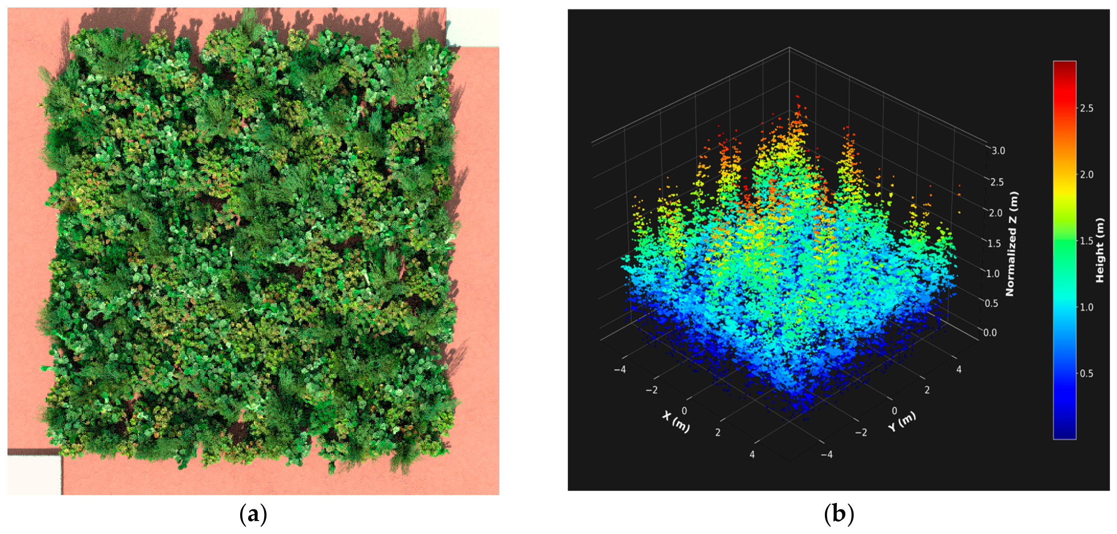
The integration of scene-building tools with comprehensive asset libraries has substantially enhanced our ability to simulate diverse and physically realistic fynbos ecosystems within the DIRSIG framework. Scenes can be instantiated to represent specific species compositions and fractional cover, thereby enabling the reconstruction of fynbos landscapes as a function of post-fire recovery stage. This capability allows controlled manipulation of ecological parameters while preserving biophysical realism. Figure 8 illustrates one example outcome of this workflow, presenting a representative scene corresponding to a 2006 burn within the fynbos ecosystem of the Grootbos Private Nature Reserve. The 2006 burn plot was selected as the representative site for quantitative validation because it had the most complete set of temporally matched reference data (UAS multispectral, AVIRIS-NG hyperspectral, and airborne LiDAR). The 2016 and 2019 plots were generated using the identical field parameterization and scene-generation workflow (Section 2 and Section 3) to demonstrate the framework’s applicability across different post-fire structural conditions but were not independently validated quantitatively in this study.
Figure 8a shows the generated 10 m × 10 m RGB scene produced using the proposed formulation, and Figure 8b presents the corresponding high-density simulated LiDAR point cloud. Together, these outputs demonstrate the framework’s ability to reproduce both spectral and structural attributes of post-fire shrubland environments. An additional strength of the framework is its scalability. We can rapidly instantiate larger scenes by modifying scene dimensions, enabling simulations across multiple spatial scales (e.g., 5 × 5 m or 100 × 100 m). This flexibility supports validation experiments and performance assessment of airborne imaging systems such as AVIRIS-NG, as well as UAS-based observations.
In subsequent subsections, we evaluate the simulated datasets against corresponding real-world observations. Because the synthetic scene is generated stochastically rather than reconstructed from the real landscape, the objective of this validation is not to achieve exact pixel- or point-level correspondence. Instead, the validation assesses whether the simulated data are consistent with the key spectral and structural characteristics of the observed ecosystem. Accordingly, quantitative comparisons were performed using sensor-specific, distribution-based metrics for the multispectral, hyperspectral, and LiDAR datasets to evaluate the suitability of the simulated scenes for methodological testing and performance analysis.

4.2. Simulated vs. Real UAS Multispectral Image (MSI)

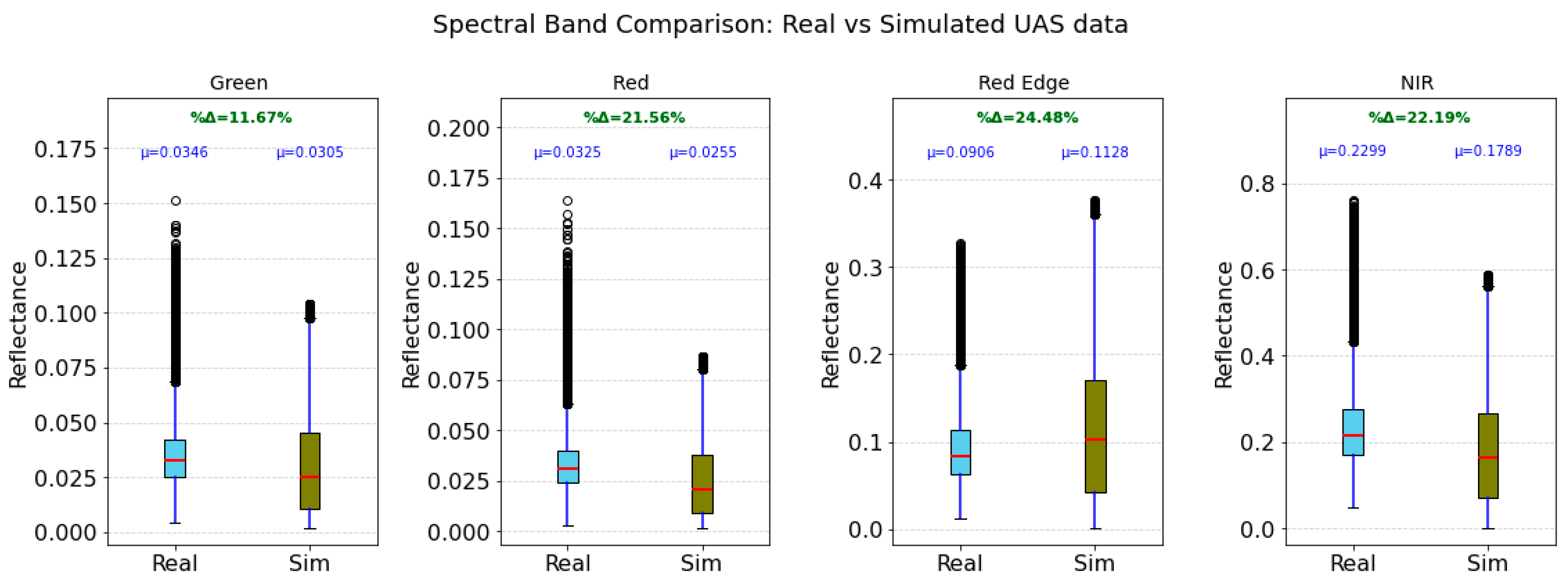
We simulated a four-band UAS multispectral image (MSI) in DIRSIG using the sensor specifications described in Table 2. The simulated bands correspond to the green, red, red-edge, and near-infrared (NIR) regions of the spectrum, consistent with the configuration of the field-acquired UAS MSI data. To evaluate the radiometric consistency between the simulated and real imagery, we compared band-wise reflectance distributions for the 2006 burn site. Figure 9 presents boxplots of the four spectral bands for both datasets, along with their corresponding mean values. The relative differences between simulated and real mean reflectance values were 11.67% (green), 21.56% (red), 24.48% (red-edge), and 22.19% (NIR). Overall, the discrepancy between simulated and observed reflectance ranged from 11.67 to 24.48%, with the smallest deviation occurring in the green band and the largest in the red-edge band. Although the simulated MSI data reproduced the general spectral behavior of the real UAS imagery, several factors likely contributed to these differences.
First, accurately replicating the heterogeneous background composition of fynbos ecosystems remains challenging. The real scene contains complex mixtures of deadwood, exposed soil, rocks, litter, and mixed soil–grass substrates. While representative background spectra were collected in the field, they cannot fully capture the fine-scale spatial and compositional variability present across the landscape. As a result, incomplete representation of sub-pixel background heterogeneity in the simulated scene likely contributed to reflectance differences.
Second, differences in radiometric calibration approaches introduce additional uncertainty. The UAS data acquired with the DJI platform were converted from radiance to reflectance using an upwelling–downwelling irradiance correction method [45]. In contrast, the simulated imagery was converted to reflectance using a two-point empirical line method (ELM) [46]. Variations in calibration methodology, reference targets, and illumination assumptions can produce systematic offsets between datasets.
Third, scene parameterization relied on field-based, visual estimates of species percentage cover and average canopy diameter measured by an expert botanist. Although ecologically informed, these measurements are inherently subjective and plot-based, and may not precisely represent the spatially continuous canopy structure captured by the UAS sensor. Differences between field-observed cover fractions and sensor-observed reflectance patterns may therefore also contribute to spectral mismatches.
Finally, atmospheric assumptions in the simulation represent another source of uncertainty. The simulated imagery was generated using a MODTRAN “50 km mid-latitude tropical” atmospheric model, with acquisition time approximated to solar noon. However, the exact environmental and meteorological conditions during UAS data collection—such as concentrations of CO2, CH4, tropospheric ozone, water vapor, and aerosol content—were not explicitly recreated. Variations in these parameters influence radiative transfer and reflectance retrieval, further contributing to discrepancies between simulated and real MSI data. Together, these factors explain the observed differences while supporting the overall validity of the simulation framework for representing post-fire fynbos spectral characteristics. We want to reinforce that our goal was not an exact match to real scene and sensor data, but rather a framework that mimics natural scene behavior and enables us to simulate physics-accurate sensing, while allowing us to vary scene and sensor parameters.
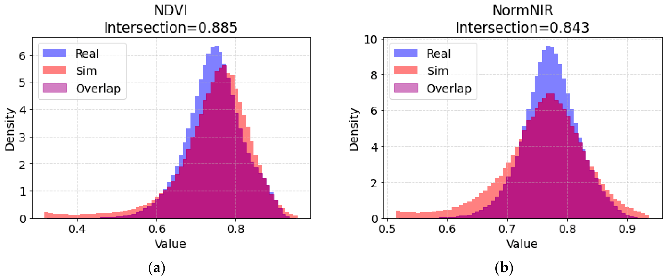
As an additional validation measure, we evaluated a suite of spectral vegetation indices from [47] to further assess the consistency between the real and simulated datasets. These indices were selected based on their demonstrated ability to correlate with key vegetation biophysical parameters. Table 4 presents a statistical comparison of vegetation indices derived from the real and simulated UAS multispectral imagery for the 2006 burn site. For each index, the mean and standard deviation quantify central tendency and variability, while the histogram intersection and Kolmogorov–Smirnov (K–S) statistic assess distributional similarity between datasets. Overall, the simulated indices reproduce the general magnitude and variability observed in the real data, although variability is consistently higher in the simulated imagery for several metrics (e.g., GNDVI, EVI, and SR). Histogram intersection values range from 0.683 to 0.886, indicating moderate to strong overlap between the distributions of real and simulated indices. Indices such as MSR, GDVI, IPVI, NDVI, RDVI, SR, TVI, and WDRVI (Wide Dynamic Range Vegetation Index) exhibit the highest distributional agreement (≥0.885), suggesting strong consistency in vegetation structure and vigor representation.
The K–S statistics further support this agreement, with relatively low values (0.075–0.363) across all indices, indicating limited divergence between cumulative distributions. Slightly higher K–S values for indices such as GSAVI and EVI suggest greater sensitivity to differences in canopy structure, soil background effects, or calibration inconsistencies between datasets. For a visual illustration, Figure 10 shows substantial overlap between the real and simulated distributions for NDVI and NormNIR, with high histogram intersection values (0.885 and 0.843, respectively). Collectively, these results demonstrate that the simulated MSI data effectively capture the spectral and biophysical patterns represented in the real UAS imagery, while highlighting specific indices that are more sensitive to scene parameterization and radiometric assumptions.

4.3. Simulated vs. Real Airborne Hyperspectral Data

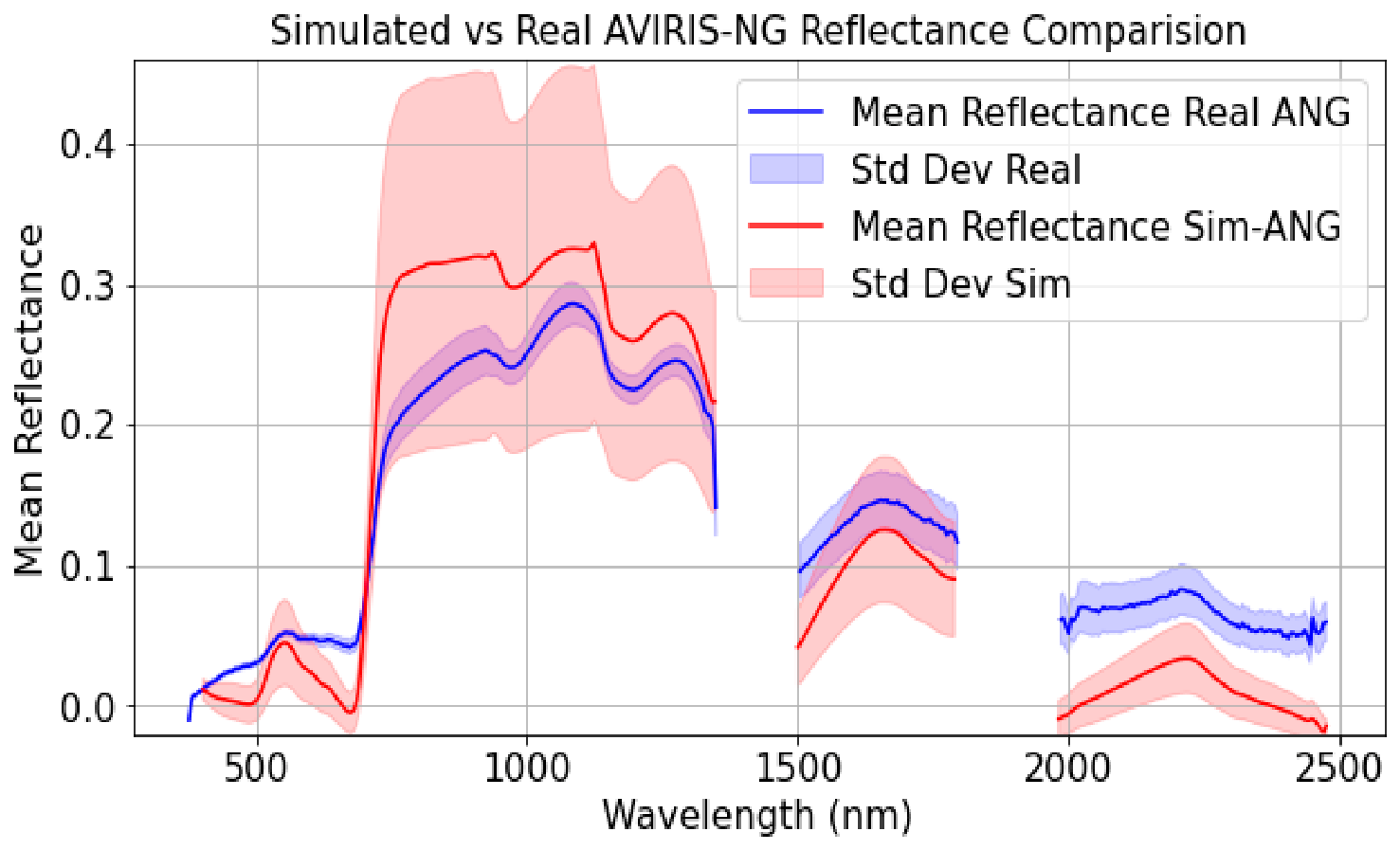
We next simulated an AVIRIS-NG hyperspectral image (HSI) over the fynbos study scene using instrument specifications provided by NASA JPL (Table 2), in order to evaluate the capability of DIRSIG in reproducing realistic imaging spectroscopy data. The simulation parameters were configured to match the AVIRIS-NG spectral characteristics, including wavelength range and band sampling, ensuring consistency with the 2024 NASA airborne campaign configuration. Detailed sensor-specific radiometric noise modeling was not explicitly implemented in this study. Figure 11 presents a comparison between the real AVIRIS-NG spectra and the simulated hyperspectral data. The results show that the simulated data successfully reproduce the overall spectral shape and key absorption features observed in the real measurements across the visible, near-infrared (NIR), and shortwave infrared (SWIR) regions (~400–2500 nm). The vegetation red-edge transition (~680–750 nm) and prominent leaf water absorption features (~970 and ~1200 nm) are well represented in the simulation. To complement the visual comparisons, we computed direct spectral similarity and error metrics between the real and simulated mean spectra after wavelength matching and exclusion of sensor-edge regions and strong atmospheric water-vapor absorption windows (~1340–1460 nm and ~1790–2100 nm) (Table 5). Across the full matched spectral range (~400–2450 nm), the simulated data achieved a Spectral Angle Mapper (SAM) of ~13.8°, RMSE of 0.045, normalized RMSE (NRMSE) of ~15.4%, and a Pearson correlation coefficient of r = 0.98, indicating strong overall agreement in spectral shape and magnitude. Region-specific comparisons showed consistently high agreement in the VNIR (400–1000 nm; SAM = 8.2°, r = 0.99) and SWIR1 (1000–1790 nm; SAM = 9.6°, r = 0.999), further supporting the close correspondence in red-edge- and NIR-driven spectral behavior described above. Agreement was substantially weaker in the SWIR2 region (2100–2450 nm), where SAM increased to 48.3° and NRMSE to 161%, despite a high correlation (r = 0.98). This discrepancy primarily reflects the systematic underestimation of reflectance in the simulated spectra, with mean reflectance of ~0.008 compared with ~0.063 in the real measurements. Because reflectance magnitudes in SWIR2 are inherently low, relatively small absolute differences can result in disproportionately large SAM and NRMSE values, even when the overall spectral shape remains highly correlated. The SWIR2 discrepancy is likely associated with atmospheric characterization. SWIR2 reflectance is particularly sensitive to atmospheric water-vapor effects, whereas the DIRSIG simulations used a generic MODTRAN built-in atmospheric profile rather than site- and date-specific atmospheric conditions corresponding to the AVIRIS-NG acquisition. We therefore attribute the observed SWIR2 underestimation primarily to potential differences between the assumed and actual atmospheric water-vapor and aerosol conditions. This interpretation is further supported by the absence of similarly pronounced discrepancies in the VNIR and SWIR1 regions, despite the use of the same sensor-noise treatment across the simulated spectrum. Thus, the SWIR2 discrepancy represents a limitation associated with the atmospheric assumptions used in the simulations rather than with the validation approach itself. Incorporating site- and date-specific atmospheric characterization is therefore an important priority for improving future DIRSIG scene simulations.
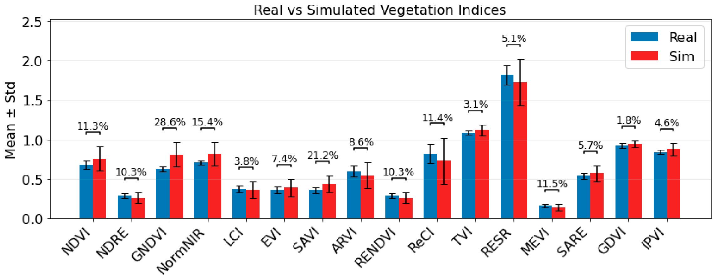
To further quantify spectral agreement, we compared a range of vegetation indices [47] derived from both datasets (Figure 12). Overall, the simulated indices exhibit comparable mean values to the real data, with percentage differences generally below ~15% for most metrics. Structural and red-edge-based indices, such as NDRE, RENDVI, LCI, and TVI, show relatively small deviations (3–10%), indicating good preservation of red-edge and chlorophyll-sensitive spectral behavior. Similarly, GDVI and IPVI demonstrate minimal differences (<5%), suggesting strong consistency in NIR-driven vegetation responses. Larger differences are observed for indices such as GNDVI (~28.6%) and SAVI (~21.3%), as well as NDVI (~11.4%) and NormNIR (~15.4%), where the simulated dataset tends to produce higher mean values and greater standard deviations. This increased variability, particularly evident in NIR-sensitive indices, is consistent with the broader spread observed in the spectral comparison (Figure 11). The larger standard deviations in the simulated indices likely reflect scene-level heterogeneity and modeling assumptions within DIRSIG.
Overall, the close agreement in spectral shape and the generally moderate percentage differences across a diverse set of vegetation indices demonstrate that DIRSIG effectively reproduces the dominant biophysical and spectral characteristics of AVIRIS-NG observations. The strong agreement in the VNIR and SWIR1 regions supports the suitability of the simulated imagery for subsequent controlled scene analyses, while the larger discrepancy in SWIR2 highlights a limitation associated primarily with the use of a generic atmospheric profile. Accordingly, SWIR2-dependent analyses should be interpreted with caution, and incorporating site- and date-specific atmospheric characterization would likely improve simulation fidelity in this region. Despite this limitation, the overall correspondence between the real and simulated datasets demonstrates the capability of DIRSIG to generate realistic hyperspectral imagery that approximates the spectral characteristics of the NASA 2024 airborne campaign.

4.4. Structural Metrics Comparison

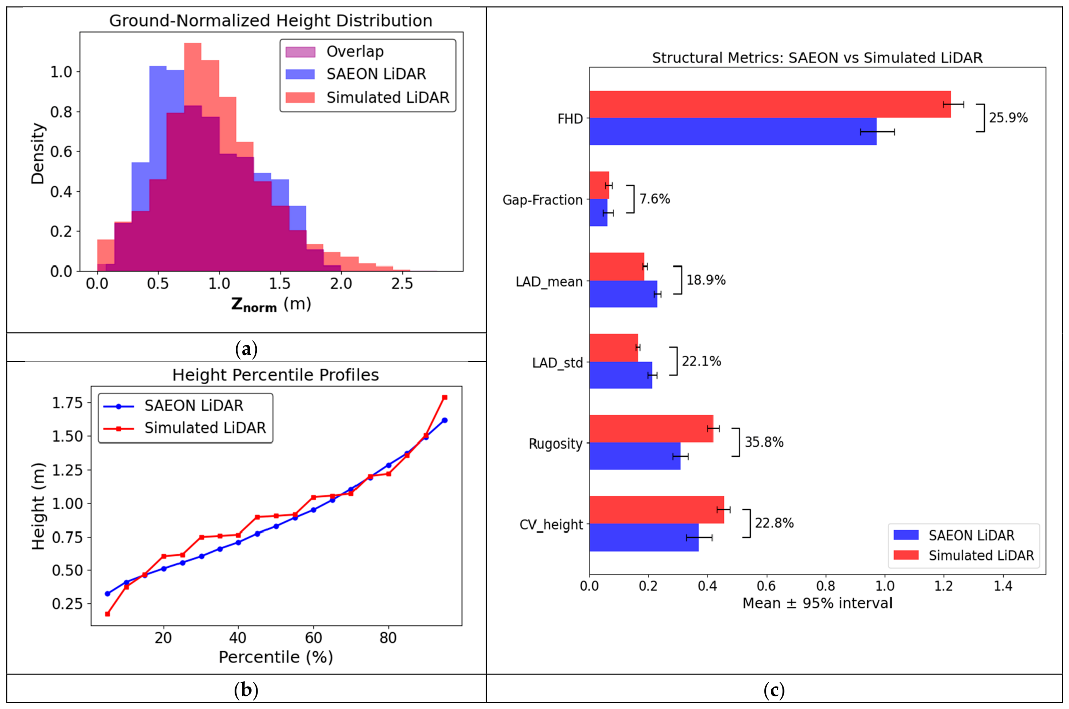
The individual 3D species models were developed using multiple sources of structural information, and hence we contend that they closely resemble vegetation structure observed in nature. While certain fine-scale attributes—such as crown overlap, leaf angle distributions, vertical layering, and leaf clustering—cannot be represented with complete fidelity, structural validation remains essential when these species models are assembled to reproduce shrubland communities. In this section, we compared a suite of structural metrics derived from simulated LiDAR data—generated using a discrete LiDAR system implemented in DIRSIG (see Table 3 for simulation parameters)—with corresponding metrics extracted from real SAEON Airborne Laser Scanning (ALS) [48] observations. This comparison ensures that, despite inherent differences in point density and acquisition geometry, both simulated and real point clouds capture comparable structural variability characteristic of fynbos shrublands.
The selected grain size was informed by a grid-size sensitivity analysis conducted from 1 to 5 m at 1 m intervals. We applied practical screening thresholds to identify the smallest grain that provided sufficient spatial coverage, point support, and metric stability. A grid cell was included only when it contained at least five LiDAR returns and at least 90% of all possible cells were required to meet this minimum. In addition, the median point count had to be at least 30 returns per cell to provide enough support for estimating the vertical structural metrics and the median change in metric values relative to the next larger grain had to be minimum. Although the 1 m grain provided 100 cells, it contained a median of only 13 returns per cell, and metric values changed by a median of 17.9% and a maximum of 51.3% between the 1 and 2 m grains. It therefore failed to meet the selection criteria. The 2 m grain was the smallest grain that met all criteria: all 25 expected cells contained at least five SAEON LiDAR returns and were included in the analysis, each cell contained at least 38 SAEON LiDAR returns, the median count of 52 returns per cell, and metric values changed by a median of 6.1% and a maximum of 10.6% between the 2 and 3 m grains. Importantly, this grid selection was based only on SAEON LiDAR sampling characteristics and metric stability, and not on agreement between the real and simulated datasets.
Prior to metric extraction, both point clouds were ground-normalized in CloudCompare (version 2.13.2; open-source, EDF R&D, Paris, France) to remove topographic effects. The SAEON ALS and simulated LiDAR point densities were 13.17 and 693.39 points/m2, respectively. To account for this difference, the simulated point cloud was randomly subsampled without replacement to match the total number of SAEON returns within the 10 m × 10 m area. In each repetition, each simulated return had an equal probability of being selected, and the procedure was independently repeated 100 times to account for variation introduced by random point selection. This procedure follows the repeated random-thinning approach previously used to evaluate the sensitivity of LiDAR structural metrics to point density [49]. For each repetition, each structural metric was averaged across the 25 grid cells. The median and the central 95% interval, defined by the 2.5th and 97.5th percentiles of the 100 repetition-level means, were reported for the simulated data. For the SAEON data, the mean and its 95% bootstrap confidence interval were estimated using 1000 resamples of the 25 grid-cell values with replacement. These uncertainty intervals are shown as error bars in the structural-metric comparison figure (Figure 13c).
The structural metrics were selected based on their proven capability to quantify three-dimensional vegetation structure, including vertical stratification, canopy cover, and surface roughness in shrublands and forests [50,51]. Specifically, we focused on metrics that are (i) widely used in ecological and LiDAR-based structural studies, (ii) interpretable in terms of physical canopy properties, and (iii) robust to differences in point density between ALS and simulated datasets. Accordingly, we computed foliage height diversity (FHD) [52], gap fraction (as proxy for LAI) [53], the mean and standard deviation of the leaf area distribution ( LAD mean , LAD std ) [54], rugosity, and the coefficient of variation in height ( CV height ) [50,55] for each grid cell in both datasets. At the selected 2 m × 2 m grain size, FHD exhibited clear systematic deviation between datasets, with mean values of approximately 0.0.97 for the SAEON ALS observations and 1.23 for the median density-matched simulated LiDAR. This higher FHD in the simulation suggests a more vertically stratified and evenly distributed canopy profile, potentially arising from the discrete and idealized placement of shrub species in the virtual scene, in contrast to the irregular and spatially heterogeneous structure of natural fynbos vegetation.
In comparison, gap fraction showed close agreement, with an SAEON mean of 0.0625 and a median density-matched simulated value of 0.0672, together with overlapping uncertainty intervals. The simulated LAD m e a n and LAD s t d   were lower than the real values by approximately 18.9% and 22.1%, respectively, whereas rugosity and CV h e i g h t were higher by approximately 35.8% and 22.8%. These differences indicate that the simulated canopy had greater overall height variability but a more even distribution of returns among the defined vertical layers. The direction of these differences remained consistent across the tested grain sizes, suggesting that they were not caused only by the selected 2 m grid. The height-percentile profiles and ground-normalized height distributions were calculated using all height returns within the full 10 m × 10 m area and were therefore independent of the selected grid size (see Figure 13a,b). These comparisons further support broad agreement in overall canopy height structure. The median height-percentile RMSE was 0.079 m. Similarly, the median histogram intersection between the two height distributions was 0.7680. This indicates that the overall difference between the two height distributions is very small. Simulated returns closely followed the SAEON percentile profile through most of the height distribution. Differences were most visible around the main distribution peak and in the upper tail, where the simulation modestly overestimated the tallest shrub heights. We therefore conclude that the DIRSIG-generated shrubland scene reproduces the dominant height distribution and general structural organization of mature fynbos vegetation. However, the remaining differences in fine-scale vertical complexity likely reflect idealized plant placement and structural simplifications inherent in the synthetic scene construction.

4.5. Limitations

Several factors bound the scope and precision of these results. Field parameterization—species composition, cover, and structural traits—reflects the specific communities sampled at Grootbos Private Nature Reserve; while the simulation framework itself is transferable to other fynbos sites given comparable field data, the conclusions presented here are specific to this reserve and should not be extrapolated to other fynbos landscapes or fire regimes without re-parameterization. The three plots sampled were burned in 2006, 2016, and 2019, spanning early-to-intermediate post-fire recovery; results do not extend to substantially younger or older successional stages outside the range. Within the simulated scenes, plant placement used a discrete, idealized instantiation procedure that does not capture fine-scale clustering, crown overlap, or growth-form variability observed in real stands (Section 4.4), and background heterogeneity—mixtures of deadwood, exposed soil, rocks, and litter—was represented using field-collected but spatially limited background spectra (Section 4.2). Species percent cover and canopy diameter were derived from expert, plot-based visual field estimates, which are inherently subjective and may not precisely match the spatially continuous cover captured by airborne sensors (Section 4.2). Topography was incorporated directly into the scene through UAS-derived terrain models, capturing local shading effects; illumination and atmospheric conditions, however, were fixed to a single representative setting (MODTRAN “50 km mid-latitude tropical” profile, solar noon) rather than matched to exact acquisition conditions or systematically varied (Section 4.2). This atmospheric simplification likely contributed to the lower spectral agreement observed in the SWIR2 region, where simulated reflectance was underestimated relative to the real AVIRIS-NG measurements. Radiometric calibration differences between the simulated (empirical line method) and real (irradiance-based) reflectance conversion introduce additional uncertainty in direct band-wise comparisons (Section 4.2).
Together, these factors bound the precision of pixel-level and point-level agreement between simulated and real data, and the generalizability of specific conclusions beyond the site and succession stages sampled. They do not, however, undermine the framework’s core objective of producing physically consistent, ecologically parameterized scenes for systematic experimentation.

5. Conclusions

This study presents a physics-based, three-dimensional simulation framework for reconstructing structurally complex and species-rich fynbos ecosystems within the DIRSIG environment. The framework allowed us to develop synthetic scenes that replicate both the spectral and structural characteristics of post-fire shrubland communities in the Greater Cape Floristic Region by integrating field-measured species composition, structural traits, and leaf-level optical properties with radiative transfer modeling and probabilistic spatial instantiation. Quantitative validation against real multispectral, hyperspectral, and LiDAR data was demonstrated for a representative 2006 post-fire plot. The same workflow was subsequently applied to construct scenes for the 2016 and 2019 post-fire plots, but the demonstrated quantitative validation remains limited to the representative 2006 plot.
Validation against real-world datasets—including UAS multispectral imagery, NASA AVIRIS-NG hyperspectral data, and airborne LiDAR—demonstrated good agreement in overall spectral shape, vegetation index behavior, and key structural metrics for the representative post-fire plot evaluated. While moderate deviations were observed in specific bands and spectral indices—particularly those sensitive to NIR variability, canopy stratification, and soil background effects—the simulated data reproduced the dominant biophysical and radiometric patterns of the real scene reasonably well. The larger discrepancy observed in the SWIR2 region represents a recognized limitation associated with the use of a generic atmospheric profile and highlights the importance of site- and date-specific atmospheric characterization in future simulations. Structural comparisons further confirmed that the simulated LiDAR point clouds captured foliage height diversity, canopy variability, and vertical distribution patterns characteristic of mature fynbos stands, with differences largely attributable to idealized plant placement and simplified canopy overlap in the virtual environment. These results are encouraging but remain dependent on the simplifying assumptions, single-site validation, and idealized representations discussed in Section 4.5, and should be interpreted as an initial demonstration of feasibility rather than a fully generalized validation.
Importantly, the objective of this framework is not exact pixel-level replication, but rather the creation of physically consistent, ecologically parameterized scenes suitable for controlled experimentation—that is, a virtual testbed in which sensor specifications and ecological parameters can each be varied systematically and independently, prior to any costly airborne or spaceborne data collection. By explicitly linking plant traits, species abundance, and structural configuration to sensor-specific radiometric outputs, the approach enables systematic exploration of how biodiversity signals propagate across spatial, spectral, and structural scales. This work establishes a scalable pathway for quantifying the theoretical and practical limits of species identification and biodiversity monitoring in fire-prone, heterogeneous ecosystems. The framework supports controlled sensitivity analyses of sensor specifications—such as spatial resolution, spectral sampling, and LiDAR point density—and provides a testbed for evaluating biodiversity metrics under known ecological conditions.
Ultimately, this simulation-based methodology provides a validated foundation to mechanistically investigate how spectral and structural leaf traits scale from individuals to landscapes and how these traits manifest as remotely sensed biodiversity proxies. Future work will use this capability to quantify information loss—for example, the drop in species spectral separability or classification accuracy as spatial or spectral resolution is degraded—and to identify the theoretical resolution thresholds at which species-level biodiversity signals can no longer be reliably detected. Such insights would be critical for informing future airborne and satellite mission design and for improving biodiversity monitoring strategies in globally significant ecosystems, such as the fynbos biome of the GCFR. Looking ahead, the framework is intended to provide a robust platform for hypothesis-driven scaling experiments directly relevant to current and forthcoming missions led by NASA. It supports informed mission planning, data interpretation, and long-term biodiversity monitoring in structurally heterogeneous landscapes by enabling controlled evaluation of sensor configurations and ecological complexity. For example, once a resolution threshold at which species-level signal collapses is identified for a given community, that threshold can directly inform minimum sensor specifications for future instrument design, guide flight-altitude and swath trade-offs for airborne campaigns, and help determine whether a given ecosystem’s biodiversity can be reliably tracked from spaceborne platforms or requires targeted airborne monitoring.

Author Contributions

Conceptualization, M.D.C. and J.v.A.; methodology, B.E. and M.D.C.; software, M.D.C. and B.E.; validation, M.D.C. and R.B.; formal analysis, M.D.C. and R.B.; investigation, M.D.C.; resources, J.v.A.; data curation, M.D.C. and B.E.; writing—original draft preparation, M.D.C.; writing—review and editing, J.v.A.; visualization, M.D.C. and R.B.; supervision, J.v.A.; project administration, J.v.A.; funding acquisition, J.v.A. All authors have read and agreed to the published version of the manuscript.

Funding

This research was funded by the NASA ROSES (Research Opportunities for Space and Earth Science) BioSCape program (NASA grant number #80NSSC22K0831).

Data Availability Statement

The datasets generated and analyzed for this study will be archived and made publicly available through the NASA BioSCape campaign’s data collection on the ORNL DAAC (Oak Ridge National Laboratory Distributed Active Archive Center), in accordance with NASA’s open data policy.

Acknowledgments

We are grateful to Ross Turner and Sean Privett of the Grootbos Private Nature Reserve in South Africa for providing invaluable botanical and field expertise. The authors also thank the South African Environmental Observation Network (NRF-SAEON) for data access. LiDAR data were sourced from the Airborne Remote Sensing Platform of the Shallow Marine and Coastal Research Infrastructure (SMCRI), managed by the NRF-SAEON Elwandle Coastal Node of the National Research Foundation of South Africa.

Conflicts of Interest

The authors declare no conflicts of interest.

References

  1. Snijman, D. Plants of the Greater Cape Floristic Region. 2: The Extra Cape Flora; SANBI: Cape Town, South Africa, 2013. [Google Scholar]
  2. Myers, N.; Mittermeier, R.A.; Mittermeier, C.G.; Da Fonseca, G.A.; Kent, J. Biodiversity hotspots for conservation priorities. Nature 2000, 403, 853–858. [Google Scholar] [CrossRef] [Scilit] [PubMed]
  3. Moncrieff, G.R. Locating and dating land cover change events in the Renosterveld, a Critically Endangered shrubland ecosystem. Remote Sens. 2021, 13, 834. [Google Scholar] [CrossRef] [Scilit]
  4. Slingsby, J.A.; Moncrieff, G.R.; Rogers, A.J.; February, E.C. Altered ignition catchments threaten a hyperdiverse fire-dependent ecosystem. Glob. Change Biol. 2020, 26, 616–628. [Google Scholar] [CrossRef] [Scilit] [PubMed]
  5. Slingsby, J.A.; Merow, C.; Aiello-Lammens, M.; Allsopp, N.; Hall, S.; Kilroy Mollmann, H.; Turner, R.; Wilson, A.M.; Silander, J.A. Intensifying postfire weather and biological invasion drive species loss in a Mediterranean-type biodiversity hotspot. Proc. Natl. Acad. Sci. USA 2017, 114, 4697–4702. [Google Scholar] [CrossRef] [Scilit] [PubMed]
  6. Cardoso, A.W.; Hestir, E.L.; Slingsby, J.A.; Forbes, C.J.; Moncrieff, G.R.; Turner, W.; Skowno, A.L.; Nesslage, J.; Brodrick, P.G.; Gaddis, K.D.; et al. The biodiversity survey of the Cape (BioSCape), integrating remote sensing with biodiversity science. npj Biodivers. 2025, 4, 2. [Google Scholar] [CrossRef] [Scilit] [PubMed]
  7. Brown, N. Promotion of germination of fynbos seeds by plant-derived smoke. New Phytol. 1993, 123, 575–583. [Google Scholar] [CrossRef] [Scilit] [PubMed]
  8. Allsopp, N.; Colville, J.F.; Verboom, G.A. Fynbos: Ecology, Evolution, and Conservation of a Megadiverse Region; Oxford University Press: Oxford, UK, 2014. [Google Scholar]
  9. Verboom, G.A.; Slingsby, J.A.; Cramer, M.D. Fire-modulated fluctuations in nutrient availability stimulate biome-scale floristic turnover in time, and elevated species richness, in low-nutrient fynbos heathland. Ann. Bot. 2024, 133, 819–832. [Google Scholar] [CrossRef] [Scilit] [PubMed]
  10. Mi, X.; Feng, G.; Hu, Y.; Zhang, J.; Chen, L.; Corlett, R.T.; Hughes, A.C.; Pimm, S.; Schmid, B.; Shi, S. The global significance of biodiversity science in China: An overview. Natl. Sci. Rev. 2021, 8, nwab032. [Google Scholar] [CrossRef] [Scilit] [PubMed]
  11. Asner, G.P.; Martin, R.E. Spectranomics: Emerging science and conservation opportunities at the interface of biodiversity and remote sensing. Glob. Ecol. Conserv. 2016, 8, 212–219. [Google Scholar] [CrossRef] [Scilit]
  12. Dahlin, K.M. Spectral diversity area relationships for assessing biodiversity in a wildland–agriculture matrix. Ecol. Appl. 2016, 26, 2758–2768. [Google Scholar] [CrossRef] [Scilit] [PubMed]
  13. Gholizadeh, H.; Gamon, J.A.; Townsend, P.A.; Zygielbaum, A.I.; Helzer, C.J.; Hmimina, G.Y.; Yu, R.; Moore, R.M.; Schweiger, A.K.; Cavender-Bares, J. Detecting prairie biodiversity with airborne remote sensing. Remote Sens. Environ. 2019, 221, 38–49. [Google Scholar] [CrossRef] [Scilit]
  14. Yip, K.H.A.; Liu, R.; Wu, J.; Hau, B.C.H.; Lin, Y.; Zhang, H. Community-based plant diversity monitoring of a dense-canopy and species-rich tropical forest using airborne LiDAR data. Ecol. Indic. 2024, 158, 111346. [Google Scholar] [CrossRef] [Scilit]
  15. Zheng, Z.; Zeng, Y.; Schneider, F.D.; Zhao, Y.; Zhao, D.; Schmid, B.; Schaepman, M.E.; Morsdorf, F. Mapping functional diversity using individual tree-based morphological and physiological traits in a subtropical forest. Remote Sens. Environ. 2021, 252, 112170. [Google Scholar] [CrossRef] [Scilit]
  16. Bhatta, R.; Chaity, M.D.; Chancia, R.O.; Slingsby, J.; Moncrieff, G.; van Aardt, J. Assessment of Structural Differences in a Low-Stature Mediterranean-Type Shrubland Using Structure-From-Motion (SfM). Remote Sens. 2025, 17, 2784. [Google Scholar] [CrossRef] [Scilit]
  17. eResearch, University of Cape Town. Mapping Pixels: Bridging the Gap Between Individual Plants and Satellite Imagery. Available online: https://www.uct.ac.za/eresearch/articles/2018-02-26-mapping-pixels (accessed on 29 May 2026).
  18. Paz-Kagan, T.; Chang, J.G.; Shoshany, M.; Sternberg, M.; Karnieli, A. Assessment of plant species distribution and diversity along a climatic gradient from Mediterranean woodlands to semi-arid shrublands. GISci. Remote Sens. 2021, 58, 929–953. [Google Scholar] [CrossRef] [Scilit]
  19. Masemola, C.; Cho, M.A.; Ramoelo, A. Towards a semi-automated mapping of Australia native invasive alien Acacia trees using Sentinel-2 and radiative transfer models in South Africa. ISPRS J. Photogramm. Remote Sens. 2020, 166, 153–168. [Google Scholar] [CrossRef] [Scilit]
  20. Qi, J.; Xie, D.; Yin, T.; Yan, G.; Gastellu-Etchegorry, J.-P.; Li, L.; Zhang, W.; Mu, X.; Norford, L.K. LESS: LargE-Scale remote sensing data and image simulation framework over heterogeneous 3D scenes. Remote Sens. Environ. 2019, 221, 695–706. [Google Scholar] [CrossRef] [Scilit]
  21. Schott, J.R.; Brown, S.D.; Raqueno, R.V.; Gross, H.N.; Robinson, G. An advanced synthetic image generation model and its application to multi/hyperspectral algorithm development. Can. J. Remote Sens. 1999, 25, 99–111. [Google Scholar] [CrossRef] [Scilit]
  22. Schott, J.R.; Raqueno, R.V.; Salvaggio, C. Incorporation of a time-dependent thermodynamic model and a radiation propagation model into IR 3D synthetic image generation. Opt. Eng. 1992, 31, 1505–1516. [Google Scholar] [CrossRef] [Scilit]
  23. Brown, S.D.; Blevins, D.D.; Schott, J.R. Time-gated topographic LIDAR scene simulation. In Proceedings of Laser Radar Technology and Applications X; SPIE: Bellingham, WA, USA, 2005; pp. 342–353. [Google Scholar]
  24. Burton, R.R.; Schott, J.R.; Brown, S.D. Elastic LADAR modeling for synthetic imaging applications. In Proceedings of Imaging Spectrometry VIII; SPIE: Bellingham, WA, USA, 2002; pp. 144–155. [Google Scholar]
  25. Flusche, B.M.; Gartley, M.G.; Schott, J.R. Exploiting spectral and polarimetric data fusion to enhance target detection performance. In Proceedings of Imaging Spectrometry XV; SPIE: Bellingham, WA, USA, 2010; pp. 79–88. [Google Scholar]
  26. Ientilucci, E.J.; Brown, S.D.; Schott, J.R.; Raqueno, R.V. Multispectral Simulation Environment for Modeling Low-Light-Level Sensor Systems; SPIE: Bellingham, WA, USA, 1998; pp. 10–19. [Google Scholar]
  27. Gartley, M.; Goodenough, A.; Brown, S.; Kauffman, R.P. A comparison of spatial sampling techniques enabling first principles modeling of a synthetic aperture RADAR imaging platform. In Proceedings of Algorithms for Synthetic Aperture Radar Imagery XVII; SPIE: Bellingham, WA, USA, 2010; pp. 220–229. [Google Scholar]
  28. Chaity, M.D.; van Aardt, J. Exploring the Limits of Species Identification via a Convolutional Neural Network in a Complex Forest Scene through Simulated Imaging Spectroscopy. Remote Sens. 2024, 16, 498. [Google Scholar] [CrossRef] [Scilit]
  29. Yao, W.; van Aardt, J.; van Leeuwen, M.; Kelbe, D.; Romanczyk, P. A simulation-based approach to assess subpixel vegetation structural variation impacts on global imaging spectroscopy. IEEE Trans. Geosci. Remote Sens. 2018, 56, 4149–4164. [Google Scholar] [CrossRef]
  30. Yao, W.; Kelbe, D.; Leeuwen, M.v.; Romanczyk, P.; Aardt, J.v. Towards an improved LAI collection protocol via simulated and field-based PAR sensing. Sensors 2016, 16, 1092. [Google Scholar] [CrossRef] [Scilit] [PubMed]
  31. Romanczyk, P.; van Aardt, J.; Cawse-Nicholson, K.; Kelbe, D.; McGlinchy, J.; Krause, K. Assessing the impact of broadleaf tree structure on airborne full-waveform small-footprint LiDAR signals through simulation. Can. J. Remote Sens. 2013, 39, S60–S72. [Google Scholar] [CrossRef] [Scilit]
  32. Wu, J.; Van Aardt, J.; Asner, G.P. A comparison of signal deconvolution algorithms based on small-footprint LiDAR waveform simulation. IEEE Trans. Geosci. Remote Sens. 2011, 49, 2402–2414. [Google Scholar] [CrossRef] [Scilit]
  33. Wu, J.; Van Aardt, J.; McGlinchy, J.; Asner, G.P. A robust signal preprocessing chain for small-footprint waveform lidar. IEEE Trans. Geosci. Remote Sens. 2012, 50, 3242–3255. [Google Scholar] [CrossRef] [Scilit]
  34. Wu, J.; Cawse-Nicholson, K.; van Aardt, J. 3D Tree reconstruction from simulated small footprint waveform lidar. Photogramm. Eng. Remote Sens. 2013, 79, 1147–1157. [Google Scholar] [CrossRef] [Scilit]
  35. Bhatta, R.; Chaity, M.D.; Aardt, J.V. A Novel Data-Driven Approach to Leaf Area Index Modeling Using High-Fidelity Simulation-Based Full-Waveform LiDAR Data. IEEE J. Sel. Top. Appl. Earth Obs. Remote Sens. 2026, 19, 4693–4716. [Google Scholar] [CrossRef] [Scilit]
  36. Aardt, J.V.; Arthur, M.; Sovkoplas, G.; Swetnam, T.L. LiDAR-Based Estimation of Forest Floor Fuel Loads Using a Novel Distributional Approach; IEEE: Piscataway, NJ, USA, 2011. [Google Scholar]
  37. Wu, J.; Van Aardt, J.; Asner, G.; Mathieu, R.; Kennedy-Bowdoin, T.; Knapp, D.; Wessels, K.; Erasmus, B.; Smit, I. Connecting the dots between laser waveforms and herbaceous biomass for assessment of land degradation using small-footprint waveform lidar data. In Proceedings of 2009 IEEE International Geoscience and Remote Sensing Symposium; IEEE: Piscataway, NJ, USA, 2009; pp. II-334–II-337. [Google Scholar]
  38. Mlambo, R.; Woodhouse, I.H.; Gerard, F.; Anderson, K. Structure from motion (SfM) photogrammetry with drone data: A low cost method for monitoring greenhouse gas emissions from forests in developing countries. Forests 2017, 8, 68. [Google Scholar] [CrossRef] [Scilit]
  39. Iglhaut, J.; Cabo, C.; Puliti, S.; Piermattei, L.; O’Connor, J.; Rosette, J. Structure from motion photogrammetry in forestry: A review. Curr. For. Rep. 2019, 5, 155–168. [Google Scholar] [CrossRef] [Scilit]
  40. Privett, S.; Lutzeyer, H. Field guide to the flora of Grootbos Nature Reserve and the Walker Bay Region; Grootbos Foundation: Gansbaai, South Africa, 2010. [Google Scholar]
  41. Jacquemoud, S.; Baret, F. PROSPECT: A model of leaf optical properties spectra. Remote Sens. Environ. 1990, 34, 75–91. [Google Scholar] [CrossRef] [Scilit]
  42. Bridson, R. Fast Poisson disk sampling in arbitrary dimensions. SIGGRAPH Sketches 2007, 10, 1. [Google Scholar]
  43. Cook, R.L. Stochastic sampling in computer graphics. ACM Trans. Graph. 1986, 5, 51–72. [Google Scholar] [CrossRef] [Scilit]
  44. Berk, A.; Anderson, G.; Bernstein, L.; Acharya, P.; Dothe, H.; Matthew, M.; Adler-Golden, S.; Chetwynd, J.; Richtsmeier, S.; Pukall, B.; et al. MODTRAN4 Radiative Transfer Modeling for Atmospheric Correction; SPIE: Bellingham, WA, USA, 1999; Volume 3756. [Google Scholar]
  45. Köppl, C.J.; Malureanu, R.; Dam-Hansen, C.; Wang, S.; Jin, H.; Barchiesi, S.; Serrano Sandí, J.M.; Muñoz-Carpena, R.; Johnson, M.; Durán-Quesada, A.M.; et al. Hyperspectral reflectance measurements from UAS under intermittent clouds: Correcting irradiance measurements for sensor tilt. Remote Sens. Environ. 2021, 267, 112719. [Google Scholar] [CrossRef] [Scilit]
  46. Conel, J.E.; Green, R.O.; Vane, G.; Bruegge, C.J.; Alley, R.E.; Curtiss, B.J. AIS-2 radiometry and a comparison of methods for the recovery of ground reflectance. In Proceedings of the 3rd Airborne Imaging Spectrometer Data Analysis Workshop.Pasadena, CA, USA, 2–4 June 1987; Vane, G., Ed.; JPL Publication 87-30; Jet Propulsion Laboratory: Pasadena, CA, USA, 1987; pp. 18–47. [Google Scholar]
  47. Chaity, M.D.; Chancia, R.; Bhatta, R.; Slingsby, J.; Moncrieff, G.; van Aardt, J. Advancing Mediterranean biodiversity monitoring in South Africa through machine learning and cost-effective UAS imagery. J. Geophys. Res. Biogeosci. 2026, 131, e2025JG009096. [Google Scholar] [CrossRef] [Scilit]
  48. Shallow Marine and Coastal Research Infrastructure (SMCRI). Aligned Point Cloud Files for Grootbos Nature Reserve, South Africa; South African Environmental Observation Network (NRF-SAEON), Elwandle Coastal Node: Gqeberha, South Africa, 2026. [Google Scholar] [CrossRef]
  49. LaRue, E.A.; Fahey, R.; Fuson, T.L.; Foster, J.R.; Matthes, J.H.; Krause, K.; Hardiman, B.S. Evaluating the sensitivity of forest structural diversity characterization to LiDAR point density. Ecosphere 2022, 13, e4209. [Google Scholar] [CrossRef] [Scilit]
  50. Atkins, J.W.; Costanza, J.; Dahlin, K.M.; Dannenberg, M.P.; Elmore, A.J.; Fitzpatrick, M.C.; Hakkenberg, C.R.; Hardiman, B.S.; Kamoske, A.; LaRue, E.A. Scale dependency of lidar-derived forest structural diversity. Methods Ecol. Evol. 2023, 14, 708–723. [Google Scholar] [CrossRef] [Scilit]
  51. Ehbrecht, M.; Schall, P.; Juchheim, J.; Ammer, C.; Seidel, D. Effective number of layers: A new measure for quantifying three-dimensional stand structure based on sampling with terrestrial LiDAR. For. Ecol. Manag. 2016, 380, 212–223. [Google Scholar] [CrossRef] [Scilit]
  52. Tang, H.; Armston, J.; Dubayah, R. Algorithm Theoretical Basis Document (ATBD) for GEDI L2B Footprint Canopy Cover and Vertical Profile Metrics; Goddard Space Flight Center: Greenbelt, MD, USA, 2019.
  53. Morsdorf, F.; Kötz, B.; Meier, E.; Itten, K.; Allgöwer, B. Estimation of LAI and fractional cover from small footprint airborne laser scanning data based on gap fraction. Remote Sens. Environ. 2006, 104, 50–61. [Google Scholar] [CrossRef] [Scilit]
  54. Almeida, D.R.A.; Stark, S.C.; Shao, G.; Schietti, J.; Nelson, B.W.; Silva, C.A.; Gorgens, E.B.; Valbuena, R.; Papa, D.d.A.; Brancalion, P.H.S. Optimizing the Remote Detection of Tropical Rainforest Structure with Airborne Lidar: Leaf Area Profile Sensitivity to Pulse Density and Spatial Sampling. Remote Sens. 2019, 11, 92. [Google Scholar] [CrossRef] [Scilit]
  55. Kane, V.R.; McGaughey, R.J.; Bakker, J.D.; Gersonde, R.F.; Lutz, J.A.; Franklin, J.F. Comparisons between field-and LiDAR-based measures of stand structural complexity. Can. J. For. Res. 2010, 40, 761–773. [Google Scholar] [CrossRef] [Scilit]
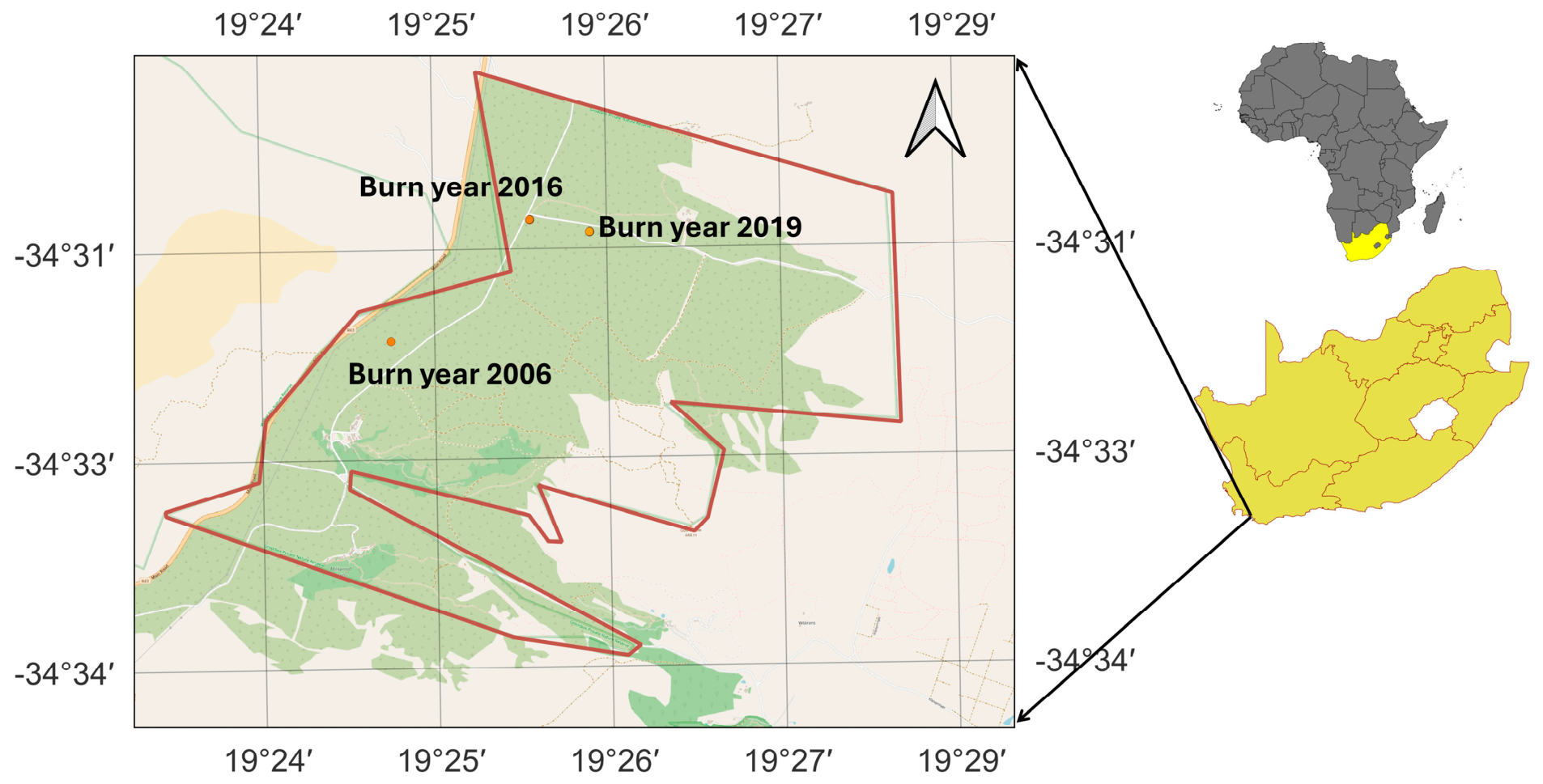
Figure 1. Study area in Grootbos Private Nature Reserve in South Africa. The three chosen plots are depicted in circles, and the associated year represents when the plot was last burned.
Remotesensing 18 02816 g001
Figure 2. An example array of (a) leaf spectral data of Erica irregularis plant and (b) background soil spectra from the 2006 burn plot was collected by the team using an Analytical Spectral Device (ASD) field spectroradiometer in the of 350–2500 nm spectral range.
Remotesensing 18 02816 g002
Figure 3. (a) Point cloud representation of the raw data collected by the drone flight over fynbos 2019 burn plot in CloudCompare (version 2.13.2; open-source, EDF R&D, Paris, France); (b) point clouds are facetized into a usable 3D mesh in CloudCompare; and (c) retopologized and processed 3D mesh for accurate ground measurements in MAYA 2024. The resulting terrain model represents a 66 m × 66 m area of the study site.
Remotesensing 18 02816 g003
Figure 4. These example 3D models were created by taking real-world examples of each species for reference and recreating each one with as much accuracy as possible by mirroring the structure of plants from the leaves to the stems. Some larger assets, like larger shrubs, are generated via node structures, which create armature and leaf attribution. The DIRSIG simulation team used Maya and Blender to create these 3D models.
Remotesensing 18 02816 g004
Figure 5. Reflectance and transmittance spectra of Metalsia muricata species; the transmittance curve was produced using PROSPECT (pypi.org/project/prosail).
Remotesensing 18 02816 g005
Figure 6. Workflow for spatially distributing species instances using blue noise sampling constrained by a probability map derived from multispectral UAS imagery.
Remotesensing 18 02816 g006
Figure 7. This density map is created by selecting a random subset (in red) of the drone image (left) of the desired burn plot run through a classification algorithm (right).
Remotesensing 18 02816 g007
Figure 8. Example of plot-to-landscape level simulated scenes of fynbos that were burned in 2006 in Grootbos Private Nature Reserve. The scenes are dimensions of (10 × 10 m) captured using (a) a DJI MAVIC 3 multispectral camera at 50 m altitude with 2.5 cm GSD and (b) high-density simulated LiDAR point cloud corresponding to the modeled scene.
Remotesensing 18 02816 g008
Figure 9. Boxplot comparison of real and simulated UAS multispectral reflectance for the 2006 burn site across four spectral bands (green, red, red-edge, and NIR). Mean reflectance values (µ) are shown above each distribution, along with the percentage difference (%Δ) between simulated and real data.
Remotesensing 18 02816 g009
Figure 10. Histogram of (a) NDVI and (b) Normalized NIR (NormNIR) derived from real and simulated UAS multispectral imagery for the 2006 burn site. Histogram overlap is quantified using the intersection metric, with values of 0.885 for NDVI and 0.843 for NormNIR, indicating strong distributional agreement between datasets.
Remotesensing 18 02816 g010
Figure 11. Comparison of mean reflectance spectra and associated variability for real (blue) and simulated (red) AVIRIS-NG (ANG) data across the full wavelength range. Shaded areas represent ±1 standard deviation.
Remotesensing 18 02816 g011
Figure 12. Comparison of mean and standard deviation of selected vegetation indices derived from real and simulated AVIRIS-NG datasets. Bars represent the average index values across the region of interest, with error bars indicating one standard deviation. Percentage values above each pair denote the relative percentage difference between simulated and real means, highlighting overall agreement in central tendency and variability between real and simulated values across all indices. Abbreviation: NDVI—Normalized Difference Vegetation Index, NDRE—Normalized Difference Red-Edge Index, GNDVI—Green Normalized Difference Vegetation Index, NormNIR—Normalized Near-Infrared Reflectance, LCI—Leaf Chlorophyll Index, EVI—Enhanced Vegetation Index, SAVI—Soil-Adjusted Vegetation Index, ARVI—Atmospherically Resistant Vegetation Index, RENDVI—Red-Edge Normalized Difference Vegetation Index, ReCI—Red-Edge Chlorophyll Index, TVI—Transformed Vegetation Index, RESR—Red-Edge Simple Ratio, MEVI—Modified Enhanced Vegetation Index, SARE—Soil-Adjusted Red-Edge Index, GDVI—Green Difference Vegetation Index, IPVI—Infrared Percentage Vegetation Index.
Remotesensing 18 02816 g012
Figure 13. Validation results comparing structural metrics between SAEON real LiDAR and simulated DIRSIG LiDAR data: (a) ground normalized height distribution; (b) height percentile profiles; and (c) comparison of structural metrics, showing close structural resemblance between the dataset. Grid-based LiDAR structural metrics were extracted from both datasets using a validation grain of 2 m × 2 m, resulting in 25 grid cells per scene. The selected grid size was informed by a grid-size versus metric-sensitivity analysis, which indicated that ~2 m provides a stable balance between resolving shrub-scale structural heterogeneity and minimizing sampling artifacts present at finer resolutions.
Remotesensing 18 02816 g013
Table 1. Summary of plot-level vegetation data for the 2006 burn year.
TaxonMean Diameter
(cm)
Percentage Cover (%)Height
(max, m)
Metalasia muricata15121.78
Passerina corymbosa35151.33
Erica irregularis40200.67
Chironia baccifera150.50.5
Indigofera brachystachya40150.67
Euclea racemosa3552.67
Anthospermum aethiopicum2560.89
Restio eleocharis5050.5
Cassytha ciliolata502.50.5
Pterocelastrus tricuspidatus10052.22
Hermannia ternifolia2520.5
Clutia alaternoides2020.5
Deadwood10100.89
Table 2. Summary of the imaging spectrometer data used in this paper.
Hyperspectral ImagerAVIRIS NGDJI MAVIC 3 MSI
Spectral Bands4254
Spectral Range380–2500-
Spectral Sampling5 nm± 0.5 nmGreen: 560 ± 16 nm
Red: 650 ± 16 nm
Red-Edge: 730 ± 16 nm
NIR: 860 ± 26 nm
Pixel Array640 × 480640 × 480
Pixel Size27 microns2 microns
Focal Length26.60 mm4 mm
Flying Height1 km50 m
GSD (Ground Sampling Distance)3 m2.5 cm
Table 3. Summary of a low pulse-width multi-pulse discrete LiDAR system.
Collection ParametersValues
Platform height 50 m
Beam shapeGaussian
Half beam divergence 0.071 rad
Circular footprint diameter
Ground coverage per run
Number of runs needed to cover the scene
~7.11 m
5 m × 5 m
4 (adjacent frame positions)
Array dimension128 × 128 (each 100 microns)
Wavelength1064 nm (Gaussian: Line width = 0.01 nm)
Focal length12.8 cm
GSD0.04 m
Pulse width2 ns (Gaussian)
PRF (pulse repetition frequency)1 Hz
Range limits (min, max) 40–50 m @15 cm samples
Table 4. Statistical comparison of vegetation indices derived from real and simulated UAS multispectral imagery for the 2006 burn site. For each metric, the mean ± standard deviation (std) are reported for both datasets. Distributional similarity between real and simulated indices is quantified using histogram intersection and the Kolmogorov–Smirnov (K–S) test statistic. Higher histogram intersection values indicate greater overlap between distributions, while lower K–S statistics indicate stronger agreement.
MetricReal
(Mean ± Std)
Simulated
(Mean ± Std)
Histogram
Intersection
Kolmogorov–Smirnov (K-S) Test
ARI24.2901 ± 1.35674.9318 ± 3.85910.7860.137
EVI0.4192 ± 0.14160.3331 ± 0.21900.7550.334
GCI5.9247 ± 1.60215.5156 ± 3.97440.7280.252
GDVI0.9538 ± 0.04710.9183 ± 0.18940.8860.075
GNDVI0.7379 ± 0.04990.6819 ± 0.16230.7280.252
GRNDVI0.5451 ± 0.09160.4936 ± 0.20660.8430.147
GSAVI0.3736 ± 0.08650.2822 ± 0.16000.7500.363
IPVI0.8731 ± 0.08760.8599 ± 0.08280.8850.075
MSR2.1956 ± 0.55802.1608 ± 0.78410.8850.075
NDVI0.7462 ± 0.07380.7198 ± 0.16560.8850.075
NDWI−0.7379 ± 0.0499−0.6819 ± 0.16230.7280.252
NormG0.1158 ± 0.01880.1363 ± 0.05190.6830.288
NormNIR0.7726 ± 0.08940.7468 ± 0.10330.8430.147
NormR0.1117 ± 0.02880.1169 ± 0.05240.8710.077
OSAVI0.4534 ± 0.08110.3634 ± 0.16450.8070.322
RDVI0.8628 ± 0.09220.8531 ± 0.07880.8850.075
RVI6.9247 ± 1.64756.5156 ± 3.97440.7280.252
SR7.6327 ± 2.98927.7233 ± 4.04240.8860.075
TVI1.1159 ± 0.08901.1006 ± 0.09230.8850.075
WDRVI−0.4623 ± 0.1356−0.4674 ± 0.17840.8850.075
Abbreviation: ARI2—Anthocyanin Reflectance Index 2, EVI—Enhanced Vegetation Index, GCI—Green Chlorophyll Index, GDVI—Green Difference Vegetation Index, GNDVI—Green Normalized Difference Vegetation Index, GRNDVI—Green-Red Normalized Difference Vegetation Index, GSAVI—Green Soil-Adjusted Vegetation Index, IPVI—Infrared Percentage Vegetation Index, MSR—Modified Simple Ratio, NDVI—Normalized Difference Vegetation Index, NDWI—Normalized Difference Water Index, NormG—Normalized Green Reflectance, NormNIR—Normalized Near-Infrared Reflectance, NormR—Normalized Red Reflectance, OSAVI—Optimized Soil-Adjusted Vegetation Index, RDVI—Renormalized Difference Vegetation Index, RVI—Ratio Vegetation Index, SR-Simple Ratio, TVI—Transformed Vegetation Index, WDRVI—Wide Dynamic Range Vegetation Index.
Table 5. Quantitative spectral similarity and error metrics between real and simulated AVIRIS-NG (ANG) mean reflectance spectra, computed on wavelength-matched bands after excluding sensor edges and atmospheric water-vapor absorption windows (~1340–1460 nm and ~1790–2100 nm). Metrics are reported for the full matched spectrum (~400–2450 nm) and separately for the VNIR (400–1000 nm), SWIR1 (1000–1790 nm), and SWIR2 (2100–2450 nm) spectral regions. SAM = Spectral Angle Mapper (degrees); RMSE = root-mean-square error; NRMSE = normalized RMSE (%, normalized by the range of the real spectrum); r = Pearson correlation coefficient.
ScopeSAM (°)RMSENRMSE (%)Pearson (r)
Full spectrum13.770.044515.430.9761
VNIR 400–1000 nm8.150.047518.820.9903
SWIR1 1000–1790 nm9.550.034515.770.9987
SWIR2 2100–2450 nm48.310.0548161.220.9818
Disclaimer/Publisher’s Note: The statements, opinions and data contained in all publications are solely those of the individual author(s) and contributor(s) and not of MDPI and/or the editor(s). MDPI and/or the editor(s) disclaim responsibility for any injury to people or property resulting from any ideas, methods, instructions or products referred to in the content.