Multiple Vegetation Indicators Reveal Contrasting Post-Drought Recovery Time in the Yangtze River Basin Following the 2022 Extreme Drought

Highlights

What are the main findings?

• This study analyzes vegetation recovery after the extreme drought event across the Yangtze River Basin in 2022.
• Vegetation recovery timing exhibits distinct differences among multiple remote-sensing indicators.
• Recovery timing varies substantially across different vegetation types.
• LAI shows the shortest recovery time, whereas GPP presents the longest recovery period.
• Forest and grassland achieve faster recovery, while cropland and shrubland exhibit relatively slow recovery.

What are the implications of the main findings?

• Multi-indicator comparisons are essential for comprehensively assessing post-drought vegetation resilience.
• Vegetation-type-dependent recovery differences provide references for ecological restoration under drought disturbance.

Abstract

Extreme drought events have become increasingly frequent under ongoing climatic change, thereby constraining vegetation growth and altering ecosystem processes. Vegetation recovery time following drought plays a crucial role in ecosystem stability, and extensive studies have been conducted to quantify vegetation recovery. However, most studies estimate vegetation recovery time using a single vegetation index, which does not adequately reflect how vegetation responds to drought conditions, since different vegetation indicators reflect different facets of vegetation dynamics. In this study, multiple vegetation indicators, including Normalized Difference Vegetation Index (NDVI), Enhanced Vegetation Index (EVI), Leaf Area Index (LAI), Gross Primary Productivity (GPP), and Solar-Induced Chlorophyll Fluorescence (SIF), were applied to investigate post-drought vegetation recovery in the Yangtze River Basin (YRB). The findings reveal that: (1) most vegetation recovered within four months after drought, with one-month recovery being the most prevalent, followed by four-month recovery; (2) the average recovery times derived from EVI, LAI, NDVI, GPP, and SIF were 2.23, 1.62, 2.45, 2.79, and 2.00 months respectively; (3) forests exhibited the fastest recovery rates, whereas shrublands recovered the slowest. This study assesses post-drought vegetation status via the recovery duration, offers theoretical basis for water resource allocation optimization, and provides important reference for coping with future ecological risks.

1. Introduction

Climate warming has markedly amplified both the occurrence and severity of drought worldwide [1,2]. The Sixth Assessment Report of the Intergovernmental Panel on Climate Change (IPCC) indicates that extreme droughts have become more frequent, intense, and prolonged globally and are projected to further intensify under future climate change [3]. Extreme drought events can inhibit plant growth, weaken photosynthesis, disrupt transpiration processes, and cause physiological dysfunction, thereby directly affecting plant development [4]. These drought-induced disturbances alter the structure and functioning of terrestrial ecosystems, ultimately contributing to biodiversity loss and ecological instability, enhanced soil erosion, and accelerated desertification [5,6], which in turn pose serious threats to the sustainable development of human societies. Therefore, understanding how vegetation responds and recovers following drought disturbances is essential for evaluating ecosystem resilience under climate change.

Vegetation resilience, the capacity of plant communities to withstand disturbances and maintain stability, is a key determinant of vegetation responses to drought events. Vegetation exhibits varying degrees of resilience, including resistance, recovery, and adaptation, thereby recovering from the effects caused by extreme drought events [7,8,9]. Vegetation with strong resilience suffers milder degradation and restores faster after drought, so it is less susceptible to extreme drought hazards [10]. Therefore, understanding post-drought vegetation resilience is essential for evaluating vegetation health status after extreme droughts, supporting the rational water resources allocation, mitigating the ecological impacts of extreme droughts, and reducing future ecological risks associated with extreme droughts [11,12].

Vegetation recovery time is a critical indicator of ecosystem resilience, which refers to the duration of vegetation recovery following drought disturbance [13]. Many ecosystems are increasingly exposed to successive or prolonged droughts. When vegetation recovery time exceeds the interval between drought events, long-term ecosystem stability may be compromised [7,11]. Therefore, rapid vegetation recovery following drought is of great importance for maintaining ecosystem stability [14], underscoring the need to better understand post-drought vegetation recovery duration. Extensive studies have been conducted worldwide to quantify vegetation recovery after drought. For example, Wang et al. [7] calculated national GPP recovery time as 3.46 months during 1989–2019; Wu et al. [15] obtained recovery durations of 4.2–5.1 months for different land cover types in the Pearl River Basin using SPEI and NDVI. With SPEI and LAI, Yao et al. [16] further revealed rising drought ecosystem adaptability from arid to semi-humid zones.

However, most existing studies have focused solely on vegetation recovery time derived from a single vegetation index, without examining the differences among multiple indices. Recovery time derived from a single index is not sufficiently comprehensive, as different vegetation indices capture distinct aspects of vegetation dynamics [17]. Remote sensing technology provides effective support for drought research [18], offering a variety of vegetation indices based on different vegetation data. Exploring post-drought recovery time across multiple vegetation indices can thus provide a more holistic understanding of vegetation recovery processes.

Although a few studies have incorporated multiple vegetation indices to assess vegetation recovery time, these investigations have predominantly relied on traditional vegetation indices. For example, Zhang et al. [19] investigated vegetation recovery following drought in the Yunnan segment of the Tropic of Cancer region using SPEI together with vegetation and productivity indicators, including the Enhanced Vegetation Index (EVI), LAI, and GPP. Since post-drought recovery depends on how quickly photosynthesis rebounds once water availability improves, traditional vegetation indices such as EVI and NDVI, which cannot directly reflect photosynthetic efficiency, are insufficient for accurately assessing vegetation recovery. The widespread use of Solar-Induced Chlorophyll Fluorescence (SIF) in drought monitoring stems from its strong capability to capture vegetation photosynthetic activity and its pronounced sensitivity to photosynthetic processes [15]. Nevertheless, few studies have incorporated SIF to assess vegetation recovery time following drought events.

Extending across eastern, central, and western China, the Yangtze River Basin (YRB) Economic Belt functions as both a strategic axis and a coordinating corridor for national spatial development. It represents a crucial component of China’s high-quality development strategy [20] and constitutes a vital ecological security barrier for sustainable development [21]. The YRB is characterized by complex topography, abundant water resources, and diverse vegetation types, including evergreen coniferous forests, woody savannas, croplands, and drylands [22]. However, the combined risk of climate extremes has intensified in recent years, accompanied by increasingly frequent concurrent heat and drought episodes [23]. These events have exerted severe impacts on vegetation, ecosystems, and agricultural productivity within the YRB. In 2022, the region experienced an episode of extreme high temperatures that triggered the most severe drought since 1961, resulting in substantial adverse effects on agricultural production, ecological stability, and economic development across the basin [21,24]. Although extensive research on this drought event, its causes and characteristics have been thoroughly documented [24,25,26,27], post-drought vegetation recovery in the Yangtze River Basin remains insufficiently explored.

Therefore, this study integrates multiple vegetation indicators, including EVI, LAI, NDVI, GPP and SIF to investigate vegetation recovery following the 2022 extreme drought in the YRB. This study aims to address the following questions: (1) What are the spatial patterns of vegetation recovery times as reflected by different vegetation indicators following the extreme drought event in the Yangtze River Basin in 2022? (2) What differences exist in vegetation recovery times as reflected by different vegetation indicators following the extreme drought event in the Yangtze River Basin in 2022? (3) What differences exist in recovery times among different vegetation types following the extreme drought event in the Yangtze River Basin in 2022?

2. Materials and Methods

2.1. Study Area

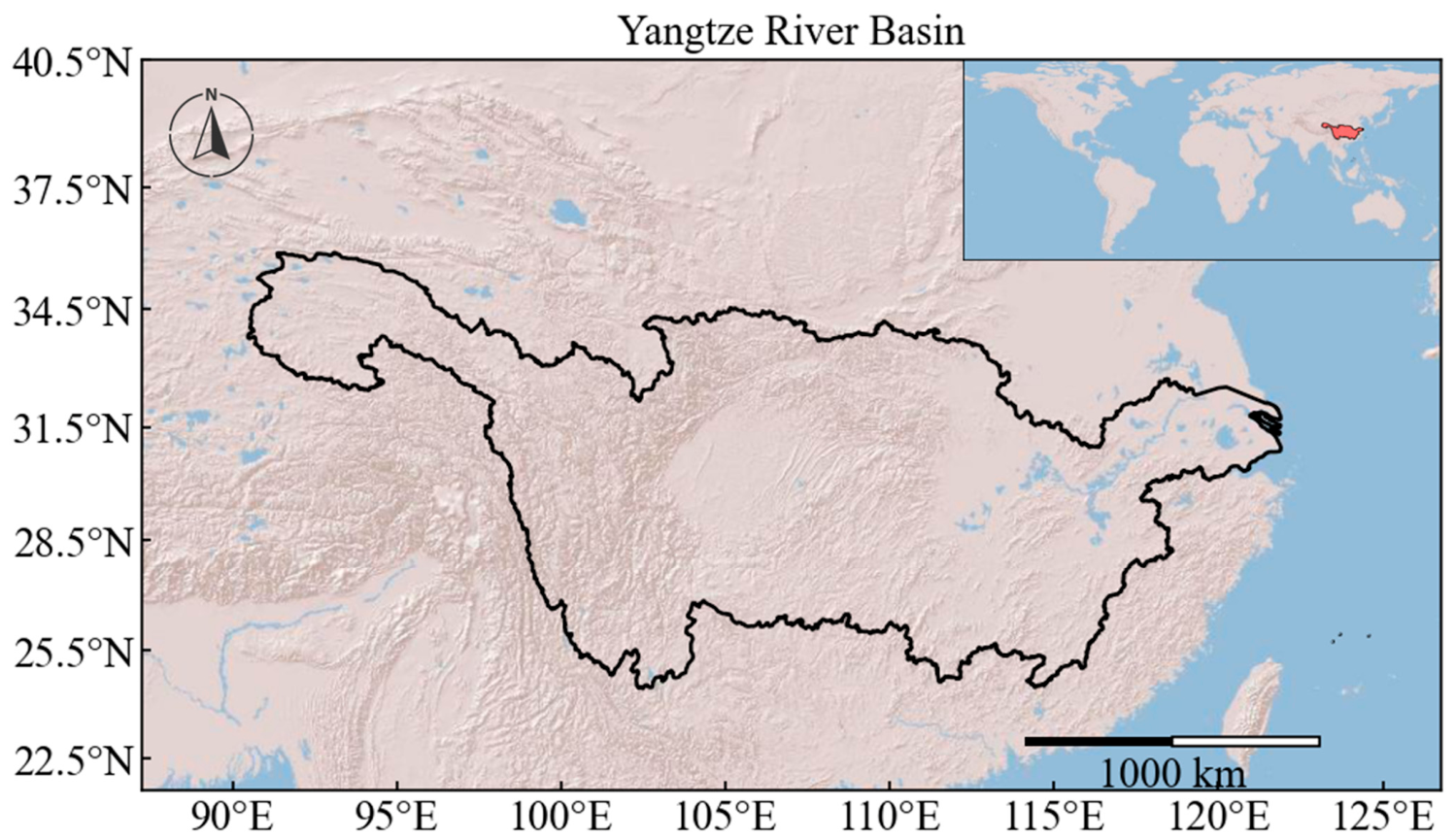
Located in central and eastern China (Figure 1), the YRB spans the eastern, central, and western economic zones of China. Originating east of the Qinghai–Tibet Plateau, the Yangtze River courses through a total of 19 provinces, municipalities, and autonomous regions along its path [28] before emptying into the East China Sea at Shanghai. Geographically, the basin extends from 90°33′E to 122°25′E and from 24°30′N to 35°45′N. The YRB is characterized by highly diverse and complex topography, with terrain gradually descending from the high elevations in the west to the lowlands in the east. Most areas within the basin experience a subtropical monsoon climate, featuring hot and rainy summers and mild, dry winters. The basin possesses abundant water resources, with a dense network of tributaries and numerous lakes. Vegetation in the basin is highly diverse, spanning forest ecosystems (evergreen, deciduous, and mixed), woody savannas, grasslands, croplands, and drylands [22]. These vegetation ecosystems are crucial for ecosystem stability, biodiversity conservation, and regional environmental regulation.

2.2. Data

This study employed multiple datasets, including the drought index (SPEI), structural vegetation indices (EVI, LAI, NDVI), and functional vegetation indicators (GPP, SIF). The SPEI dataset was used to identify drought events, while EVI, LAI, NDVI, GPP and SIF were adopted to calculate post-drought vegetation recovery time. Detailed information on all datasets is summarized in

Table 1. Data information.

Data	Data Source	Time Period	Temporal Resolution	Spatial Resolution
SPEI	SPEIbase v2.10	2000–2023	1 month	0.5°
EVI, NDVI	MOD13Q1	2000–2023	16 days	500 m
LAI	MOD15A2H	2000–2023	8 days	500 m
GPP	PML_V2	2000–2023	8 days	500 m
SIF	LHSIF	2000–2023	1 month	0.05°

. All datasets utilized in this study share the identical spatial reference datum D_WGS_1984.

2.2.1. Drought Index

The SPEI is a widely adopted drought index that integrates rainfall and thermal variables to evaluate the severity and duration of drought conditions in a given region. SPEI quantifies drought by comparing the precipitation–potential evapotranspiration anomalies over a designated time frame with long-term climatological averages, making it a critical tool for drought surveillance, early warning, and risk assessment. SPEI data were derived from SPEIbase v2.10 [29], a global drought dataset. Monthly SPEI values (1901–2023) were calculated using the FAO-56 Penman–Monteith method at 0.5° resolution, covering 1–48 month timescales. The 3-month SPEI data for the period 2000–2023 were extracted from the dataset to investigate the 2022 extreme drought event.

2.2.2. Structural Vegetation Indicators

Structural vegetation indicators reflect canopy morphology, leaf density and vegetation greenness based on surface spectral reflectance features, characterizing the external physical structure of vegetation [30]. In this study, NDVI, EVI and LAI are categorized as structural vegetation indicators.

EVI and NDVI data were primarily obtained from the MOD13Q1 product (https://doi.org/10.5067/MODIS/MOD13Q1.061), a MODIS-based vegetation index dataset developed under the NASA EOS program. The dataset captures global vegetation dynamics through 16-day vegetation index observations at 500 m resolution. In this study, we used data covering the period 2000–2023.

LAI data were obtained from the MOD15A2H product (https://doi.org/10.5067/MODIS/MOD15A2H.061), an 8-day MODIS dataset containing LAI and FPAR information at 500 m resolution for our study period of 2000–2023.

To minimize the impact of cloud cover and low-quality observation data, this study preprocessed the data using quality assurance (QA) information from MODIS products. For the MOD13Q1 NDVI/EVI products, only pixels with a SummaryQA band value of 0 and 1. For the MOD15A2H LAI products, the FparLai_QC band was used to retain only pixels with a MODLAND_QC value of 0 and 1, indicating good quality.

2.2.3. Functional Vegetation Indicators

Functional vegetation indicators directly represent vegetation physiological metabolism and carbon sequestration processes, and quantify instantaneous photosynthetic activity and carbon uptake capacity [31,32]. In this study, GPP and SIF are classified as functional vegetation indicators.

GPP data were obtained from the PML_V2 dataset [33]. Based on the PML model and incorporating stomatal conductance theory, this dataset links evapotranspiration (ET) with GPP processes, providing 8-day data at 500 m resolution for GPP, as well as ET, for the period 2000–2023.

SIF data were obtained from the LHSIF dataset [34], which integrates multi-satellite observations and applies an LUE-based downscaling approach to generate monthly global SIF products at 0.05° resolution during 1995–2023.

2.2.4. Land Cover Data

Land cover data were primarily obtained from the MCD12Q1 dataset (https://doi.org/10.5067/MODIS/MCD12Q1.061), a MODIS-based global land cover dataset generated from Terra and Aqua observations. The product includes multiple land cover classification schemes, such as IGBP and UMD. The data used in this study follow the IGBP classification system, and we used the land cover product for the year 2022.

2.3. Methods

2.3.1. Identification of Extreme Drought Events

(a)

Standardized Anomaly Analysis

Following the approach of Zhang et al. [19], the standardized anomaly index was applied to quantify SPEI-3 anomalies and characterize the spatiotemporal evolution of the 2022–2023 drought in the YRB. The formula is expressed as follows:

$${SA}_{SPEI-3}={\displaystyle \frac{{SPEI}_3^{i,t}-\overline{{SPEI}_3^{i,t}}}{\sigma \left({SPEI}_3^{i,t}\right)}}\left(t=1,2,3\dots 12\right)$$

(1)

where ${SA}_{SPEI-3}$ denotes the SPEI-3 standardized anomaly index, ${SPEI}_3^{i,t}$ represents the SPEI-3 value at pixel i in month t during 2022–2023, $\overline{{SPEI}_3^{i,t}}$ is the corresponding mean over 2000–2023, and $\sigma \left({SPEI}_3^{i,t}\right)$ is its standard deviation over the same period.

(b)

Anomaly Smoothing

Following Saft et al. [35], the standardized anomaly index was smoothed to reduce the influence of isolated wet months on continuous drought conditions. The equation is expressed as:

$$Smoothed{SA}_{SPEI-3}^t={\displaystyle \frac{{SA}_{SPEI-3}^{t-1}+{SA}_{SPEI-3}^t+{SA}_{SPEI-3}^{t+1}}{3}}$$

(2)

where $Smoothed{SA}_{SPEI-3}^t$ denotes the smoothed standardized anomaly index, ${SA}_{SPEI-3}^{t-1}$ represents the value of ${SA}_{SPEI-3}$ for month t − 1 in the 2022–2023 period, ${SA}_{SPEI-3}^t$ denotes the value of ${SA}_{SPEI-3}$ for month t in the 2022–2023 period, and ${SA}_{SPEI-3}^{t+1}$ denotes the value of ${SA}_{SPEI-3}$ for month t + 1 in the 2022–2023 period.

(c)

Identification of Extreme Drought Events

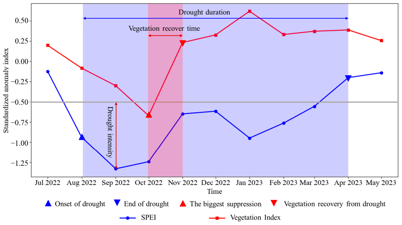
Smoothed ${SA}_{SPEI-3}$ values were adopted to identify drought events with a threshold of −0.5 [19]. Drought onset and termination are defined by threshold crossing, while duration and intensity are derived from event characteristics (Figure 2).

2.3.2. Monitoring Vegetation Recovery Following Extreme Drought

(a)

selection of indicators

A large number of vegetation-related indices have been developed to date, each capable of characterizing different aspects of vegetation [17,30]. This study selected five representative indicators from the perspectives of canopy structure and photosynthetic physiology. NDVI and EVI are classic spectral vegetation indices that both characterize vegetation greenness, but EVI reduces interference from soil and atmospheric noise [30,36,37,38]. LAI represents the total leaf area per unit of ground surface and can intuitively reflect damage to canopy structure following drought [39]. This study also selected two types of vegetation physiological parameters: SIF, which captures photosynthetic activity in real time, and GPP data, which characterize the total amount of accumulated carbon sequestration [40]. These indicators reflect different ecological characteristics during the vegetation recovery process and allow for a comparison of vegetation recovery times following extreme drought from both structural and functional perspectives. Other commonly used indicators, such as PRI and NPP, were not included due to mismatches in spatiotemporal resolution.

(b)

Calculation of Standardized Anomaly Indicators

Standardized anomalies of EVI, NDVI, LAI, GPP, and SIF were calculated to quantify vegetation responses to the extreme drought event:

$${SA}_{EVI}={\displaystyle \frac{x^{i,t}-\overline{x^{i,t}}}{\sigma \left(x^{i,t}\right)}}\left(t=1,2,3\dots 12\right)$$

(3)

$${SA}_{NDVI}={\displaystyle \frac{y^{i,t}-\overline{y^{i,t}}}{\sigma \left(y^{i,t}\right)}}\left(t=1,2,3\dots 12\right)$$

(4)

$${SA}_{LAI}={\displaystyle \frac{z^{i,t}-\overline{z^{i,t}}}{\sigma \left(z^{i,t}\right)}}\left(t=1,2,3\dots 12\right)$$

(5)

$${SA}_{GPP}={\displaystyle \frac{n^{i,t}-\overline{n^{i,t}}}{\sigma \left(n^{i,t}\right)}}\left(t=1,2,3\dots 12\right)$$

(6)

$${SA}_{SIF}={\displaystyle \frac{L^{i,t}-\overline{L^{i,t}}}{\sigma \left(L^{i,t}\right)}}\left(t=1,2,3\dots 12\right)$$

(7)

Here, ${SA}_{EVI}$, ${SA}_{NDVI}$, ${SA}_{LAI}$, ${SA}_{GPP}$ and ${SA}_{SIF}$ denote the standardized anomalies of the corresponding vegetation indicators. Variables $x^{i,t},y^{i,t},z^{i,t},n^{i,t}$ and $L^{i,t}$ represent indicator values at pixel i in month t during 2022–2023. $\overline{x^{i,t}}$,$\overline{y^{i,t}}$,$\overline{z^{i,t}}$,$\overline{n^{i,t}}$ and $\overline{L^{i,t}}$ denote the respective mean values at pixel i in month t from 2000 to 2023. $\sigma \left(x^{i,t}\right)$, $\sigma \left(y\right)$, $\sigma \left(z^{i,t}\right)$, $\sigma \left(n^{i,t}\right)$ and $\sigma \left(L^{i,t}\right)$ denote the standard deviations at pixel i in month t from 2000 to 2023.

(c)

Post-Drought Vegetation Recovery Monitoring

The standardized anomaly indicators of EVI, NDVI, LAI, GPP, and SIF were used to determine the impact of extreme drought on vegetation and to monitor post-drought recovery, following Zhang et al. [19]. We use standardized anomaly values to quantify the intensity of the negative impacts of extreme drought on vegetation. The first month when the standardized anomaly index fell below −0.5 was defined as the onset of negative drought impact on vegetation. The month corresponding to the minimum standardized anomaly index represented the peak drought impact, after which vegetation began to recover. The first month when the standardized anomaly index rose above −0.5 was considered the completion of vegetation recovery. Vegetation recovery time refers to the time interval between the peak of drought-induced vegetation stress and drought recovery completion, as illustrated in Figure 2.

This method results in a downward trend in SPEI anomalies from January to February 2023, while vegetation index anomalies show an upward trend during the same period (Figure 2). This inconsistency may be attributed to seasonal phenological effects. During winter, vegetation in the study area enters a dormant stage, and vegetation activity is relatively limited. As a result, vegetation conditions during this period may show little difference compared with those in normal years [41,42].

3. Results

3.1. Spatiotemporal Characteristics of the 2022 Extreme Drought in the Yangtze River Basin

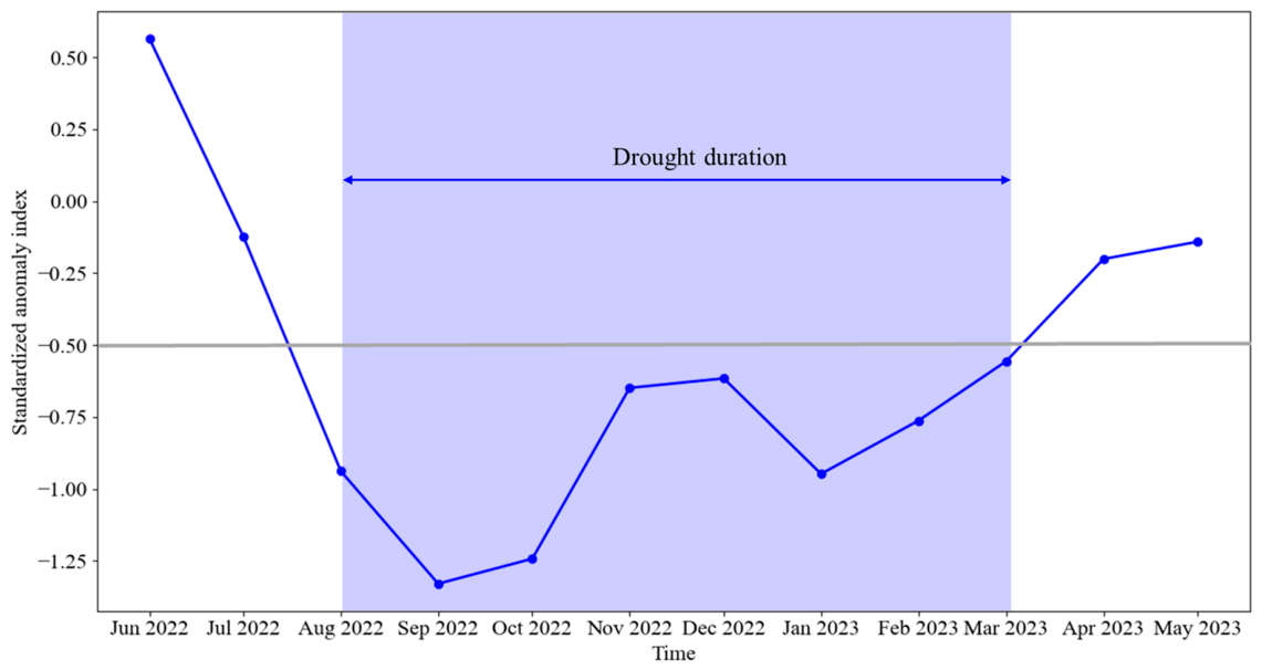
Figure 3 presents the monthly mean ${SA}_{SPEI-3}$ for the YRB from June 2022 to May 2023. The basin-wide mean ${SA}_{SPEI-3}$ first fell below −0.5 in August 2022, indicating the onset of the drought. Following September 2022, the mean ${SA}_{SPEI-3}$ exceeded −0.5 in March 2023, marking the end of the drought. Therefore, this drought event in the YRB mainly occurred between August 2022 and March 2023, with a duration of eight months.

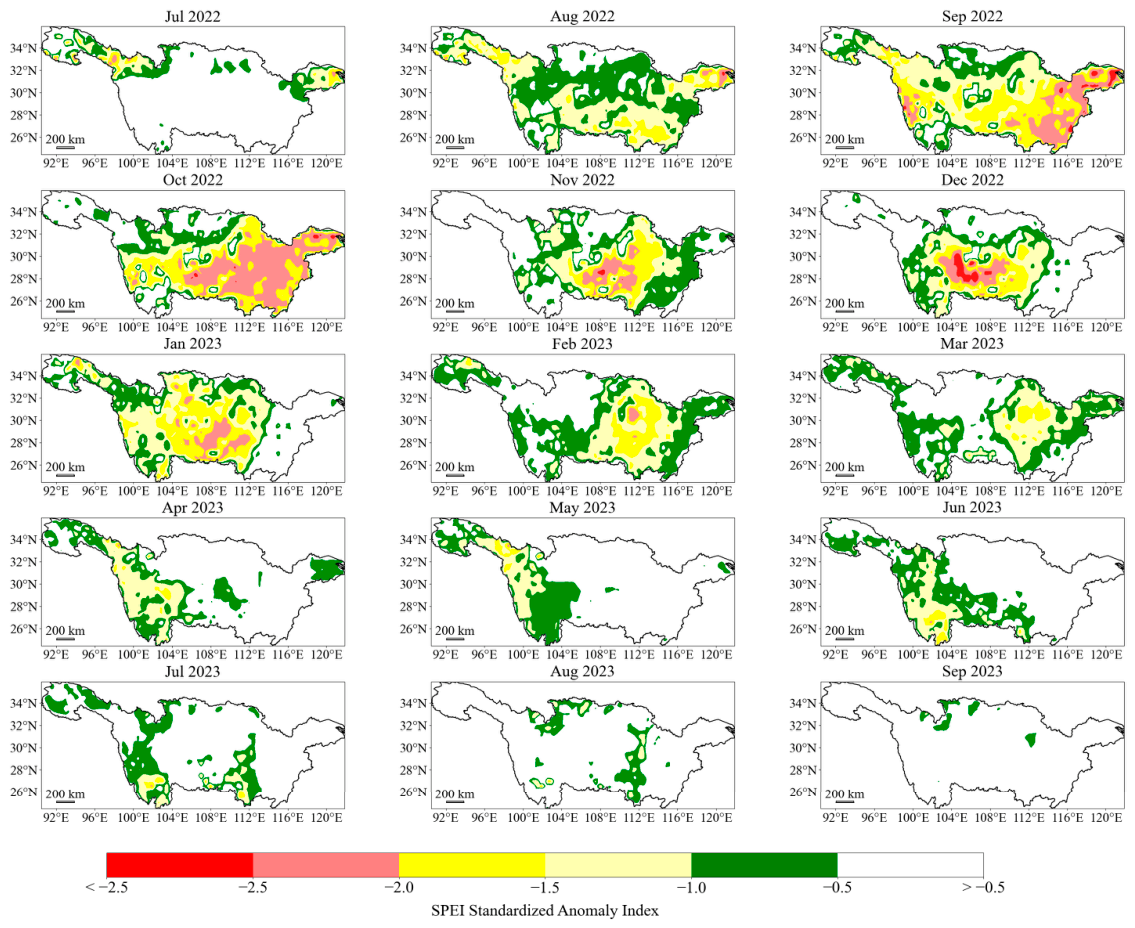
Figure 4 shows the spatial distribution of monthly ${SA}_{SPEI-3}$ across the YRB from June 2022 to September 2023. In August 2022, most parts of the basin were affected by drought. The severity and spatial extent increased in September and October 2022, peaking in October, particularly in the central and eastern regions. Drought conditions then gradually weakened across the basin from November 2022 onwards. During the period from July 2022 to February 2023, some regions exhibited ${SA}_{SPEI-3}$ values below −2, indicating the occurrence of extreme drought, mainly concentrated in the central and eastern parts of the basin.

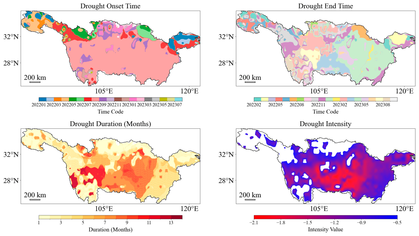
Figure 5 shows the spatial patterns of drought onset, termination, duration, and intensity in 2022. In the northwestern and northeastern regions, drought onset and termination occurred earlier, whereas the central region experienced a later onset and later end. With respect to drought duration, the southwestern part of Sichuan Province and northeastern Yunnan exhibited the longest drought, lasting up to 11 months, while most areas experienced durations of less than 4 months. In terms of drought intensity, severity generally decreased outward from the central region, with the central and southern parts of the basin experiencing the most severe conditions.

3.2. Spatial Patterns and Differences in Vegetation Recovery Time Based on Different Vegetation Indicators

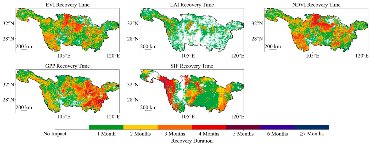
Figure 6 presents the spatial distribution of vegetation recovery time characterized by EVI, LAI, NDVI, GPP, and SIF. Overall, vegetation recovery time derived from all vegetation indicators exhibits a clear spatial correspondence with drought severity, with areas experiencing lower drought intensity showing minimal impact. Base on recovery time derived from EVI, NDVI, and GPP, regions where vegetation remained largely unaffected by drought are mainly located at the junction of Yunnan, Guizhou, and southeastern Sichuan provinces, as well as southern Shaanxi, southwestern Henan, and northeastern Hubei. In contrast, LAI-derived recovery time indicates that more than half of the basin’s vegetation was unaffected by the drought, while recovery time derived from SIF shows unaffected areas mainly in central Sichuan and southwestern Qinghai.

Most vegetation recovered to normal levels within four months after the drought, with the majority recovering in either one or four months. Based on recovery time derived from EVI, LAI, NDVI, and GPP, areas where vegetation recovered within one month were scattered across the basin without a clear spatial pattern. In contrast, SIF-derived recovery time suggests that one-month recovery areas were mainly concentrated in the central and eastern parts of the basin. According to recovery time derived from EVI, NDVI, and GPP, areas requiring four months for vegetation recovery were largely located in southeastern Gansu, northeastern Sichuan, northern Chongqing, southwestern Hubei, southern Sichuan, and northern Yunnan. By comparison, LAI-derived recovery time indicates that four-month recovery areas were primarily in northeastern and western Sichuan, whereas SIF-derived recovery time identifies four-month recovery regions mainly in northwestern Sichuan, southern Qinghai, northwestern Yunnan, southern Gansu, and southern Chongqing. Only a very small portion of the basin required more than five months for vegetation recovery, with no evident spatial pattern. Additionally, SIF-derived recovery time suggests that vegetation in the junction of Sichuan, Guizhou, and Chongqing, as well as southern Jiangxi and southern Anhui, required approximately three months to recover.

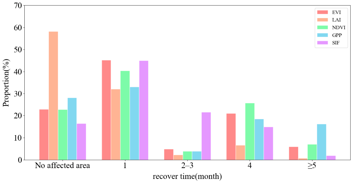
Figure 7 shows the area proportions of the study area that EVI, LAI, NDVI, GPP, and SIF indicate for different vegetation recovery time frames required to return to normal levels. The proportions of drought-unaffected area based on EVI, LAI, NDVI, GPP, and SIF were 22.88%, 58.18%, 22.83%, 28.20%, and 16.49%, respectively, indicating that LAI identifies the largest unaffected area while SIF identifies the smallest.

Recovery time varies across different vegetation indicators. Areas with one-month for recovery time accounted for 45.26%, 32.12%, 40.78%, 33.19%, and 45.06% based on EVI, LAI, NDVI, GPP, and SIF, respectively. Areas requiring 2–3 months for recovery accounted for 4.84%, 2.25%, 3.93%, 3.95%, and 21.63%, and areas requiring four months accounted for 21.06%, 6.65%, 25.69%, 18.51%, and 14.88%, respectively. Areas where recovery required more than five months accounted for 5.97%, 0.79%, 7.35%, 16.25%, and 1.93%, respectively.

Overall, SIF indicates the largest area of vegetation affected by drought, while LAI indicates the smallest. The average recovery time reflected by EVI, LAI, NDVI, GPP, and SIF was 2.23, 1.62, 2.45, 2.79, and 2.00 months, respectively, suggesting that vegetation recovery was fastest according to LAI and slowest according to GPP.

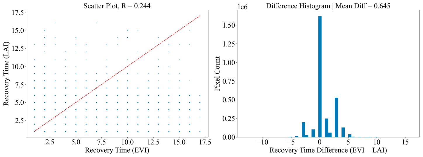
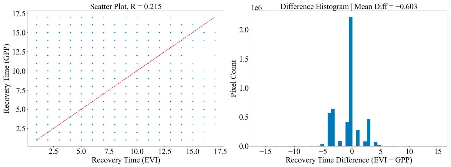
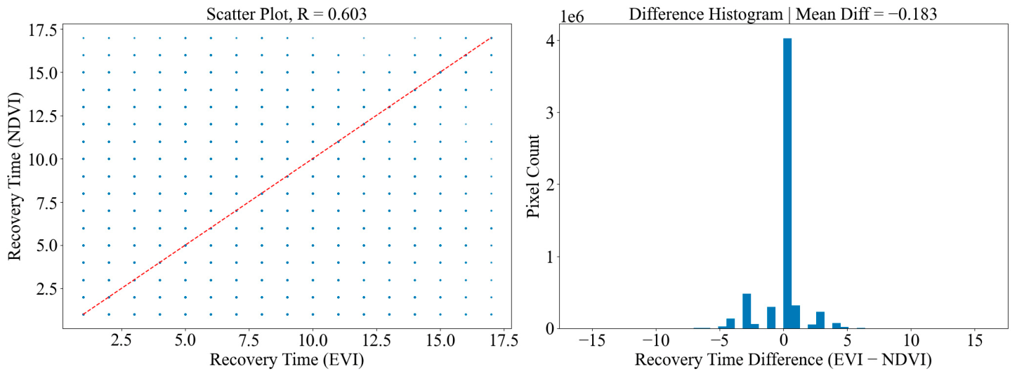
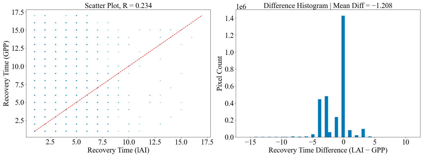
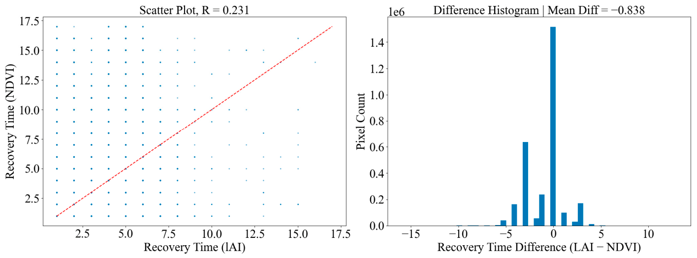
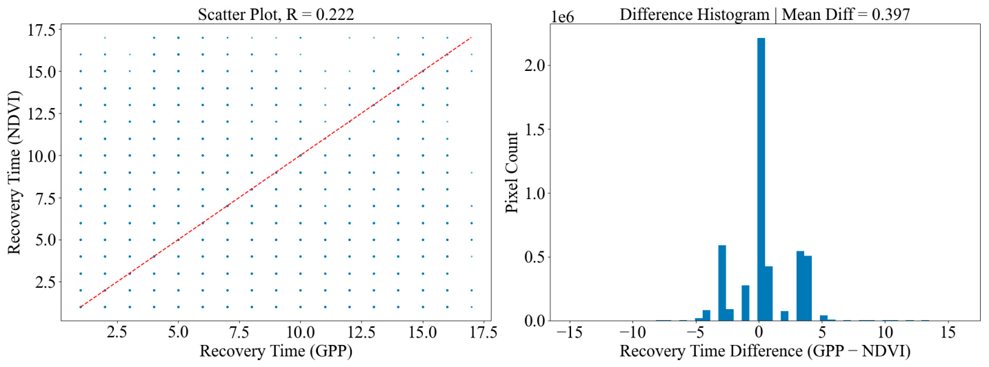
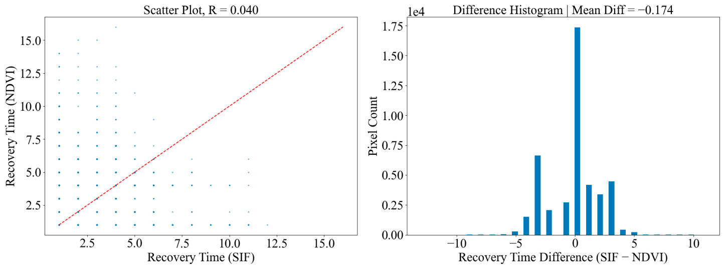
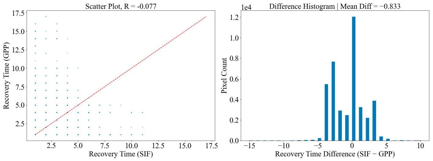
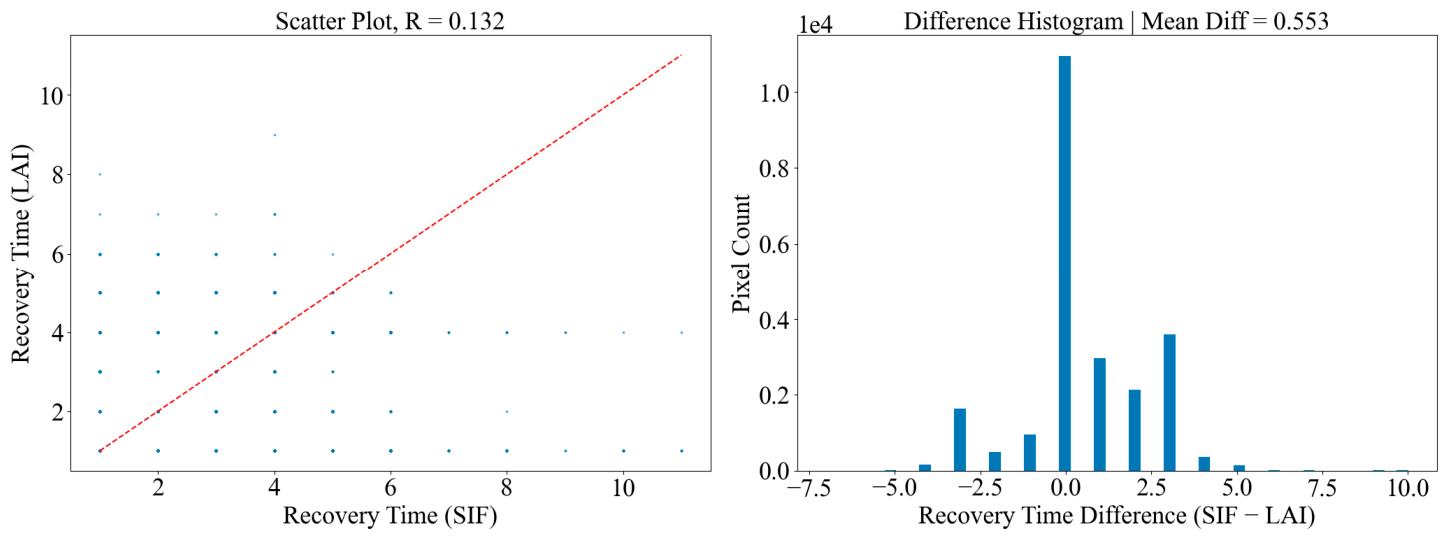
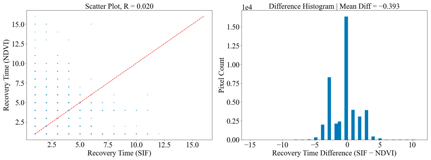
This study further produced scatter plots, difference histograms and corresponding statistical metrics to compare vegetation recovery durations derived from different vegetation indicators (Figure A16, Figure A17, Figure A18, Figure A19, Figure A20, Figure A21, Figure A22, Figure A23, Figure A24 and Figure A25). Among all paired index combinations, EVI and NDVI achieved the highest Pearson correlation coefficient (R = 0.603), with a small mean difference of −0.1831 (Figure A17), as well as relatively low mean absolute error (MAE) and root mean square error (RMSE). This result indicates minimal divergence in vegetation recovery time captured by EVI and NDVI. In contrast, all paired groups involving GPP exhibited correlation coefficients below 0.24 and RMSE values greater than 2.0, revealing substantial disparities between recovery durations quantified by GPP and the other four indicators. Extremely weak correlations were detected between SIF and LAI, EVI and NDVI, with R values ranging from 0.02 to 0.13 (Figure A22, Figure A23, Figure A24 and Figure A25). Among these pairs, SIF and NDVI showed the weakest correlation at R = 0.02. Paired sample t-tests were conducted for each pairwise index comparison, and all resulting p-values approximated zero, demonstrating statistically significant differences in the quantification of vegetation recovery duration across distinct biophysical indicators. Overall, EVI and NDVI presented the strongest correlation and the smallest discrepancies in recovery time estimation, whereas SIF and NDVI displayed the weakest correlation and the most remarkable divergences.

3.3. Recovery Time Across Vegetation Types

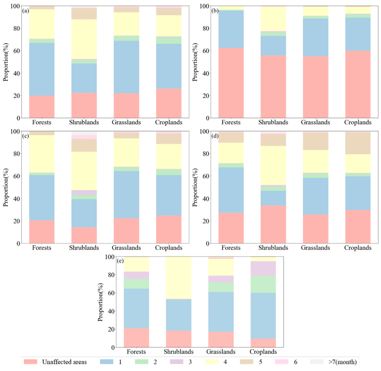
Figure 8 present the proportion of forest, shrub, grassland, and cropland areas recovering to normal levels, as reflected by EVI, LAI, NDVI, GPP, and SIF. According to EVI, LAI, and GPP, forests exhibit the fastest recovery, with average recovery time of 2.20, 1.31, and 2.40 months, respectively. The proportion of forest areas recovering within one month based on the three indicators was 46.94%, 33.23%, and 40.48%, respectively. In contrast, NDVI indicated that grasslands recovered the fastest after the extreme drought, with nearly half of grassland areas recovering within one month (43.02%), and an average recovery time of 2.40 months. Consistent with EVI, LAI, and GPP, NDVI also indicated rapid forest recovery, with 40.22% of forest areas recovering within one month and an average recovery time of 2.48 months, slightly slower than grasslands by 0.08 months. SIF suggested that croplands had the fastest recovery, with 50.40% of cropland areas recovering within one month and an average recovery time of 1.75 months.

For all vegetation indicators, shrubs exhibited the slowest post-drought recovery. The proportion of shrub areas recovering in four months exceeded that recovering in one month, and the average recovery times were 3.13, 2.70, 3.41, 3.56, and 2.73 months according to EVI, LAI, NDVI, GPP, and SIF, respectively.

4. Discussion

4.1. Reasons for Differences in Vegetation Recovery Times as Reflected by Various Vegetation Indicators

Our study shows that the vegetation recovery times derived from different vegetation indicators was significantly different, indicating that the indicators capture vegetation recovery in distinct ways. Average recovery times based on EVI, LAI, NDVI, GPP, and SIF were 2.23, 1.62, 2.45, 2.79, and 2.00 months, respectively. LAI indicated the shortest recovery time, followed by SIF, EVI, NDVI, and GPP, while GPP reflected the longest recovery time, consistent with Zhang et al. [19]. These differences arise from the distinct vegetation information captured by each index.

LAI, defined as the total leaf area per unit ground area, characterizes canopy structure and energy absorption capacity [39]. Following extreme drought, although plants are affected, leaves may remain intact and the total leaf area is less impacted. As a result, LAI tends to reflect the fastest vegetation recovery. SIF, as an effective probe of photosynthesis [40], reflects actual photosynthetic activity [43,44]. After drought, leaves may persist while photosynthesis can be severely inhibited. Therefore, SIF reveals a longer recovery time than LAI.

NDVI and EVI assess vegetation by measuring the reflectance of leaves in the near-infrared and red spectral bands, representing leaf structure and chlorophyll content [30,36,37,38], which indirectly reflects photosynthetic capacity. Consequently, the recovery times indicated by EVI and NDVI are similar. Since the restoration of photosynthetic rates precedes the recovery of leaf structure and chlorophyll content, EVI and NDVI typically indicate longer recovery times than SIF.

GPP quantifies the total carbon assimilated by vegetation through photosynthesis over a given spatial and temporal scale [45,46,47]. The longer recovery time reflected by GPP may be attributed to the fact that total carbon fixation is the end result of photosynthesis, and its recovery depends on both photosynthetic rate and the restoration of leaf structure and chlorophyll content, requiring more time than indicators that directly measuring these components [48,49].

Furthermore, intrinsic structural discrepancies between datasets lead to divergent recovery durations inferred from GPP and SIF. The PML_V2 model for GPP simulation is a coupled evapotranspiration–carbon biophysical framework heavily constrained by meteorological forcing inputs, including precipitation, air temperature, and vapor pressure deficit [33]. Severe drought creates persistent deep soil moisture deficits, and soil moisture anomalies exhibit significant climate memory, requiring multiple consecutive wet months to restore long-term climatological averages [50]. Meanwhile, large-scale warm atmospheric circulation persists long after the drought subsides, keeping the vapor pressure deficit (VPD) elevated for months and continuously limiting vegetation stomatal conductance and transpiration [51]. Such a delayed recovery of meteorological drivers directly propagates into GPP simulations, introducing systematic temporal delays in modeled productivity time series. In contrast, the LHSIF SIF dataset is derived directly from satellite hyperspectral radiance without coupling to meteorological models, enabling it to capture canopy recovery signals immediately once water stress is alleviated [40,44].

Different vegetation indicators capture different aspects of vegetation status, and their effectiveness varies depending on the research objectives. In this study, multiple vegetation indicators were compared to evaluate post-drought recovery across vegetation types. In future research, appropriate indicators can be selected based on specific research objectives to further investigate post-drought vegetation recovery dynamics.

4.2. Factors Influencing Recovery Time Differences Among Different Vegetation Types

Au et al. found that forests generally exhibit rapid post-drought recovery due to their extensive canopy and leaf coverage, as well as deep root systems enabling water uptake from deeper soil layers [52]. These characteristics confer drought resistance by maintaining water retention during drought events [53], and enable rapid leaf regrowth after the drought ends. EVI, LAI, and GPP all indicate that forests recover relatively quickly, consistent with previous findings [19,54].

In contrast, Grasslands are characterized by a simpler structure, higher vegetation density, and shorter growth cycles, which contributed to relatively rapid recovery following drought [19]. Consequently, NDVI reflects rapid post-drought recovery in grasslands, consistent with prior research [15,16]. Croplands are strongly influenced by human management, and agricultural interventions can accelerate recovery after extreme drought events. SIF, as an accurate proxy for actual photosynthetic activity [55], can capture the restoration of photosynthetic rates even before the greenness of crops fully recovers, explaining why SIF indicates the fastest recovery in croplands. This result is consistent with the results reported by Han et al. [56]. Shrubs, however, have a relatively simple structure and shallow root systems, making them more vulnerable to drought [57]. During drought, reduced shallow soil moisture restricts shrub growth, prolonging recovery periods [14]. As a result, EVI, LAI, NDVI, GPP, and SIF consistently indicate that shrubs exhibit the slowest post-drought recovery.

Differences in ecological conditions, methodological approaches, and selected vegetation indicators may contribute to inconsistencies in existing studies on post-drought vegetation recovery. Future research is needed to provide a more comprehensive understanding of vegetation recovery dynamics following extreme drought events.

4.3. Threshold Sensitivity Analysis of Vegetation Recovery Duration

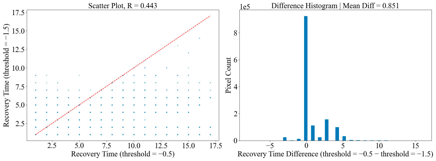
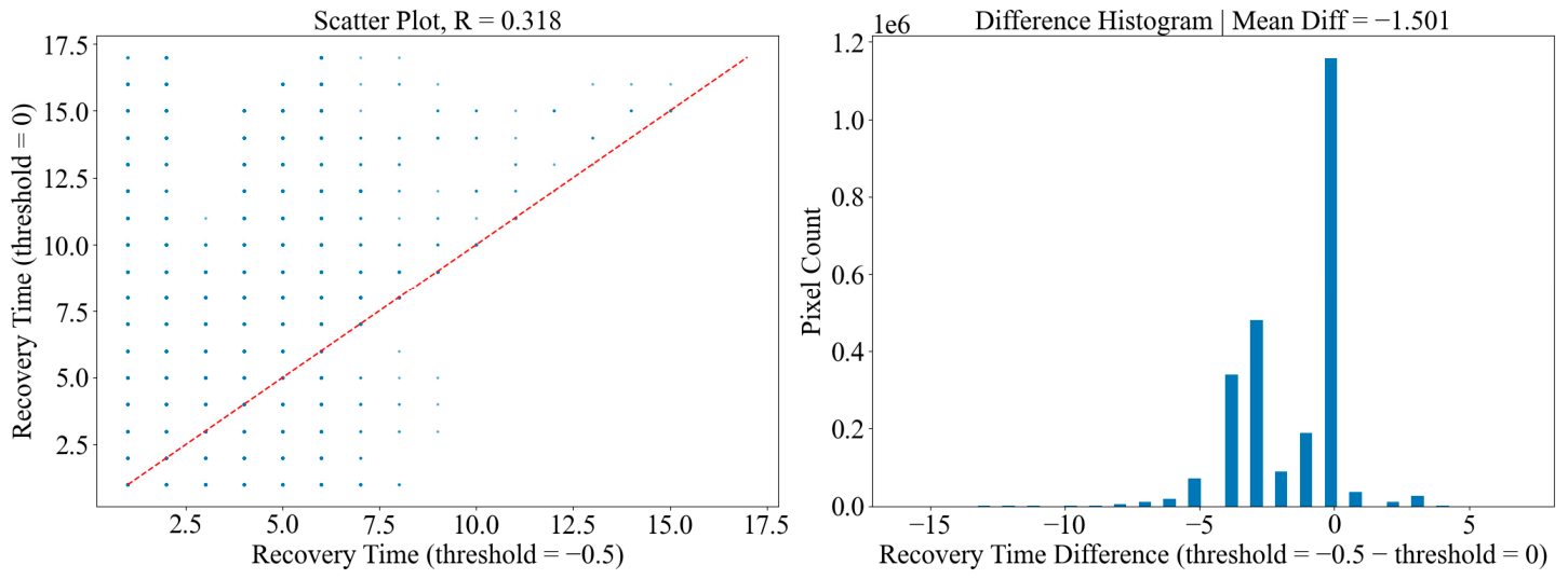
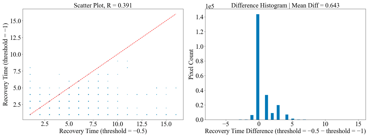
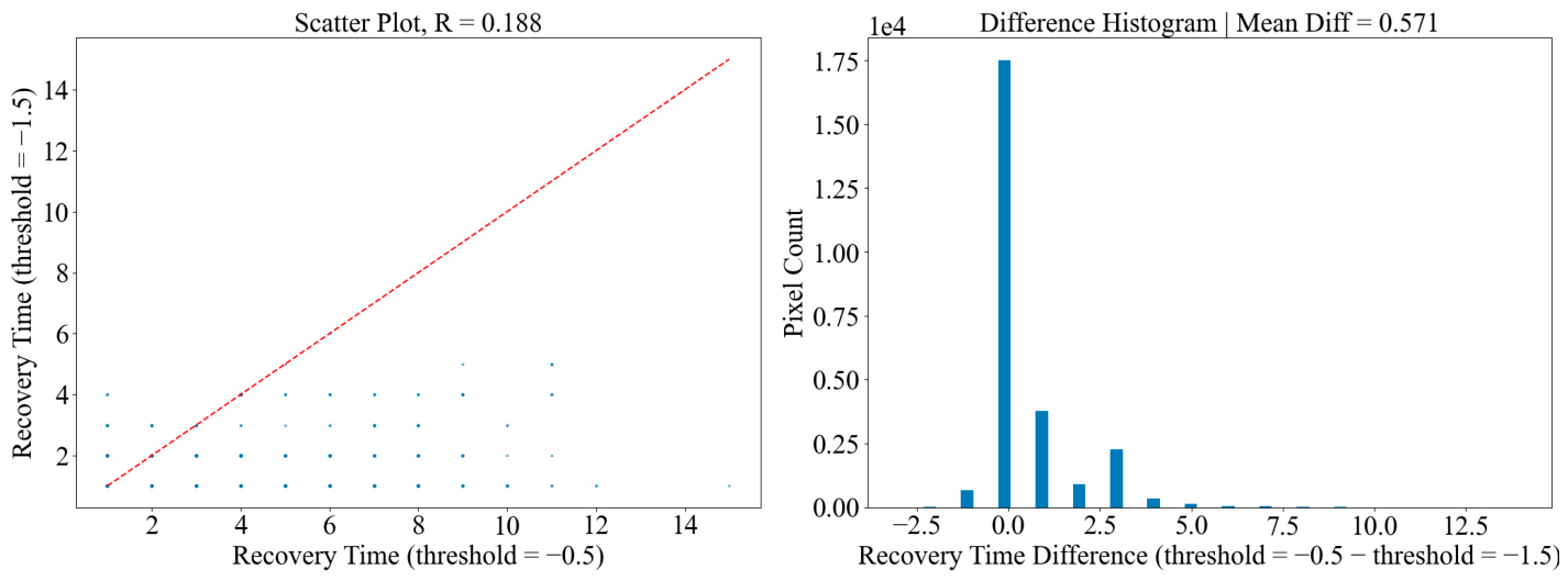
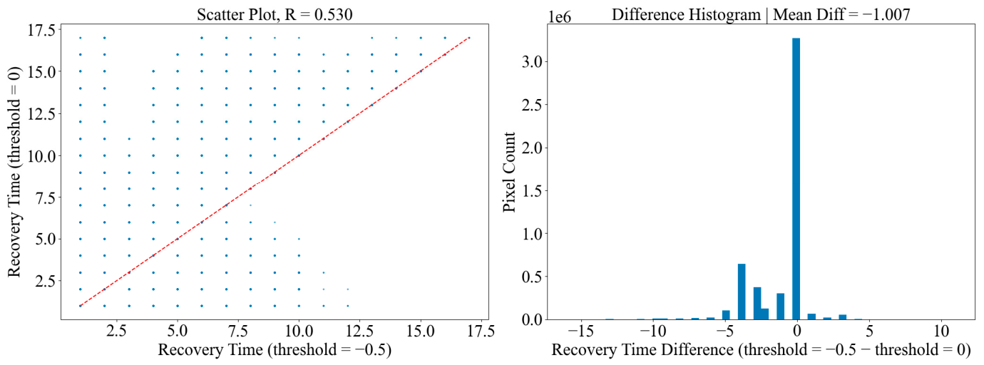
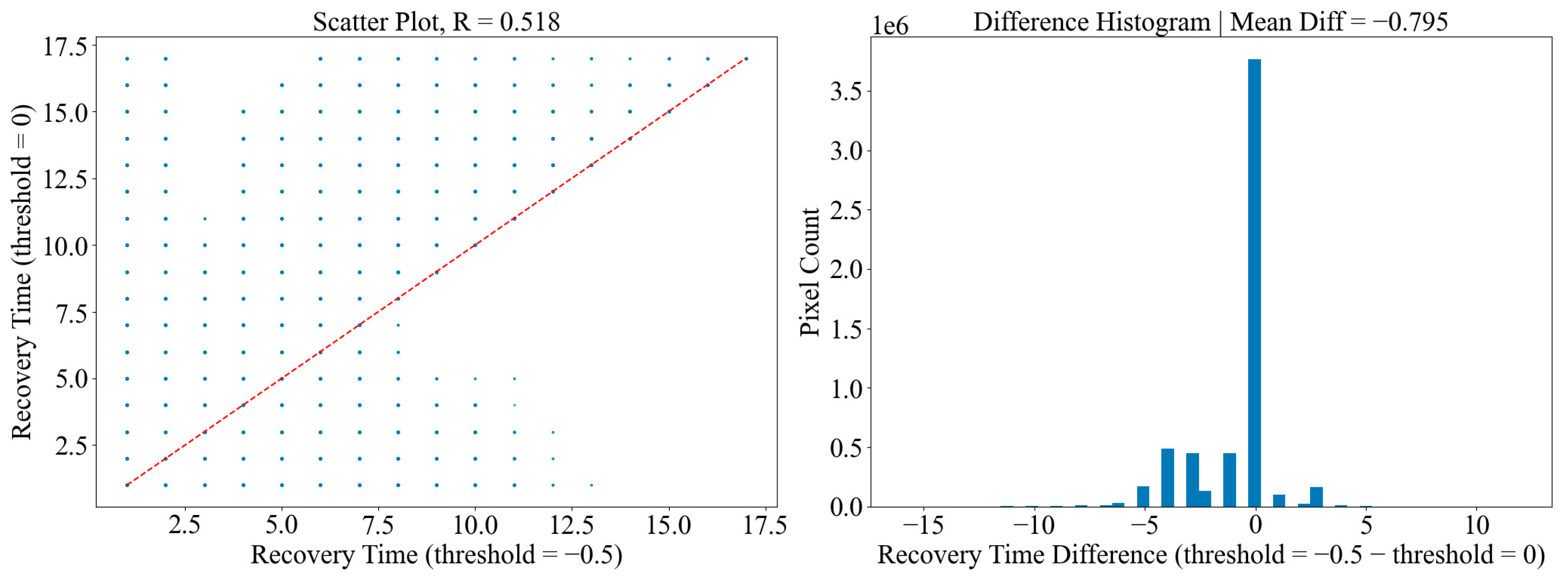
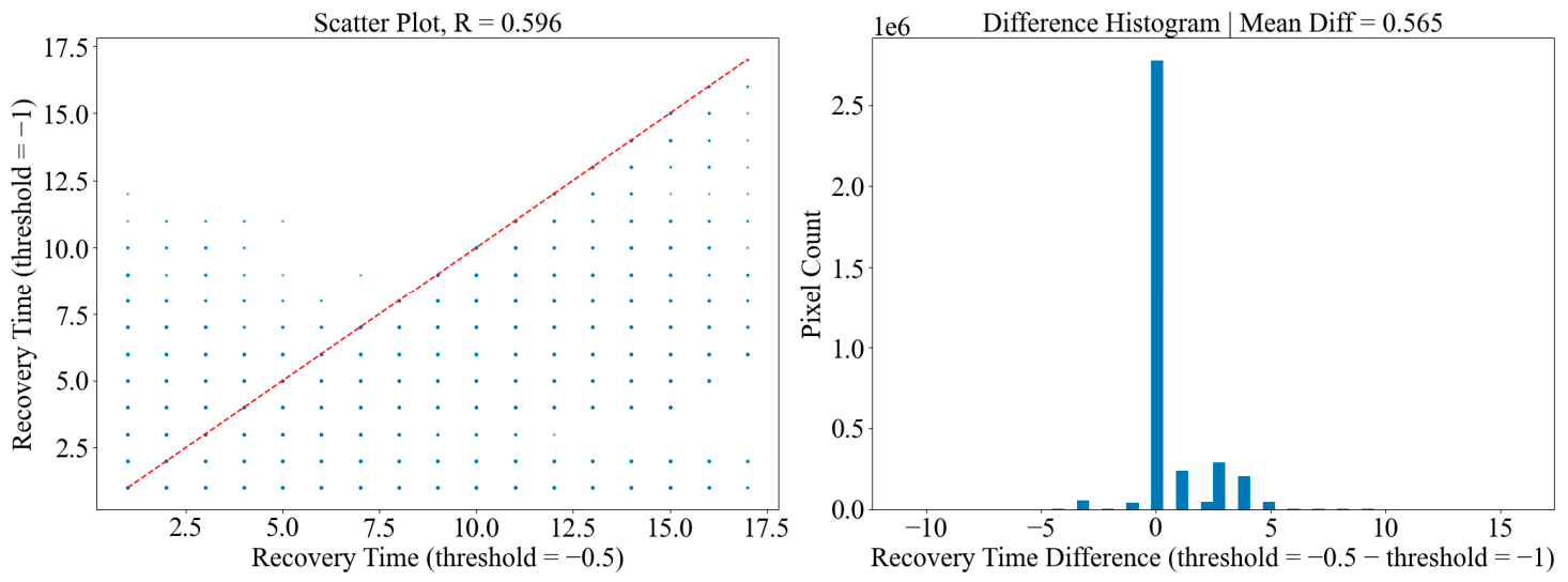
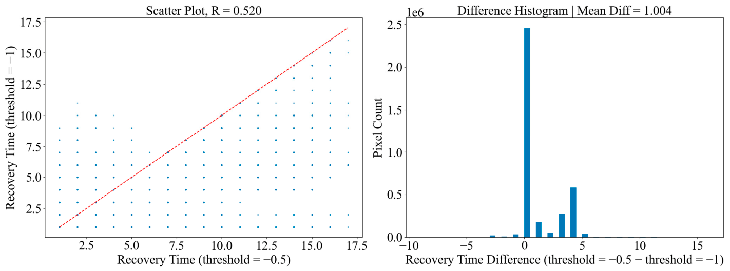
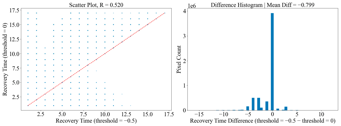
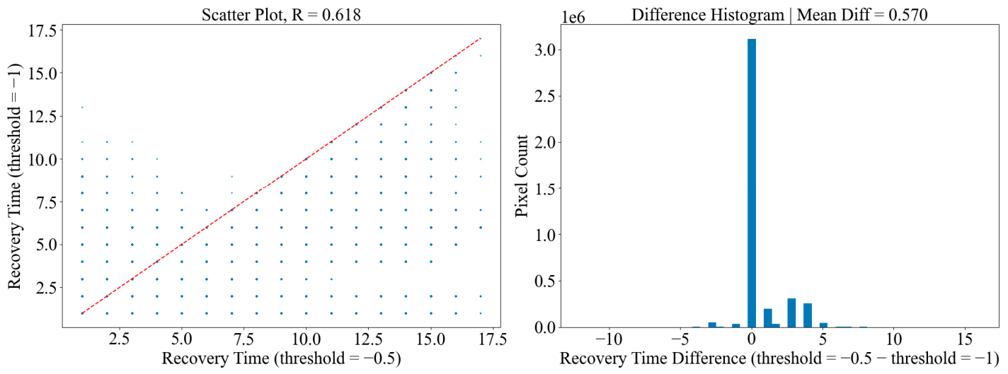
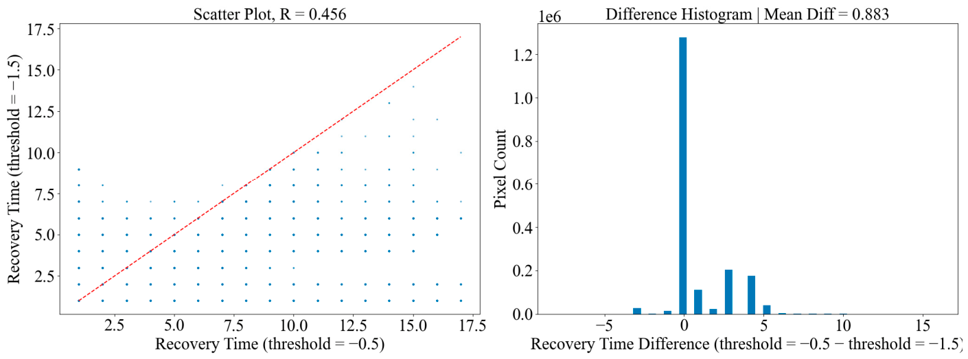
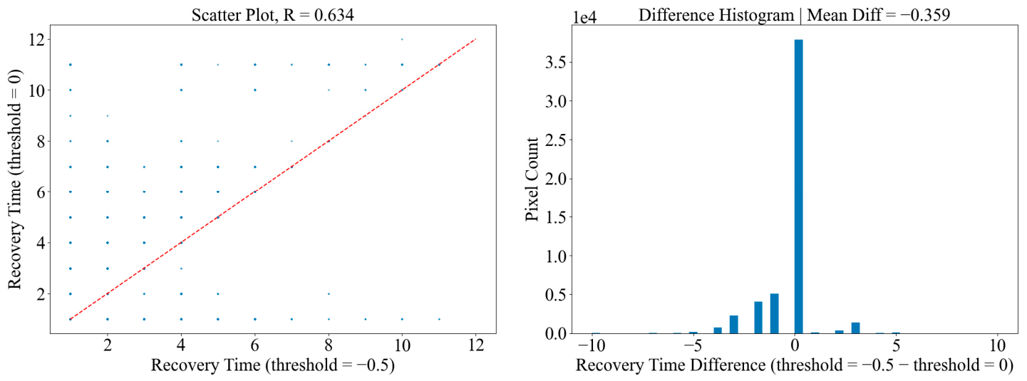
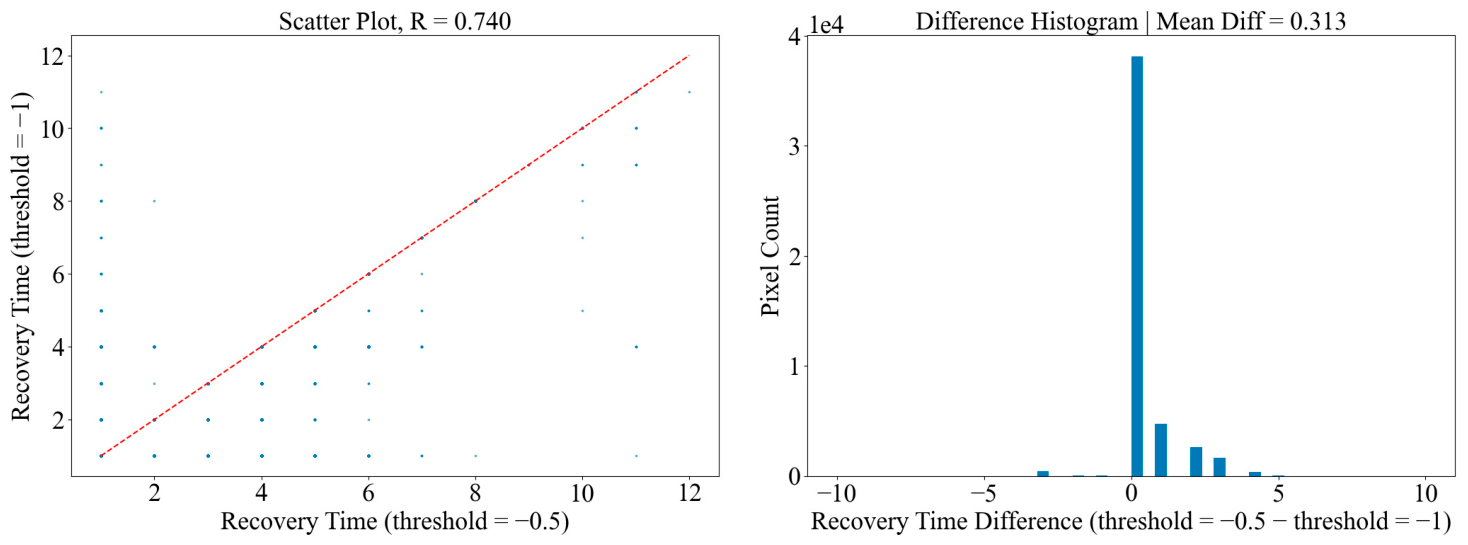
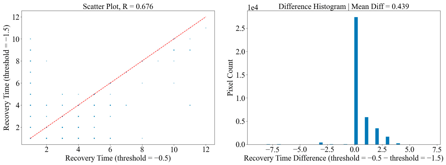
This study uses a standardized outlier value of −0.5 as the reference threshold to calculate the vegetation recovery time as reflected by five indicators: EVI, LAI, NDVI, GPP, and SIF. To discuss the uncertainty associated with using a single fixed threshold and to verify the robustness of the vegetation recovery time calculated based on the reference threshold, this study additionally calculated vegetation recovery times using three sets of thresholds (0, −1.0, and −1.5) and employed paired t-tests, Pearson correlation analysis, mean differences, mean absolute error (MAE), and root mean square error (RMSE) to compare the differences in vegetation recovery times calculated using different thresholds (Figure A1, Figure A2, Figure A3, Figure A4, Figure A5, Figure A6, Figure A7, Figure A8, Figure A9, Figure A10, Figure A11, Figure A12, Figure A13, Figure A14 and Figure A15). The histograms of differences for all indicators show that the number of pixels where the difference equals 0 represents the global peak. This result indicates that the drought stress intensity of most pixels in the study area is far from the critical ranges of each threshold; adjusting the classification criteria does not alter the vegetation recovery time assessments for these areas, and the overall recovery time pattern derived from the −0.5 threshold exhibits fundamental stability. However, the histograms also show a large number of discrete pixels with positive and negative differences, and the p-values from paired t-tests for each group all approach 0. This indicates that the magnitude of recovery time shifts within drought-sensitive critical zones is sufficient to cause systematic estimation biases across the entire study area; relying solely on a single fixed threshold cannot completely eliminate this uncertainty.

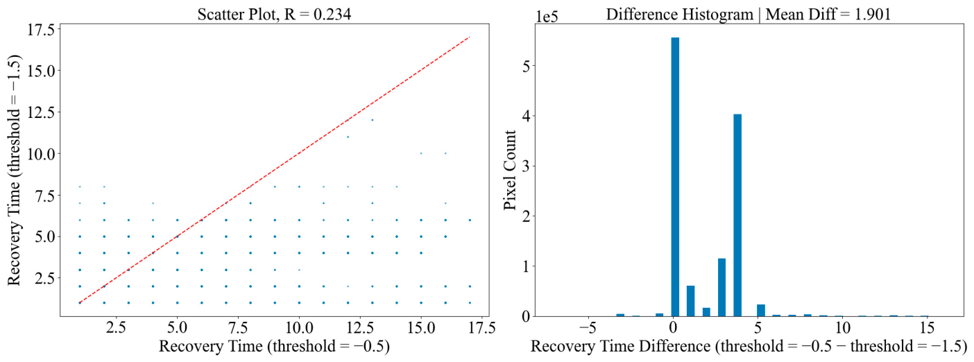
This study considers a threshold of 0 to be a lenient threshold and a threshold of −1.5 to be a strict threshold. The lenient threshold results in a longer estimated vegetation recovery time, while the strict threshold shortens the estimated recovery time. The sensitivity of different indicators to threshold variations differs significantly, with the sensitivity ranked as follows: GPP > LAI > NDVI ≈ EVI > SIF. The GPP group exhibited the largest difference in mean values between thresholds (a difference of 1.9010 between −0.5 and −1.5), a weak correlation coefficient (R = 0.234) (Figure A7, Figure A8 and Figure A9), and the highest MAE and RMSE values, indicating that the model’s simulated GPP results are highly susceptible to the choice of threshold. This may be partly because the PML_V2 GPP product incorporates satellite observations, meteorological variables, and evapotranspiration-related processes, which may increase the variability of GPP anomalies and their sensitivity to threshold selection [58,59]. As green vegetation indicators, the results of the threshold difference analysis for NDVI and EVI were highly consistent, with moderate intergroup variations (Figure A1, Figure A2, Figure A3, Figure A10, Figure A11 and Figure A12); LAI also exhibited strong sensitivity, with a mean difference of −1.5007 between the −0.5 and 0 thresholds (Figure A4, Figure A5 and Figure A6). In contrast, SIF exhibited the smallest mean differences across threshold groups, the highest overall Pearson correlation coefficients (0.634–0.740) (Figure A13, Figure A14 and Figure A15), and the lowest error metrics across all groups, demonstrating that SIF provides more robust results regarding vegetation recovery time and is subject to less uncertainty due to threshold selection.

4.4. Limitations of This Study

Although this study used multi-source remote sensing indicators to assess vegetation recovery times following the extreme drought event in the Yangtze River Basin in 2022, several limitations remain. First, differences in spatial resolution among the various datasets may introduce uncertainty into the estimates of vegetation recovery times. The vegetation remote sensing indicators and land cover data used in this study both have a spatial resolution of 500 m, whereas the SIF data have a spatial resolution of 0.05°. In this study, NDVI, EVI, LAI, and GPP products (500 m) were resampled to 0.05° using the spatial averaging aggregation method to match the spatial resolution of the SIF product before pixel-wise correlation analysis. During this upscaling process, a large number of pixels with differing recovery statuses were averaged into the same coarse grid, smoothing out the fine-scale spatial heterogeneity of vegetation recovery and thereby weakening the correlation between NDVI, EVI, LAI, GPP, and SIF [60,61]. At the same time, extreme values of standardized vegetation negative anomalies were neutralized and compressed during this process, the recovery time for pixels experiencing severe drought was shortened, and the statistical variation in recovery times across different vegetation indicators was reduced [30].

In addition, the insufficient spatial resolution of the dataset may also introduce bias in the calculation of recovery times. Since a single remote sensing pixel typically contains various surface components—such as multiple vegetation types, bare soil, and water bodies—the mixed-pixel effect may reduce the sensitivity of remote sensing indicators to local vegetation changes [61]. Furthermore, data with coarser spatial resolution tend to reduce landscape heterogeneity during spatial aggregation, smoothing out small-scale spatial variations in drought impacts and recovery processes, and making it difficult to accurately capture the responses of local ecological units such as microtopography, small forested patches, and scattered farmland [60]. Therefore, future research could integrate higher-resolution remote sensing data with multiscale analytical methods to further improve the ability to characterize the spatiotemporal heterogeneity of vegetation recovery following extreme droughts.

Second, this study adopted the method proposed by Zhang et al., using a fixed standardized anomaly threshold (−0.5) to determine the time of complete vegetation recovery [19]; this method has been widely applied in studies of drought impacts and ecological recovery [15,16]. However, estimates of recovery time are typically sensitive to the choice of anomaly threshold, and different thresholds may lead to overestimation or underestimation of recovery duration, particularly across different vegetation functional types and ecological process indicators [9]. Although this study validated the stability of the results through multi-threshold sensitivity analysis, a single threshold still cannot fully reflect the different physiological recovery processes represented by indicators such as NDVI, EVI, LAI, SIF, and GPP. Therefore, future research should further explore dynamic recovery thresholds based on ecosystem types and the characteristics of remote sensing indicators to reduce estimation biases resulting from threshold selection.

5. Conclusions

This study employed multiple vegetation indicators, including the SPEI, NDVI, EVI, LAI, GPP, and SIF, to investigate vegetation recovery following the extreme drought in the YRB in 2022. We found that most vegetation recovered within one month, followed by areas requiring four months for recovery. The average recovery times indicated by EVI, LAI, NDVI, GPP, and SIF were 2.23, 1.62, 2.45, 2.79, and 2.00 months, respectively, with LAI reflecting the shortest recovery time and GPP the longest. Regarding vegetation types, EVI, LAI, and GPP reflected the fastest post-drought recovery in forests and the slowest in shrubs; NDVI indicated the fastest recovery in grasslands and the slowest in shrubs; SIF showed the fastest recovery in croplands and the slowest in shrubs. Overall, forests and grasslands recovered relatively quickly, whereas croplands and shrubs exhibited slower recovery.

Our findings provide quantitative and qualitative analyses of this extreme drought event, with different vegetation indicators reflecting post-drought recovery timelines. These findings provide guidance for drought risk management, vegetation index selection, and ecological restoration in arid regions, while also supporting sustainable agricultural production, socio-economic development, and ecosystem stability.

References

1. Pan, S.; He, Z.; Chen, L.; Wang, M. Spatiotemporal Evolution Characteristics of Meteorological Drought in Guizhou Province in Recent 50 Years Based on Different Time Scales. Res. Soil Water Conserv. 2023, 30, 279–288. [Google Scholar] [CrossRef]
2. Li, J.P.; Chen, L.J.; Zhang, G.L.; Liu, H.; Hu, H.C.; Xu, M.Z.; Guo, X.Y.; Meng, Z.B.; Dong, Z.Q. Identification and characterization of long-term meteorological drought events in the Yellow River Basin. Ecol. Inform. 2025, 86, 102992. [Google Scholar] [CrossRef] [Scilit]
3. IPCC. Climate Change 2021—The Physical Science Basis: Working Group I Contribution to the Sixth Assessment Report of the Intergovernmental Panel on Climate Change; Cambridge University Press: Cambridge, UK, 2023. [Google Scholar] [CrossRef] [Scilit]
4. Vanoni, M.; Bugmann, H.; Nötzli, M.; Bigler, C. Drought and frost contribute to abrupt growth decreases before tree mortality in nine temperate tree species. For. Ecol. Manag. 2016, 382, 51–63. [Google Scholar] [CrossRef] [Scilit]
5. Bastos, A.; Gouveia, C.M.; Trigo, R.M.; Running, S.W. Analysing the spatio-temporal impacts of the 2003 and 2010 extreme heatwaves on plant productivity in Europe. Biogeosciences 2014, 11, 3421–3435. [Google Scholar] [CrossRef] [Scilit]
6. De Boeck, H.J.; Dreesen, F.E.; Janssens, I.A.; Nijs, I. Whole-system responses of experimental plant communities to climate extremes imposed in different seasons. New Phytol. 2011, 189, 806–817. [Google Scholar] [CrossRef] [Scilit] [PubMed]
7. Wang, C.Y.; Chen, J.; Lee, S.C.; Xiong, L.H.; Su, T.H.; Lin, Q.; Xu, C.Y. Response and recovery times of vegetation productivity under drought stress: Dominant factors and relationships. J. Hydrol. 2025, 655, 132945. [Google Scholar] [CrossRef] [Scilit]
8. Zhang, Y.; Liu, X.H.; Jiao, W.Z.; Wu, X.C.; Zeng, X.M.; Zhao, L.J.; Wang, L.X.; Guo, J.Q.; Xing, X.Y.; Hong, Y.X. Spatial Heterogeneity of Vegetation Resilience Changes to Different Drought Types. Earth’s Future 2023, 11, e2022EF003108. [Google Scholar] [CrossRef] [Scilit]
9. Lloret, F.; Keeling, E.G.; Sala, A. Components of tree resilience: Effects of successive low-growth episodes in old ponderosa pine forests. Oikos 2011, 120, 1909–1920. [Google Scholar] [CrossRef] [Scilit]
10. Simoniello, T.; Lanfredi, M.; Liberti, M.; Coppola, R.; Macchiato, M. Estimation of vegetation cover resilience from satellite time series. Hydrol. Earth Syst. Sci. 2008, 12, 1053–1064. [Google Scholar] [CrossRef] [Scilit]
11. Wang, H.C.; Zhu, Q.; Wang, Y.S.; Zhang, H. Spatio-temporal characteristics and driving factors of flash drought recovery: From the perspective of soil moisture and GPP changes. Weather Clim. Extrem. 2023, 42, 100605. [Google Scholar] [CrossRef] [Scilit]
12. Hao, Y.; Baik, J.; Fred, S.; Choi, M. Comparative analysis of two drought indices in the calculation of drought recovery time and implications on drought assessment: East Africa’s Lake Victoria Basin. Stoch. Environ. Res. Risk Assess. 2022, 36, 1943–1958. [Google Scholar] [CrossRef] [Scilit]
13. Vo, Q.T.; So, J.M.; Bae, D.H. An Integrated Framework for Extreme Drought Assessments Using the Natural Drought Index, Copula and Gi* Statistic. Water Resour. Manag. 2020, 34, 1353–1368. [Google Scholar] [CrossRef] [Scilit]
14. Lu, X.J.; Dong, S.L.; Yan, H.B.; Zhao, T.J.; Zhao, F.Y.; Xu, F.J. Quantifying global vegetation recovery speed in response to extreme drought using multi-dimensional spatiotemporal data. Int. J. Digit. Earth 2025, 18, 2507195. [Google Scholar] [CrossRef] [Scilit]
15. Wu, C.H.; Zhong, L.L.; Yeh, P.J.F.; Gong, Z.J.; Lv, W.H.; Chen, B.; Zhou, J.; Li, J.Y.; Wang, S.S. An evaluation framework for quantifying vegetation loss and recovery in response to meteorological drought based on SPEI and NDVI. Sci. Total Environ. 2024, 906, 167632. [Google Scholar] [CrossRef] [Scilit] [PubMed]
16. Yao, Y.; Fu, B.J.; Liu, Y.X.; Li, Y.; Wang, S.; Zhan, T.Y.; Wang, Y.J.; Gao, D.X. Evaluation of ecosystem resilience to drought based on drought intensity and recovery time. Agric. For. Meteorol. 2022, 314, 108809. [Google Scholar] [CrossRef] [Scilit]
17. Yang, T.; Qin, J.; Li, X.; Zhou, X.; Lu, Y. Ecological and vegetation responses in a humid region in southern China during a historic drought. J. Environ. Manag. 2024, 371, 122986. [Google Scholar] [CrossRef] [Scilit] [PubMed]
18. Liu, P. Inaugural Editorial for the Journal of Geoscience and Earth Observation. J. Geosci. Earth Obs. 2025, 1, 1–3. [Google Scholar] [CrossRef] [Scilit]
19. Zhang, Y.; Gu, T.; He, S.; Cheng, F.; Wang, J.; Ye, H.; Zhang, Y.; Su, H.; Li, Q. Extreme drought along the tropic of cancer (Yunnan section) and its impact on vegetation. Sci. Rep. 2024, 14, 7508. [Google Scholar] [CrossRef] [Scilit] [PubMed]
20. Liu, S. The Core Essence, Underlying Methodology, and Innovative Contributions of General Secretary Xi Jinping’s Important Discourse on Promoting the Development of the Yangtze River Economic Belt. Reform 2024, 1–14. Available online: https://kns.cnki.net/kcms2/article/abstract?v=0VvkOTFCJRpXN0Lom3WpY6ZhNLdN339-mAUuJFpxuTrG2TlDYcCjMZ8_yBI5bVxlaVCnLDW-qVbTIqDOSQawcaGd7Uiq2nMBiUBgAOOHZ7L6Qc3ylgN4bSN57DOGQSUFkcA9CF_9lqPJfSj7f9hmH3cxBWVSLfp9bgcR2iqR8xhjEril5UdkMonpKa6b7p9U&uniplatform=NZKPT&language=CHS (accessed on 11 August 2026).
21. Guo, G.; Wu, Y.; Qin, P.; Liu, M.; Xia, Z.; Zhang, L.; Xue, H.; Feng, Y. Characteristics and Cause Analysis of Extreme Heat and Drought Event in Yangtze River Basin During Summer 2022 and Impacts on Hydropower Resources. Resour. Environ. Yangtze Basin 2023, 32, 2098–2108. Available online: https://www.geores.com.cn/cjzylyyhj/EN/10.11870/cjlyzyyhj202310009?refererToken=7daff055de59484881c4b525c81833d2 (accessed on 11 August 2026).
22. Zou, D.; Zhou, Y.; Dong, X.; Lin, J.; Wang, H.; Liang, J. Spatial-Temporal Correlation and Attribution Analysis of Vegetation and Meteorological Drought in the Yangtze River Basin. Remote Sens. Technol. Appl. 2024, 39, 1183–1195. [Google Scholar]
23. Zhang, C.J.; Xiao, C.; Li, S.N.; Sangbu, C.J.; Ren, Y.Y.; Zhang, S.Q.; Wang, R. Construction of multi-extreme climate events composite grads index and comprehensive analysis of extreme climate in the Yangtze River Basin from 1961 to 2020. Chin. J. Geophys.-Chin. Ed. 2023, 66, 920–938. [Google Scholar] [CrossRef]
24. Xia, J.; Jin, C.; Dunxian, S. The 2022 Extreme Drought Event in the Yangtze River Basin: Impacts and Countermeasures. J. Hydraul. Eng. 2022, 53, 1143–1153. [Google Scholar] [CrossRef]
25. Liu, Y.; Yuan, S.S.; Zhu, Y.; Ren, L.L.; Chen, R.Q.; Zhu, X.T.; Xia, R.Z. The patterns, magnitude, and drivers of unprecedented 2022 mega-drought in the Yangtze River Basin, China. Environ. Res. Lett. 2023, 18, 114006. [Google Scholar] [CrossRef] [Scilit]
26. Yu, M.X.; He, Q.S.; Jin, R.; Miao, S.Q.; Wang, R.; Ke, L.L. Monitoring of Extreme Drought in the Yangtze River Basin in 2022 Based on Multi-Source Remote Sensing Data. Water 2024, 16, 1502. [Google Scholar] [CrossRef] [Scilit]
27. Yuan, X.; Wang, Y.M.; Zhou, S.Y.; Li, H.; Li, C.Y. Multiscale causes of the 2022 Yangtze mega-flash drought under climate change. Sci. China-Earth Sci. 2024, 67, 2649–2660. [Google Scholar] [CrossRef] [Scilit]
28. Li, T.Y.; Wang, S.Q.; Chen, B.; Wang, Y.P.; Chen, S.L.; Chen, J.H.; Xiao, Y.H.; Xia, Y.; Zhao, Z.Q.; Chen, X.; et al. Widespread reduction in gross primary productivity caused by the compound heat and drought in Yangtze River Basin in 2022. Environ. Res. Lett. 2024, 19, 034048. [Google Scholar] [CrossRef] [Scilit]
29. Beguería, S.; Serrano, V.; Sergio, M.; Reig-Gracia, F.; Latorre Garcés, B. SPEIbase v.2.10 [Dataset]: A Comprehensive Tool for Global Drought Analysis; Digital CSIC: Madrid, Spain, 2024. [Google Scholar] [CrossRef] [PubMed]
30. Zeng, Y.; Hao, D.; Huete, A.; Dechant, B.; Berry, J.; Chen, J.M.; Joiner, J.; Frankenberg, C.; Bond-Lamberty, B.; Ryu, Y.; et al. Optical vegetation indices for monitoring terrestrial ecosystems globally. Nat. Rev. Earth Environ. 2022, 3, 477–493. [Google Scholar] [CrossRef] [Scilit]
31. Running, S.W.; Nemani, R.R.; Heinsch, F.A.; Zhao, M.S.; Reeves, M.; Hashimoto, H. A continuous satellite-derived measure of global terrestrial primary production. Bioscience 2004, 54, 547–560. [Google Scholar] [CrossRef] [Scilit]
32. Mohammed, G.H.; Colombo, R.; Middleton, E.M.; Rascher, U.; van der Tol, C.; Nedbal, L.; Goulas, Y.; Pérez-Priego, O.; Damm, A.; Meroni, M.; et al. Remote sensing of solar-induced chlorophyll fluorescence (SIF) in vegetation: 50 years of progress. Remote Sens. Environ. 2019, 231, 111177. [Google Scholar] [CrossRef] [Scilit] [PubMed]
33. Gan, R.; Zhang, Y.Q.; Shi, H.; Yang, Y.T.; Eamus, D.; Cheng, L.; Chiew, F.H.S.; Yu, Q. Use of satellite leaf area index estimating evapotranspiration and gross assimilation for Australian ecosystems. Ecohydrology 2018, 11, e1974. [Google Scholar] [CrossRef] [Scilit]
34. Zou, C.; Du, S.; Liu, X.; Liu, L. Development of the Long-term Harmonized multi-satellite SIF (LHSIF) dataset at 0.05° resolution (1995–2024). Earth Syst. Sci. Data 2025, 18, 55–75. [Google Scholar] [CrossRef] [Scilit]
35. Saft, M.; Western, A.W.; Zhang, L.; Peel, M.C.; Potter, N.J. The influence of multiyear drought on the annual rainfall-runoff relationship: An Australian perspective. Water Resour. Res. 2015, 51, 2444–2463. [Google Scholar] [CrossRef] [Scilit]
36. Wang, N.; Tian, J.; Tian, Q. A method for reconstructing long-term daily resolution EVIs based on MODIS daily surface reflectance products. Natl. Remote Sens. Bull. 2024, 28, 969–980. [Google Scholar] [CrossRef] [Scilit]
37. Yang, X.; Huang, X.; Ma, Y.; Li, Y.; Feng, Q.; Liang, T. Development of long-term spatiotemporal continuous NDVI products for alpine grassland from 1982 to 2020 in the Qinghai-Tibet Plateau, China. Grassl. Res. 2024, 3, 100–112. [Google Scholar] [CrossRef] [Scilit]
38. Zhang, H.; Guo, J.; Li, X.; Liu, Y.; Wang, T. Spatiotemporal Variation in and Responses of the NDVI to Climate in Western Ordos and Eastern Alxa. Sustainability 2023, 15, 4375. [Google Scholar] [CrossRef] [Scilit]
39. Yan, K.; Wang, J.; Peng, R.; Yang, K.; Chen, X.; Yin, G.; Dong, J.; Weiss, M.; Pu, J.; Myneni, R.B. HiQ-LAI: A high-quality reprocessed MODIS leaf area index dataset with better spatiotemporal consistency from 2000 to 2022. Earth Syst. Sci. Data 2024, 16, 1601–1622. [Google Scholar] [CrossRef] [Scilit]
40. Chang, C.Y.; Hassan, M.A.; Julitta, T.; Burkart, A. Coupling sun-induced chlorophyll fluorescence (SIF) with soil-plant-atmosphere research (SPAR) chambers to advance applications of SIF for crop stress research. Remote Sens. Environ. 2024, 315, 114462. [Google Scholar] [CrossRef] [Scilit]
41. Piao, S.L.; Wang, X.H.; Park, T.; Chen, C.; Lian, X.; He, Y.; Bjerke, J.W.; Chen, A.P.; Ciais, P.; Tommervik, H.; et al. Characteristics, drivers and feedbacks of global greening. Nat. Rev. Earth Environ. 2020, 1, 14–27. [Google Scholar] [CrossRef] [Scilit]
42. Vicente-Serrano, S.M.; Gouveia, C.; Camarero, J.J.; Beguería, S.; Trigo, R.; López-Moreno, J.I.; Azorín-Molina, C.; Pasho, E.; Lorenzo-Lacruz, J.; Revuelto, J.; et al. Response of vegetation to drought time-scales across global land biomes. Proc. Natl. Acad. Sci. USA 2013, 110, 52–57. [Google Scholar] [CrossRef] [Scilit] [PubMed]
43. Yang, F.; Wang, Z.; Zhang, Q.; Sun, S.; Liu, Y. Consistency Analysis of Five Global Sun-Induced Chlorophyll Fluorescence(SIF)Products over China. Remote Sens. Technol. Appl. 2022, 37, 125–136. [Google Scholar]
44. Roscher, U.; Acebron, K.; Bendig, J.; Krämer, J.; Krieger, V.; Quiros-Vargas, J.; Siegmann, B.; Muller, O. Measuring and Understanding the Dynamics of Solar-Induced Fluorescence (SIF) and its Relation to Photochemical and Non-Photochemical Energy Dissipation—Scaling Leaf Level Regulation to Canopy and Ecosystem Remote Sensing. In 2021 IEEE International Geoscience and Remote Sensing Symposium (IGARSS 2021); IEEE: New York, NY, USA, 2021; pp. 203–206. [Google Scholar]
45. Chen, Y.; Gu, H.; Wang, M.; Gu, Q.; Ding, Z.; Ma, M.; Liu, R.; Tang, X. Contrasting Performance of the Remotely-Derived GPP Products over Different Climate Zones across China. Remote Sens. 2019, 11, 1855. [Google Scholar] [CrossRef] [Scilit]
46. Chen, Y.; Zhu, Z.C.; Zhao, W.Q.; Li, M.Y.; Cao, S.; Zheng, Y.Y.; Tian, F.; Myneni, R.B. The direct and indirect effects of the environmental factors on global terrestrial gross primary productivity over the past four decades. Environ. Res. Lett. 2024, 19, 014052. [Google Scholar] [CrossRef] [Scilit]
47. Zheng, Y.Y.; Zhao, W.Q.; Chen, A.P.; Chen, Y.; Chen, J.A.; Zhu, Z.C. Vegetation canopy structure mediates the response of gross primary production to environmental drivers across multiple temporal scales. Sci. Total Environ. 2024, 917, 170439. [Google Scholar] [CrossRef] [Scilit] [PubMed]
48. Sun, Y.; Frankenberg, C.; Wood, J.D.; Schimel, D.S.; Jung, M.; Guanter, L.; Drewry, D.T.; Verma, M.; Porcar-Castell, A.; Griffis, T.J.; et al. OCO-2 advances photosynthesis observation from space via solar-induced chlorophyll fluorescence. Science 2017, 358, 6360. [Google Scholar] [CrossRef] [Scilit] [PubMed]
49. Zhao, M.S.; Heinsch, F.A.; Nemani, R.R.; Running, S.W. Improvements of the MODIS terrestrial gross and net primary production global data set. Remote Sens. Environ. 2005, 95, 164–176. [Google Scholar] [CrossRef] [Scilit]
50. Song, Y.M.; Chen, H.S.; Wang, L.; Huang, A.N.; Gu, W. The Memories of Soil Moisture and Soil Temperature Anomalies in Subsequent Soil Moisture and Soil Temperature in China. J. Geophys. Res. Atmos. 2026, 131, e2025JD044117. [Google Scholar] [CrossRef] [Scilit]
51. Liu, L.B.; Gudmundsson, L.; Hauser, M.; Qin, D.H.; Li, S.C.; Seneviratne, S.I. Soil moisture dominates dryness stress on ecosystem production globally. Nat. Commun. 2020, 11, 4892. [Google Scholar] [CrossRef] [Scilit] [PubMed]
52. Au, T.F.; Maxwell, J.T.; Robeson, S.M.; Li, J.B.; Siani, S.M.O.; Novick, K.A.; Dannenberg, M.P.; Phillips, R.P.; Li, T.; Chen, Z.J.; et al. Younger trees in the upper canopy are more sensitive but also more resilient to drought. Nat. Clim. Change 2022, 12, 1168–1174. [Google Scholar] [CrossRef] [Scilit]
53. Giardina, F.; Konings, A.G.; Kennedy, D.; Alemohammad, S.H.; Oliveira, R.S.; Uriarte, M.; Gentine, P. Tall Amazonian forests are less sensitive to precipitation variability. Nat. Geosci. 2018, 11, 405–409. [Google Scholar] [CrossRef] [Scilit]
54. Shao, X.M.; Zhang, Y.Q.; Ma, N.; Zhang, X.Z.; Tian, J.; Xu, Z.W.; Liu, C.M. Drought-induced ecosystem resistance and recovery observed at 118 flux tower stations across the globe. Agric. For. Meteorol. 2024, 356, 110170. [Google Scholar] [CrossRef] [Scilit]
55. Ji, Y.; Zeng, S.; Yang, L.; Wan, H.; Xia, J. Global eight drought types: Spatio-temporal characteristics and vegetation response. J. Environ. Manag. 2024, 359, 121069. [Google Scholar] [CrossRef] [Scilit] [PubMed]
56. Han, W.Q.; Zheng, J.H.; Guan, J.Y.; Liu, Y.J.; Liu, L.; Han, C.Q.; Li, J.H.; Li, C.R.; Mao, X.R.; Tian, R.K. Assessment of Vegetation Drought Loss and Recovery in Central Asia Considering a Comprehensive Vegetation Index. Remote Sens. 2024, 16, 4189. [Google Scholar] [CrossRef] [Scilit]
57. Liu, D.; Zhang, C.; Ogaya, R.; Estiarte, M.; Zhang, X.; Pugh, T.A.M.; Penuelas, J. Delayed and altered post-fire recovery pathways of Mediterranean shrubland under 20-year drought manipulation. For. Ecol. Manag. 2022, 506, 119970. [Google Scholar] [CrossRef] [Scilit]
58. Jung, M.; Koirala, S.; Weber, U.; Ichii, K.; Gans, F.; Camps-Valls, G.; Papale, D.; Schwalm, C.; Tramontana, G.; Reichstein, M. The FLUXCOM ensemble of global land-atmosphere energy fluxes. Sci. Data 2019, 6, 74. [Google Scholar] [CrossRef] [Scilit] [PubMed]
59. Beer, C.; Reichstein, M.; Tomelleri, E.; Ciais, P.; Jung, M.; Carvalhais, N.; Rödenbeck, C.; Arain, M.A.; Baldocchi, D.; Bonan, G.B.; et al. Terrestrial Gross Carbon Dioxide Uptake: Global Distribution and Covariation with Climate. Science 2010, 329, 834–838. [Google Scholar] [CrossRef] [Scilit] [PubMed]
60. Woodcock, C.E.; Strahler, A.H. The Factor of Scale in Remote-Sensing. Remote Sens. Environ. 1987, 21, 311–332. [Google Scholar] [CrossRef] [Scilit]
61. Atkinson, P.M.; Tate, N.J. Spatial scale problems and geostatistical solutions: A review. Prof. Geogr. 2000, 52, 607–623. [Google Scholar] [CrossRef] [Scilit]
Figure 1. Geographical location of the study area.
Remotesensing 18 02824 g001
Figure 2. Schematic diagram of drought event characteristics and vegetation recovery.
Remotesensing 18 02824 g002
Figure 3. Monthly average values of S A S P E I 3 for the Yangtze River Basin from June 2022 to May 2023. The horizontal grey line represents the threshold value of −0.5 for drought identification.
Remotesensing 18 02824 g003
Figure 4. Monthly spatial distribution of S A S P E I 3 in the Yangtze River Basin from July 2022 to September 2023.
Remotesensing 18 02824 g004
Figure 5. Characteristics map of the 2022 drought event in the Yangtze River Basin.
Remotesensing 18 02824 g005
Figure 6. Spatial distribution of vegetation recovery time as reflected by EVI, LAI, NDVI, GPP and SIF following the 2022 drought in the Yangtze River Basin.
Remotesensing 18 02824 g006
Figure 7. Statistical chart of vegetation recovery duration as reflected by EVI, LAI, NDVI, GPP and SIF following the 2022 drought in the Yangtze River Basin.
Remotesensing 18 02824 g007
Figure 8. EVI (a), LAI (b), NDVI (c), GPP (d), and SIF (e) reflect the proportion of time required for forest land, shrubland, grassland, and cropland to recover to normal levels.
Remotesensing 18 02824 g008