Enhancing the Reliability, Performance, and Practical Value of Deep Learning Landslide Mapping via Pixel-Level Uncertainty Analysis

Highlights

What are the main findings?

• This study systematically quantifies the pixel-level uncertainty of deep learning-based landslide detection and reveals how external factors, such as terrain, vegetation, clouds, and shadows, along with internal model structure, regulate prediction confidence.
• The proposed ranking-based mitigation strategy improves the mean Intersection over Union (mIoU) by at least 7% by removing only the top 10% of pixels with the highest uncertainty.

What are the implications of the main findings?

• This study offers new insights for advancing high-precision, high-reliability landslide mapping and regional risk management.
• The proposed uncertainty-based sample selection strategy can facilitate the iterative optimization of training datasets.

Abstract

Pixel-level uncertainty assessment is commonly overlooked in current deep learning-based landslide detection, which greatly limits the reliability, performance, and practical value of the results. To fill this gap, this study employs Monte Carlo Dropout to systematically quantify pixel-level uncertainty. Subsequently, it interprets how external factors, such as terrain, vegetation, clouds, and shadows, interfere with model predictions. Taking SegFormer as an example, this study further investigates how weight allocation across different scales influences the uncertainty. Finally, we introduce an uncertainty ranking-based FP rejection strategy coupled with an FN priority capture strategy to improve the efficiency of mapping results inspection, thus improving landslide identification performance. The results indicate that by removing only the top 10% of pixels with the highest uncertainty, the mIoU increases by at least 7%. This study greatly enhanced the reliability, performance, and practical value of remote sensing-based landslide mapping from a new perspective.

1. Introduction

A landslide refers to the gravity-driven sliding or progressive failure of slope materials along weak structural planes [1]. As one of the deadliest geological hazards worldwide, landslides have caused catastrophic consequences. Between 1900 and 2023, more than 42,000 landslide events were recorded globally, resulting in over 210,000 fatalities, with an average annual death toll of 2000 to 3000. Notably, mountainous regions in Asia accounted for more than 70% of these disasters [2]. Rainfall-induced landslides exhibit the widest spatial distribution and highest frequency, causing thousands of casualties annually and threatening the safety of over 45 million people [3]. Coseismic landslides triggered by strong earthquakes are characterized by sudden onset and spatial clustering, often leading to major regional casualties [4]. Furthermore, landslides damage urban and rural buildings, bury cropland resources, and disrupt lifeline infrastructure (e.g., transportation, water supply, and power systems), while also contributing to ecological degradation [5]. The costs of post-disaster restoration and mitigation are substantial, typically two to five times greater than direct losses. Collectively, these impacts severely constrain ecological conservation and socio-economic sustainable development in mountainous regions [6].

Landslide identification is the foundation for geological hazard assessment, early warning, emergency response, and regional risk management. Compared with field surveys, remote sensing technology offers significant advantages, including wide spatial coverage, high temporal frequency, accessibility to steep terrain, and cost-effectiveness [7]. While conventional visual interpretation yields highly reliable results, it suffers from low efficiency and high cost, making it difficult to meet the demands of rapid response over large areas [8]. In contrast, machine learning algorithms, such as support vector machine, random forest and XGBoost, can automatically establish objective, nonlinear identification criteria, offering higher efficiency and stronger generalization ability [9]. Deep learning has further revolutionized intelligent landslide identification [10,11]. Convolutional neural network (CNN)-based models, particularly U-Net and its variants, have incorporated attention mechanisms and dilated convolution modules to enhance multi-scale feature extraction and effectively optimize landslide boundary segmentation [12,13]. Subsequently, ResU-Net, Mask R-CNN, and YOLO have also been gradually implemented for landslide identification and extent delineation [14,15,16]. More recently, Transformer-based models (e.g., DeiT, SETR, Swin, and SegFormer), which possess powerful global context modeling capabilities, have been employed for this task [17]. Furthermore, the Mamba model (e.g., SegMamba2D and VMamba-UNet+) has been applied, achieving superior accuracy and finer detail compared to traditional Transformer models, owing to its ability to capture long-range spatial dependencies with linear complexity through a state-space architecture [18,19].

The superior performance of deep learning models essentially stems from their ability to fit statistical patterns in large-scale annotated data. However, this fitting exhibits strong heterogeneity across different regions of the input space. In areas dense with training samples (e.g., typical landslide profiles and exposed sliding beds), the model exhibits clear decision boundaries and strong prediction consistency; whereas in areas sparse with training samples (e.g., rare geological environments and extreme topographic conditions), the model essentially performs extrapolation or interpolation, and its decisions lack data support [17,20]. Nevertheless, the current mainstream research paradigm inherently follows a deterministic prediction logic: given an input remote sensing image, the model outputs a fixed classification label map, assigning a binary landslide or non-landslide decision to each pixel, but it cannot inform users of the confidence level associated with that decision. This “black-box” output may be acceptable in academic benchmarking, but in practical application scenarios, such as disaster emergency response, engineering geological surveys, and risk zoning, the model’s silent errors—i.e., outputting wrong classifications with high confidence—can lead to serious consequences. The sudden and destructive nature of landslide disasters necessitates that identification results must be accompanied by operational reliability measures. In emergency response scenarios, decision-makers need to quickly determine whether an area should be included in evacuation zones. However, false negatives (FNs) may lead to the omission of high-risk areas, with catastrophic consequences; while FPs may waste valuable emergency resources.

Pixel-level Uncertainty Analysis (PUA) expands the output of deep learning from “what it is” to “how confident it is.” For each landslide classification decision, the model provides an associated uncertainty level, enabling users to place differentiated trust in the predictions. For example, when the model outputs a pixel classified as landslide with very low uncertainty, users can be highly confident in this judgment; whereas when the model outputs a pixel classified as landslide but with high uncertainty, users should remain cautious. This “prediction plus confidence” output paradigm essentially transforms the model’s decisions into a quantifiable risk assessment problem, greatly enhancing the acceptability of deep learning models in practical operational scenarios. The pixel-level confidence information enables decision-makers to implement risk-stratified management, prioritizing manual rechecking or drone detailed surveys for areas with high uncertainty, while directly adopting model results for areas with high certainty. Furthermore, in landslide inventory mapping and susceptibility zoning, uncertainty information can serve as a data quality label, guiding the prioritization of subsequent field validation work. Furthermore, PUA allows for rapid identification of candidate samples that would otherwise be labor-intensive to locate using conventional approaches, since pixels or patches with the highest uncertainty are precisely the most informative training samples.

Systematic research on pixel-level uncertainty estimation in deep learning began with the MC Dropout framework proposed by Gal and Ghahramani [21], which reinterpreted Dropout from a regularization technique to a variational Bayesian approximation, establishing the theoretical foundation for uncertainty estimation. In addition, Deep Ensembles [22] improve uncertainty calibration quality by training multiple independent models; Variational Inference [23] provides stricter Bayesian guarantees; learning-based methods [24] achieve uncertainty estimation with a single forward pass by adding a variance head to the output layer; Test-Time Augmentation uses prediction fluctuations from input transformations as an uncertainty metric [25]. However, the application of pixel-level uncertainty estimation in landslide identification remains in a preliminary stage [26]. Several critical gaps persist in the current literature: first, a lack of systematic comparison regarding the applicability of uncertainty statistics (e.g., variance and entropy) in landslide identification; second, insufficient research associating uncertainty information with key influencing factors (e.g., cloud occlusion, topography, vegetation cover, and scale); and third, a notable absence of studies that employ PUA to enhance the quality of landslide identification.

To address the above gaps, this study systematically investigates pixel-level uncertainty in deep learning-based landslide mapping. First, we interpret the interference patterns of external factors—such as terrain, vegetation, clouds, and shadows—on model predictions by analyzing the spatial distribution of uncertainty heatmaps. Second, taking SegFormer as an example, we deeply investigate how weight allocation across different scales influences the spatial distribution pattern of uncertainty. Third, we introduce an uncertainty ranking-based rejection strategy coupled with an FN (false negative) priority capture strategy to identify candidate locations for uncertainty inspection, thereby enhancing landslide identification performance. The remainder of this paper is organized as follows: Section 2 describes the landslide dataset and analytical methods; Section 3 presents the results of the Pixel-level Uncertainty Analysis; and the final sections discuss the contributions, characteristics, and limitations of the study.

2. Materials and Methods

To avoid interference caused by cross-regional data distribution differences, this study focuses solely on the Wenchuan area to reveal whether and how landslide identification is affected by topographic and geomorphic characteristics at pixel level. Additionally, we use SegFormer, a common baseline model, to demonstrate how pixel-level uncertainty is influenced by scale weight allocation strategies. We believe these choices will be more indicative for analyzing and reducing pixel-level uncertainty in a wide range of landslide identification tasks.

2.1. Dataset

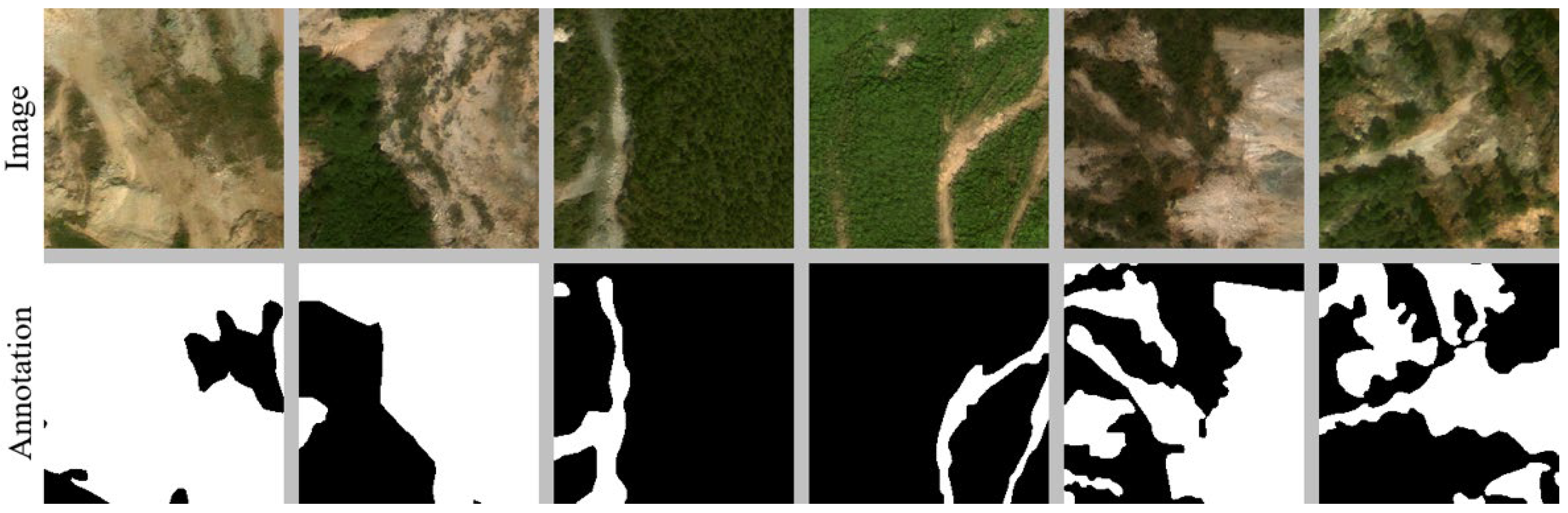
This study selected images of the 2008 Wenchuan earthquake in China, sourced from the LMHLD dataset [27], as experimental data. This dataset integrates remote sensing imagery from seven typical landslide-prone regions worldwide. In Rio de Janeiro, 716 rainfall-triggered landslides were labeled using RapidEye imagery acquired in August 2011. As a 5 m optical multispectral satellite, RapidEye supports rapid wide-area imaging and is suitable for regional-scale landslide surveys. In the Hokkaido area, 5666 landslides triggered by the 2018 earthquake were labeled using 3 m PlanetScope imagery. Benefiting from high-temporal-frequency continuous observation, PlanetScope can capture short-term surface changes after landslide occurrence. In Emilia–Romagna and Gorkha, 5847 rainfall-induced landslides and 1760 earthquake-triggered landslides were labeled using 10 m Sentinel-2 imagery acquired in August 2023 and December 2015, respectively. Sentinel-2 provides abundant spectral bands with open, free access and extensive spatial coverage, making it appropriate for preliminary large-area landslide investigation, although it lacks the capability to resolve fine features of tiny landslides. In Jiuzhaigou, 3443 landslides induced by the 2017 earthquake were labeled using 1 m Gaofen-2 imagery, which enables clear identification of the morphology and boundaries of small and medium-sized landslides. For the Wenchuan subset, 4260 coseismic landslides triggered by the 2008 Wenchuan Earthquake were labeled using 0.8 m IKONOS imagery, which is organized into 2603 image patches of 224 × 224 pixels. This imagery can finely reconstruct landslide microtopography, slide boundaries, and fractured surface characteristics (Figure 1).

The 2008 Wenchuan earthquake occurred on the Longmenshan Fault zone, located in the transitional zone between the Qinghai–Tibet Plateau and the Sichuan Basin [28]. This region is characterized by steep terrain and typical alpine canyon landforms, with ridge elevations generally ranging from 4000 to 5500 m. The earthquake triggered at least 197,481 landslides, with a total landslide area of approximately 1160 km², distributed over an area of about 110,000 km² [29]. The landslides are primarily concentrated at elevations between 1200 and 3000 m, with slope gradients ranging from 30° to 44°. The most susceptible slope aspects are east, southeast, and south, which are closely related to the dominant direction of seismic wave propagation [30]. These landslides and their secondary disasters caused approximately 15,000 deaths and disappearances and formed dozens of barrier lakes, including Tangjiashan, posing a serious threat to the safety of millions of people downstream [31].

To enhance model generalization and robustness, this study adopts an online data augmentation strategy during the training phase to increase the diversity of samples. First, the 224 × 224 input images are randomly scaled within a range of 0.75 to 1.25 times to prevent the model from overfitting to fixed-size landslide features. During random cropping, the pixel proportion of any single class does not exceed 95%, ensuring that each training iteration contains a sufficient number of valid landslide samples, given that landslide pixels account for only 32.39% of the dataset. Additionally, random horizontal flipping is applied with a 50% probability to reduce the model’s reliance on landslide orientation, and random rotation within ±10° (with zero padding for empty areas) is applied with the same probability to account for slight angular deviations in satellite image acquisition without introducing excessive deformation. Furthermore, to reduce the model’s over-reliance on fixed lighting conditions, random combinations of brightness (offset ±16), contrast and saturation (scaling within 0.8–1.2 times), and hue (offset ±9°) are applied to simulate real-world illumination variations, such as low illumination on overcast days, high contrast on sunny days, and backlit underexposed scenes.

2.2. Pixel-Level Uncertainty Analysis

Deep learning models have achieved excellent performance in tasks such as image recognition and semantic segmentation, but they cannot express the confidence level of their own predictions. This poses a serious risk in safety-critical fields such as autonomous driving, medical diagnosis, and remote sensing monitoring, where models may make erroneous predictions with extremely high confidence. Bayesian neural networks treat weights as distributions rather than fixed values and make predictions by marginalizing the posterior distribution of the weights, providing a theoretical framework to address this problem [26]. However, accurately computing this integral for deep networks with millions of parameters is computationally infeasible. In this context, Monte Carlo Dropout (MC Dropout) was proposed precisely as an efficient approximate Bayesian inference method.

MC Dropout is built upon a reinterpretation of the Dropout strategy. Dropout was originally introduced by the literature [32] as a regularization technique: during training, neuron outputs are randomly set to zero with a certain probability, forcing the network to learn redundant representations and thus mitigating overfitting. Gal and Ghahramani [21] reinterpreted Dropout at inference time (test time) as a variational approximation to the Bayesian posterior. Specifically, the objective function of training with Dropout can be formalized as a Monte Carlo approximation to the Evidence Lower Bound (ELBO) in Variational Inference, making Dropout mathematically equivalent to approximate Bayesian inference in deep Gaussian processes. This theoretical breakthrough endows Dropout with a rigorous foundation for uncertainty quantification.

Because MC Dropout requires no modification to the original network architecture and no retraining, it can be directly applied to any model that already contains Dropout layers while reusing pre-trained model weights with controllable computational overhead [33]. MC Dropout is one of the most practical uncertainty quantification methods for large-scale remote sensing image analysis where retraining is difficult or obtaining statistical priors is infeasible. The MC Dropout procedure consists of the following steps:

Step 1: Model Training

Train a deep learning model that incorporates Dropout layers (e.g., after convolutional or fully connected layers) using the standard training protocol. During this phase, Dropout acts as a regularization technique to prevent overfitting.

Step 2: Inference with Dropout Activated

Switch the trained model to inference mode but keep the Dropout layers active (in contrast to standard inference, where Dropout is disabled).

Step 3: Multiple Stochastic Forward Passes

Perform $T$ forward passes on the same input image $X$. Each pass uses a different random dropout mask ${\mathsf{ϵ}}_{\mathit{t}}$~Bern(p), generating a distinct prediction ${\widehat{\mathit{y}}}_{\mathit{t}}=\mathit{f}(\mathbf{X};\mathit{\theta } {\odot \mathsf{ϵ}}_{\mathit{t}})$

Step 4: Compute Predictive Statistics

Aggregate the $T$ predictions to compute pixel-wise statistics: mean probability, variance, and predictive entropy. These statistics quantitatively characterize the uncertainty of landslide identification results from three perspectives: average tendency, dispersion degree, and information uncertainty.

The mean predicted probability can be expressed as follows:

$$\bar{p}(x)={\displaystyle \frac{1}{T}}{\sum }_{t=1}^T{p}^{(t)}\left(x\right)$$

(1)

where $x$ denotes a pixel in the image, and $p^{\left(t\right)}\left(x\right)$ represents the probability that the $t$th model output belongs to the landslide class, ranging between 0 and 1. T is the number of Monte Carlo iterations, which is determined by the trade-off between the stability of uncertainty estimation and computational efficiency. $\bar{p}\left(x\right)$ reflects the mean predicted probability of the model for a given pixel belonging to the landslide class across multiple random iterations.

In addition, this study adopts a variance to quantify the fluctuations across different iterations, as formulated below:

$$\mathrm{Var}(x)={\displaystyle \frac{1}{T}}{\sum }_{t=1}^T{\left(p^{\left(t\right)}\left(x\right)-\bar{p}\left(x\right)\right)}^2$$

(2)

A larger variance indicates that the model’s predictions for a given pixel fluctuate significantly, implying high uncertainty. A variance approaching zero indicates that the predictions are highly consistent across iterations, meaning the model’s judgment for that pixel is stable [34]. The variance can indicate the spatial locations where the model’s predictions are likely to be erroneous, providing a basis for subsequent targeted model optimization or manual verification.

Predictive entropy is a measure of information for binary classification, which is calculated based on the mean predicted probability. Entropy originates from Shannon’s information theory and serves as a core metric for quantifying the degree of disorder (uncertainty) in the probability distribution of a random variable. Entropy originates from Shannon’s information theory and serves as a core metric for quantifying the degree of disorder (uncertainty) in the probability distribution of a random variable. A higher entropy value indicates greater uncertainty in classification decisions; conversely, a lower entropy value indicates lower uncertainty [35]. The formula is as follows:

$$H\left(x\right)=-\bar{p}\left(x\right)\overline{\ln p}\left(x\right)-\left(1-\bar{p}\left(x\right)\right)\ln \left(1-\bar{p}\left(x\right)\right)$$

(3)

In binary classification, entropy reaches its maximum when $\bar{p}\left(x\right)$ is close to 0.5, indicating that the model barely has any confidence about the pixel’s classification. When $\bar{p}\left(x\right)$ approaches 0 or 1, entropy approaches 0, indicating high confidence in the identification. Unlike variance, which reflects random fluctuations in predictions, predictive entropy emphasizes the decision state of the model classification, specifically, whether the mean probability lies in the critical classification zone. Combining variance and predictive entropy could provide a comprehensive understanding of the spatial heterogeneity of uncertainty in landslide segmentation, offering quantitative evidence to improve the model and the usability of the segmentation results. For instance, the spatial overlap of high variance and high entropy indicates simultaneous prediction fluctuations and a critical classification state for individual pixels, implying the highest likelihood of prediction error. Conversely, high entropy but low variance implies that the model is stably ‘hesitant’, that is, the identification is ambiguous yet consistent, a situation that often occurs in transitional zones between landslide and non-landslide areas.

A critical trade-off in MC Dropout-based uncertainty estimation is governed by the sampling number $T$, which concurrently determines the statistical reliability of the predictions and the computational burden [36]. A too-small $T$ causes both the variance and predictive entropy to suffer from substantial fluctuations due to stochasticity, thus failing to faithfully reflect the model’s epistemic state regarding the current input. Conversely, increasing $T$ enhances estimation reliability, but this comes at the cost of linearly growing computational expense since every forward pass requires a complete network evaluation; such overhead renders it impractical for latency-sensitive applications like autonomous driving, robotic control, and online inference. Combining the recommended values from relevant studies [21] and observing the convergence curves of the variance and predictive entropy (as shown in Figure S1), this study considers that $T=20$ is sufficiently large to maintain the reliability of the uncertainty estimation while simultaneously ensuring high computational efficiency.

2.3. Impacts of Scale Weight

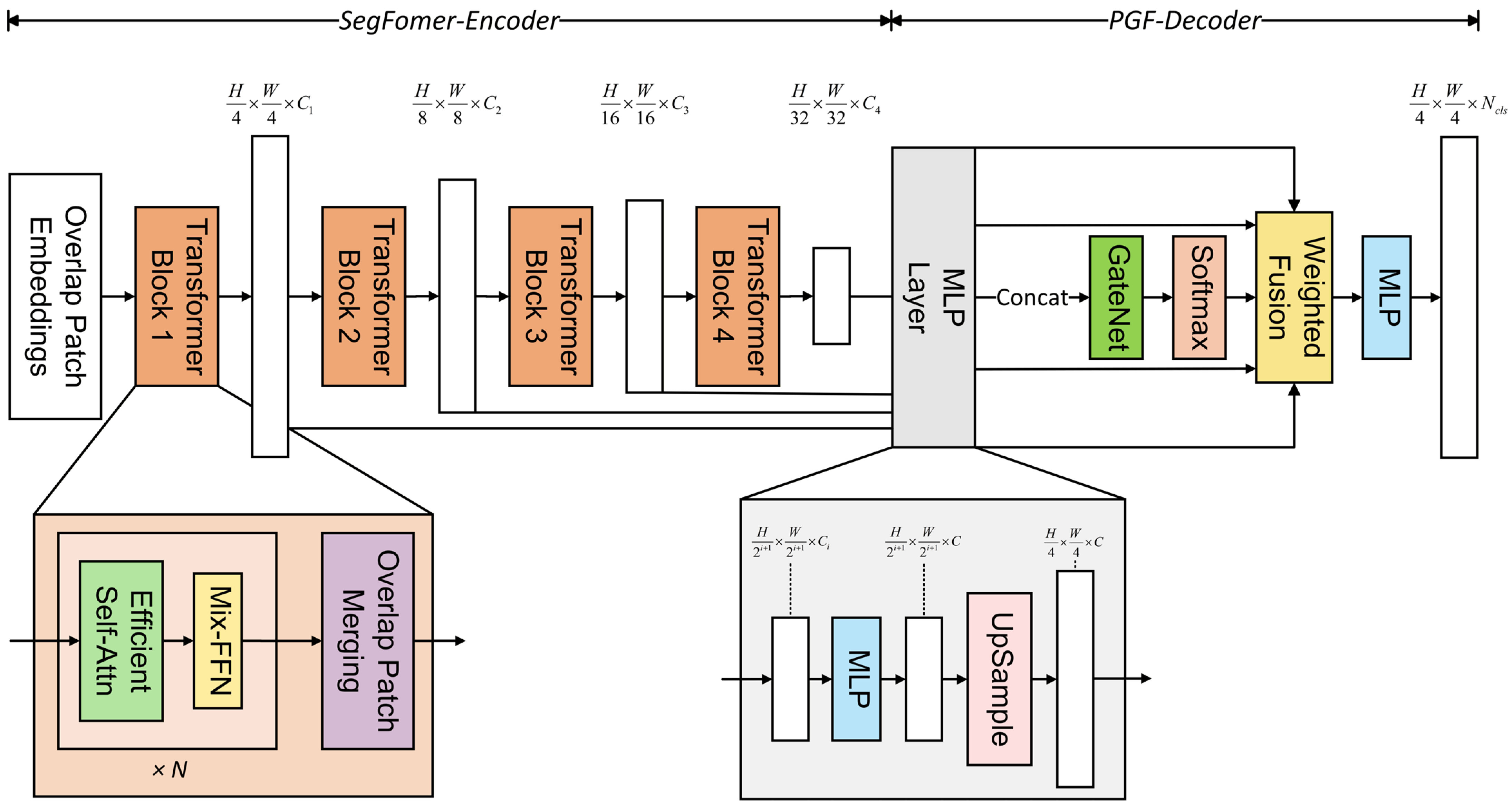
Beyond external factors, a model’s internal structure or parameters also shape the spatial distribution pattern of uncertainty [17]. As an example, this study quantifies the influence of scale weight allocation strategies on pixel-level uncertainty. To this end, this paper proposes the PGF-SegFormer model to illustrate the role of scale, which consists of a SegFormer encoder and a PGF decoder (Figure 2). The encoder is used to extract multi-level features, while in the decoding phase, an adaptive multi-scale fusion strategy based on pixel-wise gating is introduced [37]. This strategy explicitly outputs, in the form of learnable weights, the contributions of different scale weights to the final prediction, incorporates them into the fusion process, and finally produces landslide segmentation results.

The SegFormer encoder consists of four main components: overlapped patch merging, hierarchical feature representation, efficient self-attention, and Mix-FFN. Among these, overlapped patch merging partitions the input image into overlapping patches to preserve local continuity. Hierarchical feature representation gradually reduces spatial resolution while increasing channel dimensions across four stages, thereby outputting four levels of multi-scale feature maps—shallow features retain high-resolution spatial details, while deep features provide low-resolution global semantic information. Efficient self-attention reduces the sequence length before attention computation to lower computational complexity. Mix-FFN replaces the standard feedforward network with a 3 × 3 depthwise separable convolution, thereby implicitly encoding positional information without relying on explicit position encodings.

The Pixel-wise Gated Fusion (PGF) decoder first receives the four-layer features from the encoder and performs channel and spatial alignment to ensure compatibility across scales. This process involves mapping features of varying resolutions to a unified channel dimension and upsampling them to a consistent spatial scale, thereby facilitating subsequent fusion operations. Then, the PGF module jointly models the four-layer features, generates cross-scale adaptive weights for each pixel through a gating branch, and performs weighted fusion based on these weights, ultimately achieving dynamic allocation of multi-scale information contributions. Since the weights are generated at each pixel, PGF-Decoder can more precisely enhance effective scale information and reduce the influence of interfering scales in scenarios such as landslide boundaries, fine textures, and regions where landslides are easily confused with similar land covers (e.g., bare land), thereby improving prediction stability. After the PGF module completes the gated weighted fusion, the decoder sends the fused features to the prediction head to generate the final pixel-wise classification results. At the same time, the gating weights output by the PGF module serve as explicit scale contribution maps, reflecting the weight allocation of features from different scales at each pixel. Based on this scale contribution information, a data foundation can be established for subsequent correlation analysis between scale and weight allocation and the uncertainty distribution of the model.

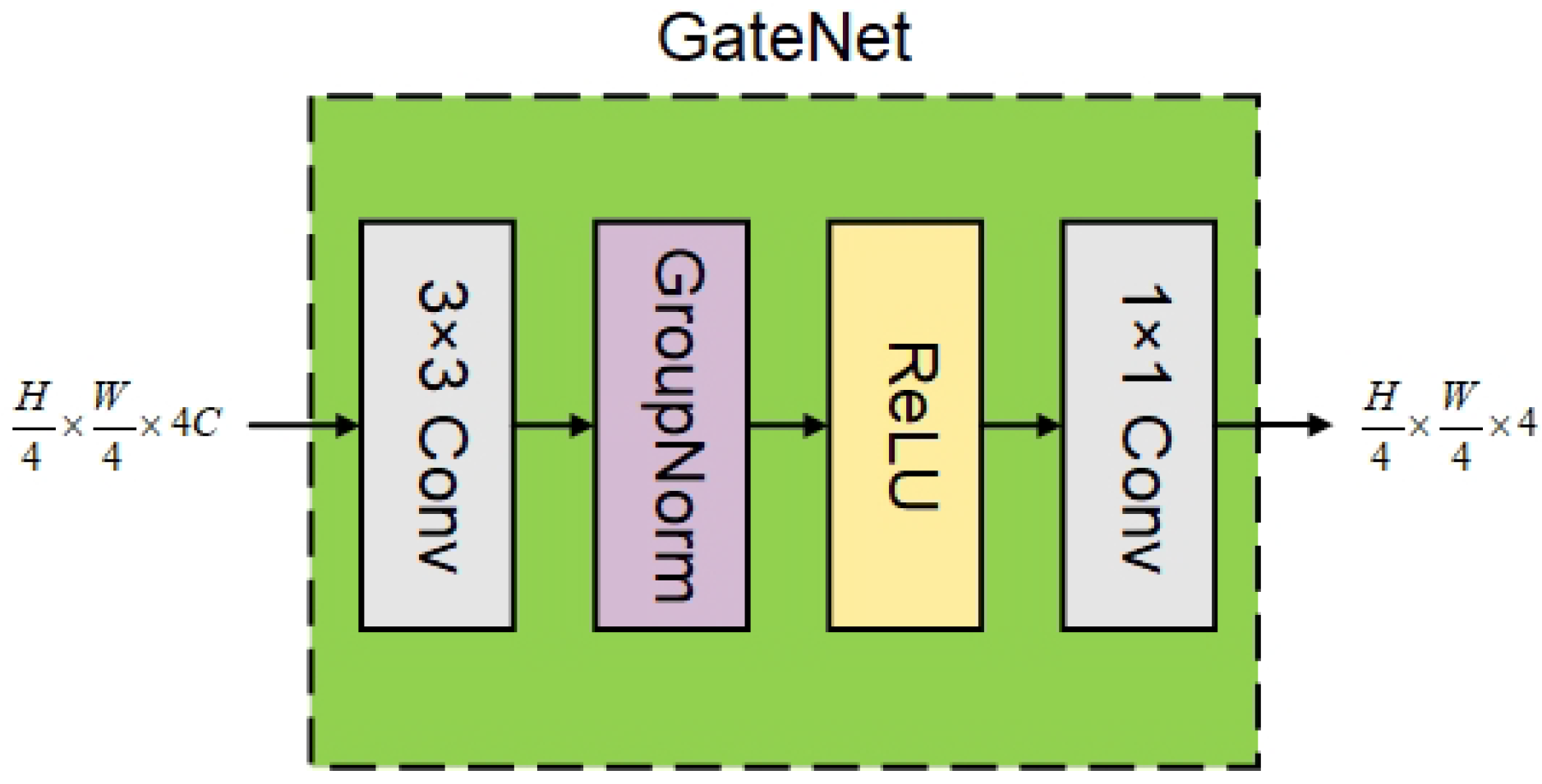
The GateNet in the decoder upsamples the feature maps from the four encoder stages to the same resolution (H/4 × W/4) and then concatenates them (Figure 3). Through convolution and SoftMax operations on the concatenated features, it generates four normalized scale weights for each pixel, reflecting the respective contributions of the four encoder output stages. The sum of the four scale weights for every pixel equals 1. The higher the weight of a given scale, the greater the contribution of its features to the prediction of that pixel. Subsequently, the model can determine whether pixel-wise uncertainty is affected by the scale weights, supporting dynamic adjustment of its feature fusion strategy, thereby reducing uncertainty and improving identification accuracy.

Considering that pixel-by-pixel analysis is computationally intensive and lacks semantic meaning, this study divides the pixels in the study area into four semantic regions. This allows for targeted analysis of uncertainty in specific landslide subregions, thereby yielding more practically valuable results. Within TP pixel clusters, pixels with a Euclidean distance greater than 2 pixels from the cluster boundary are classified as landslide interior, whereas pixels within 2 pixels of the boundary are classified as landslide border. If a TP cluster contains fewer than 50 pixels, it is considered a small landslide, and no distinction is made between interior and border regions. FP pixel clusters are defined as confused background. For each subregion, we then use the Pearson correlation coefficients between the four scale weights and the uncertainty metrics (predictive entropy and predictive variance) to evaluate the influence of scale weights on pixel-level uncertainty.

In this study, the hierarchical features extracted by the model’s backbone network are classified into four scales, which correspond to the progressively expanding receptive fields achieved through downsampling. Specifically, Scale 1 represents a shallow layer with the smallest receptive field, corresponding to the early convolutional layers of the network, which primarily extracts fine-grained pixel-level local details, such as textures, edges, and spectral information, with almost no large-scale contextual information. Scale 2 is a medium-shallow layer with a moderately expanded receptive field after one downsampling operation, capturing combined features within small local neighborhoods. Scale 3 is a medium-deep layer with a larger receptive field after further downsampling, enabling the capture of medium-range contextual semantics such as slopes and local land parcels. Scale 4 is a deep layer with the largest receptive field, located at the deepest stage of the network, which learns large-scale geomorphic features and global contextual semantics, while inevitably losing a significant amount of fine-grained detail.

2.4. PUA-Based Optimization Strategy

The landslide produced by an identification model are often directly used for disaster mapping, risk alerting, and field verification. If the results contain a large number of false detections, this not only incurs unnecessary on-site investigation costs but may also seriously affect the effectiveness of emergency response and decision-making. Considering this, if we can identify which of the marked regions are more likely to be unreliable, we can effectively mitigate the negative impact of false alarms. In order to reduce FPs, we propose a ranking-based rejection strategy. Namely, under a given rejection rate constraint, the system removes predictions with the highest risk scores, i.e., the most unreliable ones, from the output set, in exchange for a lower output error rate, ultimately achieving quantifiable and controllable decision-making risks [38,39].

Let pixels identified as landslides be denoted as ${\mathcal{S}}_P=\{x\mid \widehat{y}(x)=1\}$, where $x$ is a pixel and $\widehat{y}\left(x\right)$ is the landslide identification function. For each pixel $x\in {\mathcal{S}}_P$, an uncertainty score $s\left(x\right)$ is assigned, based on measures such as predictive entropy or sampling variance. All pixels in ${\mathcal{S}}_P$ are then sorted in descending order according to their uncertainty scores. Given a rejection rate $r\in [0,1]$, the top $r$ highest-uncertainty pixels are removed from the sorted list. Let the remaining set be $S_P^r$. The error rate $\mathrm{risk}\left(r\right)$ of $S_P^r$ is then computed as follows:

$$\mathrm{risk}(r)={\displaystyle \frac{1}{\left|S_P^r\right|}}{\sum }_{x\in S_P^r}\mathbb{I}\left(\widehat{y}\left(x\right)\ne y\left(x\right)\right)$$

(4)

where $\mathbb{I}(\cdot )$ is the indicator function, which takes the value 1 if the condition in parentheses holds, and 0 otherwise; $\left|S_P^r\right|$ denotes the total number of pixels in the retained set $S_P^r$; and $\mathrm{risk}\left(r\right)$ represents the proportion of incorrectly predicted pixels among the retained pixels, varying with the rejection rate $r$.

On the other hand, pixel-by-pixel checking of FN pixels within the background is also costly and infeasible, as the background often accounts for most of a study area. Therefore, how to efficiently prioritize the locations most likely to be FN pixels is a practical demand. In the study, we propose a ranking-based strategy to rapidly capture FN pixels. Specifically, within the set of pixels identified as background by the model, $S_N=\{x\mid \widehat{y}(x)=0\}$, entropy or variance is used as a metric to sort the pixels in descending order of uncertainty. Then, the top % of background pixels with the highest uncertainty are selected as the suggested verification set $S_N^r$. The proportion of FN pixels captured by this review set can be examined as:

$$\mathrm{F}{\mathrm{N}}_{\mathrm{capture}}(r)={\displaystyle \frac{\left|\left\{x\in S_N^r\hspace{0.33em}|\hspace{0.33em}\widehat{y}(x)=0,\hspace{0.33em}y(x)=1\right\}\right|}{\left|\left\{x\hspace{0.33em}|\hspace{0.33em}\widehat{y}(x)=0,\hspace{0.33em}y(x)=1\right\}\right|}}$$

(5)

The numerator is the number of FN pixels captured by this verification set, and the denominator is the total number of FN pixels. A higher $\mathrm{F}{\mathrm{N}}_{\mathrm{capture}}\left(r\right)$ indicates higher verification efficiency, namely, the ability to quickly find more FN pixels from a vast number of background pixels.

3. Results

3.1. The Spatial Heterogeneity of Uncertainty

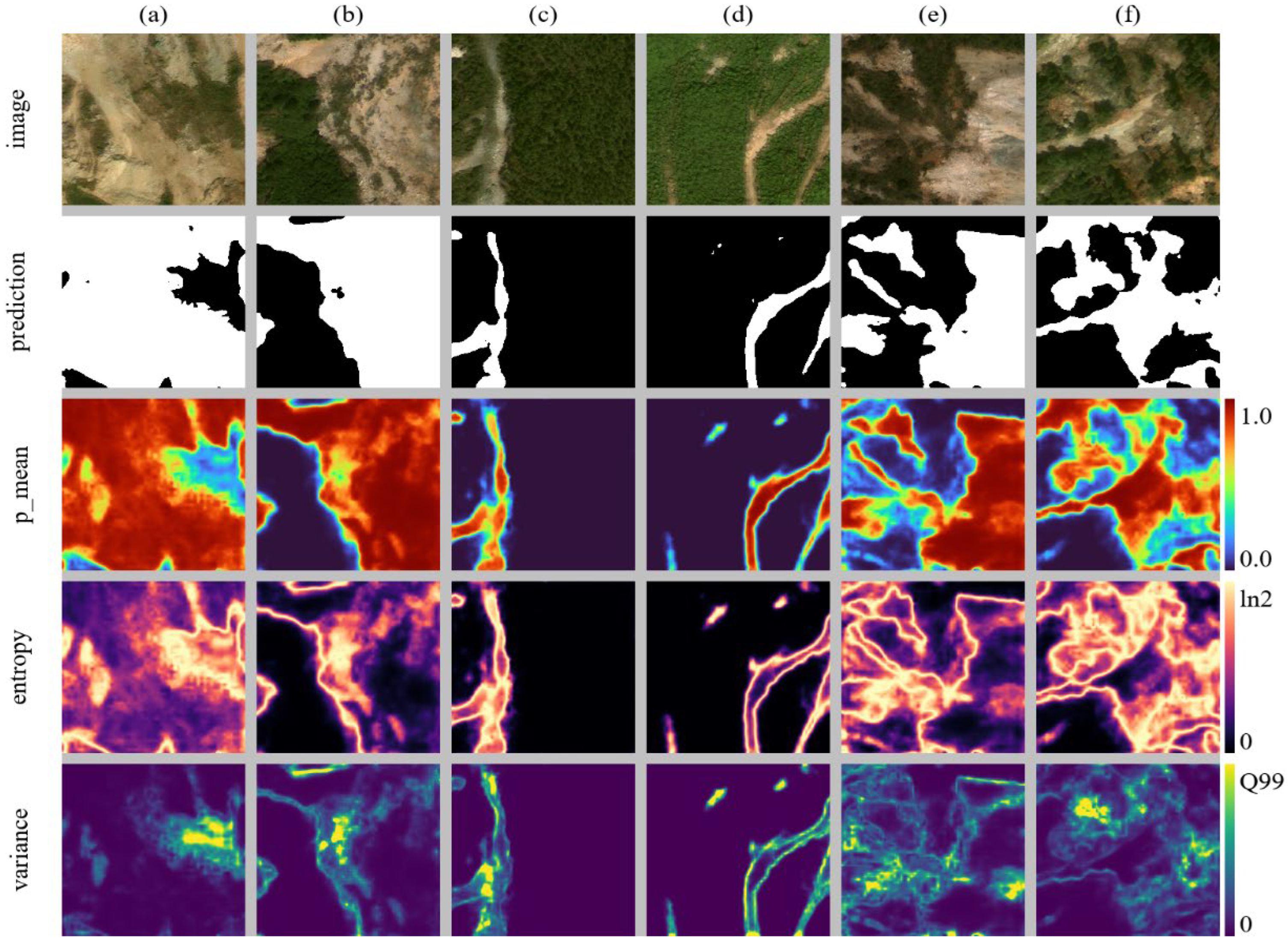
Using the MC Dropout-embedded PGF-SegFormer, we conducted pixel-wise uncertainty assessment for Wenchuan landslides. From these results, we selected six representative landslides to visually illustrate the spatial heterogeneity of uncertainty through pixel-wise mean probability maps, prediction entropy maps, and variance maps (Figure 3).

Figure 4 intuitively presents the spatial heterogeneity of landslide uncertainty. In scenes with clear landslide boundaries and typical features (Figure 4c,d), the contours of the identification results closely match the actual landslide extent. In the corresponding mean probability maps, the values within the interior of landslides are close to 1.0, suggesting high confidence. Meanwhile, the high-value areas in the entropy and variance maps are concentrated only in the narrow transition zones between landslides and the background, with extremely low values in the internal areas. This indicates that the model has high confidence in consistently identifying landslides with evident features, and uncertainty arises only from spectral mixing at the boundaries.

In Figure 4a,b,e,f, extensive mixed areas of bare soil, rock, and vegetation form a complex land surface, leading to vague landslide boundaries or unclear characteristics. The identification results exhibit serious misjudgments or boundary expansions. In the mean probability maps, not only do the actual landslide areas show high values, but also some bare soil areas with spectra similar to landslides present high-value responses. The entropy and variance maps show widespread high-value distributions, covering not only the landslide boundaries but also extending into the interior of landslides and surrounding areas. This indicates that the model has poor confidence when dealing with such scenarios, and the uncertainty exhibits significant spatial heterogeneity. The comparison between different scenarios clearly reflects the impact of land surface characteristics on uncertainty. The joint analysis of mean probability, entropy, and variance provides an intuitive basis for identifying high-uncertainty risk areas, as well as a clear direction for subsequent targeted optimization of the model’s ability to handle complex surfaces.

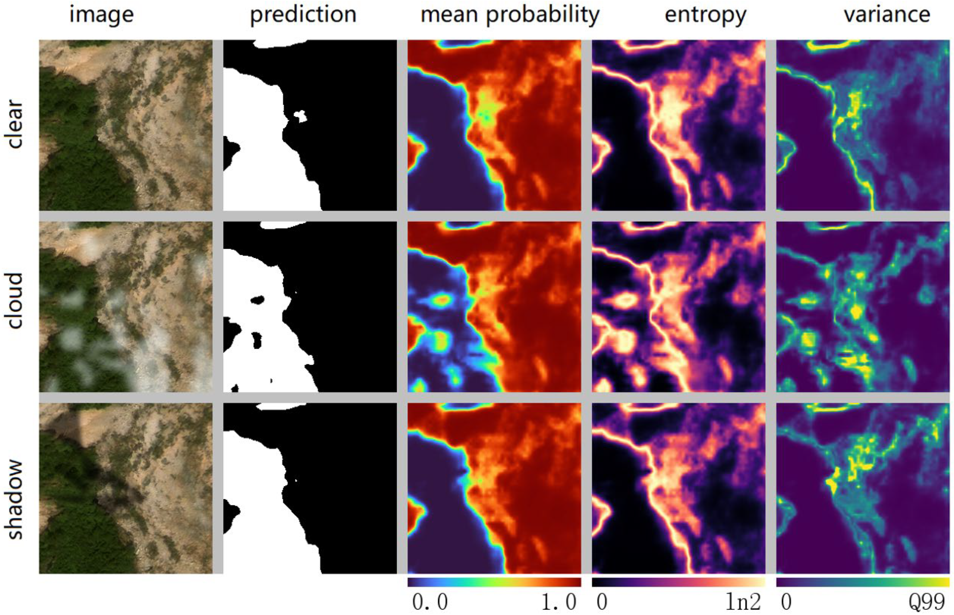
We systematically compare the variations in landslide identification results and uncertainty metrics (mean probability, entropy, and variance) under three typical scenarios, clear, cloud, and shadow, which intuitively reveal the impacts of cloud and shadow interference on model predictions. In clear scenes, the imagery is sharp and land surface characteristics are well-defined; thus, the model generates accurate landslide extents only over the actual landslide areas (Figure 5). In this scenario, the mean probability over the landslide area exhibits a gradual decrease from the interior to the boundary, while entropy and variance show localized high values only along the landslide boundary, with uncertainty within the interior remaining extremely low.

In cloud scenes, semi-transparent cloud cover interferes with the land surface spectrum, causing the model to produce additional erroneous prediction patches. Here, the mean probability over cloud-covered areas shows a pronounced high-value response, while both entropy and variance simultaneously form high-value zones in the cloud regions and along the landslide boundaries. Moreover, the uncertainty intensity in cloud areas approaches or even exceeds that of the actual landslide region, indicating that spectral interference from thin clouds leads the model to misidentify cloud areas as landslide features. Such misjudgments are accompanied by extremely low confidence and poor stability.

In shadow scenes, large dark areas formed by occlusion completely mask part of the surface information, leading to false prediction patches in shadowed areas as well. The mean probability over shadowed areas exhibits a large-area high-value distribution, while high-value zones of entropy and variance spread extensively within and along the boundaries of shadowed regions, exceeding the uncertainty level of the actual landslide area.

3.2. The Impacts of Scale Weight Allocation

First, we used the PGF decoder to disclose the weight allocation at each scale during the model’s identification process, and the statistical means are shown in

Table 1. Mean weights of the subregions at different scales.

Subregion *	Scale 1 *	Scale 2	Scale 3	Scale 4
Interior	0.714	0.257	0.014	0.016
Boundary	0.756	0.211	0.010	0.023
Small	0.779	0.194	0.007	0.020
Background	0.745	0.221	0.011	0.022

* Subregions and scales are defined in the final two paragraphs of Section 2.3.

.

Table 1 shows that the small subregion has the highest weight on Scale 1 (0.779), the lowest weight on Scale 2 (0.194), and the sum of deep features is only 2.7%, exhibiting an extreme dependence on details. This weight allocation leads the model to exhibit spurious overconfidence toward small targets, with systematically low uncertainty, while the predictions are highly sensitive to local pixel noise, edge blurring, and occlusion. Once shallow features are disturbed (e.g., shadows partially covering small targets), the model jumps from “overconfident” to completely wrong, without the uncertainty signal warning of this jump.

The boundary subregion has the second-highest weight on Scale 1 (0.756), a weight of 0.211 on Scale 2, and a deep feature sum of 3.3%. Uncertainty at boundaries is systematically low, but the actual prediction risk is high. Due to the excessively low deep weights, the model cannot utilize global semantics to confirm the class membership on both sides of the boundary, so boundary uncertainty fails to reflect true class ambiguity. In low-contrast boundaries or gradual transition zones between vegetation and soil, the model exhibits high-confidence errors. Compared with the interior subregion, the boundary subregion is forced to rely only on local gradient information, making it the most prone region for “confident errors.”

The background subregion has a weight of 0.745 on Scale 1 and 0.221 on Scale 2, with a pattern similar to that of the boundary subregion. The background usually occupies most of the image area and is highly heterogeneous, yet the model responds only with shallow features. In complex texture regions within the background (e.g., shrubs, broken rocks), the model exhibits high uncertainty, but this uncertainty is “false”—not due to class ambiguity, but because shallow features fail to match the background templates in the training set. Meanwhile, FPs in the background often correspond to low-uncertainty regions because the model is “confident” it has seen a target structure. Uncertainty within the background exhibits high-frequency spatial oscillation, lacking smooth semantic consistency.

The Interior subregion has the lowest weight on Scale 1 (0.714), the highest weight on Scale 2 (0.257), and a deep feature sum of 3.0%. Compared with other subregions, the Interior has the most contextual information, and its uncertainty is relatively the most reliable—when high uncertainty appears in the interior, it often indeed corresponds to semantic ambiguity (e.g., material composition changes within a landslide body). However, the deep weight is still less than 4%, so the model cannot use a global perspective to judge the continuity of the entire landslide body, potentially leading to unreasonable fragmented predictions within the landslide body. Both the small and interior subregions lack the global constraints of deep semantics.

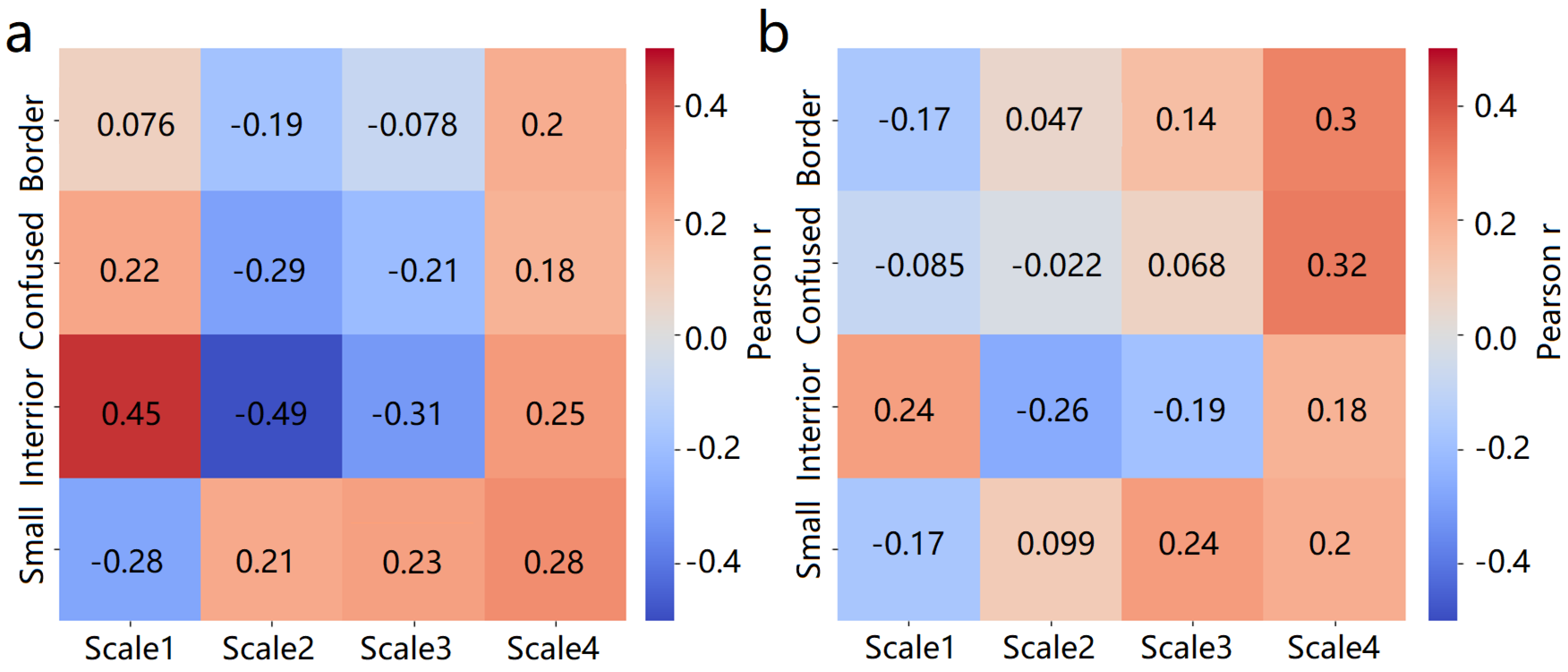
For landslide borders, Scale 1 is weakly positively correlated with entropy (0.076) and weakly negatively correlated with variance (−0.17) (Figure 6). Scale 2 shows weak correlations with entropy (−0.19) and variance (0.047), whereas Scale 4 has strong positive correlations with entropy (0.20) and variance (0.30). The corresponding weights are mainly assigned to Scale 1 (0.756) and secondarily to Scale 2 (0.211), with an extremely low weight of only 0.023 for Scale 4. The weak correlation of Scale 1 implies that high-resolution details exert limited impacts on the uncertainty of boundary identification, which conforms to the characteristic that boundary recognition highly relies on edge information. Since Scale 4 is strongly positively correlated with uncertainty but assigned a low weight, the model effectively prevents large-scale contextual information from interfering with boundary localization and restrains the growth of uncertainty in boundary areas.

In small landslide regions, Scale 1 is negatively correlated with entropy (−0.28) and variance (−0.17), while Scale 2 to Scale 4 show positive correlations with entropy (0.21, 0.23, and 0.28) and variance (0.099, 0.24, and 0.20), with the strongest correlation observed at Scale 4. Weights are highly concentrated on Scale 1 (0.779), followed by Scale 2 (0.194), and Scale 3 and Scale 4 are assigned negligible weights. The negative correlation between Scale 1 and uncertainty suggests that high-resolution details are critical for identifying small landslides, and higher weights for this scale can effectively reduce uncertainty. Given the positive correlations of Scale 2 to Scale 4 with uncertainty, the model lowers their weights to avoid the drowning effect of large-scale contextual information on small targets, thereby mitigating the prediction uncertainty for small landslides.

For the background area, Scale 1 shows weak correlations with entropy (0.22) and variance (−0.085), and Scale 2 also has weak correlations with entropy (−0.29) and variance (−0.022). By comparison, Scale 4 is significantly positively correlated with entropy (0.18) and variance (0.30). The weights are primarily distributed to Scale 1 (0.745) and Scale 2 (0.221), and Scale 4 has a low weight of 0.022. The weak correlations of Scale 1 and Scale 2 indicate that medium-scale information barely affects the uncertainty of background recognition. The low weight assigned to Scale 4, which is strongly positively correlated with uncertainty, prevents large-scale contextual features from misclassifying background areas as landslides and reduces the false prediction uncertainty of the background.

It can be observed that further optimizations can still be carried out to reduce pixel-level uncertainty. First, the differentiated contributions of Scale 3 and Scale 4 should be moderately activated. Specifically, the weights of medium and coarse scales should be slightly increased for pixels inside landslides and in the background, while the existing extremely low coarse-scale weights for boundary and small landslide pixels are retained. This allows global contextual information to constrain patches with high predictive entropy within landslides. Second, uncertainty loss feedback should be introduced to adjust scale weights. During training, pixel-wise entropy and variance are adopted to revise the real-time weights of each scale, alleviating the drawback that static average weights fail to adapt to local abnormal pixels, thereby reducing the uncertainty at landslide edges and for small landslides.

3.3. PUA-Based Improvement

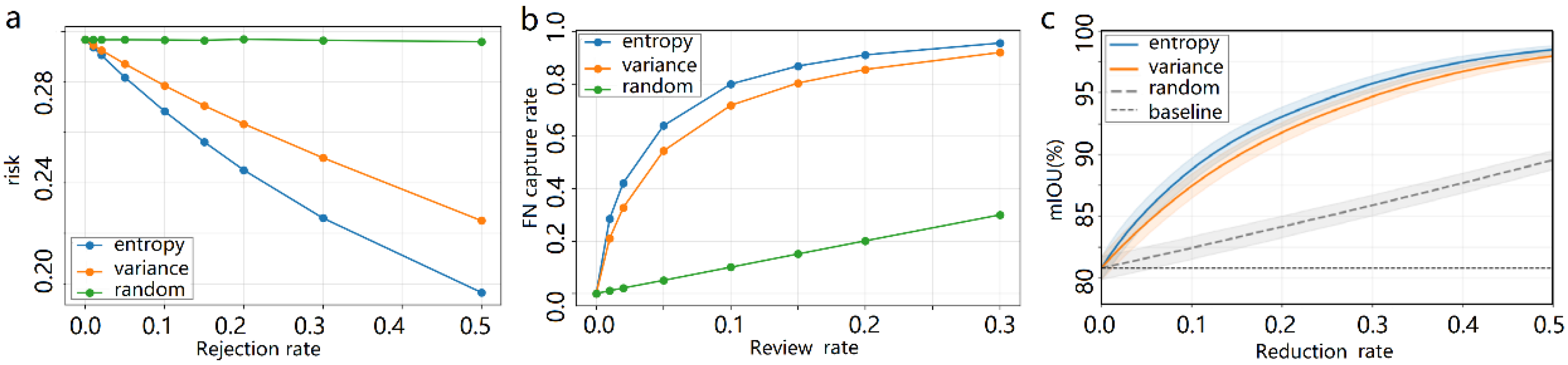
In order to obtain an effective uncertainty risk reduction approach, we compare the pixel-level error rate Risk(r) (Equation (4)) under ranking-based (using entropy or variance) and random strategies across different rejection rates (Figure 7a). At the same time, we compare the FN capture rate under different review rates using ranking-based and random strategies (Figure 7b), as well as the mIoU improvement under different reduction rates (Figure 7c).

Figure 7a demonstrates that the random rejection curve remains nearly horizontal with only minor fluctuations across the entire rejection rate range, indicating that random pixel elimination cannot fundamentally enhance the reliability of landslide identification results. In comparison, the uncertainty-driven rejection curves based on entropy and variance show a steady and substantial decline in prediction risk as the rejection rate rises, consistently lying below the random rejection baseline. Specifically, at a rejection rate of 0.2, the risk value of random rejection remains stable at 0.30, whereas variance-based uncertainty rejection reduces the risk to approximately 0.26, and entropy-based rejection further decreases it to 0.245. As the rejection rate increases to 0.3, the risk of entropy-guided rejection declines to 0.228, while variance-guided rejection drops to 0.25. When the rejection rate reaches 0.5, entropy-based and variance-based strategies reduce the prediction risk to 0.20 and 0.225, corresponding to risk reductions of approximately 33% and 25% relative to random rejection, respectively. These quantitative results validate the effectiveness of the proposed uncertainty ranking strategy. High-uncertainty pixels predominantly correspond to misclassified samples; therefore, preferentially eliminating these unreliable pixels can effectively filter classification errors and substantially improve the overall reliability of the remaining model predictions. Although the two-uncertainty metrics yield similar curve trends, entropy delivers marginally better risk control performance than variance across all rejection rates, and this superiority becomes more pronounced as the rejection rate increases. Such discrepancy arises from the different uncertainty dimensions captured by the two indicators. Entropy characterizes the overall uncertainty of model predictive distributions, while variance quantifies probability fluctuations across MC Dropout sampling iterations. This distinction results in subtle differences in their responses to typical landslide features, including ambiguous boundaries and heterogeneous surface textures. For landslide identification tasks, eliminating high-risk pixels according to uncertainty ranking can remarkably lower false detection risks, with only a tolerable reduction in spatial coverage.

Figure 7b shows that the capture rate of random review increases linearly with the review ratio, whereas uncertainty-guided review strategies substantially outperform random inspection across all review proportions. At low review ratios, both entropy-based and variance-based uncertainty ranking can efficiently capture a large proportion of missed detections, demonstrating that omission errors are highly concentrated in high-uncertainty background pixels. Specifically, at a review ratio of 5%, random review captures merely 5% of all missed detections. In contrast, entropy-based ranking captures more than 40% of omission errors, and variance-based ranking achieves over 30%. The capture rate continuously rises as the review ratio increases. At a 20% review ratio, both uncertainty-based strategies cover more than 80% of missed detection areas. When the review ratio reaches 50%, the two metrics capture nearly 90% of omission errors, while random review only achieves approximately 50%. Overall, entropy and variance exhibit comparable performance in capturing missed detections. Nevertheless, entropy yields a slightly higher capture rate at low review ratios, suggesting that it is more sensitive to the spatial distribution of omission errors. These results demonstrate that uncertainty assessment provides an effective priority scheme for background region inspection. This strategy enables limited manual verification resources to focus on high-risk areas with potential missed landslides, thereby significantly improving the overall detection efficiency.

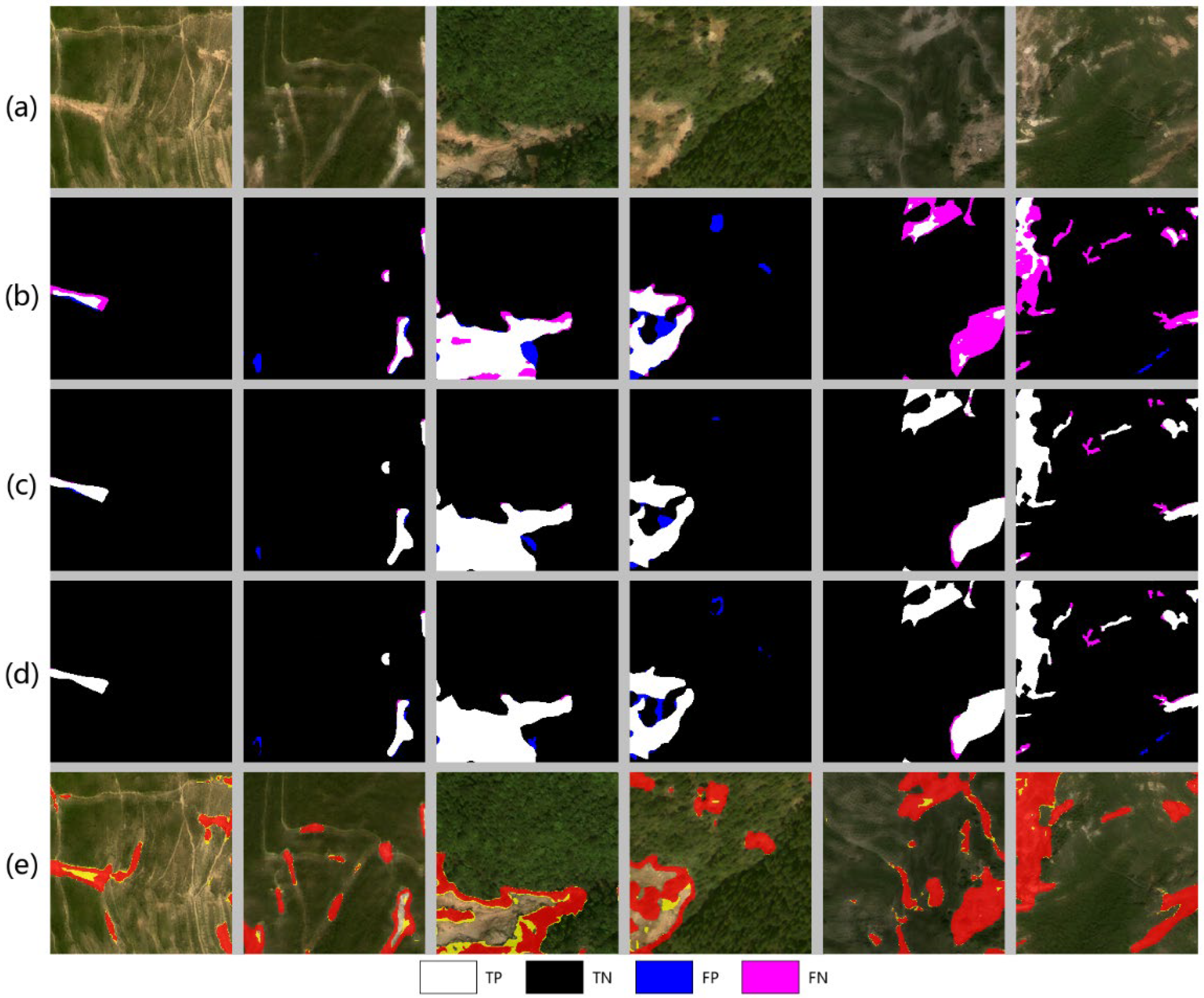
Figure 7c illustrates that the mIoU improvement achieved by the pixel recheck (removal) strategy guided by uncertainty ranking (entropy and variance) is significantly better than that of the random removal strategy. When only 10% of the pixels in the entire image are removed, the mIoU of the entropy-based strategy and the variance-based strategy rises to approximately 88.8% and 87.5%, respectively, while that of the random strategy only increases to around 82.5%. When 20% of the pixels are removed, the mIoU of the entropy-based strategy and the variance-based strategy rises to about 93.1% and 91.8%, respectively, whereas the random strategy only reaches 84.1%. This once again confirms that prioritizing the recheck (removal) of high-uncertainty pixels can efficiently improve accuracy and reliability under limited manual input. Overall, the entropy strategy achieves a higher mIoU than the variance strategy, with the largest gap occurring in the 10–20% range. This is because high-entropy pixels more completely cover the missed detection areas (Figure 8e).

Figure 8b illustrates that the initial landslide identification contains obvious FNs (blue pixels) and FPs (magenta pixels). FNs mainly occur along landslide boundaries, tiny branches, and vegetation-covered areas, while FPs are concentrated in regions with similar color and texture to landslides, such as bare land, deposits, and mountain shadows. Figure 8c,d show that uncertainty ranking-guided strategies (e.g., using entropy and variance) can effectively reduce FN and FP pixels while preserving TP and TN pixels. The entropy-based method achieves better performance in removing isolated FN regions, whereas the variance-based method works superiorly in identifying FPs connected to the main landslide bodies. Both methods perform well, although they miss some FN pixels in narrow, small landslides and partial boundaries of large landslides. Figure 8e presents the spatial distribution of high-uncertainty pixels defined by entropy and variance. This enables rapid localization of candidate pixels for manual rechecking over large areas, thereby improving working efficiency.

4. Discussion

4.1. Applicability of MC Dropout

A range of pixel-level uncertainty estimation techniques have been developed, including Deep Ensembles, Variational Inference, learning-based methods, and TTA [26]. In view of the features of mountainous landslide identification, namely prevalent pre-trained models and high efficiency demands for emergency response, MC Dropout is well-suited for pixel-level uncertainty quantification. With balanced performance, usability, and computational cost, it is highly applicable to large-scale landslide monitoring and emergency mapping.

Deep Ensembles improve the calibration performance of uncertainty by training multiple independent models [22], yet they bring extremely high computational overhead for both model training and inference, which is impractical for large-scale high-resolution remote sensing image processing in mountainous landslide surveys. Variational Inference can provide rigorous Bayesian theoretical guarantees and generate reliable posterior distributions of model weights [23]. However, it dramatically increases model parameters and computational complexity, resulting in longer training time and higher memory consumption. Additionally, the mean-field independence assumption commonly adopted in this method fails to conform to the actual characteristics of deep neural networks, further limiting its approximation accuracy.

Learning-based methods realize uncertainty estimation via a single forward pass by attaching an extra variance prediction head to the output layer, delivering the highest inference efficiency [24]. Nevertheless, this approach requires structural modification of the original network and full retraining of model parameters, which conflicts with the application demands of pre-trained landslide identification models in emergency scenarios. Moreover, it mainly captures aleatoric uncertainty induced by data noise, with limited capability to model epistemic uncertainty caused by insufficient training samples. As for TTA, it requires no network adjustment or retraining and can identify uncertainty derived from input distribution shift [25]. Unfortunately, TTA only reflects fluctuations brought by data augmentation, and cannot effectively extract the epistemic uncertainty widely existing in landslide recognition due to sparse annotated samples. It also suffers from linear computational costs arising from multiple image transformations and predictions.

Compared with the above methods, MC Dropout exhibits prominent practical and deployable advantages tailored for landslide identification tasks. Firstly, most mainstream landslide segmentation models including U-Net, SegFormer, and DeepLabv3+ are embedded with Dropout layers, so MC Dropout can be applied directly without any structural revision [21]. Secondly, it enables the reuse of pre-trained model weights and eliminates the need for retraining, which greatly reduces the time and labor costs of acquiring uncertainty information during post-disaster emergency mapping [33,36]. Thirdly, in the PyTorch 2.1.0 framework, uncertainty estimation can be realized merely by keeping the Dropout layers active during inference and executing multiple forward passes. Experimental results further verify the unique applicability of MC Dropout in mountainous landslide recognition. Its estimated uncertainty is highly consistent with manually marked disputed boundary zones, and the anisotropic distribution of variance accurately reflects the model’s confusion about exact boundary locations, supporting quantitative error assessment of landslide area calculation. By setting a proper threshold for predictive entropy, the proposed method can reduce FP rates by 30–50%, effectively suppressing FNs in complex background areas such as bare land, alluvial deposits, and mountain shadows.

4.2. Contributions and Characteristics

First, in this study, the MC Dropout-based approximate Bayesian inference framework is introduced to implement pixel-level uncertainty assessment, which effectively improves the practical applicability and interpretability of deep learning models in real-world landslide mapping scenarios. Furthermore, this paper analyzes the spatial heterogeneity of mapping uncertainty and its driving factors. The results indicate that mixed land cover (interlaced bare soil and vegetation), cloud and shadow occlusion, and abrupt terrain variation are the primary external factors inducing high model uncertainty.

Second, this study constructs the PGF-SegFormer model and reveals the adaptive regulatory strategy between multi-scale feature weight allocation and pixel-level uncertainty in landslide segmentation. Pearson correlation analysis is performed between scale weights and uncertainty indicators across four typical subregions, including landslide interiors, landslide boundaries, small landslide areas, and background areas. The analysis identifies further directions for uncertainty control, specifically: first, moderately modulating the distinct contributions from Scale 3 and Scale 4; second, employing pixel-wise entropy and variance to dynamically adjust the scale-wise weights during training.

Third, this study establishes a complete uncertainty-guided optimization framework for landslide identification. Traditional model error correction generally relies on empirical manual inspection and fixed post-processing rules, which suffers from low efficiency and non-quantifiability. Based on the quantitative ranking of entropy and variance, this study develops an FP elimination strategy and an FN priority capture strategy, which greatly improves the efficiency of model performance optimization. This study promotes landslide mapping from a single deterministic prediction paradigm to a risk-aware, reliable prediction mode, which balances prediction accuracy and operational stability well.

4.3. Implications, Limitations, and Future Work

This study offers new insights for advancing high-precision, high-reliability landslide mapping and regional risk management. First, pixel-level uncertainty quantification results can act as credible data quality labels for regional landslide inventory compilation and susceptibility evaluation. Driven by uncertainty indicators, field validation can be targeted at ambiguous areas with high prediction risks. This approach drastically reduces the workload of full-coverage field surveys and improves the update efficiency and accuracy of landslide databases in mountainous areas. Second, the uncertainty-ranking-based optimization strategy effectively mitigates the waste of emergency resources induced by FPs and prevents potential disaster risks caused by FNs. It also greatly enhances the practical value of intelligent identification results for emergency decision-making. Third, the proposed uncertainty-guided sample screening strategy provides a low-cost and high-efficiency solution for landslide dataset development. Pixels with high uncertainty correspond to the most difficult and informative samples for model training. This sample selection strategy based on uncertainty ranking facilitates the iterative optimization of training datasets. It effectively alleviates the shortage of high-quality annotated samples for remote sensing-based mountain landslide research and sustains the continuous performance improvement in subsequent models.

This study also has several limitations that need to be addressed in future research. Firstly, the experimental dataset only covers coseismic landslides in the Wenchuan earthquake-affected area, and cross-regional comparative analyses across diverse disaster types and geological environments are absent. Future research will incorporate rainfall-triggered landslides in mountainous areas of South China, loess landslides on the Loess Plateau, and engineering landslides in coastal zones to construct a multi-scenario dataset for landslide uncertainty analysis. By comparing the adaptive rules of multi-scale weights and spatial uncertainty characteristics among different landslide types, we aim to improve the generalization performance of the proposed framework.

Secondly, this study employs the classic MC Dropout method for uncertainty quantification. Despite its prominent advantages in engineering applications, this approximate Bayesian inference method tends to yield overconfident predictions in simple homogeneous regions and underconfident outputs in complex heterogeneous areas [21]. Since raw uncertainty values are not calibrated in this work, a strict quantitative correspondence between uncertainty scores and actual error probabilities has not been established, which inevitably impairs the screening accuracy of high-risk pixels to a certain degree [26]. In follow-up studies, we will adopt temperature scaling, isotonic regression, and Bayesian recalibration to calibrate the original entropy and variance derived from MC Dropout, so as to realize an accurate match between uncertainty metrics and real prediction error probabilities.

Thirdly, the coupling relationship between external environmental factors and internal multi-scale feature weights of the model has not been explored, which hinders comprehensive multi-perspective interpretation of uncertainty formation strategies. Future work will quantitatively analyze the correlations between multi-scale weight distribution and environmental factors such as vegetation coverage, slope gradient, terrain roughness, and shadow fraction. Furthermore, a geology-oriented uncertainty prediction model will be established to pre-identify high-risk recognition areas and provide prior constraints for model feature fusion.

5. Conclusions

Conventional landslide identification approaches yield deterministic classification outputs and do not account for the spatially heterogeneous uncertainty inherent in the results. In this study, we systematically examine the pixel-level spatial distribution characteristics of model prediction uncertainty, analyze its predominant controlling factors, and propose uncertainty-guided optimization strategies aimed at improving landslide identification performance. Collectively, these contributions offer meaningful insights for high-accuracy and trustworthy landslide mapping applications. In future work, we intend to incorporate a broader range of landslide types to establish a multi-scenario dataset for uncertainty analysis, thereby improving the generalization performance of the proposed framework.