Evaluating Seasonal Fidelity and Cross-Site Structural Discrimination of Sentinel-2 LAI Products in Karst Forests

Highlights

What are the main findings?

• Sentinel-2 spectral variables and LAI products tracked seasonal canopy development within individual Karst forest sites.
• Cross-site structural ranking was not consistently preserved, and the field-observed LAI range was substantially compressed, particularly in dense, vertically layered regeneration stands.

What are the implications of the main findings?

• Strong seasonal agreement between Sentinel-2-derived variables and field LAI does not necessarily imply reliable preservation of cross-site differences in forest structure.
• Sentinel-2 supports phenological monitoring and broad structural screening, but comparisons among heterogeneous stands require complementary structural information.

Abstract

Leaf area index (LAI) is widely used to characterize foliage amount and seasonal canopy development, but it captures only selected aspects of forest structure and can be difficult to retrieve reliably in heterogeneous, multilayered stands. This study evaluates Sentinel-2-based LAI information across eight sites in the Slovenian Classical Karst encompassing post-disturbance regeneration and established forest stands in dolines and relatively level inter-doline terrain. Field effective LAI measured during six periods in 2021 was compared with six Sentinel-2 spectral variables, LAI derived using the Sentinel Application Platform (SNAP), and the Copernicus Land Monitoring Service High-Resolution LAI product. The analysis explicitly distinguished two dimensions of retrieval performance that are often conflated: seasonal fidelity within sites and preservation of structural differences among sites. Most satellite-derived variables and LAI products captured the broad phenological progression from canopy development to senescence. However, strong temporal agreement within sites did not consistently translate into preservation of the ordering or magnitude of structural differences among sites. Several methods compressed the range of high effective LAI values at dense regeneration sites with substantial lower-layer vegetation. The study therefore provides a more informative framework for evaluating LAI products by identifying which component of variation drives apparent agreement. These findings indicate that Sentinel-2 can support phenological monitoring and broad screening of post-disturbance vegetation development. However, quantitative comparisons of canopy density or structural recovery across heterogeneous stands require consideration of canopy heterogeneity, potential spectral saturation, and plot-to-pixel support. The evaluation framework and the observed retrieval limitations are relevant beyond karst forests, particularly to post-disturbance stands, fragmented forests, open woodlands, and sites with dense understory or regeneration layers.

1. Introduction

Understanding how forest canopies are organized and change over time is essential for assessing ecosystem functioning, biodiversity, disturbance impacts, and recovery. Forest structure is multidimensional, encompassing canopy height, vertical layering, foliage distribution, gaps, and the spatial arrangement of vegetation. Because these attributes vary with forest-development stage, disturbance history, ecosystem type and observation scale, no single remotely sensed variable can fully provide a representation of forest structure [1]. Remote-sensing products should therefore be evaluated against the specific structural properties and monitoring purposes they are expected to support.

Leaf area index (LAI), defined as one-sided green leaf area per unit ground area, is widely used as an indicator of foliage amount and seasonal canopy development [2,3]. It is closely related to photosynthesis, transpiration, rainfall interception, energy exchange, and primary productivity [3,4]. In forests, however, LAI represents only one component of structure. Similar LAI values may arise from a closed upper canopy, a sparse overstorey above dense shrubs, or multilayered regeneration, while stands with comparable canopy height may differ substantially in foliage density. LAI should therefore be interpreted as an indicator of foliage distribution and selected aspects of forest structure rather than as a direct description of three-dimensional canopy architecture.

True LAI can be measured directly only through destructive sampling or planimetric methods. Field optical instruments such as LAI-2000 and LAI-2200 instead infer effective LAI from canopy gap fraction. These estimates assume a simplified foliage distribution and are affected by foliage clumping and the optical contribution of woody elements; where foliage and woody components cannot be separated, they are more appropriately interpreted as effective plant area. Optical methods may therefore underestimate true LAI, particularly in clumped forest canopies [2,3,5,6].

Satellite-derived LAI is conceptually distinct from field effective LAI because it is inferred from canopy reflectance through empirical, radiative-transfer, machine learning, or hybrid models. The relationship between satellite and field estimates is influenced by sensor resolution, viewing and illumination geometry, canopy structure, background reflectance, shadow, and model assumptions. The two should therefore be regarded as related but non-equivalent representations of canopy foliage, particularly in heterogeneous forests.

Sentinel-2 enables repeated LAI-related observations at spatial resolutions relevant to stand- and landscape-scale forest monitoring. Its medium-resolution multispectral bands, including several red-edge bands, support the analysis of vegetation development and canopy biochemistry [7]. LAI-related information can be derived from spectral-index relationships, empirical or machine learning models, radiative-transfer-model inversion, and hybrid approaches trained on simulated reflectance [3,8]. The Sentinel Application Platform (SNAP) Biophysical Processor implements a standard Sentinel-2 retrieval based on neural networks trained with radiative-transfer simulations, while the Copernicus Land Monitoring Service (CLMS) provides standardized LAI layers for repeated large-area monitoring [9,10]. These methods are scalable and reproducible, but they do not respond equally to canopy conditions. Spectral indices may saturate in dense vegetation, and their response is influenced by canopy structure, background reflectance, shadow, and sun-sensor geometry [11]. Model-based products depend on how well their simulated training domains represent actual leaf properties, canopy architecture, background conditions, and illumination [9,12].

Recent validation studies have demonstrated that Sentinel-2 LAI products can capture broad forest dynamics while remaining biased or insensitive under heterogeneous and high-LAI conditions. Standard retrievals have shown negative bias at moderate to high forest LAI [13], while incorporating canopy heterogeneity into radiative-transfer simulations can reduce bias but may increase retrieval variance [14]. Newer 10 m approaches improve spatial detail, yet performance remains dependent on algorithm design, canopy complexity, and reference-data quality [15,16]. Comparisons with field observations and spaceborne LiDAR similarly indicate that useful agreement at seasonal or site scales can coexist with substantial plot- and pixel-level discrepancies [17,18].

This evidence highlights a distinction that is often obscured in remote-sensing validation. A variable may show strong seasonal fidelity within sites because it follows the common progression from leaf emergence through peak development to senescence. The same variable may nevertheless poorly preserve structural differences among sites if saturation or range compression limits its ability to distinguish stands during periods of dense foliage development. Seasonal fidelity indicates whether a method tracks temporal change at a location; structural discrimination indicates whether it preserves differences in foliage density among stands observed at approximately the same time. Pooled correlations may conceal this distinction because the shared seasonal trajectory can dominate the relationship even when ecologically important cross-site contrasts are poorly represented.

Separating these two dimensions has practical value for forest monitoring and management. Products that reliably identify green-up and senescence may support phenological monitoring, disturbance detection, and broad recovery assessment. Their use for comparing regeneration density, canopy closure, or structural recovery among forest patches requires additional evidence that between-site differences are also retained. For the remote-sensing community, this distinction provides a more informative basis for assessment of performance. For forest scientists and managers, it clarifies which ecological interpretations are supported by satellite-derived LAI and when complementary observations of canopy height, gaps, or vertical layering are required.

Karst forests provide a particularly demanding setting in which to examine this problem because fine-scale variation in topography, soil development, and water availability, together with disturbance history, creates locally contrasting conditions for forest growth and vegetation structure [19,20]. Variation in slope, exposure, soil depth, and moisture can produce mosaics of established stands, canopy openings, shrub layers, and dense regeneration over short distances. Such structural heterogeneity is particularly relevant for LAI retrieval because foliage amount and vertical layering may vary substantially at spatial scales comparable to Sentinel-2 pixels. In addition, karst topography can introduce variability in illumination, shadow, background reflectance, and plot-to-pixel correspondence, further affecting optical retrievals. In the Slovenian Classical Karst, the 2014 ice storm and subsequent bark beetle outbreaks, windthrow, and salvage logging further intensified this structural heterogeneity, producing pronounced variation in canopy cover and vertical layering [21,22]. These conditions make the region a useful test environment for LAI retrieval, but the underlying challenge extends beyond karst landscapes. Similar difficulties occur in post-disturbance forests, fragmented stands, open woodlands, and forests with dense understory or regeneration layers.

This study examines how field effective LAI and Sentinel-2-derived variables represent seasonal and structural variability across eight sites in the Slovenian Classical Karst. The sites contrast regeneration areas with established forest stands and dolines with relatively level inter-doline terrain. Field effective LAI measured during six periods in 2021 is compared with six Sentinel-2 spectral variables, SNAP-derived LAI, and the Copernicus Land Monitoring Service High-Resolution LAI product. Vegetation-layer information is used to interpret the observed patterns, while comparisons among development and landform settings are treated descriptively because of the limited number of sites.

The study addresses the following research questions:

(1)

How does field effective LAI vary through the growing season and among the sampled forest-development and karst-landform settings?

(2)

To what extent do Sentinel-2 spectral variables and LAI products reproduce seasonal LAI dynamics within sites, and do methods with strong seasonal fidelity also preserve differences among structurally contrasting sites?

(3)

Under which vegetation configurations and phenological conditions do the evaluated methods compress or fail to represent high field effective LAI?

The principal contribution is a structure-oriented evaluation that separates within-site seasonal fidelity from cross-site structural discrimination. Rather than asking only whether satellite-derived variables correlate with field LAI, the analysis examines which component of variation produces that agreement. This distinction helps identify the applications for which Sentinel-2 LAI information is most reliable, the conditions under which apparently strong agreement may conceal limited structural sensitivity, and the complementary observations needed for robust forest assessment. The resulting insights are relevant to validation design, operational LAI interpretation, and the integration of optical satellite data with LiDAR, UAV, and and field observations across heterogeneous forest landscapes.

2. Materials and Methods

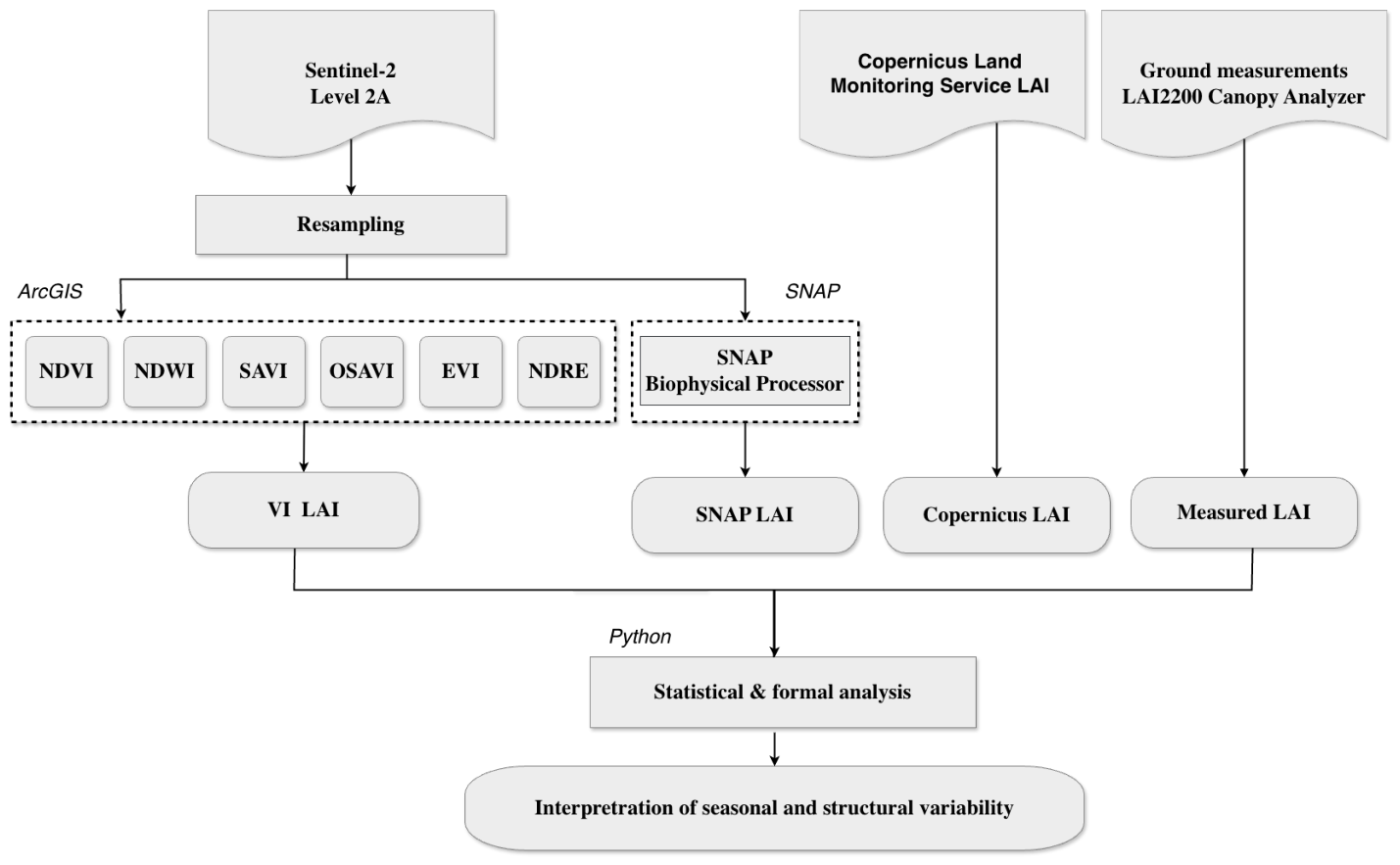
The study integrated field effective LAI observations, Sentinel-2-derived spectral variables, and LAI products to evaluate LAI representation across structurally heterogeneous karst forests (Figure 1). Eight field sites represented combinations of two forest-development conditions—regeneration areas and established forest stands—and two karst landforms—dolines and relatively level inter-doline terrain. Field effective LAI was measured during 20 campaigns in 2021, of which six campaigns with suitable temporally matched Sentinel-2 observations were retained for comparison with six Sentinel-2 spectral variables, LAI retrieved using the SNAP Biophysical Processor, and the Copernicus LAI product. Method behavior was evaluated using within-site Pearson correlations, same-date cross-site Spearman correlations, range retention, pooled linear regressions, complemented by within–between decomposition and sensitivity analyses, and exploratory Random Forest models evaluated using both apparent full-sample fit and leave-one-site-out cross-validation. Comparisons among forest-development conditions and karst landforms were interpreted descriptively.

2.1. Study Area

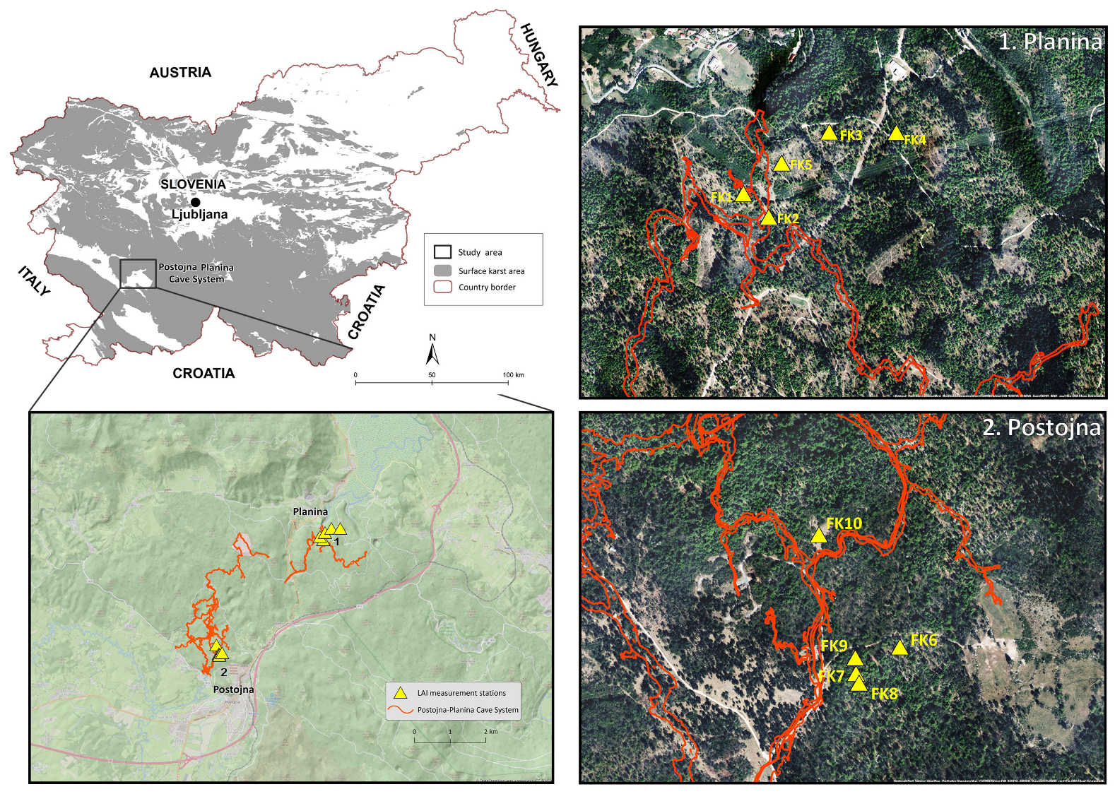
The study area is located near Postojna in the Slovenian Classical Karst, within the northwestern Dinaric Karst of southwestern Slovenia (Figure 2). It covers approximately 200 km² and includes the slopes of the Javorniki Mountains and the Planina and Postojna areas. The mean elevation is approximately 640 m a.s.l., and the terrain consists of rounded hills, slopes, relatively level inter-doline terrain, and enclosed karst depressions known as dolines [23].

Lithologically, Jurassic and Cretaceous limestones predominate [24]. Their high permeability and degree of karstification allow rapid infiltration of precipitation into the subsurface. Climatologically, the study area lies in a transition zone between Mediterranean and continental climatic influences, corresponding primarily to the Cfb and Dfb Köppen–Geiger climate classes [25]. The long-term (1981–2010) mean annual air temperature at the nearest meteorological station (Postojna 45°46′N, 14°12′E; 533 m a.s.l.) was 9.3 °C [26]. Mean monthly temperatures ranged from −0.1 °C in January to 19.0 °C in July. Mean annual precipitation was approximately 1500 mm and was relatively evenly distributed throughout the year. According to the Slovenian pedological map [27], the limestone slopes are generally characterized by rendzinas (Rendzic Leptosol), while flatter limestone surfaces are generally covered by thicker Chromic Cambisols.

The area is covered by mixed deciduous and coniferous forests that have been affected by an ice storm, bark beetle outbreaks, windthrow, and salvage logging. These disturbances created a spatial mosaic of established forest stands, canopy openings, dense regeneration, and multilayered vegetation. The area was therefore selected to represent pronounced variation in both karst microtopography and forest development. Further information on the disturbance history and its spatial distribution is provided in Supplementary Section S1.1 and Figure S1.

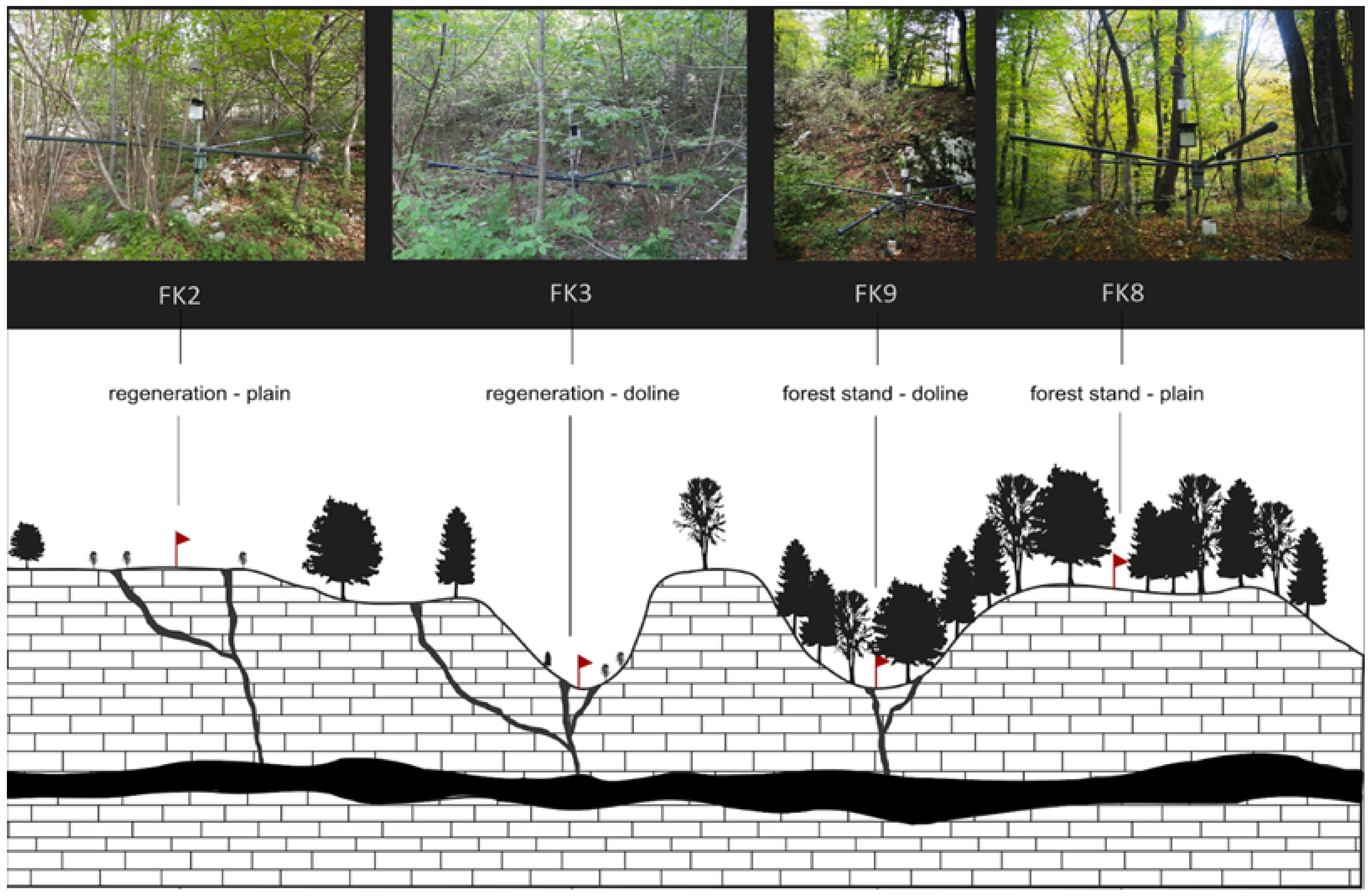
The monitoring network was selected to capture variation in karst microtopography and forest-development stage, with two sites representing each combination of established forest or regeneration and doline or relatively level inter-doline terrain. The analyzed sites were distributed between two spatial clusters, Planina (FK1–FK4) and Postojna (FK6–FK9). Pairwise distances were approximately 129–615 m within Planina and 20–108 m within Postojna, whereas distances between sites in the two clusters were approximately 4.25–4.91 km. The two clusters also differed in vegetation association (Omphalodo-Fagetum in Planina and Querco-Carpinetum in Postojna). Landform, development stage, geographic location, and vegetation composition were not fully independent, and comparisons among site groups were therefore treated as descriptive and exploratory rather than as formal tests of landform effects.

2.2. In Situ LAI Field Data

During April–November 2021, effective leaf area index (LAI) was measured in situ at eight field sites, each measuring 10 m $\times 10\mathrm{m}$ (

Table 1. In situ leaf area index (LAI) measurements from the field sites.

	Station	FK1 Forest Stand Doline	FK2 Regeneration Plain	FK3 Regeneration Doline	FK4 Forest Stand Plain	FK6 Regeneration Doline	FK7 Regeneration Plain	FK8 Forest Stand Plain	FK9 Forest Stand Doline
Field Acquisition Date
26 April 2021		0.42	–	–	–	–	–	1.00	0.71
10 May 2021		1.90	2.04	0.95	1.53	1.99	1.16	2.34	1.20
15 June 2021		4.81	10.82	7.07	2.23	5.64	4.47	5.10	2.05
13 September 2021		4.83	8.29	7.92	2.27	5.15	3.10	4.12	2.02
4 October 2021		0.34	6.08	5.97	–	5.75	3.53	4.53	1.74
11 November 2021		0.67	1.14	0.63	0.80	1.47	0.97	1.46	0.84
Mean LAI		2.16	5.67	4.51	1.71	4.00	2.65	3.09	1.43
Max LAI		4.83	10.82	7.92	2.27	5.75	4.47	5.10	2.05
St Dev		2.13	4.10	3.47	0.69	2.09	1.53	1.72	0.59

), using an LAI-2200 Plant Canopy Analyzer (LI-COR Inc., Lincoln, NE, USA). The LAI-2200 measures canopy gap fraction at five zenith angles using a fisheye optical sensor filtered to wavelengths below 490 nm, thereby maximizing the contrast between vegetation and sky [28]. A 315° field-of-view restrictor was used during all measurements. At each forest site and measurement campaign, five below-canopy readings were acquired at fixed positions above five rainfall gutters, oriented toward N, NEE, SE, SSW, and WWN. The instrument was positioned at the same locations during successive measurement campaigns to maintain a consistent spatial sampling configuration.

Above-canopy reference readings were collected in two nearby large canopy gaps, designated FK5 and FK10. These locations served only as sky-reference sites and were therefore not treated as forest sampling sites in the subsequent analysis. Effective LAI was derived by comparing the below-canopy measurements with corresponding above-canopy sky reference readings collected in these nearby open areas. Measurements were conducted under clear-sky conditions before sunrise, following the recommended protocol for measuring LAI in tall canopies and forests. These illumination conditions minimized the influence of direct solar radiation on gap-fraction measurements.

Gap-fraction measurements were processed using FV2200 software, version 2.0.0 (LI-COR Inc., Lincoln, NE, USA). The resulting estimates represent effective LAI and thus reflect the optical contribution of both foliage and woody elements within the instrument field of view. For each field site, the mean of the five LAI measurements was calculated in accordance with the LAI-2200 user manual [29] and used for analysis.

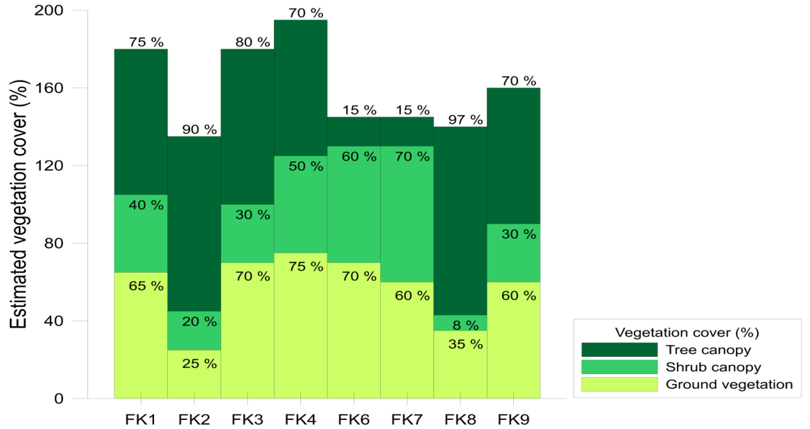
Vegetation composition and layer-specific cover were surveyed in August 2022 using the Braun–Blanquet approach. Three vertically overlapping strata were recorded: tree canopy above 5 m, shrub and lower-tree vegetation between 0.5 and 5 m, and ground vegetation below 0.5 m (Figure 3). These estimates were used to interpret differences in measured LAI and retrieval errors among regeneration areas and established forest stands. Because the vegetation survey was conducted in 2022 rather than during the 2021 LAI and satellite observations, it was used only as supplementary structural context and was not included in the quantitative analyses. Further information on sites’ biophysical and topographic parameters is provided in

Table 2. In situ LAI field sites and their biophysical and topographic parameters (top), with photographic and schematic representation of the vegetation and morphological conditions (bottom) of the different field sites.

ID	Latitude	Longitude	Location	Karst Terrain Morphology	Forest Development Phase	Vegetation Association	Slope (°)	Aspect In Situ	Orientation In Situ	Altitude (m a.s.l.)
FK1	45.81706	14.24496	Planina	doline	forest stand	Omphalodo-Fagetum	15–20	all (doline)	/	588
FK2	45.81628	14.24619	Planina	plain	regeneration	Omphalodo-Fagetum	6	330	NW	608
FK3	45.81916	14.24906	Planina	doline	regeneration	Omphalodo-Fagetum	10	265	W	565
FK4	45.81917	14.25229	Planina	plain	forest stand	Omphalodo-Fagetum	14	70	E	550
FK6	45.78757	14.21004	Postojna	doline	regeneration	Querco-Carpinetum	0–20	all (doline)	/	635
FK7	45.78692	14.20901	Postojna	plain	regeneration	Querco-Carpinetum	0	/	/	629
FK8	45.78709	14.20893	Postojna	plain	forest stand	Querco-Carpinetum	10	90, 270	E	628
FK9	45.78737	14.20891	Postojna	doline	forest stand	Querco-Carpinetum	0, 15, 30	all (doline)	/	629

.

2.3. Remote Sensing Data

Sentinel-2 is a European Space Agency (ESA) multispectral mission designed for land and vegetation monitoring. Its frequent revisit time and multispectral bands provided at spatial resolutions of 10, 20, and 60 m, including red-edge bands at 20 m resolution, support the retrieval of vegetation properties such as chlorophyll content and leaf area index (LAI) [7,30]. These characteristics are particularly useful in heterogeneous forests, where Sentinel-2 can capture small-scale canopy variability more effectively than coarser-resolution products [31] and has shown slightly better performance than Landsat 8 for forest LAI estimation [32].

Sentinel-2 Level-2A images acquired within ±1–2 days of each field campaign were accessed through Google Earth Engine using the Harmonized Sentinel-2 MSI Level-2A Surface Reflectance collection (https://developers.google.com/earth-engine/datasets/catalog/COPERNICUS_S2_SR_HARMONIZED, accessed on 17 August 2026) and used to calculate vegetation indices. No scene-level cloud-cover threshold was applied when identifying candidate acquisitions. Instead, the final image selection was based on visual inspection to confirm that pixels covering the field sites were free of clouds and cloud shadows. Because only visually confirmed cloud-free site pixels were used for extraction, no additional QA60 cloud mask or separate cloud-shadow mask was applied. Level-2A products provide orthorectified and atmospherically corrected bottom-of-atmosphere reflectance products; therefore, no additional atmospheric or aerosol correction was performed before vegetation-index calculation. Sentinel-2 spectral bands are available at native spatial resolutions of 10, 20, and 60 m. For vegetation-index calculations, all required bands were resampled to a common spatial resolution of 10 m using the nearest-neighbor method. Digital numbers were converted to surface reflectance by applying the Sentinel-2 scale factor of (${10}^{-4}$), resulting in reflectance values ranging from 0 to 1.

The corresponding original Sentinel-2 Level-2A products were downloaded from the Copernicus Data Space Ecosystem (https://dataspace.copernicus.eu/, accessed on 17 August 2026) because the ESA SNAP Biophysical Processor requires the original product structure and metadata. These products were processed in SNAP to derive Sentinel-2-based LAI estimates.

To compare the SNAP-derived LAI estimates with an operational LAI product, the corresponding Copernicus Land Monitoring Service High-Resolution LAI product was downloaded for the same acquisition dates as the Sentinel-2 imagery. The acquisition dates and product identifiers used for the spectral variables, SNAP-derived LAI, and Copernicus Land Monitoring Service High-Resolution LAI are reported in Supplementary Tables S1 and S2.

For plot-to-pixel matching, each field site was represented by a single georeferenced coordinate associated with the mean effective LAI obtained from the five fixed below-canopy measurements within the 10 m ×10 m site. The same coordinates were used for all acquisition dates and remote-sensing products. For the Sentinel-2 vegetation indices and Copernicus High-Resolution LAI, both evaluated at 10 m resolution, the single raster pixel containing the site coordinate was extracted. SNAP-derived LAI was sampled in the same way at its native 20 m resolution, thereby representing a broader spatial support than the field plot. No additional plot-area or neighborhood averaging, sub-pixel geolocation adjustment, topographic-illumination correction, or mixed-pixel weighting was applied. The associated spatial-support and geolocation uncertainties are discussed in Section 4.6.

2.4. Sentinel-2 Vegetation Indices

Six vegetation indices were calculated from Sentinel-2 surface-reflectance bands (

Table 3. Sentinel-2 vegetation indices evaluated in the study.

Index	Equation	Primary Sensitivity
NDVI	${\displaystyle \frac{{\rho }_{\mathrm{NIR}}-{\rho }_{\mathrm{R}}}{{\rho }_{\mathrm{NIR}}+{\rho }_{\mathrm{R}}}}$	Canopy greenness and photosynthetically active vegetation, with potential saturation under dense canopies [35].
NDWI	${\displaystyle \frac{{\rho }_{\mathrm{Green}}-{\rho }_{\mathrm{NIR}}}{{\rho }_{\mathrm{Green}}+{\rho }_{\mathrm{NIR}}}}$	McFeeters water index, sensitive primarily to open water and contrasts between vegetation and low-reflectance background features [36].
SAVI	${\displaystyle (1+L)\frac{{\rho }_{\mathrm{NIR}}-{\rho }_{\mathrm{R}}}{{\rho }_{\mathrm{NIR}}+{\rho }_{\mathrm{R}}+L}}$	Vegetation response adjusted for soil and background brightness [37,38].
OSAVI	${\displaystyle \frac{{\rho }_{\mathrm{NIR}}-{\rho }_{\mathrm{R}}}{{\rho }_{\mathrm{NIR}}+{\rho }_{\mathrm{R}}+0.16}}$	Vegetation response with a fixed soil-background adjustment [39].
EVI	${\displaystyle 2.5\frac{{\rho }_{\mathrm{NIR}}-{\rho }_{\mathrm{R}}}{{\rho }_{\mathrm{NIR}}+6{\rho }_{\mathrm{R}}-7.5{\rho }_{\mathrm{B}}+1}}$	Enhanced sensitivity under high biomass and reduced influence ofatmospheric and background effects [40].
NDRE	${\displaystyle \frac{{\rho }_{\mathrm{NIR}}-{\rho }_{\mathrm{RE}}}{{\rho }_{\mathrm{NIR}}+{\rho }_{\mathrm{RE}}}}$	Red-edge response associated with canopy chlorophyll and seasonal vegetation development [41,42,43].

): the normalized difference vegetation index (NDVI), normalized difference water index (NDWI), soil-adjusted vegetation index (SAVI), optimized soil-adjusted vegetation index (OSAVI), enhanced vegetation index (EVI), and normalized difference red-edge index (NDRE). These indices were selected to represent complementary sensitivities to canopy greenness, background exposure, high-biomass vegetation, and red-edge response [33,34].

Here, ${\rho }_{\mathrm{B}}$, ${\rho }_{\mathrm{Green}}$, ${\rho }_{\mathrm{R}}$, ${\rho }_{\mathrm{RE}}$, and ${\rho }_{\mathrm{NIR}}$ denote surface reflectance in the blue, green, red, red-edge, and near-infrared bands, respectively. For SAVI, the canopy-background adjustment factor was set to $L=0.428$, following the Sentinel Hub implementation of SAVI for Sentinel-2 [44].

2.5. SNAP Biophysical Processor Leaf Area Index

LAI was also retrieved using the Sentinel-2 Biophysical Processor implemented in SNAP version 9.0.0. The processor uses neural networks trained on synthetic canopy reflectance generated using radiative-transfer simulations. Inputs include eight Sentinel-2 reflectance bands (B3, B4, B5, B6, B7, B8A, B11, and B12), together with solar and observation geometry [9]. The processor uses separate neural-network parameterizations for Sentinel-2A and Sentinel-2B to account for differences in sensor spectral response, and the sensor setting was matched to the source platform for each acquisition (Table S1). SNAP has since advanced to version 13.0, in which the sensor-specific 20 m Biophysical Processor architecture is retained. The Sentinel-2 scenes were processed at 20 m, matching the native resolution of several required red-edge and shortwave-infrared bands and the eight-band network documented for the 20 m product [9].

The accompanying LAI quality-flag band was inspected for all extracted site-date values. The INPUT_OUT_OF_RANGE flag indicates that the spectral inputs fall outside the neural-network definition domain represented by the simulated training data and was therefore treated as an indicator of increased retrieval uncertainty rather than as an automatic exclusion criterion [45]. Output-thresholding and output-too-low/high flags were examined in the same way. No observations were excluded solely on the basis of these flags, because they identify retrievals requiring additional scrutiny rather than necessarily invalid values, and such exclusion would have substantially reduced the limited sample size. The occurrence and implications of the flags are examined in the sensitivity analysis and considered when interpreting the SNAP-derived LAI results.

2.6. Copernicus Land Monitoring Service High-Resolution Leaf Area Index

The Copernicus Land Monitoring Service High-Resolution Vegetation Phenology and Productivity (HR-VPP) suite provides a raw Leaf Area Index product for Europe at 10 m spatial resolution for individual Sentinel-2 acquisition dates [10]. This operational product offers another neural network-based approach to LAI estimation. The algorithm behind the Copernicus LAI product is based on a neural network trained on synthetic data generated by radiative transfer models such as PROSAIL, similar to the SNAP processor, but adapted for large-scale automated processing across Europe. The Copernicus LAI product uses eight spectral bands and incorporates temporal smoothing techniques to ensure continuity and minimize cloud-related noise. The final LAI values are delivered as part of the Copernicus Global Land and HR-VPP portfolios and are scaled by a factor of 1000 (requiring conversion before analysis). For the Copernicus High-Resolution LAI product used in this study, the QFLAG2 layer was not used as an additional exclusion criterion. Official product assessments have examined its spatial completeness, temporal consistency, and agreement with established Copernicus vegetation products across several land-cover classes [46]. Independent evaluations of the broader HR-VPP suite have also demonstrated its utility for agricultural phenology monitoring [15,32], although direct field validation of the operational 10 m LAI layer remains limited.

2.7. Statistical Analysis

The analysis combined complementary approaches to distinguish seasonal fidelity within sites from same-date cross-site structural discrimination and to assess the robustness of satellite–field relationships. These included within-site seasonal correlations, same-date cross-site rank correlations and LAI range retention, pooled linear regressions with sensitivity analyses, a within–between decomposition of repeated site observations, and exploratory Random Forest regression evaluated using both apparent full-sample fit and leave-one-site-out cross-validation. Descriptive comparisons among forest-development conditions and karst landforms were used to provide structural context.

2.7.1. Seasonal and Structural Variation

Field effective LAI was first summarized by site, measurement date, forest- development condition, and karst landform. Seasonal trajectories were compared among the four structural combinations represented in the sampling design. Because each combination contained only two sites, comparisons between regeneration areas and established forest stands or between dolines and relatively level inter-doline terrain were treated as descriptive and exploratory.

Seasonal fidelity was assessed by calculating the Pearson correlation coefficient between each remote-sensing variable and field effective LAI across the available dates within each site. Given the limited number of observations per site, the coefficients were interpreted cautiously and together with the observed seasonal trajectories, rather than as stand-alone evidence of seasonal consistency. These site-level correlations describe the extent to which a retrieval method followed seasonal leaf development and senescence at a given site.

Cross-site structural differences were evaluated descriptively using the site-date observations and, more explicitly, through same-date comparisons that assessed whether satellite-derived variables preserved the relative ordering and magnitude of field effective LAI among sites. Additional sensitivity analyses were used to examine the robustness of the observed satellite–field relationships to geographic grouping and the maximum field LAI observation.

2.7.2. Same-Date Cross-Site Relationships

To evaluate whether the satellite-derived variables also preserved differences among sites independently of the shared seasonal trajectory, Spearman rank correlations were calculated separately across sites for each measurement date. The April campaign was excluded because field effective LAI was available at only three sites. For the same-date summaries, the NDWI correlation coefficients were multiplied by $-1$ so that positive values consistently indicated agreement with increasing vegetation response. Because each date contained only seven or eight matched sites, the resulting coefficients were interpreted descriptively rather than as formal inferential tests.

Because SNAP-derived LAI and Copernicus LAI are expressed in the same nominal units as the field observations, their ability to preserve the magnitude of same-date cross-site variation was additionally assessed using percentage range retention. For product m and measurement date t, range retention was calculated as:

$${\mathrm{RR}}_{m,t}=100{\displaystyle \frac{{max}_i\left(P_{m,i,t}\right)-{min}_i\left(P_{m,i,t}\right)}{{max}_i\left(F_{i,t}\right)-{min}_i\left(F_{i,t}\right)}},$$

(1)

where $P_{m,i,t}$ is the LAI value returned by product m at site i on date t, and $F_{i,t}$ is the corresponding field effective LAI. A value of $\mathrm{RR}=100\%$ indicates that the product and field observations have the same cross-site range. Values below 100% indicate compression of the observed range, whereas values above 100% indicate that the product produced a wider cross-site range than the field observations. Range retention describes the magnitude, but not the ordering, of cross-site variation and was therefore interpreted together with the same-date Spearman correlations.

Range retention was calculated only for SNAP-derived LAI and Copernicus LAI because these products are expressed in nominal LAI units and can be compared directly with the field effective LAI range. Raw ranges of the dimensionless vegetation indices were not directly compared with field LAI. The April campaign was excluded from the same-date cross-site analyses because field observations were available at only three sites.

2.7.3. Regression and Absolute Agreement

Linear regression was used to characterize the relationship between each satellite-derived variable and field effective LAI. The coefficient of determination ($R^2$) was used to summarize linear association. For the Random Forest models, mean absolute error (MAE) and mean squared error (MSE) were used to describe apparent differences between field effective LAI and fitted model estimates in LAI units; MSE is expressed in squared LAI units.

$$\mathrm{MAE}={\displaystyle \frac{1}{n}}{\displaystyle \sum _{i=1}^n}\left|{\widehat{y}}_i-y_i\right|,$$

(2)

$$\mathrm{MSE}={\displaystyle \frac{1}{n}}{\displaystyle \sum _{i=1}^n}{\left({\widehat{y}}_i-y_i\right)}^2,$$

(3)

$$R^2=1-{\displaystyle \frac{{\sum }_{i=1}^n{\left(y_i-{\widehat{y}}_i\right)}^2}{{\sum }_{i=1}^n{\left(y_i-\overline{y}\right)}^2}},$$

(4)

where $y_i$ is the field effective LAI, ${\widehat{y}}_i$ is the corresponding estimated LAI, $\overline{y}$ is the mean field effective LAI, and n is the number of matched observations.

The robustness of the pooled relationships was additionally examined by repeating the linear regressions separately for the Planina and Postojna site groups and after excluding the single maximum field effective LAI observation (FK2, 15 June 2021; LAI = 10.82 m² m⁻²). To assess whether this maximum observation affected the same-date structural comparison during peak canopy development, the June cross-site Spearman correlations were also recalculated after its exclusion.

2.7.4. Decomposition of Within- and Between-Site Variation

To account explicitly for the repeated observations within field sites, the pooled linear relationships were complemented by a within–between decomposition. For each remote-sensing variable $X_{ij}$ and field effective LAI $Y_{ij}$, where i denotes site and j denotes measurement date, site means ${\overline{X}}_i$ and ${\overline{Y}}_i$ were calculated. The within-site association was evaluated by regressing the site-centered values $Y_{ij}-{\overline{Y}}_i$ on $X_{ij}-{\overline{X}}_i$, thereby describing temporal covariation within sites independently of persistent between-site differences. The between-site association was evaluated by regressing the eight site-mean field LAI values ${\overline{Y}}_i$ on the corresponding site-mean remote-sensing values ${\overline{X}}_i$. Within- and between-site slopes and coefficients of determination were interpreted descriptively because of the limited number of sites and measurement dates.

2.7.5. Random Forest Regression

Random Forest Regression was used as an exploratory nonlinear approach to characterize associations between satellite-derived variables and field effective LAI [47,48,49]. Separate univariate models were fitted using each vegetation index or LAI product as the predictor and field effective LAI as the response. The models used 100 trees, the squared-error split criterion, min_samples_split = 2, and min_samples_leaf = 1, selected as a standard fixed setting for this exploratory analysis. Given that the Random Forest analysis was intended to characterize nonlinear associations within the observed dataset rather than to develop an optimized predictive model, no additional hyperparameter tuning was performed.

To evaluate robustness and reduce the risk of overinterpreting apparent full-sample fit, a leave-one-site-out cross-validation procedure was also applied. In each fold, all observations from one field site were withheld as the test set, and the model was trained on observations from the remaining seven sites. Predictions from the eight held-out folds were then combined to calculate cross-validated MAE, MSE, and $R^2$. This site-blocked validation was used because the dataset contained repeated observations from the same field sites; random observation-level cross-validation would risk placing observations from the same site in both training and test sets and could therefore overestimate transferability. Apparent full-sample metrics and leave-one-site-out metrics are reported separately.

All statistical analyses were conducted in Python 3.10, using NumPy 1.24, pandas 2.0, SciPy 1.10, and scikit-learn 1.3. Vegetation-index and LAI maps were generated using ArcGIS Desktop 10.8.1 (Esri, Redlands, CA, USA) and SNAP 9.0.0.

3. Results

3.1. Seasonal LAI Variation Across Forest Structural Settings

Field effective LAI showed pronounced seasonal and spatial variation across the eight sites. Because each forest-development and karst-landform combination was represented by only two sites, the comparisons in this section are interpreted descriptively and are used to provide structural context for the satellite–field comparisons. At the beginning of leaf development in late April, the three available measurements ranged from 0.42 to 1.00 m² m^$-2$. LAI increased rapidly during spring and reached its highest values in June, when mean LAI was $3.6\pm 1.6$ m² m^$-2$ across established forest stands and $6.9\pm 2.8$ m² m^$-2$ across regeneration sites.

The structural contrast between regeneration and established forest stands was especially pronounced during full leaf development (

Table 4. Mean field effective LAI (m² m^$-2$) for the four combinations of forest-development condition and karst landform. Each value represents two sites unless measurements were unavailable.

Date	Established Forest Stand, Doline	Established Forest Stand, Relatively Level Inter-Doline Terrain	Regeneration, Doline	Regeneration, Relatively Level Inter-Doline Terrain
26 April	0.57	1.00	–	–
10 May	1.55	1.94	1.47	1.60
15 June	3.43	3.67	6.36	7.65
13 September	3.43	3.20	6.54	5.70
4 October	1.04	4.53	5.86	4.81
11 November	0.76	1.13	1.05	1.06

). In June, mean LAI was 6.36 and 7.65 m² m^$-2$ in regeneration sites located in dolines and on relatively level inter-doline terrain, respectively, compared with 3.43 and 3.67 m² m^$-2$ in the corresponding established forest stands. Regeneration sites also retained higher LAI into September and October. In this limited sample, contrasts between regeneration areas and established forest stands were descriptively larger during full leaf development than contrasts between dolines and relatively level inter-doline terrain within the same development condition. These patterns are reported as site-level descriptive contrasts rather than as statistically tested group effects.

The highest individual LAI was recorded at FK2, a regeneration site on relatively level inter-doline terrain, where LAI reached 10.82 m² m^$-2$ in June. FK3, a regeneration site in a doline, reached 7.92 m² m^$-2$ in September. Both sites contained extensive hazel (Corylus avellana) in the lower tree and shrub layers. The lowest summer maximum occurred at FK9, an established forest stand in a doline, where LAI reached only 2.05 m² m^$-2$ in June. Together with the vegetation-layer survey, these contrasts are consistent with possible contributions from lower-tree, shrub, and ground vegetation cover to the high field effective LAI at the regeneration sites; however, the available data do not quantify vertical foliage distribution. This interpretation is based on the layer-specific cover estimates and should not be read as a direct measurement of vertical foliage distribution.

3.2. Seasonal Fidelity of Sentinel-2-Based Variables

The Sentinel-2 spectral variables and both LAI products reproduced the broad phenological progression observed in the field: relatively low values before complete leaf emergence, an increase toward June, and a decline during autumn. The strength of these temporal relationships nevertheless varied among sites and retrieval methods (

Table 5. Site-level Pearson correlations between field effective LAI and the Sentinel-2-derived variables across the available measurement dates. Correlations are based on four to six observations (n) per site.

Method	FK1	FK2	FK3	FK4	FK6	FK7	FK8	FK9
NDVI	0.88	0.68	0.56	0.94	0.56	0.80	0.73	0.81
NDWI	−0.88	−0.70	−0.56	−0.94	−0.60	−0.80	−0.66	−0.72
SAVI	0.79	0.69	0.60	0.91	0.74	0.92	0.83	0.83
OSAVI	0.83	0.69	0.59	0.92	0.69	0.89	0.80	0.83
EVI	0.76	0.74	0.63	0.91	0.88	0.97	0.91	0.87
NDRE	0.95	0.77	0.74	1.00	0.68	0.85	0.82	0.86
SNAP	0.96	0.76	0.63	0.89	0.67	0.79	0.84	0.88
Copernicus	0.87	0.71	0.48	0.91	0.55	0.77	0.70	0.74
n	6	5	5	4	5	5	6	6

).

The strongest site-level relationships included NDRE at FK4 ($r=1.00$), EVI at FK7 ($r=0.97$), SNAP-derived LAI at FK1 ($r=0.96$), and NDRE at FK1 ($r=0.95$). High correlations were also observed for NDVI and NDWI at FK4 ($\left|r\right|=0.94$), while OSAVI at FK4 and SAVI at FK7 both reached $r=0.92$.

Temporal relationships were generally weaker at FK3 than at most other sites. At this heterogeneous regeneration site, correlations for the variables expected to increase with LAI ranged from $r=0.48$ for Copernicus LAI to $r=0.74$ for NDRE.

SNAP-derived LAI and EVI each reached $r=0.63$, while OSAVI reached $r=0.59$. These results suggest that the seasonal development of the multilayered vegetation at FK3 was represented less consistently than at several other sites, although the small number of observations prevents firm attribution of this pattern to vegetation structure alone.

The Copernicus Land Monitoring Service High-Resolution LAI product showed positive temporal correlations at all sites, ranging from $r=0.48$ at FK3 to $r=0.91$ at FK4. Correlations were also relatively high at FK1 ($r=0.87$), but more moderate at FK6 ($r=0.55$), FK2 ($r=0.71$), FK8 ($r=0.70$), and FK9 ($r=0.74$). The product therefore generally followed seasonal canopy development, while the strength of the relationship differed substantially among sites.

The negative coefficients obtained for NDWI reflect the inverse direction of the green–NIR formulation used in this study rather than poorer seasonal tracking. As field effective LAI increased, NDWI generally became more negative. Its seasonal fidelity should therefore be interpreted from the magnitude and direction of the coefficient; the values do not provide direct evidence of canopy moisture conditions or drought.

The complete site- and date-specific values for NDVI, NDWI, SAVI, OSAVI, EVI, NDRE, SNAP LAI, and Copernicus LAI are reported in Supplementary Tables S3–S10. A consolidated comparison of the within-site correlations is provided in Supplementary Table S11.

3.3. Pooled Relationships and Cross-Site Structural Discrimination

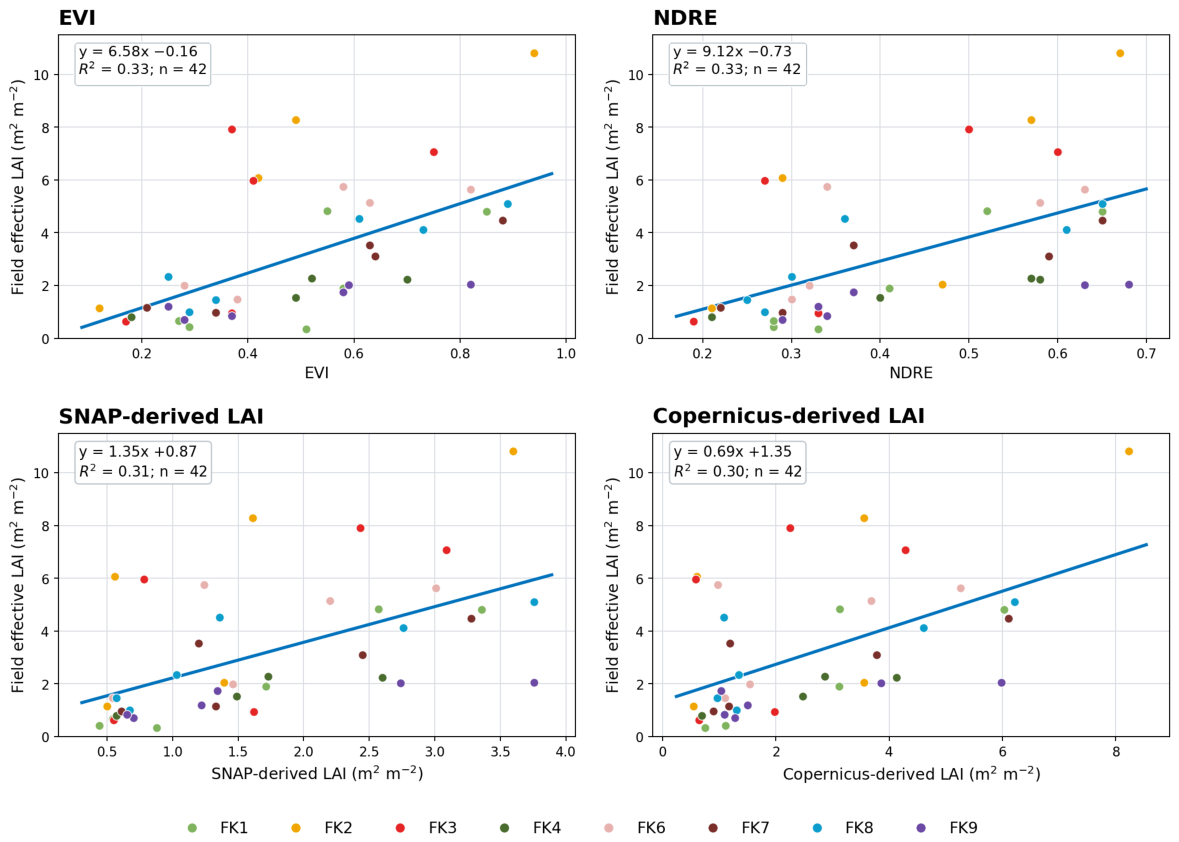
The pooled regressions explained a modest proportion of the combined cross-site and cross-date variability (Figure 4). Among the selected relationships, $R^2$ values ranged from 0.30 for Copernicus LAI, 0.31 for SNAP-derived LAI, and 0.33 for both NDRE and EVI. These pooled associations were considerably weaker than many of the within-site temporal correlations reported in Table 5. Cross-site ranges and percentage range-retention values for the two LAI products are summarized in

Table 6. Cross-site LAI ranges and percentage range retention for the SNAP-derived and Copernicus LAI products across field campaigns. LAI ranges are expressed in m² m^$-2$.

Date	Field LAI Range	SNAP LAI Range	SNAP Range Retention (%)	Copernicus LAI Range	Copernicus LAI Range Retention (%)
10 May	1.38	0.68	49	2.38	172
15 June	8.77	1.16	13	4.10	47
13 September	6.28	1.15	18	2.36	38
4 October	5.75	0.80	14	0.61	11
11 November	0.84	0.15	18	0.55	66

. Because these pooled regressions combine repeated observations from the same sites, the reported $R^2$ values are interpreted as descriptive measures of overall association rather than as estimates based on 42 statistically independent observations.

Same-date comparisons showed more directly that pooled agreement did not imply preservation of structural differences among sites. In June, when field effective LAI ranged from 2.05 to 10.82 m²  m^$-2$, cross-site Spearman correlations were weak, ranging from $-0.12$ for NDRE to 0.31 for EVI and Copernicus LAI. In September, all evaluated variables showed negative cross-site rank correlations, ranging from $-0.69$ for NDVI to $-0.40$ for SAVI and Copernicus LAI. The same pattern persisted in October, when coefficients ranged from $-0.57$ for NDRE to $-0.39$ for EVI. Complete date-specific coefficients are provided in Supplementary Table S12.

Because SNAP-derived and Copernicus LAI are expressed in the same nominal units as the field observations, their ability to preserve the magnitude of cross-site variation was additionally evaluated using range retention (Table 6). The results differed among phenological periods. In May, when the field effective LAI range was relatively narrow, SNAP retained 49% of the observed range, whereas the Copernicus product produced a wider range than the field observations. This wider range was not accompanied by strong rank correspondence, indicating that range magnitude alone does not establish accurate structural discrimination.

Compression became pronounced when field differences among sites were greatest. In June, September, and October, SNAP retained only 13–18% of the observed field range. Copernicus retained 47% in June and 38% in September, but only 11% in October. In November, when the field range had again become narrow, SNAP and Copernicus retained 18% and 66%, respectively. The strongest and most ecologically consequential compression therefore occurred during peak and persistent foliage development, when dense regeneration sites had substantially higher field effective LAI than established forest stands. SNAP retained 13%, 18%, and 14% of the observed field range in June, September, and October, respectively. Copernicus LAI retained 47%, 38%, and 11% of the field range on the same dates. The two products therefore differed in the degree of compression, but neither consistently represented the magnitude of the cross-site differences observed in the field. Cross-site rank correspondence was also weak in May, with coefficients ranging from $-0.31$ for SNAP-derived LAI to 0.33 for NDWI, SAVI, and EVI. In November, positive correspondence re-emerged for most spectral variables and Copernicus LAI, although the field effective LAI range was then only 0.84 m² m^$-2$; SNAP-derived LAI remained negatively correlated with the site ordering.

The cross-site range compression was not associated with explicit clipping of SNAP LAI values to the processor output limits, as none of the matched observations carried output-related range flags. In contrast, 31 out of 42 observations (74%) were flagged as INPUT_OUT_OF_RANGE, including all observations in June and September and 6 out of 7 in October. According to the SNAP official documentation, this flag indicates that the Sentinel-2 reflectance combination falls outside the neural network definition domain derived from its simulated training database and may therefore be less accurately retrieved, rather than necessarily invalid [45]. Its prevalence during the high-LAI leaf-on campaigns is consistent with the possibility that out-of-domain reflectances contributed to the weak structural discrimination and range compression.

To assess the sensitivity of the pooled relationships to geographic grouping and to the largest field LAI observation, the analyses were repeated separately for the Planina sites (FK1–FK4) and Postojna sites (FK6–FK9), and after excluding the maximum field effective LAI value (FK2, 15 June 2021; LAI = 10.82) (

Table 7. Sensitivity of pooled linear relationships to geographic grouping and exclusion of the maximum field effective LAI observation.

Variable	Full-Data ${\mathit{R}}^2$	Planina ${\mathit{R}}^2$	Postojna ${\mathit{R}}^2$	${\mathit{R}}^2$ Without Maximum LAI
NDVI	0.25	0.26	0.32	0.21
NDWI	0.22	0.24	0.30	0.18
SAVI	0.29	0.28	0.44	0.21
OSAVI	0.28	0.27	0.41	0.21
EVI	0.33	0.31	0.57	0.26
NDRE	0.33	0.39	0.35	0.29
SNAP LAI	0.31	0.39	0.34	0.25
Copernicus LAI	0.30	0.36	0.28	0.18

Planina comprises FK1–FK4 ($n=20$ matched observations) and Postojna FK6–FK9 ($n=22$). The extreme-value sensitivity analysis excluded the single maximum field effective LAI observation (FK2, 15 June 2021; LAI = 10.82), leaving $n=41$. These analyses are descriptive and are used only to assess the sensitivity of the pooled relationships.

). The direction of association was consistent in both geographic groups for all evaluated variables, although its strength varied between locations, with descriptive $R^2$ values ranging from 0.24–0.39 in Planina and 0.28–0.57 in Postojna. Excluding the maximum field LAI observation reduced the strength of several pooled relationships but did not reveal stronger same-date structural discrimination in June; the recalculated cross-site Spearman coefficients ranged from $-0.43$ to $-0.04$. These sensitivity checks indicate that the overall patterns were not confined to a single geographic group or driven solely by the largest LAI observation, while also reinforcing the importance of geographic and site-specific variability.

These results confirm that the pooled relationships combined two components of variation: seasonal change within sites and differences among sites observed on the same date. Most evaluated methods represented the seasonal component more consistently than the relative ordering and magnitude of cross-site structural differences.

3.4. Within–Between Decomposition

Because the pooled regressions combine repeated observations from the same sites, we additionally decomposed the linear associations into within-site and between-site components. The within-site component describes temporal covariation around each site’s mean, whereas the between-site component describes associations among the site means. These results provide a complementary view of whether apparent agreement is driven primarily by seasonal change within sites or by persistent differences among sites (

Table 8. Within- and between-site linear associations between field effective LAI and the evaluated remote-sensing variables.

Variable	Within Slope	${\mathit{R}}_{\mathbf{within}}^2$	Between Slope	${\mathit{R}}_{\mathbf{between}}^2$
NDVI	7.05	0.41	−29.82	0.22
NDWI	−8.02	0.39	25.39	0.24
SAVI	9.43	0.44	−2.13	0.00
OSAVI	9.54	0.43	−9.56	0.03
EVI	6.82	0.50	−0.45	0.00
NDRE	9.57	0.50	−11.85	0.03
SNAP	1.39	0.47	−5.66	0.10
Copernicus	0.67	0.39	1.32	0.11

).

The within–between decomposition showed consistently stronger associations within sites than between sites. Within-site $R^2$ values ranged from 0.39 to 0.50, indicating that the evaluated variables generally tracked temporal changes in field effective LAI within individual sites. In contrast, between-site relationships were weak ($R^2=0.00$–0.24), and several variables showed slopes of opposite sign at the between-site level. This indicates that the pooled satellite–field relationships were associated primarily with seasonal covariation within sites rather than with consistent discrimination of persistent LAI differences among sites, supporting the distinction between seasonal fidelity and cross-site structural discrimination.

3.5. Nonlinear LAI Calibration

Random Forest Regression was evaluated as an exploratory nonlinear calibration approach using the available site-date observations. Apparent full-sample metrics are reported to describe in-sample association, whereas leave-one-site-out cross-validation was used to assess robustness when transferring to withheld sites.

The apparent full-sample coefficients of determination ranged from $R^2=0.78$ for the Copernicus product to $R^2=0.86$ for EVI (

Table 9. Apparent full-sample fit and leave-one-site-out cross-validation performance of the univariate Random Forest models.

Predictor	n	MAEapp	MSEapp	${\mathit{R}}_{\mathbf{app}}^{\mathbf{2}}$	MAELOSO	MSELOSO	${\mathit{R}}_{\mathbf{LOSO}}^{\mathbf{2}}$
NDVI	42	0.73	0.99	0.84	1.83	6.31	−0.02
NDWI	42	0.77	1.06	0.83	2.15	8.31	−0.34
SAVI	42	0.73	0.94	0.85	2.08	7.84	−0.26
OSAVI	42	0.79	1.04	0.83	2.19	7.89	−0.27
EVI	42	0.68	0.85	0.86	1.84	6.33	−0.02
NDRE	42	0.85	1.22	0.80	2.44	9.46	−0.52
SNAP	42	0.76	1.08	0.83	2.06	7.81	−0.26
Copernicus	42	0.89	1.38	0.78	1.97	6.11	0.02

MAE is expressed in LAI units and MSE in squared LAI units.

). Apparent full-sample MAE values ranged from 0.68 for EVI to 0.89 for the Copernicus product. These values indicate that the univariate Random Forest models could reproduce part of the variation within the available dataset.

However, leave-one-site-out cross-validation produced substantially weaker results. Cross-validated MAE values increased to 1.83–2.44 LAI units, and cross-validated $R^2$ values ranged from $-0.52$ for NDRE to 0.02 for the Copernicus product. The negative or near-zero cross-validated $R^2$ values indicate that the apparent full-sample fit did not translate into robust prediction for withheld sites. The Random Forest results should therefore be interpreted as exploratory evidence of nonlinear association within the observed dataset, not as predictive performance or transferability to new forest sites.

4. Discussion

4.1. Forest Structural Heterogeneity in the Karst Landscape

Field effective LAI observations showed big differences among the sampled forest-development conditions. Regeneration sites generally reached higher summer and early-autumn LAI values than established forest stands, whereas contrasts between dolines and relatively level inter-doline terrain were less consistent. The highest values occurred at FK2 and FK3, where dense hazel (Corylus avellana) occupied the lower-tree and shrub layers. By contrast, the established forest stand at FK9 maintained a comparatively low LAI throughout the growing season. Together with the vegetation-layer survey, these patterns are consistent with an influence of forest-development stage and dense lower-layer vegetation cover on the measured effective LAI signal, whereas contrasts between karst landforms were less consistent within the sampled sites. This interpretation is descriptive and should not be read as direct evidence that vertical canopy architecture controlled the observed satellite–field discrepancies.

Part of the discrepancy may arise from the fact that field effective LAI and satellite-derived LAI are related but not identical quantities. True LAI refers to the one-sided green leaf area per unit ground area and can be measured directly only through destructive or planimetric approaches. By contrast, LAI-2200 observations are indirect gap-fraction-based estimates of effective LAI, or effective plant area where woody elements cannot be fully separated. These estimates are affected by assumptions about foliage distribution, clumping, woody components, illumination, and viewing geometry [2,3]. Satellite-derived LAI products estimate LAI indirectly from canopy reflectance and are also affected by sensor resolution, background reflectance, shadow, sun–sensor geometry, algorithm assumptions, and spatial support. The differences observed in this study should therefore not be attributed to a single mechanism, such as canopy structural complexity alone, but to a combination of conceptual, spatial, spectral, compositional, and phenological factors.

Karst microtopography nevertheless contributes to the forest heterogeneity through differences in slope, exposure, soil depth, moisture conditions, and vegetation composition. Their influence cannot be isolated in the present design because each structural combination was represented by only two sites, and the Planina and Postojna groups also differed in vegetation association. The results should therefore be interpreted as contrasts among the sampled structural settings, not as evidence of a general causal effect of dolines or relatively level inter-doline terrain. A larger stratified design would be required to separate geomorphological, compositional, and disturbance-related controls on remotely sensed forest structure.

4.2. Seasonal Fidelity and Structural Contrasts

Most Sentinel-2-based variables reproduced the broad seasonal pattern observed in the field: low values during early leaf development, a maximum in June, and a decline toward November. Site-level Pearson correlations were consequently moderate to high for many method-site combinations, with NDRE, EVI, and SNAP-derived LAI showing particularly strong temporal correspondence at several sites. This supports the use of repeated Sentinel-2 observations for monitoring canopy phenology and broad seasonal vegetation dynamics in disturbance-affected forests.

These correlations primarily describe the ability of each method to follow phenological change within a given site. They do not necessarily demonstrate that the same methods reproduced the absolute differences among sites on a common date. Site-level correlations mainly reflected the shared seasonal trajectory, whereas regressions explained only a modest proportion of the combined cross-site and cross-date variability. Separating temporal fidelity from structural discrimination is therefore essential when validating remote-sensing products intended to capture forest structure.

The distinction is especially important in June and September, when field effective LAI differed markedly among sites. In June, measured values ranged from approximately 2 to more than 10 m² m^$-2$, whereas several satellite-derived variables occupied a much narrower range. SNAP-derived LAI, for example, followed the seasonal increase but strongly compressed the differences between dense regeneration and lower-LAI established forest stands. A similar effect occurred in October, when field effective LAI remained high at several multilayered regeneration sites while most spectral indices and model-derived products had already declined.

The same-date analysis makes this distinction more explicit. During June, no evaluated method strongly preserved the cross-site ordering of field effective LAI, despite the large measured range among sites. In September and October, the cross-site relationships were consistently negative. Thus, sites with the highest field effective LAI were frequently assigned intermediate or relatively low satellite-derived values. This pattern was especially apparent at the dense regeneration sites, where field effective LAI remained high after the satellite-derived variables had begun to decline.

The range-retention results provide a direct measure of this compression. SNAP-derived LAI represented only 13–18% of the field-observed cross-site range during June, September, and October. Copernicus LAI retained a larger fraction in June and September, but its range also declined to only 11% of the field range in October. These results do not imply that the satellite products failed to detect vegetation seasonality, nor do they demonstrate a general inability of Sentinel-2 to capture forest structure. Rather, they indicate that their spectral and model-derived response was much less sensitive to the magnitude of the differences recorded by the field instrument across the heterogeneous sites.

One possible contributing factor, consistent with the vegetation-layer survey, is that field optical measurements may have included optical contributions from lower-tree and shrub vegetation as well as from the upper canopy, whereas the satellite signal may have been more strongly influenced by the uppermost optically visible vegetation and its phenological state. However, this mechanism cannot be isolated from the available data. Plot-to-pixel differences, foliage clumping, shadow, spectral saturation, spatial-support differences, topographic illumination, and vegetation-composition differences may also have contributed. The results therefore indicate that pooled temporal agreement alone is insufficient evidence that a product preserves same-date cross-site differences in field effective LAI. The remote-sensing methods therefore captured seasonal canopy development more consistently than the magnitude of foliage accumulation in structurally complex sites. This distinction is central when LAI products are used as potential support for monitoring disturbance-affected forests. A product may be suitable for identifying the timing of green-up and senescence while remaining less reliable for comparing canopy density among regeneration patches, established stands, and multilayered forest structures. Product suitability should consequently be evaluated against the intended ecological question rather than inferred from a single pooled accuracy statistic.

4.3. Performance of Vegetation Indices

NDVI reproduced the main phenological cycle but showed limited sensitivity at high field effective LAI. This is consistent with the known saturation of red and near-infrared vegetation indices in dense canopies, where additional foliage produces only small changes in the spectral response [11,50,51]. The limitation was particularly apparent at FK2 and FK3, where effective LAI coincided with substantial lower-tree and shrub cover recorded in the vegetation survey. In such settings, a two-dimensional greenness metric cannot distinguish whether a high effective LAI signal is associated primarily with upper canopy foliage, lower vegetation cover, foliage clumping, or a combination of these factors.

SAVI and OSAVI were designed to reduce the influence of exposed soil and background reflectance. Both indices followed the broad seasonal cycle, although their performance varied across analytical scales. OSAVI showed positive within-site seasonal correlations ranging from $r=0.59$ to $r=0.92$. Its pooled linear relationship with field effective LAI was more modest ($R^2=0.28$), while same-date cross-site correlations ranged from $0.33$ in May and $0.12$ in June to negative values in September ($-0.48$) and October ($-0.50$), before becoming positive again in November ($0.52$). Thus, soil-background adjustment did not consistently preserve the ordering of sites during periods of large cross-site differences in field effective LAI.

EVI showed the strongest overall association with field effective LAI in the univariate analyses. Its enhanced sensitivity in high-biomass vegetation and its partial correction for atmospheric and background effects may explain its comparatively good performance in a landscape containing dense regeneration, canopy gaps, and variable canopy architecture [40]. Nevertheless, EVI also failed to reproduce the full magnitude of the highest field effective LAI values. Its relative advantage should therefore be interpreted as improved sensitivity within the tested predictor set, rather than as complete retrieval of forest canopy structure.

NDRE showed strong temporal correspondence at several sites but weaker performance in some cross-site and nonlinear analyses. Red-edge indices are sensitive to canopy chlorophyll as well as foliage amount. The NDRE–LAI relationship may consequently vary across phenological stages, because leaves with similar area can differ in chlorophyll concentration during development and senescence [52,53]. This phenological hysteresis may explain why NDRE tracked seasonal change well within individual sites while showing less stable relationships across all sites and dates. Multi-temporal models that explicitly represent phenological stage may therefore be preferable to a single season calibration.

The green–NIR NDWI used in this study showed a negative seasonal relationship with LAI. This sign follows from the index formulation and should not be interpreted directly as evidence of drought or canopy water stress. The McFeeters formulation is primarily sensitive to contrasts between water, vegetation, and other low-reflectance surfaces. Its inclusion nevertheless provided a complementary spectral response, although its ecological interpretation in forest canopies is more limited than that of indices specifically designed to characterize vegetation moisture.

4.4. Performance of SNAP-Derived LAI and Copernicus High-Resolution Leaf Area Index

SNAP-derived LAI reproduced the timing of seasonal canopy development at most sites, but its values covered a narrower range than the field measurements during periods of high LAI. Possible contributors include spatial-support differences and the difficulty of representing vertically complex foliage distributions within a single satellite pixel. Any additional contribution from processor parameterization could not be isolated in this study. In addition, SNAP was processed at 20 m resolution, whereas field plots covered 10 m ×10 m. Each SNAP pixel therefore integrated an area four times larger than a field plot and could include canopy conditions not represented by the field measurement.

The Copernicus Land Monitoring Service High-Resolution Leaf Area Index product also followed broad phenological development but showed inconsistent agreement among sites. Possible contributors include spatial-support differences and operational processing, but these factors could not be isolated in the present study. The product followed seasonal development during some periods but underestimated the persistence of high effective LAI at several regeneration sites during September and October, indicating reduced sensitivity to the late-season field LAI differences observed at those sites.

Neither product should therefore be considered uniformly inferior or superior. SNAP provided a flexible scene-level retrieval, while the Copernicus Land Monitoring Service High-Resolution Leaf Area Index product offered an operationally standardized time series. Their value depends on the intended application. Both appear suitable for describing broad seasonal patterns, but local calibration or independent structural information may be required when the objective is to compare absolute canopy density across heterogeneous forest patches.

4.5. Implications for Monitoring Forest Disturbance and Regeneration

The results indicate that Sentinel-2 data may support monitoring of broad seasonal development in disturbance-affected karst forests. The imagery distinguished leaf-off and leaf-on periods and captured the main timing of canopy development across established stands and regeneration areas. These capabilities are relevant for regional monitoring, where field-based LAI measurements cannot be collected frequently across large, heterogeneous or inaccessible areas.

At the same time, our study suggests that high effective LAI in regeneration areas does not necessarily correspond to a uniformly closed upper canopy. Dense shrub and lower-tree cover may contribute to substantial field effective LAI, but the present study cannot directly quantify its vertical distribution. Medium-resolution optical imagery alone may therefore be insufficient to distinguish dense lower-layer vegetation from other canopy configurations. LAI maps should therefore be interpreted as maps of an effective foliage-related variable, not as complete representations of three-dimensional forest structure.

For disturbance monitoring, satellite-derived LAI is likely to be most informative when combined with canopy height, gap fraction, vegetation layers, or forest-development condition. Such integration could help distinguish low-LAI canopy gaps from dense regeneration and could provide a more complete account of structural recovery after ice storms, bark beetle outbreaks, windthrow, and salvage logging.

4.6. Limitations and Future Research

Several limitations constrain the generalizability and interpretation of the findings.

First, only eight field sites were available, with two sites in each structural combination, and measurements covered one year and six seasonal dates. Vegetation association and geographic location were also confounded because the Planina and Postojna site groups belonged to different vegetation associations. These factors limit formal inference about the independent roles of forest-development condition, karst morphology, vegetation composition, and geographic setting.

Second, the field effective LAI values contain measurement uncertainty. Although measurements followed a standardized LAI-2200 protocol and each site-level value was based on five fixed below-canopy readings, complete retrospective uncertainty propagation was not possible because the instrument-level information required to quantify effects such as foliage clumping, scattering, and ring-specific variability was not available. Individual high effective-LAI values, including the maximum observed at FK2, and the derived range-retention statistics should therefore be interpreted as estimates subject to field-measurement uncertainty.

Third, field plots and satellite products differed in spatial support. The field sites measured 10 m ×10 m, the vegetation indices and Copernicus High-Resolution LAI were evaluated at 10 m, whereas SNAP-derived LAI was evaluated at 20 m. Geolocation uncertainty, canopy edges, mixed pixels, and differences in spatial support may therefore have contributed to satellite–field discrepancies, particularly near transitions among regeneration areas, established forest stands, and openings. Topographic illumination effects associated with slopes and dolines were also not explicitly corrected and may have introduced additional variability in the optical measurements.

Fourth, vegetation composition and layer-specific cover were surveyed in August 2022, whereas the LAI observations were collected in 2021. These data therefore provide supplementary structural context rather than temporally matched predictors of LAI. Changes in shrub cover, sapling growth, or species composition may have occurred between the two surveys. In addition, the vegetation survey quantified layer-specific cover but did not provide direct measurements of vertical foliage distribution, canopy profiles, or tree height. Interpretations concerning lower vegetation layers and multilayer canopy structure are therefore based on the combined patterns in field effective LAI and vegetation-cover observations and should be regarded as descriptive.

Fifth, satellite observations were constrained by the availability of cloud-free imagery close to the field-measurement dates. Temporal differences of one or two days are generally small relative to the seasonal cycle, but their influence may be greater during rapid spring green-up or autumn senescence.

Product-level quality information also introduces uncertainty. SNAP quality flags were inspected but were not used as automatic exclusion criteria because flagged retrievals are not necessarily invalid, and their exclusion would have substantially reduced the available sample. In particular, many observations during the main leaf-on period carried the INPUT_OUT_OF_RANGE flag, indicating that their reflectance combinations fell outside the neural network’s simulated input domain and may therefore be associated with increased retrieval uncertainty. Similarly, the Copernicus QFLAG2 layer was not used to exclude observations. The observed range compression should consequently be interpreted with consideration of both retrieval-domain limitations and other product-level quality conditions.

Finally, although leave-one-site-out cross-validation provided a site-blocked assessment of Random Forest robustness, the dataset remains small, with only 42 matched observations from eight sites. The cross-validation results should therefore be interpreted as an exploratory indication of transferability rather than as a definitive assessment of operational predictive performance.

Future research should expand the number and geographic distribution of field sites, include multiple growing seasons, and use denser satellite time series to characterize green-up, peak canopy development, and senescence more precisely. Repeated field measurements accompanied by complete instrument-level records would allow more rigorous quantification of effective-LAI uncertainty, while vegetation surveys conducted concurrently with LAI measurements would strengthen interpretation of site-level structural differences. LiDAR, terrestrial laser scanning, UAV photogrammetry, or high-resolution aerial imagery could further provide direct information on canopy height, vertical foliage distribution, gap structure, and regeneration density, helping to separate foliage amount from three-dimensional canopy architecture.

Additional work should examine alternative plot-to-pixel aggregation strategies, improved geolocation and plot-boundary information, topographic-illumination correction, and the sensitivity of retrieval performance to product-quality flags and algorithm input-domain constraints. Validation across independent sites, years, forest types, and geographic settings will ultimately be required to determine how well the relationships identified here transfer beyond the present dataset and whether they can support operational monitoring across the wider Dinaric Karst and other heterogeneous forest landscapes.

5. Conclusions

This study evaluated how Sentinel-2-based spectral variables and LAI products represented seasonal and structural variation across disturbance-affected karst forests. Field effective LAI differed substantially among sites, with the highest values occurring at regeneration sites where the later vegetation survey indicated substantial lower-layer cover, rather than in established forest stands. Differences between regeneration and established stands were generally larger than those between the sampled karst landforms, although the small and partially confounded sampling design precludes broader inference about independent landform effects.

The evaluated Sentinel-2 variables, SNAP-derived LAI, and the Copernicus High-Resolution LAI product generally reproduced the broad seasonal progression of canopy development and senescence. Their ability to preserve the ordering and magnitude of differences among sites observed on the same date was less consistent. Cross-site rank relationships were weak during peak foliage development and were negative across all evaluated methods in September and October. During the dates with the strongest field contrasts, the two LAI products retained only 11–47% of the field-observed cross-site range.

The exploratory Random Forest models described nonlinear relationships within the observed sample, but their apparent full-sample fit does not establish predictive performance or transferability to new sites. Independent site-level and geographic validation remains necessary.

These findings indicate that Sentinel-2 can support phenological monitoring and broad screening of post-disturbance vegetation development. However, quantitative comparisons of canopy density or structural recovery across heterogeneous stands require complementary structural information on canopy height, vertical layering, and gap structure, together with explicit consideration of spectral saturation and plot-to-pixel support.

References

1. Orzan, L.; Tomao, A.; Casolo, V.; Cingano, P.; Král, K.; Kratoš, F.; Krůček, M.; Trotta, G.; Živec, M.; Alberti, G. High-Resolution LiDAR Reveals Scale-Dependent Links Between Forest Structure and Understory Plant Diversity Across Successional Stages. Remote Sens. 2026, 18, 2099. [Google Scholar] [CrossRef] [Scilit]
2. Bréda, N.J.J. Ground-based measurements of leaf area index: A review of methods, instruments and current controversies. J. Exp. Bot. 2003, 54, 2403–2417. [Google Scholar] [CrossRef] [Scilit] [PubMed]
3. Fang, H.; Baret, F.; Plummer, S.; Schaepman-Strub, G. An Overview of Global Leaf Area Index (LAI): Methods, Products, Validation, and Applications. Rev. Geophys. 2019, 57, 739–799. [Google Scholar] [CrossRef] [Scilit]
4. De Cáceres, M.; Mencuccini, M.; Martin-StPaul, N.; Limousin, J.M.; Coll, L.; Poyatos, R.; Cabon, A.; Granda, V.; Forner, A.; Valladares, F.; et al. Unravelling the effect of species mixing on water use and drought stress in Mediterranean forests: A modelling approach. Agric. For. Meteorol. 2021, 296, 108233. [Google Scholar] [CrossRef] [Scilit]
5. Weiss, M.; Baret, F.; Smith, G.J.; Jonckheere, I.; Coppin, P. Review of methods for in situ leaf area index (LAI) determination: Part II. Estimation of LAI, errors and sampling. Agric. For. Meteorol. 2004, 121, 37–53. [Google Scholar] [CrossRef] [Scilit]
6. Yan, G.; Hu, R.; Luo, J.; Weiss, M.; Jiang, H.; Mu, X.; Xie, D.; Zhang, W. Review of indirect optical measurements of leaf area index: Recent advances, challenges, and perspectives. Agric. For. Meteorol. 2019, 265, 390–411. [Google Scholar] [CrossRef] [Scilit]
7. Drusch, M.; Del Bello, U.; Carlier, S.; Colin, O.; Fernandez, V.; Gascon, F.; Hoersch, B.; Isola, C.; Laberinti, P.; Martimort, P.; et al. Sentinel-2: ESA’s optical high-resolution mission for GMES operational services. Remote Sens. Environ. 2012, 120, 25–36. [Google Scholar] [CrossRef] [Scilit]
8. Verrelst, J.; Camps-Valls, G.; Muñoz-Marí, J.; Rivera, J.P.; Veroustraete, F.; Clevers, J.G.P.W.; Moreno, J. Optical Remote Sensing and the Retrieval of Terrestrial Vegetation Bio-Geophysical Properties: A Review. ISPRS J. Photogramm. Remote Sens. 2015, 108, 273–290. [Google Scholar] [CrossRef] [Scilit]
9. Weiss, M.; Baret, F.; Jay, S. S2ToolBox Level 2 Products: LAI, FAPAR, FCOVER, Version 2.0. In Sentinel-2 Toolbox Algorithm Theoretical Basis Document; Technical Report; Institut National de Recherche pour l’Agriculture, l’Alimentation et l’Environnement: Paris, France, 2020. [Google Scholar]