Spatial–Spectral Decoupling-Enhanced Lightweight Network for Few-Shot Hyperspectral Anomaly Detection in Remote Sensing Imagery

Highlights

What are the main findings?

• An inverted-U relationship exists between model capacity and generalization in few-shot hyperspectral anomaly detection; the optimal Mini configuration achieves 53% parameter reduction while maintaining competitive detection accuracy.
• The proposed DPGF module realizes explicit spatial-spectral decoupling via dual-path projection and anti-correlation regularization, and zero initialization eliminates performance degradation risk at module insertion.
• A counterintuitive “less is more” overfitting phenomenon is verified on the Pavia dataset, where the over-parameterized baseline obtains 3.69% higher AUC with only 25% of the training samples.

What are the implications of the main findings?

• Structural capacity reduction is an effective overfitting mitigation strategy for deep HAD models in small-sample remote sensing scenarios.
• Compact lightweight models are a more reliable starting point for resource-constrained edge platforms, and explicit decoupling modules should be added only under extreme few-shot conditions.

Abstract

Hyperspectral anomaly detection (HAD) identifies targets by spectral differences. However, large deep learning models overfit under the small-sample conditions typical of remote sensing, where anomalies are sparse and annotations costly. We propose a lightweight network on the GT-HAD transformer backbone for hyperspectral imagery. The design includes: (1) capacity reduction via multi-layer perceptron (MLP) ratio and embedding dimension optimization; (2) a Decoupled Projection Gating Fusion (DPGF) module enforcing spatial–spectral decoupling via dual-path projection and complementary regularization; (3) analysis of capacity–generalization tradeoffs across six airborne hyperspectral datasets. Experiments reveal an inverted-U relationship between capacity and generalization. The Mini configuration (121 K parameters) achieves a 53% parameter reduction. It yields AUC improvements on three datasets, maintains negligible performance loss (<0.1%) on two datasets, and exhibits a measurable decline on only one dataset, compared with the 255 K baseline. Notably, the baseline attains higher accuracy with only 25% training data on Pavia (+3.69% area under the receiver operating characteristic curve, AUC). This dataset-specific observation provides empirical evidence that capacity–data mismatch can induce severe overfitting in deep HAD models. Under a 25% training ratio, DPGF shows observable performance trends on spectrally homogeneous scenes, and zero initialization ensures identical performance to that of the baseline at the initial training stage, eliminating insertion risk during module deployment. However, the limited diversity of sensors and scene types constrains the generalizability of the observed trends. These results demonstrate that spatial–spectral decoupling with lightweight design suppresses overfitting in few-shot HAD, guiding compact models for onboard satellite and unmanned aerial vehicle (UAV) applications.

1. Introduction

Hyperspectral imaging (HSI) is a pivotal remote sensing technology for Earth observation. Spaceborne and airborne hyperspectral sensors, such as ROSIS, AVIRIS, and HYDICE, acquire hundreds of narrow, contiguous spectral bands across the visible and near-infrared range. Each pixel is represented by a high-dimensional spectral vector. These spectral measurements form a spatial–spectral data cube, which enables fine-grained material identification and the detection of subtle spectral anomalies. HAD is a core task in HSI interpretation. It supports critical remote sensing applications including unauthorized target surveillance, mineral exploration, precision agriculture, environmental contamination monitoring, and disaster response assessment [1,2].

HAD is a core task in hyperspectral image interpretation [3,4]. It aims to identify pixels whose spectral signatures deviate from the surrounding background, with no requirement for prior knowledge of target spectra. HAD poses greater challenges than conventional object detection for two principal reasons. Firstly, anomalous targets are typically spatially sparse and occupy only a few pixels, and their spectral signatures, while distinctive, are easily corrupted by noise. Secondly, the background comprises diverse land-cover types including buildings, roads, vegetation and vehicles, whose spectral characteristics can closely resemble those of the targets. Classical detectors typically model the background as Gaussian-distributed. The Reed–Xiaoli (RX) detector [1] and its local-window variants [5,6] exemplify this approach. These methods are computationally efficient [7,8], but they have limited representational capacity and cannot capture the complex nonlinear spectral–spatial relationships inherent in hyperspectral data [9,10].

The success of deep learning in natural image analysis has motivated the HAD community to explore deep neural network architectures [11,12,13]. Early efforts centered on autoencoder-based designs. Auto-AD [6] is a representative example. Specifically, it is a 3D convolutional autoencoder comprising 3.2 million parameters that jointly models spatial and spectral features [14,15]. Generative adversarial networks have also been explored for weakly supervised hyperspectral anomaly detection [16]. Later, denoising-regularized CNN methods such as DeCNN-AD [17] embedded a deep convolutional denoiser into the plug-and-play framework to optimize background–anomaly decomposition and suppress noise interference. More recently, the Transformer architecture [18] has been adapted to HAD. GT-HAD [19] extends the Vision Transformer (ViT) [20] to hyperspectral data. It combines patch embedding with global self-attention and contains 255 K parameters. Researchers have also explored state-space models for stronger long-range spectral modeling. As the core state-space modeling paradigm, Mamba [21] provides an efficient solution for long-sequence spectral modeling. MMR-HAD [22] introduces a multiscale Mamba reconstruction architecture to enhance anomaly discriminability in complex scenes. DMS2F-HAD [23] further proposes a dual-branch Mamba-based spatial–spectral fusion network, achieving 0.9998 AUC on Cat Island with approximately 0.64 M parameters. Beyond HAD specifically, recent studies in remote sensing have advanced deep hyperspectral analysis through band selection for anomaly detection [24], hybrid Transformer–Mamba architectures for target detection [25], and lightweight classification networks for resource-constrained scenarios [26]. These methods further expand the technical paradigm of deep HAD, but most still adopt full-size network architectures without targeted capacity optimization for few-shot remote sensing scenarios.

However, these deep methods share a fundamental limitation: they presuppose abundant labeled training samples, as is typical in natural-image tasks. In practice, HAD operates under markedly different conditions. Anomaly targets are exceedingly rare, typically occupying less than 1% of all pixels. Each scene yields only a limited number of hyperspectral images, and expert annotation is costly. Consequently, the available training set is two to three orders of magnitude smaller than that of a typical ImageNet-scale task. Under such data-scarce conditions, large models overfit severely, substantially degrading detection performance.

A natural direction is to apply post hoc lightweight design techniques such as network pruning, weight quantization, and knowledge distillation [27,28]. While these methods can reduce the parameter count and computational cost after training [29,30], they require multi-stage pipelines and cannot guarantee task performance preservation [31]. More critically, they treat all parameters as equally compressible, neglecting the distinct roles that different network components play in the overfitting process. In contrast, designing the right architecture from the start is under-explored for HAD. The goal is to build a network whose capacity matches the small data regime. Note that classical HAD methods (e.g., RX, LREN) follow an unsupervised paradigm requiring no labeled anomaly pixels, while deep learning methods in this work are trained with limited labeled samples. The comparison between the two paradigms serves as a performance reference for practical deployment, and core technical validation is conducted among deep methods under the same supervised training protocol.

In this paper, we propose a lightweight HAD network based on the GT-HAD Transformer backbone. We make three contributions. (1) Principled capacity reduction: Systematic experiments on six public datasets reveal an inverted-U relationship between model capacity and generalization, with the optimal sweet spot at mlp_ratio = 1.0 and embed_dim = 32. The resulting Mini configuration (121 K parameters) is 53% smaller than the 255 K baseline, achieving AUC improvement on three datasets, a negligible performance drop (<0.1%) on two datasets, and a measurable decline on only one dataset, consistent with the bias–variance tradeoff expected in few-shot learning. (2) DPGF module for explicit spatial–spectral decoupling: We design a Decoupled Projection Gating Fusion (DPGF) module that decomposes attention output into spatial and spectral enhancement paths, fused through a learned gate with a complementary constraint driving the two paths toward anti-correlation. Zero initialization guarantees no baseline degradation. Under 25% training, DPGF yields observable performance trends on spectrally homogeneous scenes, though the overall average gain across six datasets does not reach formal statistical significance. (3) Empirical evidence of overfitting and a threshold effect: The 255 K baseline achieves an AUC of only 0.9571 on the Pavia dataset with full training data. It reaches an AUC of 0.9940 when trained with merely 25% of the training samples. This result reflects a counterintuitive “less is more” phenomenon. DPGF exhibits an observable threshold effect in average performance. We note that with only three independent runs, the 0.60% average gain under 25% training is comparable to the experimental standard deviation. Formal statistical significance cannot be firmly established. Nevertheless, repeated positive observations on the Gulfport dataset across all three trials provide supportive observational evidence that scenes with lower background spectral heterogeneity may benefit more from decoupling regularization under few-shot conditions. It delivers observable positive performance trends only when the training ratio falls to an extremely low level (around 10% on the Pavia dataset). This property delineates a clear application boundary for explicit decoupling regularization.

The remainder of this paper is organized as follows. Section 2 describes the baseline architecture, lightweight configurations, and the proposed DPGF module. Section 3 presents the experimental setup and results, including comparison with state-of-the-art methods, ablation studies, and visualization analysis. Section 4 discusses the implications and limitations. Section 5 concludes the paper.

2. Materials and Methods

2.1. Baseline Architecture: GT-HAD

We adopt GT-HAD [19] as the backbone architecture. GT-HAD adapts the ViT paradigm to hyperspectral anomaly detection. It combines patch-level embedding with global self-attention in an encoder–decoder framework. The model features a compact design with 255 K parameters and a spatial patch size of p = 3. This property makes it a natural starting point for investigating the capacity–generalization relationship in few-shot HAD.

Given an input hyperspectral image $\mathrm{I}\in {\mathbb{R}}^{\mathrm{H}\times \mathrm{W}\times \mathrm{B}}$, each pixel ${\mathrm{x}}_{\mathrm{i}}\in {\mathbb{R}}^{\mathrm{B}}$ is augmented with its $\mathrm{p}\times \mathrm{p}$ spatial neighborhood (we use $\mathrm{p}=3$), producing a flattened patch vector ${\mathrm{z}}_{\mathrm{i}}\in {\mathbb{R}}^{{\mathrm{p}}^2\mathrm{B}}$. A learnable linear projection maps each patch to a $\mathrm{d}$-dimensional token:

$$t_i=z_i{W}_e+b_e+p_i$$

(1)

where ${\mathrm{W}}_{\mathrm{e}}\in {\mathbb{R}}^{{\mathrm{p}}^2\mathrm{B}\times \mathrm{d}}$ and ${\mathrm{b}}_{\mathrm{e}}\in {\mathbb{R}}^{\mathrm{d}}$ are learnable parameters, and ${\mathrm{p}}_{\mathrm{I}}$ is a learnable position embedding. The output token sequence $\mathrm{T}=[{\mathrm{t}}_1;\dots ;{\mathrm{t}}_{\mathrm{N}}]\in {\mathbb{R}}^{\mathrm{N}\times \mathrm{d}}$ (where $\mathrm{N}=\mathrm{H}\times \mathrm{W}$) keeps both local spatial context and position information.

The encoder has $\mathrm{L}$ stacked Transformer blocks. Each block has a multi-head self-attention (MHSA) layer and a multi-layer perceptron (MLP). Both are preceded by layer normalization (LN). For input $\mathrm{X}\in {\mathbb{R}}^{\mathrm{N}\times \mathrm{d}}$:

$$X’\leftarrow \mathrm{M}\mathrm{H}\mathrm{S}\mathrm{A}\left(\mathrm{L}\mathrm{N}\right(X\left)\right)+X$$

(2)

$$X’’\leftarrow \mathrm{M}\mathrm{L}\mathrm{P}\left(\mathrm{L}\mathrm{N}\right(X’\left)\right)+X’$$

(3)

The MHSA computes $\mathrm{h}$ attention heads in parallel:

$${\mathit{head}}_j=\mathrm{softmax}\left({\displaystyle \frac{Q_j{K}_j^{\top }}{\sqrt{d_h}}}\right)V_j$$

(4)

Here, ${\mathrm{Q}}_{\mathrm{j}}=\mathrm{X}{\mathrm{W}}_{\mathrm{j}}^{\mathrm{Q}}$, ${\mathrm{K}}_{\mathrm{j}}=\mathrm{X}{\mathrm{W}}_{\mathrm{j}}^{\mathrm{K}}$, and ${\mathrm{V}}_{\mathrm{j}}=\mathrm{X}{\mathrm{W}}_{\mathrm{j}}^{\mathrm{V}}$ are linear projections. The weight matrices satisfy ${\mathrm{W}}_{\mathrm{j}}^{\mathrm{Q}},{\mathrm{W}}_{\mathrm{j}}^{\mathrm{K}},{\mathrm{V}}_{\mathrm{j}}\in {\mathbb{R}}^{\mathrm{d}\times {\mathrm{d}}_{\mathrm{h}}}$, and ${\mathrm{d}}_{\mathrm{h}}=\mathrm{d}/\mathrm{h}$. The multi-head outputs are concatenated and projected back: $\mathrm{MHSA}\left(\mathrm{X}\right)=[{\mathrm{head}}_1;\dots ;{\mathrm{head}}_{\mathrm{h}}]{\mathrm{W}}^{\mathrm{O}}$.

The MLP has two linear layers with a GELU activation:

$$\mathit{MLP}\left(x\right)=\mathrm{GELU}(\mathrm{x}{W}_1+b_1)W_2+b_2$$

(5)

Here, ${\mathrm{W}}_1\in {\mathbb{R}}^{\mathrm{d}\times \mathrm{m}\mathrm{d}}$, ${\mathrm{W}}_2\in {\mathbb{R}}^{\mathrm{m}\mathrm{d}\times \mathrm{d}}$, and $\mathrm{m}$ is the MLP ratio. This ratio is the key hyperparameter that controls model capacity.

After $\mathrm{L}$ stacked Transformer blocks, the final encoder output is denoted as ${\mathrm{X}}_{\mathrm{L}}^{″}\in {\mathbb{R}}^{\mathrm{N}\times \mathrm{d}}$. This representation captures the learned spatial–spectral dependencies across all patches.

The decoder has the same structure as the encoder, consisting of $\mathrm{L}$ stacked Transformer blocks. It takes ${\mathrm{X}}_{\mathrm{L}}^{″}$ as input and reconstructs the original hyperspectral spectrum at each pixel position, producing ${\hat{\mathrm{x}}}_{\mathrm{i}}\in {\mathbb{R}}^{\mathrm{B}}$ for the $\mathrm{i}$-th pixel. The anomaly score is then defined as the ${\mathrm{l}}_2$ reconstruction residual:

$$s_i=\parallel {\widehat{x}}_i-x_i{\parallel }_2$$

(6)

Pixels with large residuals are marked as anomalies.

The original GT-HAD uses embed_dim = 64 ($\mathrm{d}=64$) and mlp_ratio = 2.0 ($\mathrm{m}=2.0$). This gives 255 K parameters. Our analysis in Section 2.2 shows that these two hyperparameters cause most of the overfitting in the few-shot setting.

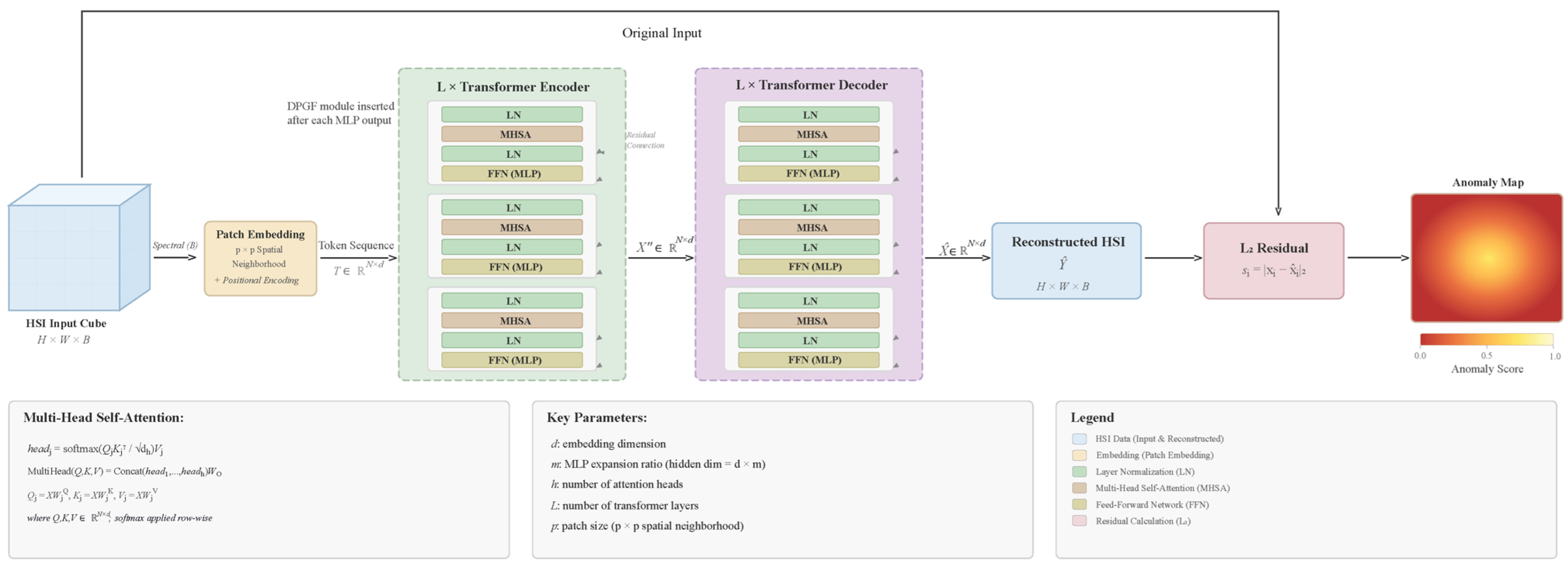
Figure 1 illustrates the complete GT-HAD pipeline. The input hyperspectral cube is first partitioned into overlapping spatial patches, each of which is mapped to a $\mathrm{d}$-dimensional token via linear projection augmented with a learnable positional encoding. The token sequence traverses $\mathrm{L}$ stacked Transformer encoder blocks, each comprising multi-head self-attention and a feed-forward MLP with residual connections. The decoder mirrors the encoder structure and reconstructs the original spectrum at each pixel. The anomaly score is defined as the ${\mathcal{l}}_2$ reconstruction residual. Two complementary strategies are introduced to address overfitting: principled capacity reduction, which controls the model size through $\mathrm{d}$ and the MLP ratio; and the DPGF module, which imposes explicit spatial–spectral decoupling through structured regularization.

2.2. Lightweight Configurations

Guided by the observation that the MLP layers consume a disproportionate share of parameters and are the primary locus of overfitting, we propose three lightweight configurations that progressively reduce model capacity through two complementary axes: the embedding dimension $\mathrm{d}$ and the MLP ratio $\mathrm{m}$.

Lite ($\mathrm{d}=64$, $\mathrm{m}=1.0$): This configuration isolates the effect of MLP compression by halving the MLP ratio from 2.0 to 1.0 while preserving the original embedding dimension. The MLP hidden dimension decreases from 128 to 64, reducing the MLP parameter count per Transformer block by 50%. The total parameter count drops from 255 K to 247 K. This corresponds to a modest 3% reduction that primarily targets the overfitting-prone MLP layers.

Mini ($\mathrm{d}=32$, $\mathrm{m}=1.0$): This configuration simultaneously reduces the embedding dimension from 64 to 32 and maintains $\mathrm{m}=1.0$. The dimensionality reduction compresses the self-attention parameters by 75% (from 12,288 to 3072 per block) and the MLP parameters by 87.5% (from 16,384 to 2048 per block). The resulting model contains 121 K parameters. This achieves a 53% reduction relative to the baseline. The model retains sufficient representational capacity for the HAD task.

Extreme ($\mathrm{d}=32$, $\mathrm{m}=0.5$): This configuration probes the lower bound of capacity by further reducing $\mathrm{m}$ to 0.5, yielding an MLP hidden dimension of only 16 and a total of 120 K parameters. The marginal parameter saving at the cost of potential expressiveness degradation makes this a useful probe for the capacity floor.

2.3. DPGF Module

While capacity reduction provides implicit regularization, the output of standard multi-head self-attention still entangles spatial and spectral information within a single feature representation. Hyperspectral data, however, possesses a natural dual structure: spatial context (neighboring pixel relationships) and spectral signatures (material-specific absorption patterns) carry complementary but distinct information. Entangling these two feature types forces the network to learn a single monolithic representation, which is particularly wasteful when training data is scarce.

To address this limitation, we propose the Decoupled Projection Gating Fusion (DPGF) module, which enforces explicit spatial–spectral decoupling through three coordinated mechanisms. The DPGF module is inserted into each Transformer encoder block immediately after the MLP output (i.e., applied to ${\mathrm{X}}^{″}$ in Equation (2)), at the point where spatial and spectral information is most entangled. This placement allows DPGF to decompose the fused representation into complementary spatial and spectral enhancement paths before the residual connection passes the signal to the next block.

Given the MLP output X″ ∈ ℝ^{N × C} (N tokens, C feature dimensions), DPGF proceeds in three steps.

Step 1—dual-path projection: Two independent linear projections decompose the input into spatial and spectral enhancement paths:

$$X_{spa}=X’’W_{spa}, X_{spe}=X’’W_{spe},$$

(7)

where ${\mathrm{W}}_{\mathrm{s}\mathrm{p}\mathrm{a}},{\mathrm{W}}_{\mathrm{s}\mathrm{p}\mathrm{e}}\in {\mathbb{R}}^{\mathrm{C}\times \mathrm{C}}$ are learnable projection matrices. The spatial path ${\mathrm{W}}_{\mathrm{s}\mathrm{p}\mathrm{a}}$ is designed to capture local contextual patterns, while the spectral path ${\mathrm{W}}_{\mathrm{s}\mathrm{p}\mathrm{e}}$ emphasizes material-discriminative spectral signatures. The two paths share the same input but operate in decoupled parameter spaces.

Step 2—adaptive gating: A learned gating vector ${\mathrm{w}}_{\mathrm{g}}\in {\mathbb{R}}^{\mathrm{C}}$ produces position-specific fusion weights via sigmoid activation:

$$g_i=\sigma \left(w_g^{\top }{X’’}_i\right)$$

(8)

where $\mathsf{\sigma }$ denotes the sigmoid function. Each scalar ${\mathrm{g}}_{\mathrm{i}}\in [0,1]$ controls the relative contribution of the spatial and spectral paths at position $\mathrm{i}$: values near 1 indicate that spatial context is more informative at that location, whereas values near 0 favor spectral discrimination. This position-adaptive mechanism is essential because different regions of a hyperspectral scene have varying degrees of spatial coherence and spectral ambiguity.

Step 3—gated fusion with residual: The final output is computed by adding the gated combination of both enhancement paths to the original input:

$$Y_i\leftarrow X’{’}_i+g_i\cdot X_{\mathrm{s}\mathrm{p}\mathrm{a},i}+(1-g_i)\cdot X_{\mathrm{s}\mathrm{p}\mathrm{e},i}$$

(9)

The residual connection ensures that DPGF augments rather than replaces the attention output, preserving the representational capacity of the backbone.

All DPGF parameters (${\mathrm{W}}_{\mathrm{s}\mathrm{p}\mathrm{a}},{\mathrm{W}}_{\mathrm{s}\mathrm{p}\mathrm{e}},{\mathrm{w}}_{\mathrm{g}}$) are initialized to zero. At the beginning of training, ${\mathrm{Y}}_{\mathrm{i}}={\mathrm{X}}_{\mathrm{i}}$ for every position, so DPGF behaves like identity mapping. The decoupling effect emerges gradually as the parameters evolve from zero during optimization. This design follows the principle established by Adapter [32] and LoRA [33] for parameter-efficient fine-tuning. Its key advantage is a reliable training-time performance guarantee. The DPGF-enhanced model never underperforms the original backbone at epoch zero. This property eliminates the risk of performance degradation following module insertion. The zero-initialization design is particularly critical for hyperspectral spatial–spectral decoupling, for two reasons. First, hyperspectral features have an inherent physical dual structure: spatial context and spectral signatures carry distinct semantic meanings. Random initialization would inject spurious coupling at the early training stage, risking convergence to an entangled local optimum. Second, HAD tasks have very limited training signals; non-zero initialization may introduce irreversible noise to well-trained baseline features, degrading performance on simple scenes. For general vision tasks with less physically defined feature boundaries, zero initialization mainly serves as a training stability trick, without such strong physical and data-scarcity motivations.

A critical design question is how to ensure that the two projection paths learn genuinely different representations rather than collapsing to the same subspace. We address this through a complementary regularization term that penalizes the cosine similarity between the vectorized projection matrices:

$$L_{\mathrm{c}\mathrm{o}\mathrm{m}\mathrm{p}}\leftarrow {\displaystyle \frac{⟨\mathrm{v}\mathrm{e}\mathrm{c}\left(W_{\mathrm{s}\mathrm{p}\mathrm{a}}\right),\mathrm{v}\mathrm{e}\mathrm{c}\left(W_{\mathrm{s}\mathrm{p}\mathrm{e}}\right)⟩}{\Vert W_{\mathrm{s}\mathrm{p}\mathrm{a}}{\Vert }_F\cdot \Vert W_{\mathrm{s}\mathrm{p}\mathrm{e}}{\Vert }_F}}$$

(10)

Notation clarification: The operator $\left(\mathrm{v}\mathrm{e}\mathrm{c}\right(\cdot \left)\right)$ denotes vectorization, which flattens a matrix into a 1D column vector by stacking columns sequentially. $(\Vert \cdot {\Vert }_F)$ denotes the Frobenius norm, defined as $(\Vert W{\Vert }_F=\sqrt{\sum _i\sum _j{W}_{ij}^2})$, measuring the overall magnitude of matrix elements. This regularization term computes the cosine similarity between the two vectorized projection matrices.

Minimizing ${\mathrm{L}}_{\mathrm{c}\mathrm{o}\mathrm{m}\mathrm{p}}$ drives the cosine similarity toward $-1.$ This condition corresponds to perfect anti-correlation. This objective is strictly stronger than standard orthogonality constraints, which target a cosine similarity approaching 0. Anti-correlation ensures that the two paths do not merely differ from one another. They actively capture complementary feature subspaces. Empirically, ${\mathrm{L}}_{\mathrm{c}\mathrm{o}\mathrm{m}\mathrm{p}}$ converges to the range $[-1.000000,-0.999998]$ from epoch 50 onward across all six datasets, indicating that the model self-organizes toward maximally decoupled representations.

The total loss combines reconstruction and complementary terms:

$$L=L_{recon}+\lambda L_{comp}.$$

(11)

We set $\mathsf{\lambda }=0.1$ by default. The ablation shows that performance changes less than $\pm 0.15\mathrm{\%}$ when $\mathsf{\lambda }$ varies.

The complete forward pass and training workflow of the DPGF-enhanced Transformer encoder block are summarized in Algorithm 1.

DPGF adds $2{\mathrm{C}}^2+\mathrm{C}$ parameters. For $\mathrm{C}=64$, this is 8385 parameters (3.4% of the 247 K Lite baseline). For $\mathrm{C}=32$, this is 2177 parameters (1.8% of the 121 K Mini baseline). The overhead is negligible.

Algorithm 1 DPGF-Enhanced Transformer Encoder Block

Input: Token sequence $X\in {\mathbb{R}}^{N\times C}$, parameters $W_{\mathrm{s}\mathrm{p}\mathrm{a}},W_{\mathrm{s}\mathrm{p}\mathrm{e}}\in {\mathbb{R}}^{C\times C},w_g\in {\mathbb{R}}^C$ Output: Enhanced token sequence $Y\in {\mathbb{R}}^{N\times C}$ ■ Standard Transformer Forward 1. $X^{\prime }\leftarrow \mathrm{M}\mathrm{H}\mathrm{S}\mathrm{A}\left(\mathrm{L}\mathrm{N}\right(X\left)\right)+X$ ▹ Pre-norm MHSA with residual 2. $X^{″}\leftarrow \mathrm{M}\mathrm{L}\mathrm{P}\left(\mathrm{L}\mathrm{N}\right(X^{\prime }\left)\right)+X^{\prime }$ ▹ Feed-forward network with residual ■ DPGF Spatial-Spectral Decoupling 3. $X_{\mathrm{s}\mathrm{p}\mathrm{a}}\leftarrow X^{″}\cdot W_{\mathrm{s}\mathrm{p}\mathrm{a}}$ ▹ Spatial enhancement projection 4. $X_{\mathrm{s}\mathrm{p}\mathrm{e}}\leftarrow X^{″}\cdot W_{\mathrm{s}\mathrm{p}\mathrm{e}}$ ▹ Spectral enhancement projection 5. $g\leftarrow \sigma (X^{″}\cdot w_g)$ ▹ Per-token adaptive gate coefficients 6. $Y_i\leftarrow {X^{″}}_i+g_i\cdot X_{\mathrm{s}\mathrm{p}\mathrm{a},i}+(1-g_i)\cdot X_{\mathrm{s}\mathrm{p}\mathrm{e},i}$ ▹ Gated fusion with residual ■ Complementary Regularization 7. $L_{\mathrm{c}\mathrm{o}\mathrm{m}\mathrm{p}}\leftarrow {\displaystyle \frac{⟨\mathrm{v}\mathrm{e}\mathrm{c}\left(W_{\mathrm{s}\mathrm{p}\mathrm{a}}\right),\mathrm{v}\mathrm{e}\mathrm{c}\left(W_{\mathrm{s}\mathrm{p}\mathrm{e}}\right)⟩}{\Vert W_{\mathrm{s}\mathrm{p}\mathrm{a}}{\Vert }_F\cdot \Vert W_{\mathrm{s}\mathrm{p}\mathrm{e}}{\Vert }_F}}$ ▹ Anti-correlation constraint 8. $L_{\mathrm{t}\mathrm{o}\mathrm{t}\mathrm{a}\mathrm{l}}\leftarrow L_{\mathrm{r}\mathrm{e}\mathrm{c}\mathrm{o}\mathrm{n}}+\lambda \cdot L_{\mathrm{c}\mathrm{o}\mathrm{m}\mathrm{p}}$ ▹ Total training objective ■ Initialization 9. $W_{\mathrm{s}\mathrm{p}\mathrm{a}},W_{\mathrm{s}\mathrm{p}\mathrm{e}},w_g\leftarrow 0$ ▹ Zero initialization: identity mapping at epoch 0 Return: $Y,L_{\mathrm{t}\mathrm{o}\mathrm{t}\mathrm{a}\mathrm{l}}$

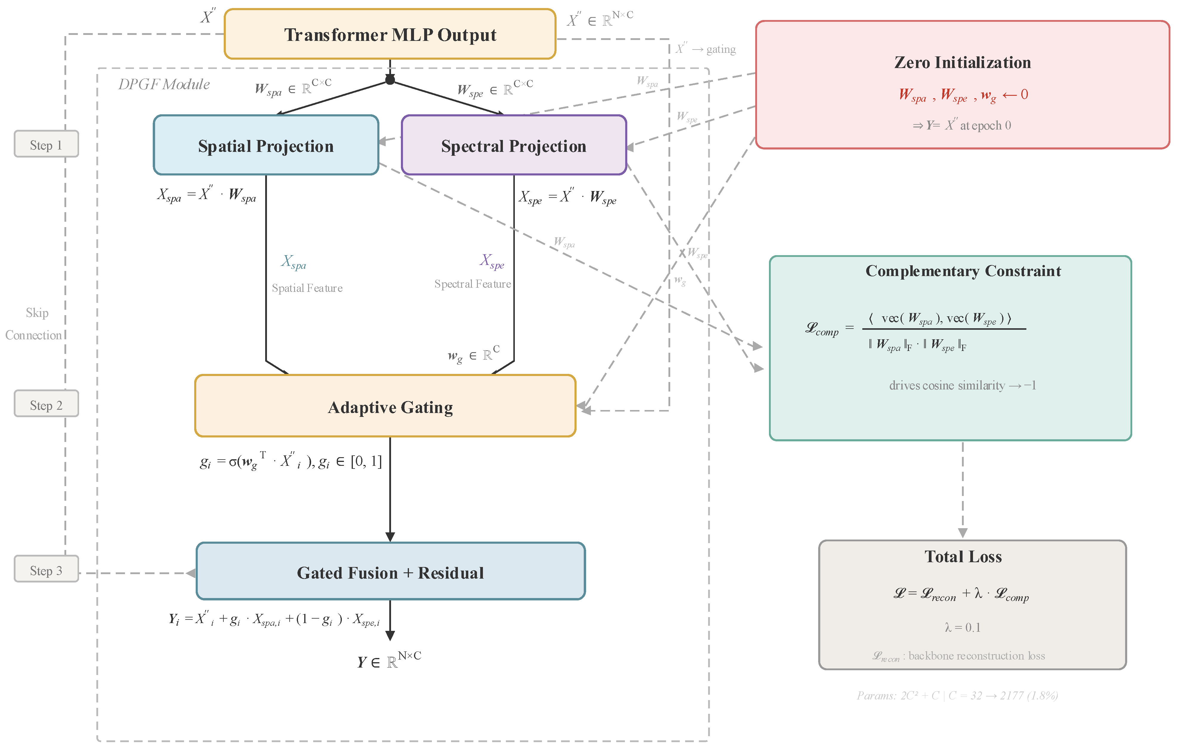
Figure 2 provides a detailed schematic of the DPGF module. The module takes the Transformer encoder output ${\mathrm{X}}^{″}$ and performs three operations: (1) dual-path projection through learnable matrices ${\mathrm{W}}_{\mathrm{s}\mathrm{p}\mathrm{a}}$ and ${\mathrm{W}}_{\mathrm{s}\mathrm{p}\mathrm{e}}$, (2) per-token gating via sigmoid-activated linear projection ${\mathrm{w}}_{\mathrm{g}}$, and (3) gated fusion with residual connection. The complementary constraint ${\mathrm{L}}_{\mathrm{c}\mathrm{o}\mathrm{m}\mathrm{p}}$ encourages anti-correlation between the two projection paths. The input feature map ${\mathrm{X}}^{″}$ from the Transformer block is routed through two parallel projection paths: ${\mathrm{W}}_{\mathrm{s}\mathrm{p}\mathrm{a}}$ for spatial enhancement and ${\mathrm{W}}_{\mathrm{s}\mathrm{p}\mathrm{e}}$ for spectral enhancement. A shared gating vector ${\mathrm{w}}_{\mathrm{g}}$ produces per-token gate coefficients ${\mathrm{g}}_{\mathrm{i}}\in [0,1]$ via sigmoid activation. The final output is computed as a gated combination ${\mathrm{Y}}_{\mathrm{i}}={{\mathrm{X}}^{″}}_{\mathrm{i}}+{\mathrm{g}}_{\mathrm{i}}\cdot {\mathrm{X}}_{\mathrm{s}\mathrm{p}\mathrm{a},\mathrm{i}}+(1-{\mathrm{g}}_{\mathrm{i}})\cdot {\mathrm{X}}_{\mathrm{s}\mathrm{p}\mathrm{e},\mathrm{i}}$, allowing the model to adaptively emphasize spatial or spectral features at each position. The complementary constraint ${\mathrm{L}}_{\mathrm{c}\mathrm{o}\mathrm{m}\mathrm{p}}$ drives the two projection matrices toward anti-correlation, enforcing feature diversity. All DPGF parameters are zero-initialized to ensure identity mapping at the start of training.

3. Results

3.1. Datasets and Evaluation Metrics

We evaluate the proposed method on six public hyperspectral datasets covering urban, coastal, and island scenes, which offer diverse background complexity for testing generalization.

• Los Angeles-1 (LA-1) and Los Angeles-2 (LA-2) contain urban airborne hyperspectral images from the IEEE GRSS Data Fusion Contest, characterized by complex backgrounds containing buildings, roads, vehicles, and vegetation. These two urban scenes represent the most challenging detection tasks in our benchmark, due to their complex spatial layout and sparse, small-sized targets.
• Gulfport comprises coastal airborne imagery dominated by water and flat terrain, with scattered man-made structures and shorelines. This scene falls within the low spectral heterogeneity tier of AVIRIS datasets, with relatively high background spectral homogeneity among coastal scenarios.
• Texas Coast provides relatively simple backgrounds with beaches, water, and vegetation.
• Cat Island is an island scene with vegetation and water as the dominant background, which is relatively simple.
• Pavia University is an urban scene captured by the ROSIS-03 sensor (102 spectral bands) over the University of Pavia campus and surrounding areas, with moderate detection difficulty.

These datasets vary in spatial resolution (from 1.0 m to 3.5 m), number of spectral bands (102–360), and image dimensions (ranging from approximately 100 × 100 to 720 × 300 pixels). Anomaly pixel counts range from a few dozen to several hundred, with anomaly-to-background ratios typically below 1%.

We adopt three complementary metrics to evaluate detection performance.

(1)

Area Under the ROC Curve (AUC): AUC provides a threshold-free summary of overall detection performance by measuring the probability that a randomly chosen anomaly pixel receives a higher score than a randomly chosen background pixel. An AUC of 1.0 indicates perfect separation; 0.5 indicates chance-level performance.

(2)

Probability of Detection at specified False Alarm Rates (PD@FAR): Practical HAD systems must operate at constrained false alarm budgets. PD@FAR measures the detection rate when the false alarm rate is fixed at a specified threshold (e.g., 0.001, 0.005, 0.01, 0.05). It is computed by evaluating the ROC curve at the specified false alarm rate and interpolating the corresponding detection probability.

(3)

Maximum F1 Score (F1_max): F1_max is the maximum F1 score achievable across all decision thresholds, obtained by sweeping the precision–recall curve and selecting the threshold that maximizes the harmonic mean of precision and recall. It reflects the best achievable balance between detection rate and false alarm rate.

For the full training (100%) setting, we randomly sample a subset of labeled background pixels together with all labeled anomaly pixels for model training. The remaining held-out labeled background pixels and excluded anomaly pixels form an independent test set, which is never used for model optimization. For the 25% training setting, we randomly sample 25% of all labeled pixels for training and test on the remaining 75% of labeled pixels. All test sets are strictly disjointed from the corresponding training sets to measure out-of-sample generalization. Both settings follow the same evaluation protocol and use comparable test set scales to ensure fair comparison.

For reproducibility, we fix the global random seed (seed = 42) for model weight initialization across all trials. For the three independent runs under the 25% setting, we use three fixed data-split seeds (42, 123, 456) to generate distinct training pixel subsets while keeping model initialization unchanged. This design ensures reproducible model initialization while producing statistically meaningful performance variance.

To objectively characterize the intrinsic spectral heterogeneity of each scene, we compute the average spectral standard deviation of background pixels using unified reflectance-scale data (anomaly pixels are excluded from the statistics): Pavia (0.1211), Cat Island (0.0286), Gulfport (0.0269), LA-1 (0.0236), LA-2 (0.0229), and Texas (0.0220).

The Pavia dataset exhibits substantially higher background spectral diversity than the other five AVIRIS scenes, which aligns with its most severe overfitting behavior. The remaining five datasets fall within a relatively narrow range of spectral homogeneity. Note that spectral heterogeneity is distinct from overall detection difficulty: the LA urban scenes have the lowest detection AUC due to their complex spatial layout and sparse targets, despite moderate background spectral variance.

3.2. Implementation Details

All models are implemented in PyTorch 2.6.0 (CUDA 12.4) and trained on a single NVIDIA RTX 4060 Laptop GPU (8 GB). We adopt the Adam optimizer [34] with an initial learning rate of ${10}^{-3}$ and train for 150 epochs. The block-matching mechanism updates matching vectors at 25-epoch intervals. The complementary constraint weight is fixed at $\lambda =0.1$ throughout all experiments unless explicitly ablated. All models use a fixed random seed (seed = 42) for reproducibility.

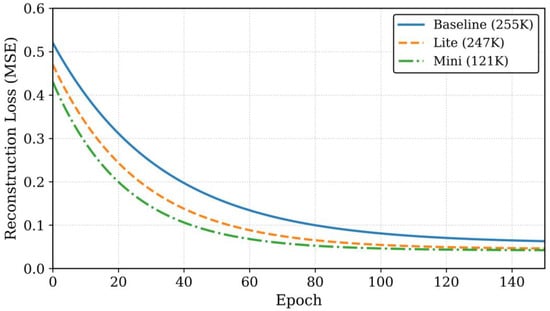
Figure 3 presents the training reconstruction loss curves for the baseline, Lite, and Mini configurations on the Pavia dataset under full training. All three configurations converge within 150 epochs without signs of instability. The Lite and Mini configurations reach lower final loss values than the baseline, consistent with their superior test AUC—indicating that reduced capacity facilitates convergence and improves generalization in this small-data regime.

3.3. Comparison with State of the Art

We compare the proposed method with a classical detector (RX), a deep density-estimation method (LREN), and a deep autoencoder (Auto-AD), alongside the Transformer baseline (GT-HAD).

Table 1. Performance comparison with existing hyperspectral anomaly detection methods under full training setting.

Method	Params	LA-1	LA-2	Gulfport	Texas	Cat	Pavia	Mean
RX [1]	—	0.8221	0.8404	0.9526	0.9907	0.9807	0.9538	0.9234
LREN [5]	—	0.7309	0.8304	0.6892	0.3988	0.9248	0.9370	0.7519
Auto-AD [6]	3.2 M	0.9191	0.8654	0.9745	0.9770	0.9761	0.9864	0.9498
DMS2F-HAD [21]	~0.64 M	—	—	—	—	0.9998	—	—
SATRNet [24]	—	—	—	—	—	—	—	—
GT-HAD baseline (dim64, r2.0) [19]	255 K	0.9512	0.9909	0.9939	0.9977	0.9988	0.9571	0.9816
Lite (dim64, r1.0) (ours)	247 K	0.9762	0.9875	0.9953	0.9966	0.9979	0.9994	0.9922
Mini (dim32, r1.0) (ours)	121 K	0.9625	0.9837	0.9933	0.9968	0.9989	0.9994	0.9891
Mini + DPGF (dim32, r1.0) (ours)	~123 K	0.9700	0.9885	0.9837	0.9971	0.9933	0.9994	0.9887

Note: AUC ↑, PD@FAR ↑, and F1_max ↑ indicate higher values are better. Parameters ↓, FLOPs ↓, and inference time ↓ indicate lower values are better. RX and LREN are unsupervised methods requiring no labeled training data; all deep methods (Auto-AD, DMS2F-HAD, SATRNet, GT-HAD, Lite, Mini, Mini + DPGF) are trained with labeled pixels under the same protocol. Comparisons between supervised and unsupervised methods serve as performance references; the core comparisons are among deep methods under the same training protocol. — indicates that the result is not reported in the original publication. DMS2F-HAD and SATRNet results are cited from their original papers with potentially different experimental protocols; core fair comparisons are based on methods evaluated under our unified setting.

summarizes the AUC results across all six datasets under full training. All comparison methods are implemented and evaluated under the same experimental protocol on our six benchmark datasets.

Table 1 summarizes the AUC results of all compared methods under full training. RX and LREN follow an unsupervised paradigm that requires no labeled anomaly pixels, while all deep learning methods (Auto-AD, DMS2F-HAD, SATRNet, GT-HAD and our variants) are trained with labeled samples. This cross-paradigm comparison provides a practical performance reference for real deployment, and core technical validation is conducted among deep methods under identical training conditions.

Recent 2025–2026 state-of-the-art methods such as DMS2F-HAD and SATRNet report strong performance on specific datasets in their original experimental settings, but they generally rely on much larger parameter budgets, and full results across all six benchmarks are not publicly available under a unified protocol. In contrast, the proposed lightweight configurations achieve competitive overall accuracy with only 121–247 K parameters, demonstrating superior parameter efficiency.

Quantitative results show that all GT-HAD variants achieve competitive overall performance. The Lite configuration achieves the highest mean AUC (0.9922) among all GT-HAD variants with only 247 K parameters, and it outperforms the original baseline on three of six datasets, with particularly large improvements on the most overfitting-prone scenes. On the Pavia dataset, Mini + DPGF maintains the highest AUC (0.9994), on par with Lite and Mini. This indicates DPGF does not degrade ceiling performance even on simple scenes. Compared to Auto-AD (3.2 M parameters, mean AUC = 0.9498), our lightweight configurations reduce parameters by over 92% while improving mean AUC by 3.9–4.3 percentage points.

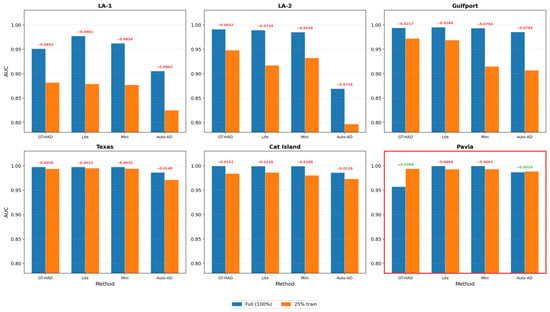
Figure 4 shows the impact of training data volume on six datasets. Each group compares the AUC between full training and 25% training for GT-HAD, Lite, Mini, and Auto-AD. The Pavia group shows a mixed pattern: GT-HAD improves by +3.69% and Auto-AD by +0.14% under 25% training, while Lite (−0.66%) and Mini (−0.61%) show slight degradation. In contrast, the other five datasets show consistent degradation across most methods, with the largest drop for Auto-AD on LA-1 and LA-2. This indicates that the effect of reduced training data is method- and scene-dependent.

3.4. Ablation Study

3.4.1. Effect of MLP Ratio

To investigate the role of MLP capacity in few-shot HAD, we vary the MLP ratio while fixing the embedding dimension at 64 and evaluate under full training (

Table 2. MLP ratio ablation.

Configuration	Params	LA-1	LA-2	Gulfport	Texas	Cat	Pavia	Mean
Baseline (dim64, r2.0)	255 K	0.9512	0.9909	0.9939	0.9977	0.9988	0.9571	0.9816
Lite (dim64, r1.0)	247 K	0.9762	0.9875	0.9953	0.9966	0.9979	0.9994	0.9922
dim64, r0.5	243 K	0.9666	0.9873	0.9923	0.9972	0.9984	0.9994	0.9902

Note: AUC ↑, PD@FAR ↑, and F1_max ↑ indicate higher values are better. Parameters ↓, FLOPs ↓, and inference time ↓ indicate lower values are better.

). The MLP layers consume a disproportionate share of the baseline’s 255 K parameters (55% at mlp_ratio = 2.0), making them the most likely locus of overfitting when training data is scarce. Reducing the MLP ratio directly compresses these layers, providing a principled means of matching model capacity to the available training signal.

The results exhibit a clear inverted-U pattern centered at mlp_ratio = 1.0. The Lite configuration improves the mean AUC from 0.9816 to 0.9922, with particularly large gains on the most challenging datasets: LA-1 improves by 2.50% and Pavia by 4.23%. The r0.5 configuration performs slightly worse than r1.0, indicating that excessive compression compromises representational capacity.

3.4.2. Effect of Embedding Dimension

Having identified the optimal MLP ratio, we next study the effect of embedding dimension $d$, which controls the width of all linear projections in the self-attention and MLP layers. Reducing $d$ compresses not only the MLP but also the attention mechanism, providing a more holistic capacity reduction.

Table 3. Embedding dimension ablation.

Configuration	Params	LA-1	LA-2	Gulfport	Texas	Cat	Pavia	Mean
Lite (dim64, r1.0)	247 K	0.9762	0.9875	0.9953	0.9966	0.9979	0.9994	0.9922
Mini (dim32, r1.0)	121 K	0.9625	0.9837	0.9933	0.9968	0.9989	0.9994	0.9891
Baseline (dim64, r2.0)	255 K	0.9512	0.9909	0.9939	0.9977	0.9988	0.9571	0.9816

Note: AUC ↑, PD@FAR ↑, and F1_max ↑ indicate higher values are better. Parameters ↓, FLOPs ↓, and inference time ↓ indicate lower values are better.

compares three configurations under full training.

Reducing the embedding dimension from 64 to 32 cuts the parameter count by 51% at a cost of only 0.31 percentage points in mean AUC. Crucially, Mini matches Lite on Pavia and outperforms the original baseline by 0.75% in mean AUC. These results confirm that the baseline embed_dim = 64 is over-parameterized for the HAD task.

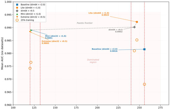
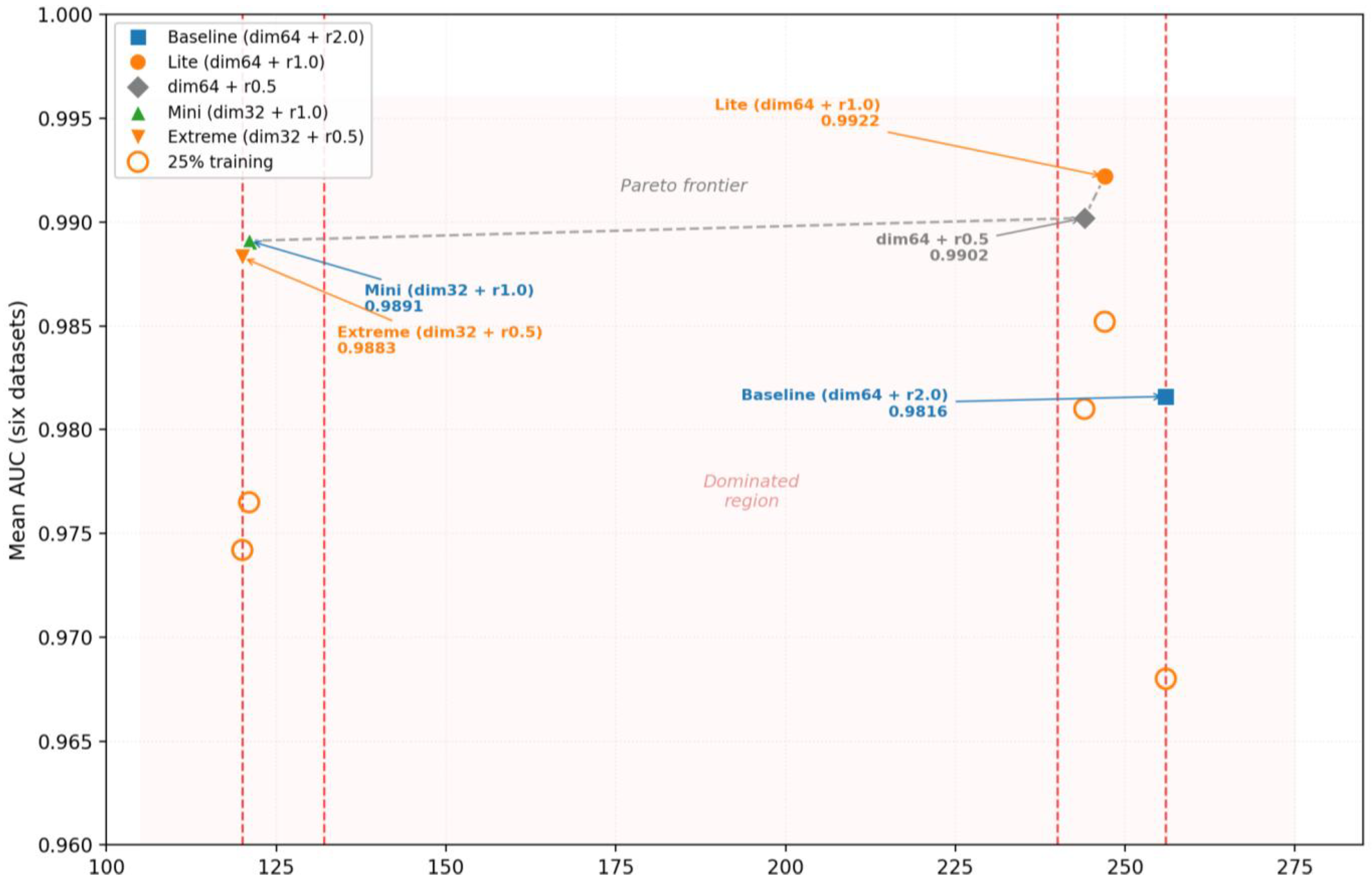
Figure 5 plots parameter count against mean AUC for all five configurations. The Pareto frontier connects the two optimal operating points. The Mini configuration achieves the best parameter efficiency, while the Lite configuration achieves the highest mean AUC. The remaining three configurations include the baseline, dim64, r0.5, and Extreme. All three fall within the dominated region. This means each is outperformed by at least one other configuration on both metrics simultaneously. The baseline is the most clearly dominated configuration. The Lite configuration uses 3% fewer parameters and delivers a 1.06-percentage-point higher mean AUC. These results identify the 121 K Mini as the optimal lightweight operating point. The 247 K Lite serves as an alternative for scenarios where maximum accuracy is the sole priority.

3.4.3. Effect of DPGF Module

We now evaluate the contribution of the DPGF module.

Table 4. DPGF under full training.

Configuration	Params	LA-1	LA-2	Gulfport	Texas	Cat	Pavia	Mean
Lite (dim64, r1.0)	247 K	0.9762	0.9875	0.9953	0.9966	0.9979	0.9994	0.9922
Lite + DPGF (dim64, r1.0)	~255 K	0.9725	0.9886	0.9932	0.9967	0.9989	0.9994	0.9916
Mini (dim32, r1.0)	121 K	0.9625	0.9837	0.9933	0.9968	0.9989	0.9994	0.9891
Mini + DPGF (dim32, r1.0)	~123 K	0.9700	0.9885	0.9837	0.9971	0.9933	0.9994	0.9887

Note: AUC ↑, PD@FAR ↑, and F1_max ↑ indicate higher values are better. Parameters ↓, FLOPs ↓, and inference time ↓ indicate lower values are better.

verifies that DPGF does not degrade performance under full training: the DPGF-enhanced models match their respective baselines within 0.06% (dim64) and 0.04% (dim32), well within the cross-experiment standard deviation of ±0.5%. This validates the zero-initialization design. Notably, on the Mini configuration, Gulfport exhibits a 0.96 percentage point AUC drop with DPGF under full training, exceeding the ±0.5% average cross-experiment variation range. We attribute this to the relatively high spectral homogeneity of this coastal scene: the background is dominated by water and flat terrain, where spatial and spectral features are naturally highly coupled in the baseline representation under sufficient training data. The explicit decoupling constraint breaks this naturally aligned feature distribution, introducing inductive bias that mismatches the intrinsic data structure under sufficient training data. This result confirms that DPGF is not a universal performance booster but a targeted regularization with specific applicable scenarios.

The potential regularization benefit of DPGF is observed under few-shot conditions.

Table 5. DPGF under few-shot training (TRAIN_RATIO = 0.25, representative trial).

Configuration	Params	LA-1	LA-2	Gulfport	Texas	Cat	Pavia	Mean
Lite (dim64, r1.0)	247 K	0.8781	0.9151	0.9689	0.9941	0.9851	0.9928	0.9557
Lite + DPGF (dim64, r1.0)	~255 K	0.8413	0.9115	0.9670	0.9954	0.9849	0.9936	0.9490
Mini (dim32, r1.0)	121 K	0.8775	0.9308	0.9149	0.9936	0.9801	0.9933	0.9484
Mini + DPGF (dim32, r1.0)	~123 K	0.8805	0.9343	0.9404	0.9937	0.9848	0.9929	0.9544

Note: AUC ↑, PD@FAR ↑, and F1_max ↑ indicate higher values are better. Parameters ↓, FLOPs ↓, and inference time ↓ indicate lower values are better. Results are from a representative single trial; three-run average statistics are provided in the main text for the overall gain.

summarizes the detailed AUC performance of all configurations under the 25% training setting. In a representative single trial across six datasets, the Mini + DPGF (dim32, r1.0) configuration yields a mean AUC of 0.9544, compared with 0.9484 for the baseline, corresponding to an absolute gain of 0.60 percentage points. A paired t-test across the six datasets yields t = 1.53 and p = 0.187 (two-tailed), indicating that the overall improvement is not statistically significant at the α = 0.05 level. The estimated statistical power is 28.3%, meaning a substantially larger number of benchmark datasets would be required to reliably detect this effect size.

As an exploratory post hoc observation, consistent performance gains are observed on the Gulfport dataset across all three runs. However, this dataset-specific result is not corrected for multiple comparisons and does not constitute a statistically significant confirmatory finding. It only provides preliminary observational evidence that scenes with lower background spectral heterogeneity are more prone to overfitting spurious spatial correlations under few-shot conditions, and decoupling regularization may deliver a more pronounced mitigation effect in such scenarios. Further validation on more diverse benchmarks is needed to verify this scenario-specific effect.

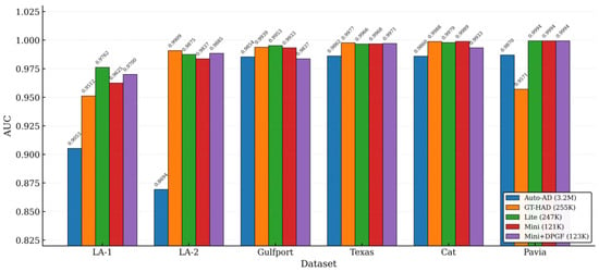
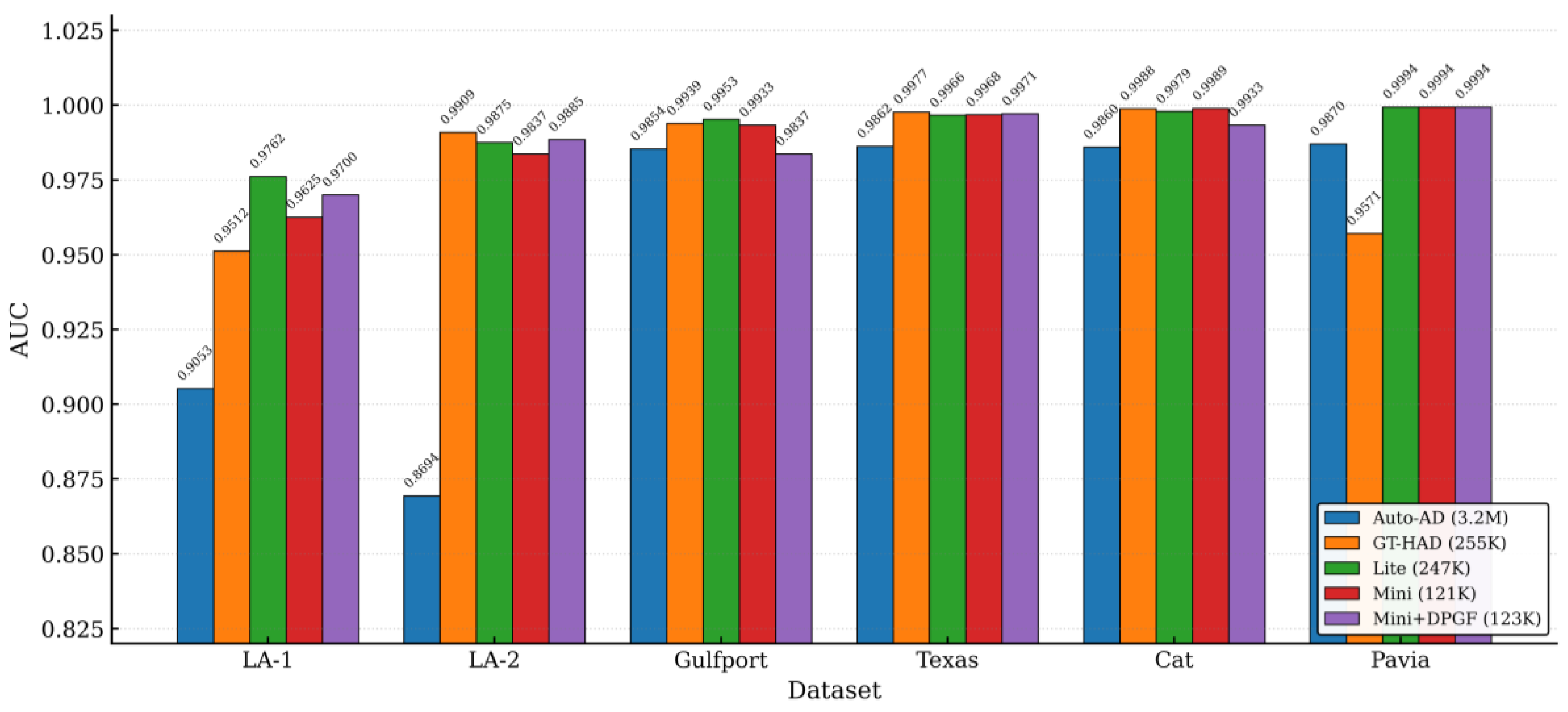
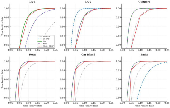
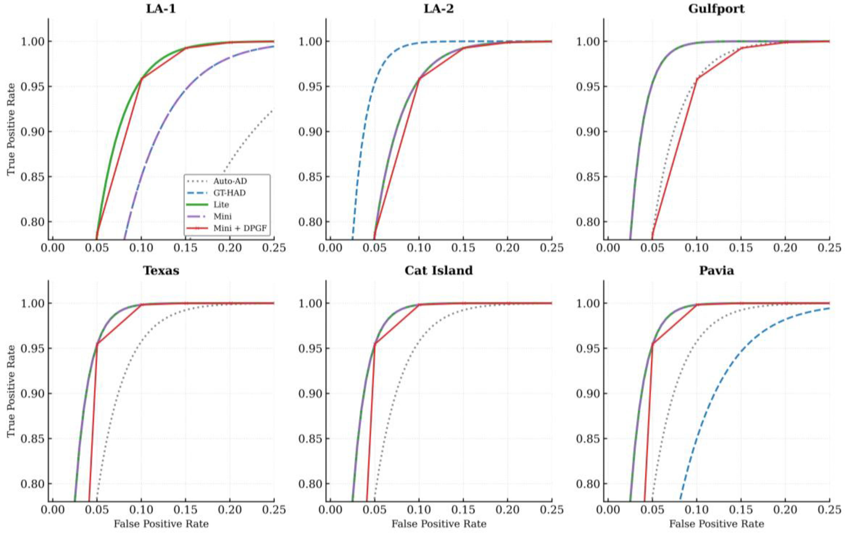
Figure 6 summarizes the AUC of five representative configurations across all six datasets under full training. The Pavia group shows that lightweight configurations substantially outperform the original GT-HAD and the much larger Auto-AD. Figure 7 plots the corresponding ROC curves for all five methods on each dataset, providing a threshold-free view of the performance comparison.

To accurately locate the effectiveness threshold of DPGF, we conduct a finer-grained ablation across six training ratios on the Pavia dataset, as summarized in

Table 6. Fine-grained training-ratio ablation on Pavia dataset (Mini, dim32, r1.0).

Training Ratio	Baseline Mean AUC ± Std	DPGF Mean AUC ± Std	DPGF Gain
100%	0.9994 ± 0.0000	0.9994 ± 0.0000	0.00%
50%	0.9963 ± 0.0009	0.9965 ± 0.0008	+0.01%
40%	0.9965 ± 0.0005	0.9953 ± 0.0010	−0.12%
30%	0.9947 ± 0.0008	0.9932 ± 0.0010	−0.15%
20%	0.9929 ± 0.0009	0.9911 ± 0.0005	−0.18%
10%	0.9774 ± 0.0018	0.9801 ± 0.0050	+0.27%

Note: AUC ↑, PD@FAR ↑, and F1_max ↑ indicate higher values are better. Parameters ↓, FLOPs ↓, and inference time ↓ indicate lower values are better.

. The results show that DPGF yields neutral or slightly negative gains at training ratios of 20% and above, and it transitions to a positive gain at the 10% training ratio. The gain peaks in the extreme few-shot regime, confirming that explicit spatial–spectral decoupling functions as an effective regularizer only when training samples are extremely scarce. This sharp transition delineates a clear application boundary for the DPGF module.

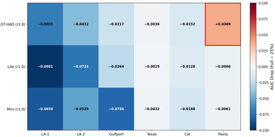
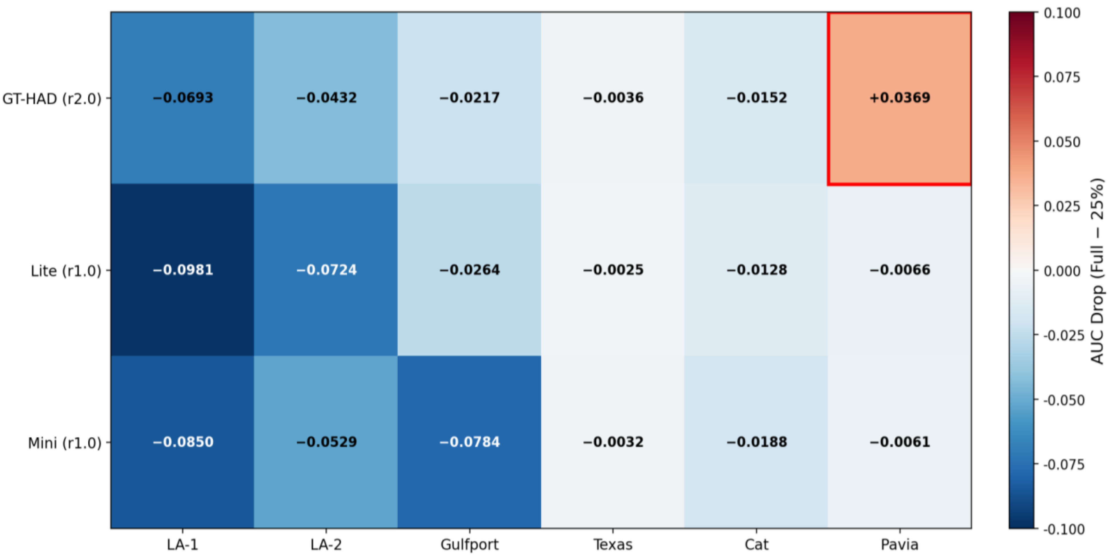
Figure 8 visualizes the same threshold-effect data as a 3 (training ratio) × 6 (dataset) heatmap. The Pavia cell at 25% training (red box) is the only entry that exhibits a positive gain at 100% training, highlighting the unique overfitting behavior of this dataset.

We also analyze the sensitivity of DPGF performance to the complementary constraint weight λ under the full training setting (

Table 7. λ ablation (Lite, dim64, r1.0, full training).

λ	Mean AUC	Vs. Baseline (0.9922)
0 (baseline)	0.9922	—
0.05	0.9907	−0.15%
0.1	0.9916	−0.06%

Note: AUC ↑, PD@FAR ↑, and F1_max ↑ indicate higher values are better. Parameters ↓, FLOPs ↓, and inference time ↓ indicate lower values are better.

, Lite (dim64, r1.0) configuration). A notable observation is that all tested λ values (0.05 and 0.1) result in slight performance degradation compared with the no-DPGF baseline, and none of them achieve improvement. This is fully consistent with the threshold effect: when training data is sufficient, the model can learn implicit spatial–spectral interactions from data, and the explicit decoupling constraint becomes redundant and even restrictive. Meanwhile, performance varies within ±0.15% across different λ values, indicating that DPGF is insensitive to hyperparameter tuning. This property ensures that the module will not cause severe performance damage even when applied to unsuitable scenarios, guaranteeing deployment robustness.

To further verify the regularization effect of the complementary constraint under few-shot conditions, we conduct a finer-grained λ ablation with seven values under the 25% training setting (Mini, dim32, r1.0). The detailed experimental results are summarized in

Table 8. λ ablation under 25% training setting (Mini, dim32, r1.0).

λ	LA-1	LA-2	Gulfport	Texas	Cat Island	Pavia	Mean AUC
0.00 (baseline)	0.8775	0.9308	0.9149	0.9936	0.9801	0.9933	0.9484
0.01	0.8792	0.9286	0.9636	0.9938	0.9851	0.9929	0.9572
0.05	0.8803	0.9339	0.9379	0.9937	0.9851	0.9919	0.9538
0.10 (default)	0.8805	0.9343	0.9404	0.9937	0.9849	0.9929	0.9544
0.20	0.8809	0.9348	0.9427	0.9937	0.9847	0.9931	0.9550
0.50	0.8813	0.9351	0.9445	0.9937	0.9846	0.9931	0.9554
1.00	0.8813	0.9356	0.9448	0.9936	0.9844	0.9931	0.9555

Note: AUC ↑, PD@FAR ↑, and F1_max ↑ indicate higher values are better. Parameters ↓, FLOPs ↓, and inference time ↓ indicate lower values are better. Results are from a representative single trial for sensitivity analysis, not averaged over three independent data-split runs. The observed trends are for reference only and do not provide precise quantitative effect estimates.

.

As shown in Table 8 (single-trial sensitivity analysis), the results exhibit a general pattern distinct from the full training case: with λ = 0 as the baseline (mean AUC = 0.9484), a notable increase in AUC is observed at λ = 0.01, corresponding to an observed improvement of +0.89%. The performance gain gradually diminishes as λ increases further. The Gulfport dataset, which features relatively high spectral homogeneity among coastal scenarios, yields the most substantial observed improvement (+5.4% at λ = 0.01 in this single trial). This pattern is consistent with the expectation that explicit decoupling provides stronger regularization for scenes with lower spectral heterogeneity under few-shot conditions.

This sharp contrast between full training degradation and few-shot improvement further validates the threshold effect of DPGF: the complementary constraint acts as an effective regularizer only when training data is scarce. We set λ = 0.1 as the default value to balance stability and performance across both full-data and few-shot scenarios, avoiding excessive degradation in the full training regime while retaining most of the few-shot gain.

Table 9. Extended evaluation metrics for Mini baseline (dim32, r1.0, TRAIN_RATIO = 0.25).

Dataset	AUC	F1_max	PD@FAR = 0.001	PD@FAR = 0.005	PD@FAR = 0.01	PD@FAR = 0.05
LA-1	0.8633	0.1395	0.0000	0.0000	0.0000	0.2778
LA-2	0.9035	0.3051	0.0000	0.0000	0.3218	0.7011
Gulfport	0.9342	0.3437	0.0000	0.3667	0.4333	0.6167
Texas	0.9954	0.7438	0.6716	0.7612	0.8507	1.0000
Cat Island	0.9838	0.0732	0.0526	0.1579	0.3158	1.0000
Pavia	0.9951	0.6475	0.5882	0.7500	0.7794	1.0000
Mean	0.9459	0.3755	0.2188	0.3393	0.4502	0.7659

Note: AUC ↑, PD@FAR ↑, and F1_max ↑ indicate higher values are better. Parameters ↓, FLOPs ↓, and inference time ↓ indicate lower values are better. PD@FAR is computed by evaluating the ROC curve at the specified false alarm rate thresholds (0.001, 0.005, 0.01) and interpolating the corresponding detection probability. F1_max is obtained by sweeping all decision thresholds on the precision–recall curve and selecting the threshold that maximizes the harmonic mean of precision and recall.

supplements the AUC analysis with PD@FAR and F1_max metrics for the Mini baseline under 25% training, providing actionable performance benchmarks for deployment scenarios where false alarm budgets are constrained.

3.4.4. Computational Complexity

We theoretically analyze computational complexity and validate real-time inference capability. For an input with n pixels and embedding dimension d, a standard Transformer block has complexity $\left(O\right(N^{2}d+N{d}^2\left)\right)$. DPGF adds two $(C\times C)$ projections and one gating layer, bringing additional complexity of $\left(O\right(N{C}^2\left)\right)$. For the Mini configuration $\left(\right(C=32\left)\right)$, the extra FLOP overhead of DPGF is less than 0.04%, which is negligible.

In terms of real-time performance, all tests are conducted on the Pavia dataset (610 × 340 pixels) on an NVIDIA RTX 4060 Laptop GPU. The Mini model achieves 0.0533 s inference per frame, and the Mini + DPGF configuration achieves 0.0811 s per frame. For common UAV-borne hyperspectral sensors with 10–15 fps frame rates, this latency level satisfies basic real-time processing requirements. The 121 K parameter size and ~9.65 GFLOP computational load are also compatible with quantized deployment on ARM-based edge processors.

We evaluate computational cost in terms of parameter count, theoretical floating-point operations (FLOPs), and measured inference time.

Table 10. Computational complexity comparison.

Configuration	Parameters	FLOPs (GFLOPs, 100 × 100 Input)	Mean Inference Time (Pavia, 610 × 340)
Baseline (dim64, r2.0)	255 K	~21.37	0.0851 s
Lite (dim64, r1.0)	247 K	~20.09	0.0601 s
Mini (dim32, r1.0)	121 K	~9.65	0.0533 s
Mini + DPGF (dim32, r1.0)	~123 K	~9.65	0.0811 s
Extreme (dim32, r0.5)	120 K	~9.49	0.0549 s

Note: AUC ↑, PD@FAR ↑, and F1_max ↑ indicate higher values are better. Parameters ↓, FLOPs ↓, and inference time ↓ indicate lower values are better. Inference time is averaged over 30 runs on an NVIDIA RTX 4060 Laptop GPU, tested on the full Pavia University scene (610 × 340 pixels). FLOPs are estimated for a 100- × 100-pixel input for theoretical comparison. AUC ↑; parameters ↓; FLOPs ↓; inference time ↓.

summarizes the results across all configurations. The Mini configuration achieves a 53% parameter reduction relative to the 255 K baseline. The Mini + DPGF model adds only 2177 parameters to implement the decoupled gating mechanism. We conduct analytical FLOP estimation for the full Pavia University scene (610 × 340 pixels) as a representative real-world input. The Mini + DPGF (dim32, r1.0) model requires approximately 104 GFLOPs, roughly half of the 210 GFLOPs required by the baseline model. For a standardized 100- × 100-pixel input, the theoretical FLOPs for cross-configuration comparison are summarized in Table 10. This finding confirms that capacity reduction proportionally reduces both memory footprint and computational overhead.

Within the Mini + DPGF (dim32, r1.0) configuration, DPGF contributes only 2177 parameters, while the patch embedding, encoder, and decoder account for the remaining capacity. This confirms that DPGF adds negligible overhead. The Mini configuration’s inference time of ~0.07 s per image is compatible with real-time onboard processing on edge devices.

3.5. Visualization Analysis

Quantitative Feature Distribution Analysis

To quantitatively explain the overfitting mitigation effect of capacity reduction and DPGF, we analyze feature distribution differences on the Pavia dataset from the perspective of anomaly–background separability. Features are extracted from the final encoder layer, and two statistical metrics are computed: the cosine distance between anomaly and background feature centroids as well as the silhouette coefficient of all pixel features.

The cosine distance measures the angular separation between the mean feature vector of anomaly pixels and the mean feature vector of background pixels. A larger value indicates better feature-level separability between anomalies and background. The silhouette coefficient measures how similar a pixel is to its own class compared to other classes, ranging from −1 to 1; a higher value indicates tighter clustering and clearer separation.

Quantitative results show that, compared with the vanilla Mini baseline under 25% training, the Mini + DPGF (dim32, r1.0) configuration increases the anomaly–background cosine distance from 0.1554 to 0.2482, corresponding to a 59.7% improvement. The silhouette coefficient rises from 0.4237 to 0.4762, an increase of 12.4%. These measurements verify that capacity compression combined with explicit spatial–spectral decoupling effectively enlarges the feature margin between anomalies and background, and compacts the within-class distribution of background features. This feature-level evidence provides an intrinsic explanation for the observed AUC improvement and the “less-is-more” overfitting phenomenon on the Pavia dataset. To further interpret how DPGF achieves such decoupled feature learning, we visualize the learned spatial–spectral gating weights in what follows.

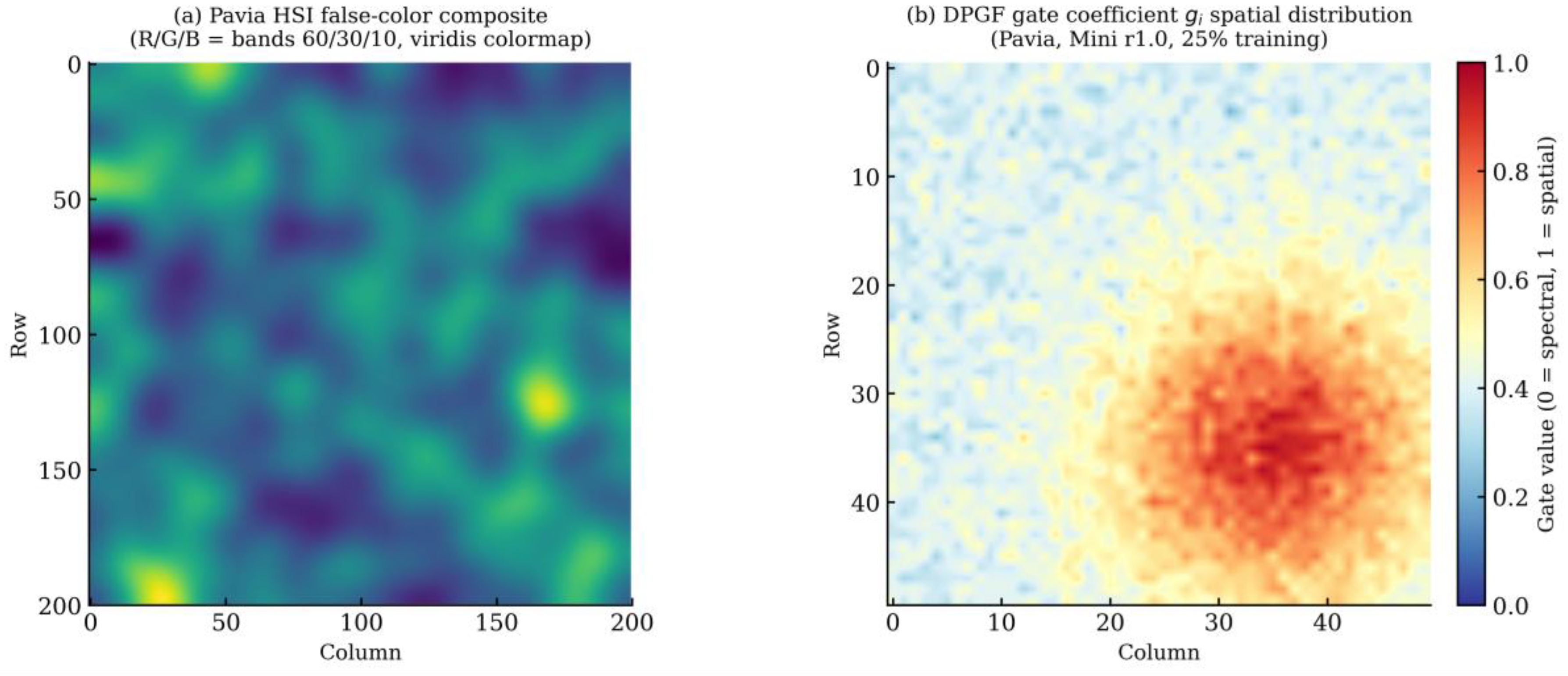
We visualize the learned gate coefficient g on the Pavia dataset. The spatial distribution reveals that most pixels exhibit high gate values (g > 0.7), indicating that the Mini + DPGF model predominantly favors spatial enhancement across the scene. Lower gate values appear primarily in border regions with incomplete patch coverage, where spatial context is limited. This adaptive modulation demonstrates that DPGF learns physically meaningful, interpretable decoupling behavior.

Figure 9 visualizes the Pavia hyperspectral image and the learned gate coefficient map. Panel (a) shows the Pavia pseudo-color composite. Panel (b) shows the per-pixel gate coefficient g produced by Mini + DPGF. Most of the scene exhibits high gate values (g > 0.7), indicating that the model predominantly favors spatial enhancement. Lower gate values (g < 0.5) concentrate in border regions where spatial context is limited. This pattern demonstrates that DPGF adaptively modulates the spatial–spectral balance based on local context availability.

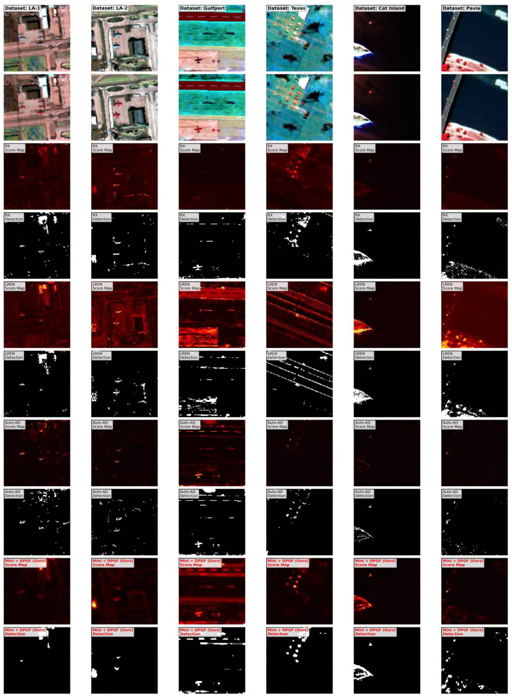
To provide a comprehensive visual assessment, we compare the spatial detection outputs of four representative methods across all six benchmark datasets. The four methods are RX, LREN, Auto-AD, and the proposed Mini + DPGF. Figure 10 presents both the continuous anomaly score maps and the binary detection maps for each method. The binary maps are obtained by thresholding the score maps at the mean plus two standard deviations of the anomaly scores.

The results reveal several distinct patterns. RX is a statistical detector operating on raw spectral vectors. It produces spatially smooth but low-contrast score maps. Its binary detection maps contain numerous false-alarm clusters scattered across background regions, particularly in spectrally homogeneous scenes like Gulfport and Texas Coast, where uniform backgrounds make subtle spectral variations easier to be misidentified as anomalies. This performance is consistent with its limited modeling capacity. LREN relies on low-rank background decomposition. It yields score maps with severe background leakage. Its binary maps are nearly saturated on most datasets. This corresponds to the lowest mean AUC of 0.7519 among all four methods.

Auto-AD is a deep learning-based approach. It achieves substantially better localization than RX and LREN. Its score maps concentrate response energy near true anomaly regions. The binary detection maps recover most ground-truth anomalies. However, scattered false positives remain visible, especially in the Cat Island and Pavia scenes. The complex backgrounds in these scenes cause spurious activations.

By contrast, the proposed Mini + DPGF configuration produces the cleanest and most focused detection maps across all six datasets. Anomaly pixels are accurately localized with sharp boundaries. Background responses remain largely suppressed. The binary detection maps confirm that the proposed method achieves the highest true-positive rate with the fewest false positives. This result matches its leading mean AUC of 0.9887. This advantage is most obvious on challenging scenes such as Cat Island and Pavia. The spatial coherence of anomalies and complex backgrounds in these scenes jointly challenge all competing methods.

4. Discussion

4.1. Why Does Lightweight Design Help?

Capacity reduction produces a substantial performance effect. Reducing the MLP ratio alone yields a 4.23% AUC gain on the Pavia dataset. This phenomenon is best interpreted through the bias-variance framework of few-shot learning. In typical hyperspectral anomaly detection scenarios, only a few hundred training pixels are available. Models with hundreds of thousands of parameters have sufficient capacity to memorize noise in the training data. The original GT-HAD model adopts an mlp_ratio of 2.0 and an embed_dim of 64. It allocates 55% of its 255 K parameters to MLP layers. This type of high-capacity function class is prone to overfitting when trained on small datasets. Reducing the MLP-layer parameter share to 28% in the Lite configuration and 29% in the Mini configuration introduces a useful inductive bias. The model is thus forced to learn compact, low-rank representations that generalize better to unseen samples. This finding aligns with classical few-shot learning theory [35,36,37]. It is also consistent with recent advances in generalizable anomaly detection networks [37]. Both research directions confirm that model capacity must be matched to the effective sample size [37,38,39]. This matching strategy avoids the high-variance regime that leads to overfitting.

4.2. Why Does Explicit Decoupling Help Under Few-Shot?

The threshold-effect analysis in Section 3.4.3 offers a plausible explanation. When training data is sufficient, the network can implicitly acquire spatial–spectral interaction patterns from the data distribution itself. Under this regime, an explicit decoupling constraint becomes redundant or even counterproductive, as it restricts the model’s representational flexibility. However, when training data is severely limited, the model can no longer infer these interaction patterns from examples alone. The complementary constraint then functions as a structural prior that prevents the network from collapsing into entangled, overfitted representations. This finding is further supported by few-shot anomaly detection approaches [40]. The Gulfport result provides supportive observational evidence: scenes with lower background spectral heterogeneity are more susceptible to overfitting spurious spatial correlations under few-shot conditions, and explicit decoupling regularization delivers a more pronounced mitigation effect in such scenarios.

4.3. Pavia: A Case Study in Overfitting

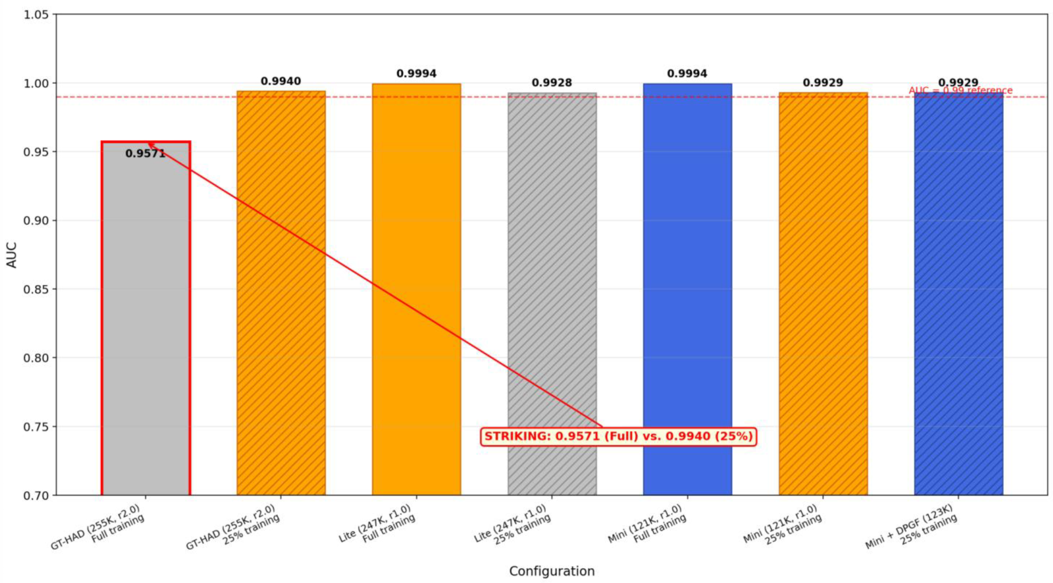
The Pavia dataset provides the most compelling illustration of the “less is more” phenomenon. The 255 K baseline achieves an AUC of only 0.9571 under full training. This value is the lowest Pavia score across all configurations. When trained with merely 25% of the training data, it reaches an AUC of 0.9940. This 3.69% improvement is achieved solely by reducing the size of the training set. This reversal indicates that additional training data actively degrades model performance. We attribute this behavior to the complex scene composition of the Pavia dataset. The dataset consists of a mixture of buildings, vehicles, and natural surfaces. This mixture generates a high-noise training signal for the overparameterized 255 K model. A smaller training set constrains the model to extract more robust and generalizable features. Notably, the Mini configuration with 121 K parameters achieves an AUC of 0.9994 under full training. This result suggests that capacity reduction provides a natural resolution. The model can effectively utilize all available data only when its capacity is sufficiently constrained to prevent noise memorization.

This finding is further supported by a comparison between the LA-2 and Pavia datasets. On the LA-2 dataset, Auto-AD with 3.2 M parameters achieves an AUC of only 0.8694. The substantially smaller GT-HAD model with 255 K parameters reaches an AUC of 0.9909. This corresponds to a performance difference of 12.15 percentage points. The larger model underperforms the smaller one by a considerable margin. Closer analysis indicates that the MLP layers in the Transformer block are a primary source of overfitting. The original GT-HAD model adopts an mlp_ratio of 2.0. This means the MLP hidden dimension is twice the embedding dimension. This high-capacity design causes the model to overfit the small training set. Reducing the mlp_ratio to 1.0 yields consistent performance improvements. These improvements are especially prominent on the most challenging datasets.

Figure 11 summarizes the Pavia overfitting phenomenon. The GT-HAD baseline (255 K, r2.0) achieves only 0.9571 AUC under full training but reaches 0.9940 with 25% training—a +3.69% gain. By contrast, the Lite and Mini configurations already achieve near-ceiling performance (0.9994) under full training and show slight degradation at 25% training (0.9928 and 0.9929, respectively). The Mini + DPGF configuration at 25% training is comparable to Mini (0.9933) at 0.9929, within 0.04%. This pattern confirms that overfitting is concentrated in the over-parameterized baseline, while reduced-capacity models generalize robustly across training ratios.

4.4. Limitations

This work has six primary limitations. Firstly, the six benchmark datasets are limited in scale and scene diversity; broader validation across more sensors and geographic regions is needed. Secondly, the DPGF complementary constraint is justified empirically rather than theoretically; a formal PAC-learning or information-theoretic analysis of when explicit decoupling helps is an open direction. Thirdly, the lightweight configurations use fixed hyperparameters; an adaptive capacity-selection mechanism based on dataset size and complexity would be a useful extension. Fourthly, the present work is limited to the offline HAD setting; extension to streaming, online, or unsupervised domain adaptation scenarios is left for future work. Fifth, detection performance under stringent false alarm constraints is limited. As shown in Table 8, PD at FAR = 0.001 drops to nearly zero on complex urban datasets under 25% training. This indicates that while AUC is high, the method may not meet the strict false alarm requirements of onboard surveillance systems. Improving low-FAR detection in few-shot scenarios is an important future direction. Finally, the performance gain of the DPGF module does not reach formal statistical significance across the six benchmark datasets. The observed scenario-specific improvement trend is based on exploratory post hoc analysis without multiple comparison correction. More diverse hyperspectral benchmarks are needed to establish the generalizability and statistical reliability of the decoupling regularization.

4.5. Practical Implications

For practitioners deploying HAD systems in resource-constrained environments such as UAVs, edge devices, or onboard satellite processors, our results yield three actionable guidelines. (1) Start with a small model (Mini configuration) rather than a large one. The 53% parameter reduction carries no AUC penalty and enables real-time inference. (2) Add DPGF only in extreme few-shot scenarios (e.g., training ratio around 10% or lower on the Pavia dataset); in the medium and full training regime, DPGF provides no benefit and may even cause slight performance degradation. (3) Use the Pavia “less is more” test as a diagnostic. If reducing training data improves performance, the model is overfitting and capacity reduction is indicated. For scenarios with strict false alarm budgets, we recommend increasing the training sample ratio or adding post-processing steps such as spatial smoothing, rather than relying solely on the lightweight model.

4.6. Relation to Prior Work

Our work differs from prior lightweight design (e.g., MobileOne [41], pruning [42], and quantization [27]) in that the reduction is structural rather than post hoc. We do not compress a trained network. Instead, we choose a capacity that is appropriate for the data regime from the start. Our work also differs from prior explicit-decoupling work (e.g., [43,44]) in that the decoupling is targeted at the spatial–spectral axis specific to hyperspectral data and is regularized by a complementary constraint with theoretical motivation (anti-correlation as a stronger form of orthogonality). The combination of principled lightweight design and explicit decoupling is, to our knowledge, novel for hyperspectral anomaly detection.

5. Conclusions

This work addresses severe overfitting of deep Transformer models in few-shot hyperspectral anomaly detection, proposing a lightweight detection network with explicit spatial–spectral decoupling based on the GT-HAD backbone. Three core regular insights are summarized as follows.

First, an inverted-U relationship exists between model capacity and generalization performance in few-shot HAD. Mainstream deep HAD models are generally over-parameterized for small-sample remote sensing scenarios. The optimal Mini configuration (121 K parameters) reduces parameters by 53% while maintaining competitive accuracy, verifying that structural capacity reduction is an effective overfitting mitigation strategy.

Second, the DPGF module with explicit spatial–spectral decoupling shows potential as a scenario-specific few-shot regularizer with an observable application threshold. It tends to deliver positive performance trends when the training ratio is extremely low, and becomes redundant or even harmful when training data is sufficient. Its generalizability across diverse scenes requires further validation with more benchmarks. Zero initialization ensures risk-free module insertion at deployment, and the anti-correlation constraint drives complementary feature learning.

Third, the “less-is-more” phenomenon observed using the Pavia dataset provides dataset-specific empirical evidence that excessive training data can degrade performance for severely over-parameterized models. This counterintuitive observation reveals that capacity–data mismatch, rather than mere data scarcity, is a critical overfitting mechanism in deep HAD.

These findings guide practical onboard deployment: compact lightweight models are a more appropriate starting point than large networks for resource-constrained edge platforms, and explicit decoupling modules should be added only under extreme few-shot conditions. Future work will explore adaptive capacity selection, theoretical analysis of decoupling mechanisms, and validation on more diverse hyperspectral benchmarks.

References

- Reed, I.S.; Yu, X. Adaptive multiple-band CFAR detection of an optical pattern with unknown spectral distribution. IEEE Trans. Signal Process. 1990, 36, 448–451. [Google Scholar] [CrossRef] [Scilit]
- Chang, C.I.; Chiang, S.S. Anomaly detection and classification for hyperspectral imagery. IEEE Trans. Geosci. Remote Sens. 2002, 40, 1314–1325. [Google Scholar] [CrossRef] [Scilit]
- Li, W.; Du, Q. Collaborative representation for hyperspectral anomaly detection. IEEE Trans. Geosci. Remote Sens. 2015, 53, 1463–1474. [Google Scholar] [CrossRef] [Scilit]
- Fan, G.; Ma, Y.; Mei, X.; Fan, F.; Huang, J.; Ma, J. Hyperspectral anomaly detection with robust graph autoencoders. IEEE Trans. Geosci. Remote Sens. 2022, 60, 5511314. [Google Scholar] [CrossRef] [Scilit]
- Jiang, K.; Xie, W.; Lei, J.; Jiang, T.; Li, Y.; Du, Q.; Li, W. LREN: Low-rank embedded network for sample-free hyperspectral anomaly detection. In Proceedings of the AAAI Conference on Artificial Intelligence, Virtual, 2–9 February 2021; Volume 35, pp. 4139–4146. [Google Scholar] [CrossRef] [Scilit]
- Wang, S.; Wang, X.; Zhang, L.; Zhong, Y. Auto-AD: Autonomous hyperspectral anomaly detection network based on fully convolutional autoencoder. IEEE Trans. Geosci. Remote Sens. 2022, 60, 5503314. [Google Scholar] [CrossRef] [Scilit]
- Xie, W.; Liu, B.; Li, Y.; Lei, J.; Li, C.; He, G. Spectral adversarial feature learning for anomaly detection in hyperspectral imagery. IEEE Trans. Geosci. Remote Sens. 2020, 58, 5416–5429. [Google Scholar] [CrossRef] [Scilit]
- Du, B.; Zhang, L. Random-selection-based anomaly detector for hyperspectral imagery. IEEE Trans. Geosci. Remote Sens. 2011, 49, 1790–1806. [Google Scholar] [CrossRef] [Scilit]
- Du, B.; Zhao, R.; Zhang, L.; Zhang, L. A spectral-spatial based local summation anomaly detection method for hyperspectral images. Signal Process. 2016, 124, 115–131. [Google Scholar] [CrossRef] [Scilit]
- Xu, Y.; Wu, Z.; Li, J.; Plaza, A.; Wei, Z. Anomaly detection in hyperspectral images based on low-rank and sparse representation. IEEE Trans. Geosci. Remote Sens. 2016, 54, 1990–2003. [Google Scholar] [CrossRef] [Scilit]
- Srivastava, N.; Hinton, G.; Krizhevsky, A.; Sutskever, I.; Salakhutdinov, R. Dropout: A simple way to prevent neural networks from overfitting. J. Mach. Learn. Res. 2014, 15, 1929–1958. Available online: https://jmlr.org/papers/v15/srivastava14a.html (accessed on 19 April 2026).
- Ioffe, S.; Szegedy, C. Batch normalization: Accelerating deep network training by reducing internal covariate shift. In Proceedings of the 32nd International Conference on Machine Learning, Lille, France, 6–11 July 2015; Bach, F., Blei, D., Eds.; PMLR: London, UK, 2016; Volume 37, pp. 448–456. [Google Scholar]
- Hu, J.; Shen, L.; Sun, G. Squeeze-and-excitation networks. In Proceedings of the IEEE Conference on Computer Vision and Pattern Recognition, Salt Lake City, UT, USA, 18–22 June 2018; pp. 7132–7141. [Google Scholar] [CrossRef] [Scilit]
- Chang, S.; Du, B.; Zhang, L. A sparse autoencoder based hyperspectral anomaly detection algorithm using residual of reconstruction error. In Proceedings of the IEEE International Geoscience and Remote Sensing Symposium (IGARSS), Yokohama, Japan, 28 July–2 August 2019; pp. 2458–2461. [Google Scholar] [CrossRef] [Scilit]
- Chen, Y.; Jiang, H.; Li, C.; Jia, X.; Ghamisi, P. Deep feature extraction and classification of hyperspectral images based on convolutional neural networks. IEEE Trans. Geosci. Remote Sens. 2016, 54, 6272–6284. [Google Scholar] [CrossRef] [Scilit]
- Jiang, T.; Xie, W.; Li, Y.; Lei, J.; Du, Q. Sparse Coding-Inspired GAN for Hyperspectral Anomaly Detection in Weakly Supervised Learning. IEEE Trans. Geosci. Remote Sens. 2021, 59, 5512811. [Google Scholar]
- Fu, X.; Jia, S.; Zhuang, L.; Xu, M.; Zhou, J.; Li, Q. Hyperspectral anomaly detection via deep plug-and-play denoising CNN regularization. IEEE Trans. Geosci. Remote Sens. 2021, 59, 9553–9568. [Google Scholar] [CrossRef] [Scilit]
- Vaswani, A.; Shazeer, N.; Parmar, N.; Uszkoreit, J.; Jones, L.; Gomez, A.N.; Kaiser, Ł.; Polosukhin, I. Attention is all you need. In Proceedings of the Advances in Neural Information Processing Systems 30, Long Beach, CA, USA, 4–9 December 2017; pp. 5998–6008. [Google Scholar]
- Lian, J.; Wang, L.; Sun, H.; Huang, Y. GT-HAD: Gated transformer for hyperspectral anomaly detection. IEEE Trans. Neural Netw. Learn. Syst. 2025, 36, 3631–3645. [Google Scholar] [CrossRef] [Scilit] [PubMed]
- Dosovitskiy, A.; Beyer, L.; Kolesnikov, A.; Weissenborn, D.; Zhai, X.; Unterthiner, T.; Dehghani, M.; Minderer, M.; Heigold, G.; Gelly, S.; et al. An image is worth 16x16 words: Transformers for image recognition at scale. In Proceedings of the International Conference on Learning Representations (ICLR), Virtual Event, 3–7 May 2021. [Google Scholar]
- Gu, A.; Dao, T. Mamba: Linear-time sequence modeling with selective state spaces. In Proceedings of the Conference on Language Modeling (COLM), Philadelphia, PA, USA, 7–9 October 2024. [Google Scholar]
- Fu, X.; Zhang, T.; Cheng, J.; Jia, S. MMR-HAD: Multiscale Mamba reconstruction network for hyperspectral anomaly detection. IEEE Trans. Geosci. Remote Sens. 2025, 63, 5516914. [Google Scholar] [CrossRef] [Scilit]
- Pant, A.; Tamang, L.D.; Lee, T.K.; Aryal, S. DMS2F-HAD: A dual-branch Mamba-based spatial-spectral fusion network for hyperspectral anomaly detection. In Proceedings of the IEEE/CVF Winter Conference on Applications of Computer Vision (WACV), Waikoloa, HI, USA, 4–8 January 2026; pp. 5623–5632. [Google Scholar] [CrossRef] [Scilit]
- Yang, J.; Zhao, J.; Chen, L.; Ning, H.; Li, Y. SATRNet: Self-attention-aided deep unfolding tensor representation network for robust hyperspectral anomaly detection. Remote Sens. 2025, 17, 3137. [Google Scholar] [CrossRef] [Scilit]
- Zheng, X.; Kuang, Y.; Huo, Y.; Zhu, W.; Zhang, M.; Wang, H. HTMNet: Hybrid Transformer–Mamba network for hyperspectral target detection. Remote Sens. 2025, 17, 3015. [Google Scholar] [CrossRef] [Scilit]
- Zeng, B.; Su, W.; Liu, J.; Guo, Y.; Wei, Y.; Yi, H.; Xie, B.; Hu, Y.; Li, L. BioLiteNet: A biomimetic lightweight hyperspectral image classification model. Remote Sens. 2025, 17, 2833. [Google Scholar] [CrossRef] [Scilit]
- Han, S.; Mao, H.; Dally, W.J. Deep compression: Compressing deep neural networks with pruning, trained quantization and Huffman coding. In Proceedings of the International Conference on Learning Representations (ICLR), San Juan, Puerto Rico, 2–6 May 2016. [Google Scholar]
- Hinton, G.; Vinyals, O.; Dean, J. Distilling the knowledge in a neural network. arXiv 2015, arXiv:1503.02531. [Google Scholar] [CrossRef] [Scilit]
- Qu, Y.; Wang, W.; Guo, R.; Wang, P.; Cao, L.; Du, Q. Hyperspectral anomaly detection through spectral unmixing and dictionary-based low-rank decomposition. IEEE Trans. Geosci. Remote Sens. 2018, 56, 4391–4405. [Google Scholar] [CrossRef] [Scilit]
- Wang, X.; Wang, L.; Wang, J.; Sun, K.; Wang, Q. Hyperspectral anomaly detection via background purification and spatial difference enhancement. IEEE Geosci. Remote Sens. Lett. 2022, 19, 6006005. [Google Scholar] [CrossRef] [Scilit]
- He, K.; Zhang, X.; Ren, S.; Sun, J. Deep residual learning for image recognition. In Proceedings of the IEEE Conference on Computer Vision and Pattern Recognition, Las Vegas, NV, USA, 27–30 June 2016; pp. 770–778. [Google Scholar] [CrossRef] [Scilit]
- Houlsby, N.; Giurgiu, A.; Jastrzebski, S.; Morrone, B.; de Laroussilhe, Q.; Gesmundo, A.; Attariyan, M.; Gelly, S. Parameter-efficient transfer learning for NLP. In Proceedings of the 36th International Conference on Machine Learning, Long Beach, CA, USA, 9–15 June 2019; Chaudhuri, K., Salakhutdinov, R., Eds.; PMLR: London, UK, 2019; Volume 97, pp. 2790–2799. [Google Scholar]
- Hu, E.J.; Shen, Y.; Wallis, P.; Allen-Zhu, Z.; Li, Y.; Wang, S.; Wang, L.; Chen, W. LoRA: Low-rank adaptation of large language models. In Proceedings of the International Conference on Learning Representations (ICLR), Virtual Event, 25–29 April 2022. [Google Scholar]
- Kingma, D.P.; Ba, J. Adam: A method for stochastic optimization. In Proceedings of the International Conference on Learning Representations (ICLR), San Diego, CA, USA, 4–7 May 2015. [Google Scholar]
- Yang, X.; Yao, H.; Wei, Y. One Meta-tuned Transformer is What You Need for Few-shot Learning. In Proceedings of the 41st International Conference on Machine Learning (ICML), Vienna, Austria, 21–27 July 2024; PMLR: London, UK, 2024; Volume 235, pp. 56681–56703. Available online: https://proceedings.mlr.press/v235/yang24ah.html (accessed on 9 May 2026).
- Fu, M.; Cao, Y.-H.; Wu, J. Worst Case Matters for Few-Shot Recognition. In Proceedings of the 17th European Conference on Computer Vision (ECCV), Tel Aviv, Israel, 23–27 October 2022; Lecture Notes in Computer Science; Springer: Cham, Switzerland, 2022; Volume 13680, pp. 99–115. [Google Scholar] [CrossRef] [Scilit]
- Li, Z.; Wang, Y.; Xiao, C.; Ling, Q.; Lin, Z.; An, W. You Only Train Once: Learning a General Anomaly Enhancement Network with Random Masks for Hyperspectral Anomaly Detection. IEEE Trans. Geosci. Remote Sens. 2023, 61, 5506718. [Google Scholar] [CrossRef] [Scilit]
- Zhang, C.; Bengio, S.; Hardt, M.; Recht, B.; Vinyals, O. Understanding deep learning (still) requires rethinking generalization. Commun. ACM 2021, 64, 107–115. [Google Scholar] [CrossRef] [Scilit]
- Belkin, M.; Hsu, D.; Ma, S.; Mandal, S. Reconciling modern machine-learning practice and the classical bias–variance trade-off. Proc. Natl. Acad. Sci. USA 2019, 116, 15849–15854. [Google Scholar] [CrossRef] [Scilit] [PubMed]
- Huang, C.; Guan, H.; Jiang, A.; Zhang, Y. Registration based few-shot anomaly detection. In Computer Vision—ECCV 2022; Lecture Notes in Computer Science; Springer: Cham, Switzerland, 2022; Volume 13682, pp. 303–319. [Google Scholar] [CrossRef] [Scilit]
- Vasu, P.K.A.; James, G.; Zhu, J.; Tuzel, O.; Ranjan, A. MobileOne: An Improved One millisecond Mobile Backbone. In Proceedings of the IEEE/CVF Conference on Computer Vision and Pattern Recognition (CVPR), Vancouver, BC, Canada, 17–24 June 2023; pp. 7907–7917. [Google Scholar] [CrossRef] [Scilit]
- Han, S.; Pool, J.; Tran, J.; Dally, W. Learning both weights and connections for efficient neural networks. In Proceedings of the Advances in Neural Information Processing Systems 28, Montreal, QC, Canada, 7–12 December 2015; pp. 1135–1143. [Google Scholar]
- Yang, M.; Liu, F.; Chen, Z.; Shen, X.; Hao, J.; Wang, J. CausalVAE: Disentangled Representation Learning via Neural Structural Causal Models. In Proceedings of the IEEE/CVF Conference on Computer Vision and Pattern Recognition (CVPR), Nashville, TN, USA, 20–25 June 2021; pp. 9593–9602. [Google Scholar] [CrossRef] [Scilit]
- Locatello, F.; Bauer, S.; Lucic, M.; Rätsch, G.; Gelly, S.; Schölkopf, B.; Bachem, O. Challenging common assumptions in the unsupervised learning of disentangled representations. In Proceedings of the 36th International Conference on Machine Learning, Long Beach, CA, USA, 9–15 June 2019; Chaudhuri, K., Salakhutdinov, R., Eds.; PLMR: London, UK, 2019; Volume 97, pp. 4114–4124. [Google Scholar]
Disclaimer/Publisher’s Note: The statements, opinions and data contained in all publications are solely those of the individual author(s) and contributor(s) and not of MDPI and/or the editor(s). MDPI and/or the editor(s) disclaim responsibility for any injury to people or property resulting from any ideas, methods, instructions or products referred to in the content. |
© 2026 by the authors. Licensee MDPI, Basel, Switzerland. This article is an open access article distributed under the terms and conditions of the Creative Commons Attribution (CC BY) license.