Weakly Supervised Remote Sensing Segmentation via Decoupled Cross-Modal Distillation and Semantic-Guided Refinement

Highlights

What are the main findings?

• A three-stage WSSS framework combines CLIP, DINOv2, and SAM to generate reliable pseudo-labels with improved spatial coverage and semantic consistency.
• The proposed method achieves mIoU scores of 53.16%, 52.66%, and 62.98% on Potsdam, LoveDA, and DeepGlobe, respectively.

What are the implications of the main findings?

• Complementary semantic and spatial priors alleviate incomplete CAM activation and adjacent-region merging.
• The compact network operates without foundation models during inference, supporting efficient deployment.

Abstract

Pixel-level annotation of remote sensing imagery is costly, motivating weakly supervised semantic segmentation (WSSS) using only image-level labels. However, class activation maps (CAMs) often highlight only discriminative sub-regions and fail to separate adjacent land-cover regions, particularly in remote sensing scenes characterized by densely co-occurring land-cover classes and substantial variations in object scale. To address these limitations, we propose a three-stage framework that integrates complementary priors from Contrastive Language–Image Pre-training (CLIP), Self-Distillation with No Labels version 2 (DINOv2), and the Segment Anything Model (SAM). First, a lightweight CLIP adapter aligns vision–language priors with remote sensing imagery, while sigmoid-based multi-label decoupled distillation replaces class-competitive distillation with independent class-wise supervision, producing more complete CAMs. Second, DINOv2-guided feature clustering decomposes large merged regions before SAM prompt generation, while Spatial–Semantic Constraints are used to construct confidence-guided point-and-box prompts and reject excessively expanded or semantically inconsistent masks, thereby generating reliable pseudo-labels. Finally, a compact segmentation network is initialized with the weights learned in Stage 1 and retrained using the refined pseudo-labels generated in Stage 2, eliminating the need for foundation models during inference. Experiments on the Potsdam, LoveDA, and DeepGlobe datasets show that the proposed method achieves mean intersection over union (mIoU) scores of 53.16%, 52.66%, and 62.98%, respectively, outperforming state-of-the-art WSSS baselines by 6.55, 1.16, and 1.27 percentage points, respectively. These results demonstrate the effectiveness and generalizability of the proposed framework across diverse remote sensing scenarios under image-level supervision.

1. Introduction

Semantic segmentation of remote sensing imagery underpins critical applications including land-cover mapping [1], precision agriculture [2], and environmental monitoring [3]. While fully supervised methods have achieved remarkable accuracy [4], acquiring pixel-level annotations for high-resolution remote sensing imagery requires substantial domain expertise and is far more costly than image-level labeling. Weakly supervised semantic segmentation (WSSS) alleviates this annotation burden by relying primarily on image-level labels. Compared with convolutional neural network (CNN)-based approaches, recent Transformer-based WSSS methods exploit long-range dependencies captured through self-attention [5,6] to improve the spatial coverage of class activation maps (CAMs). The dominant WSSS paradigm extracts CAMs [7,8] for target localization and converts them into pseudo-labels to train the final segmentation network [9,10]. However, CAMs derived from image-level supervision suffer from two persistent deficiencies in remote sensing scenes: incomplete internal activation within large homogeneous land-cover regions, such as forests and water bodies, and boundary adhesion between densely co-occurring classes. Both deficiencies directly degrade pseudo-label quality and limit downstream segmentation performance.

Remote sensing imagery also presents challenges that differ qualitatively from those encountered in natural images [11,12]. First, the overhead imaging perspective reduces the foreground–background contrast commonly exploited by object-centric WSSS methods, because land-cover classes such as farmland and rangeland may occupy large portions of an image without forming salient object boundaries. Second, the co-occurrence of semantically or visually similar classes, such as forests adjacent to low vegetation or water bodies neighboring barren land, leads to cross-class activation leakage and boundary adhesion that attention mechanisms alone cannot fully resolve. Third, substantial scale variation between large continuous regions and small isolated targets causes CAMs to focus on only the most discriminative sub-regions, leaving extensive interior regions insufficiently activated. These factors collectively highlight the need for stronger semantic and spatial priors under image-level supervision.

Vision foundation models offer complementary capabilities for improving CAM-based pseudo-label generation. CLIP [13] maps images and textual descriptions into a shared semantic space and provides cross-modal supervision for category-level recognition. DINOv2 [14] provides semantically consistent patch-level features that help distinguish visually similar regions. The Segment Anything Model (SAM) [15] exhibits strong zero-shot mask generation capabilities and can generate masks with accurate boundaries when appropriate prompts are available. However, directly applying these models to remote sensing WSSS remains non-trivial. These models are primarily pretrained on natural-image corpora and may suffer from domain gaps when applied to overhead imagery [16]. In addition, SAM is class-agnostic and highly sensitive to prompt quality. Bounding boxes derived from raw CAMs often include substantial background content and cross-class activations, which can cause prompt failure, over-segmentation, and semantic inconsistency in dense land-cover scenes [17].

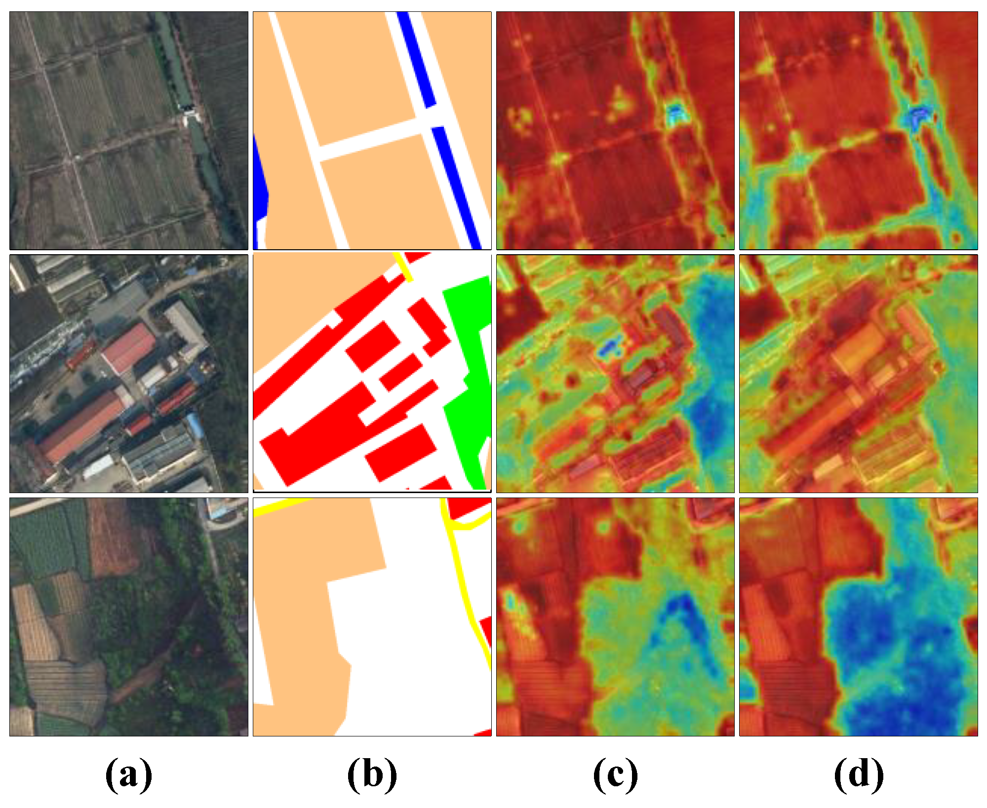
To address these issues, we propose a three-stage weakly supervised semantic segmentation framework that assigns different roles to CLIP, DINOv2, and SAM according to their complementary capabilities. In Stage 1, a lightweight adapter and a sigmoid-based multi-label decoupled distillation mechanism are introduced to align CLIP’s cross-modal priors with remote-sensing-specific semantics. By replacing Softmax-based class-competitive distillation with independent class-wise response optimization, this stage alleviates inter-class probability competition and produces more complete initial CAMs, as illustrated in Figure 1. In Stage 2, a DINOv2-guided Semantic Decomposition (DSD) module and a Spatial–Semantic Constraint (SSC) module are designed for semantically guided pseudo-label refinement. DSD decomposes large, merged connected regions before generating SAM prompts, while SSC constructs probability-guided point-and-box prompts and filters SAM outputs to reduce over-segmentation and semantic drift. In Stage 3, a compact segmentation network is warm-started with the weights learned in Stage 1 and retrained using the refined pseudo-labels, thereby eliminating the need for foundation models during inference.

The main contributions of this paper are summarized as follows:

• We develop a three-stage WSSS framework that assigns complementary roles to CLIP, DINOv2, and SAM for semantic transfer, region decomposition, and boundary refinement, respectively. The resulting pseudo-labels are used to train a compact segmentation network without foundation models at inference.
• We introduce a CLIP-based lightweight adapter with sigmoid-based multi-label decoupled distillation. This design converts the conventional class-competitive constraint into independent category-wise response optimization, thereby alleviating inter-class probability competition in densely coexisting remote sensing scenes and producing more complete initial CAMs.
• We design a DINOv2-assisted and SAM-assisted semantic-guided pseudo-label refinement strategy. The DINOv2-guided Semantic Decomposition (DSD) module decouples adhered large-scale connected regions before SAM prompting, while the Spatial–Semantic Constraint (SSC) module constructs probability-guided point-box prompts and filters SAM-generated masks to suppress area inflation and semantic drift, producing refined pseudo-labels with improved boundary quality and class attribution.

2. Related Work

2.1. Weakly Supervised Semantic Segmentation in Remote Sensing

Semantic segmentation is widely used in remote sensing applications such as land-cover mapping, building extraction, and environmental monitoring. Early fully supervised approaches were largely based on general-purpose segmentation architectures. Long et al. [18] introduced the fully convolutional network (FCN), which replaces fully connected layers with convolutional operations to enable end-to-end dense prediction. Ronneberger et al. [19] proposed U-Net, whose encoder–decoder structure and skip connections preserve spatial details during feature reconstruction. With the development of vision Transformers [5], Transformer-based architectures have become increasingly prominent in dense prediction. SegFormer [20], for example, combines a hierarchical Transformer encoder with a lightweight MLP decoder. Remote-sensing-specific studies have further explored global adaptive second-order representations [21], multi-branch prior information encoding for building segmentation [22], and sparse-token Transformers for building extraction [23]. Despite their strong performance, these methods depend on dense pixel-level annotations, which are expensive to acquire for large-scale remote sensing imagery.

Weakly supervised semantic segmentation (WSSS) reduces this annotation burden by learning pixel-level predictions using weaker forms of supervision, among which image-level labels are particularly cost effective and scalable [9,24]. Most image-level WSSS methods first generate class activation maps (CAMs) [7,8], convert them into pseudo-labels, and then train a segmentation network using the generated pixel-level supervision [9,10]. However, classification networks tend to respond primarily to the most discriminative regions of each class, resulting in incomplete spatial coverage and imprecise boundaries.

Recent WSSS methods have incorporated Transformer-based feature representations, contrastive learning, and region-level refinement to improve CAM quality. CTFA [6], for example, employs token-level and class-token contrastive learning [25] to alleviate feature over-smoothing and improve target localization. Other representative methods, including MoRe [26] and PCRE [27], further enhance feature representations and pseudo-label quality through feature- and region-level constraints. Despite these advances, achieving reliable WSSS in remote sensing imagery remains challenging. Remote sensing scenes commonly contain large homogeneous land-cover regions, substantial scale variation, weak foreground–background contrast, and multiple semantically similar classes within the same image. Consequently, CAMs often exhibit incomplete activation within large regions, as well as cross-class activation leakage and boundary adhesion between adjacent land-cover regions, all of which substantially reduce the reliability of the resulting pseudo-labels.

2.2. Vision Foundation Models in Remote Sensing

Vision foundation models provide complementary semantic and spatial priors for weakly supervised semantic segmentation. Contrastive Language–Image Pre-training (CLIP) [13] maps images and natural-language descriptions into a shared embedding space, enabling category-level semantic transfer without dense annotations. DINOv2 [14] learns semantically structured visual features through large-scale self-supervised pretraining and provides patch-level representations suitable for dense visual analysis. The Segment Anything Model (SAM) [15] supports prompt-based zero-shot mask generation and can generate masks with detailed object boundaries when supplied with appropriate point or box prompts.

Several studies have incorporated these models into weakly supervised semantic segmentation and remote sensing image segmentation. CLIMS [28] employs CLIP-based image–text matching and background suppression to improve the spatial coverage of CAMs. CLIP-ES [29] further exploits CLIP’s semantic prior throughout the WSSS pipeline to generate segmentation cues with reduced refinement overhead. WeCLIP+ [30] also demonstrates the value of transferring vision–language knowledge to weakly supervised segmentation. However, because CLIP is primarily pretrained on natural images, its visual representations may not transfer directly to the distinct overhead viewpoint, spatial organization, and land-cover semantics of remote sensing imagery.

SAM has also been adapted to remote sensing tasks. SAM-Adapter [31] introduces lightweight adapters to inject task-specific information into the frozen SAM architecture, while SAMRS [32] uses SAM to construct large-scale remote sensing segmentation data. RSPrompter [33] learns task-specific prompts for remote sensing instance segmentation, and RSRefSeg [34] extends foundation-model prompting to referring remote sensing image segmentation. Although these methods mainly address instance-level or referring segmentation rather than image-level WSSS, they demonstrate the effectiveness of task-specific prompting when transferring foundation models to remote sensing imagery. Recent foundation-model-assisted WSSS studies have explored both multi-stage seed refinement and training-time knowledge transfer. FMA-WSSS [35] employs a frozen CLIP model with learnable task-specific prompts and a SAM-based seeding module to progressively generate coarse-to-fine segmentation seeds, which subsequently serve as pseudo-labels for training a segmentation network. In another direction, From SAM to CAMs (S2C) [36] transfers SAM knowledge to the classifier during training through segment-level contrastive learning and confidence-aware supervision derived from CAM-prompted SAM masks, thereby improving CAM quality. More recently, ATSG [37] selects intermediate ViT features through adaptive token linking and employs SAM-guided post-processing to refine segmentation boundaries.

Despite this progress, effectively integrating foundation models into remote sensing WSSS remains challenging. Although recent studies improve segmentation seeds or transfer SAM knowledge to CAM generation, their application to complex remote sensing scenes still faces challenges arising from inter-class response competition, the adhesion of adjacent semantic regions, and unreliable SAM-generated masks. CLIP mainly provides image-level semantic knowledge and cannot independently guarantee spatially complete activation. SAM is class agnostic and sensitive to the quality of its prompts; coarse boxes obtained from raw CAMs may contain multiple adjacent categories or large amounts of background, causing mask expansion, category confusion, or prompt failure [17]. DINOv2 provides informative patch-level representations, but these features must be integrated with explicit class and spatial constraints to support reliable pseudo-label generation.

The proposed framework addresses these limitations by assigning complementary roles to the three foundation models. CLIP supplies cross-modal category priors through decoupled distillation, DINOv2 decomposes large adhered regions before prompting, and SAM refines their spatial boundaries under probability-guided point–box prompts and semantic consistency constraints. The refined pseudo-labels are subsequently used to warm-start and retrain a compact segmentation network, allowing the final model to operate independently of CLIP, DINOv2, and SAM during inference.

2.3. Cross-Modal Alignment and Knowledge Distillation

Knowledge distillation transfers representations or prediction distributions from a high-capacity teacher model to a smaller student network [38]. It has been widely studied in model compression, weakly supervised learning [39,40], and cross-modal knowledge transfer. With the development of vision–language models, CLIP-derived similarity scores have increasingly been used as semantic supervision for dense prediction. Such supervision can associate visual regions with category descriptions and improve the semantic coverage of CAMs [28,41].

Conventional knowledge distillation commonly applies softmax normalization followed by Kullback–Leibler (KL) divergence [38,42]. This formulation is appropriate when the target classes are mutually exclusive at the image level. Remote sensing WSSS, however, is inherently a multi-label problem: a single image patch may simultaneously contain buildings, roads, vegetation, water, and other land-cover categories [43]. Softmax normalization couples the responses of all classes, such that increasing the probability of one category necessarily suppresses the probabilities of the others. This inter-class competition is inconsistent with the co-occurrence patterns of remote sensing scenes and may weaken the responses of small or visually similar categories.

Multi-label learning instead estimates the probability of each category being present independently using a sigmoid activation [29,44]. Motivated by this distinction, the proposed method replaces softmax–KL distillation with sigmoid-based binary cross-entropy distillation. The resulting objective transfers CLIP’s category-level semantic knowledge without imposing artificial competition among co-occurring land-cover classes. A lightweight residual adapter is further introduced into the frozen CLIP visual branch to reduce the domain gap between natural-image and remote-sensing domains. Together, lightweight domain adaptation and multi-label decoupled distillation provide more reliable semantic responses for the subsequent pseudo-label refinement stage.

3. Methods

3.1. Overall Architecture

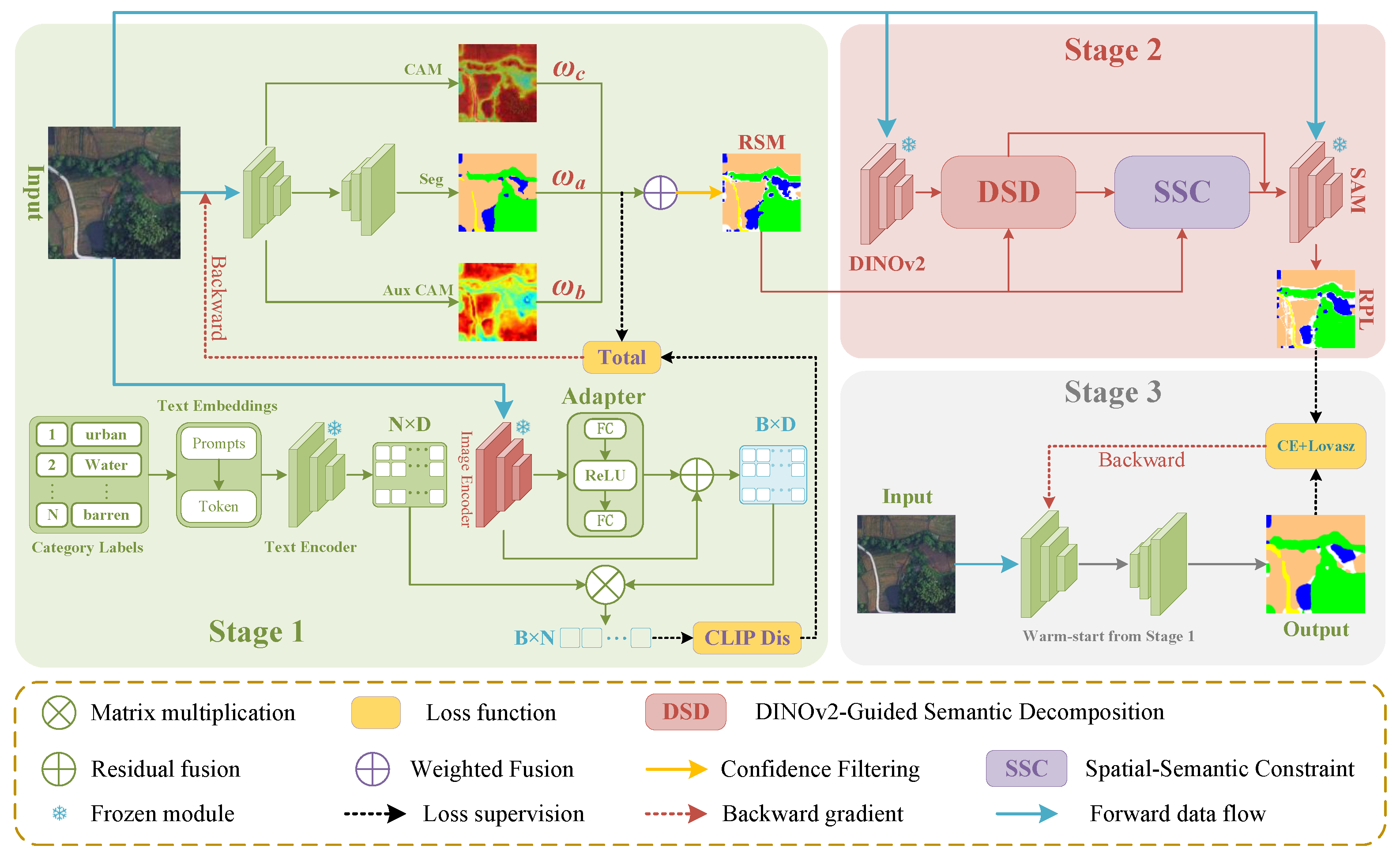
To overcome the limitations of coarse CAM localization and unreliable pseudo-label generation in remote sensing WSSS, we propose a three-stage framework based on decoupled cross-modal distillation and semantically guided pseudo-label refinement. The overall architecture is illustrated in Figure 2. The framework consists of three sequential stages. In the first stage, a CLIP-based cross-modal semantic alignment scheme is introduced: a learnable residual adapter is appended to the CLIP visual encoder, and a multi-label decoupled distillation strategy is employed to align the backbone’s classification responses with the semantic priors acquired by CLIP from large-scale image–text pairs. This design mitigates overly localized CAM activations and inter-class competition arising from dense class co-occurrence in remote sensing imagery. In the second stage, the segmentation probability map, primary CAM, and auxiliary CAM produced by the Stage-1 model are fused to form a Reliable Seed Mask (RSM). A DINOv2-guided Semantic Decomposition (DSD) module and a Spatial–Semantic Constraint (SSC) module are then used to guide SAM-based refinement by decomposing large merged regions, constructing reliable prompts, and filtering excessively expanded or semantically inconsistent masks. This stage produces refined pseudo-labels with sharp boundaries and consistent class assignments. In the third stage, a compact end-to-end segmentation network is warm-started with the weights learned in Stage 1 and subsequently retrained using the refined pseudo-labels. This initialization accelerates convergence and allows the network to retain the cross-modal semantic knowledge distilled from CLIP, enabling accurate remote sensing segmentation without relying on foundation models during inference.

3.2. CLIP-Based Decoupled Cross-Modal Distillation (Stage 1)

Under weak supervision with only image-level labels, conventional classification-based methods tend to generate spatially incomplete class activation maps (CAMs), because the classification objective usually encourages the network to focus on only the most discriminative regions of target objects. To alleviate this localization bias, we introduce CLIP as a cross-modal teacher to regularize and refine the classification responses of the backbone. However, CLIP is pretrained predominantly on generic web-scale image-text pairs rather than specialized remote sensing imagery, resulting in a considerable domain gap when it is directly applied to remote sensing scenes. To retain the zero-shot generalization ability of CLIP while adapting its representations to remote-sensing-specific semantics, we design a remote-sensing-oriented prompt ensemble and a lightweight visual adaptation mechanism.

To preserve the generalizable knowledge encoded in CLIP, both its visual and textual encoders remain frozen throughout training. On the textual branch, we construct a remote-sensing-oriented prompt ensemble for each target class. Specifically, the ensemble comprises five fixed templates: “a satellite image of [class]”, “aerial view of [class]”, “a top-down view of [class] area”, “satellite photo showing [class]”, and “a remote sensing image of [class]”. The same five templates are shared across all three datasets, whereas [class] is replaced with the dataset-specific semantic category name. Thus, each dataset has its own set of class-level text representations according to its category definitions. Only the semantic categories involved in training and evaluation are included in prompt construction. For each category, the resulting five text embeddings are individually L2-normalized, averaged, and normalized again to form the final class-level representation. By incorporating alternative descriptions of overhead imagery, the ensemble reduces dependence on any single prompt expression and provides a more stable textual representation for each remote-sensing category.

On the visual branch, a residual adapter controlled by a learnable scaling coefficient is appended to the frozen CLIP visual encoder. By updating only the lightweight adapter and its scaling coefficient, the proposed design adapts the generic CLIP representation space to the remote sensing domain while reducing the risk of catastrophic forgetting that may arise from full-parameter fine-tuning. Given an original visual feature $f_v$ extracted by the CLIP visual encoder, the adapted feature is computed as

$$f_v^{\prime }=\mathrm{Norm}\left(f_v+\alpha ·\mathrm{Adapter}\left(f_v\right)\right)$$

(1)

where $\mathrm{Adapter}(·)$ denotes a lightweight multilayer perceptron consisting of two fully connected layers and a ReLU activation function. The learnable scalar $\alpha$ controls the strength of the residual domain adaptation and is jointly optimized with the adapter parameters. The operator $\mathrm{Norm}(·)$ denotes L2 normalization along the feature dimension. The adapted image feature $f_v^{\prime }$ is then compared with the normalized textual embeddings of all classes through dot-product similarity. The resulting similarities are multiplied by a fixed logit scaling factor of 100 to produce the multi-label classification logits of the CLIP branch.

The adapter and the scaling coefficient $\alpha$ are optimized using an image-level multi-label soft-margin loss ${\mathcal{L}}_{\mathrm{clip}}$ to capture remote-sensing-specific semantics. The resulting class predictions are subsequently employed as soft supervision for the student backbone. Within the backbone, hierarchical features extracted by the Transformer encoder are processed by primary and auxiliary $1\times 1$ classifiers. Their corresponding CAMs are generated by applying the learned classifier weights to the feature maps without introducing additional learnable parameters.

Remote sensing scenes commonly contain multiple coexisting land-cover categories. However, conventional Softmax-based KL-divergence distillation forces the class probabilities to sum to one, thereby introducing artificial competition among different categories. A high probability assigned to one class may consequently suppress the responses of other coexisting classes. To address this limitation, we propose a sigmoid-based decoupled distillation mechanism that decomposes multi-class supervision into C independent binary distillation problems. Under this formulation, the probability of each category is estimated independently, avoiding mutual suppression among coexisting categories.

Let $s_c$ and $t_c$ denote the logits produced by the student backbone and the domain-adapted CLIP teacher for the c-th class, respectively. The teacher soft targets are computed as

$$q_c=\sigma \left({\displaystyle \frac{t_c}{T}}\right)$$

(2)

where $q_c$ denotes the soft target provided by the CLIP teacher, and $T=2.0$ is the temperature hyperparameter shared by the teacher and student branches during distillation. It controls the smoothness of the teacher soft targets and the corresponding temperature-scaled student predictions. During distillation, $q_c$ is detached from the computation graph and treated as a fixed supervisory target. Consequently, ${\mathcal{L}}_{\mathrm{clip}}$ optimizes the visual adapter and the scaling coefficient $\alpha$, whereas ${\mathcal{L}}_{\mathrm{distill}}$ updates only the student backbone. Therefore, the gradients of the distillation loss are propagated only through the student branch. The decoupled distillation loss is formulated as

$${\mathcal{L}}_{\mathrm{distill}}={\displaystyle \frac{T^2}{C}}{\displaystyle \sum _{c=1}^C}{\mathcal{L}}_{\mathrm{BCE}}\left({\displaystyle \frac{s_c}{T}},q_c\right)$$

(3)

where ${\mathcal{L}}_{\mathrm{BCE}}$ denotes the binary cross-entropy with logits loss, and C denotes the number of target classes. Following common temperature-scaled distillation practice, the factor $T^2$ is introduced to balance the gradient magnitude.

The overall training objective of Stage 1 integrates multiple complementary supervision signals:

$$\begin{array}{cc}\hfill {\mathcal{L}}_{\mathrm{total}}& ={\mathcal{L}}_{\mathrm{cls}}+{\mathcal{L}}_{\mathrm{cls}}^{\mathrm{aux}}+{\lambda }_{\mathrm{ptc}}{\mathcal{L}}_{\mathrm{ptc}}+{\lambda }_{\mathrm{ctc}}{\mathcal{L}}_{\mathrm{ctc}}+{\lambda }_{\mathrm{clip}}{\mathcal{L}}_{\mathrm{clip}}\hfill \\ \hfill & + {\omega }_{\mathrm{d}}\left(i\right){\lambda }_{\mathrm{distill}}{\mathcal{L}}_{\mathrm{distill}}\hfill \\ \hfill & + {\omega }_{\mathrm{s}}\left(i\right)\left({\lambda }_{\mathrm{seg}}{\mathcal{L}}_{\mathrm{seg}}+{\lambda }_{\mathrm{reg}}{\mathcal{L}}_{\mathrm{reg}}+{\lambda }_{\mathrm{joi}}{\mathcal{L}}_{\mathrm{joi}}\right)\hfill \end{array}$$

(4)

where ${\mathcal{L}}_{\mathrm{cls}}$ and ${\mathcal{L}}_{\mathrm{cls}}^{\mathrm{aux}}$ denote the primary and auxiliary multi-label classification losses, respectively. The losses ${\mathcal{L}}_{\mathrm{ptc}}$ and ${\mathcal{L}}_{\mathrm{ctc}}$ regularize feature consistency at the patch-token and class-token levels. The segmentation loss ${\mathcal{L}}_{\mathrm{seg}}$ is computed using pseudo-labels generated from the fused CAMs, while ${\mathcal{L}}_{\mathrm{reg}}$ denotes the dense energy regularization loss used to improve object-boundary alignment. ${\mathcal{L}}_{\mathrm{joi}}$ promotes consistency between the outputs of the primary and foreground decoder branches. The effects of the two CLIP-related loss weights introduced in this work are quantitatively evaluated on the LoveDA dataset, as reported in the subsequent ablation study.Based on this comparison, ${\lambda }_{\mathrm{clip}}=0.2$ and ${\lambda }_{\mathrm{distill}}=0.5$ are selected as the default settings for all experiments. It should be emphasized that ${\omega }_{\mathrm{d}}\left(i\right)$ and ${\omega }_{\mathrm{s}}\left(i\right)$ are binary scheduling gates rather than tunable loss weights, and their values are restricted to either 0 or 1. Specifically, ${\omega }_{\mathrm{d}}\left(i\right)=0$ for $i<1500$ and ${\omega }_{\mathrm{d}}\left(i\right)=1$ for $i\ge 1500$, thereby postponing cross-modal distillation until the adapter has learned an effective domain mapping. Similarly, ${\omega }_{\mathrm{s}}\left(i\right)=0$ for $i<2000$ and ${\omega }_{\mathrm{s}}\left(i\right)=1$ for $i\ge 2000$, delaying the segmentation-related objectives until the CAM-derived pseudo-labels become sufficiently reliable.

Through the proposed decoupled cross-modal distillation mechanism, the domain-adapted CLIP teacher provides independent class-wise semantic supervision for the student backbone. This formulation avoids the artificial inter-class competition introduced by Softmax-based distillation and is more compatible with multi-label remote sensing scenes. The transferred semantic supervision helps the student generate more comprehensive class responses, thereby improving the spatial coverage and structural completeness of the initial CAMs. These CAMs subsequently provide more reliable localization cues for pseudo-label refinement.

3.3. Semantic-Guided Pseudo-Label Refinement (Stage 2)

After the cross-modal semantic alignment in the first stage, the regional completeness of initial CAMs is substantially improved. However, due to the low spatial resolution of deep classification features, the resulting activation regions remain coarse along physical boundaries and cannot be directly used as pixel-level supervision. To obtain reliable pseudo-labels, SAM is used as a mask generator under semantic and spatial constraints rather than as a standalone boundary refinement module. Nevertheless, applying SAM to remote sensing scenes poses two key challenges. First, SAM heavily relies on clear low-level image edges, rendering it prone to merging multiple distinct semantic instances into a single target when confronted with large, contiguous, and geometrically irregular land covers. Second, directly using coarse CAMs as SAM prompts introduces substantial background noise and induces conflicts between predicted masks and semantic categories.

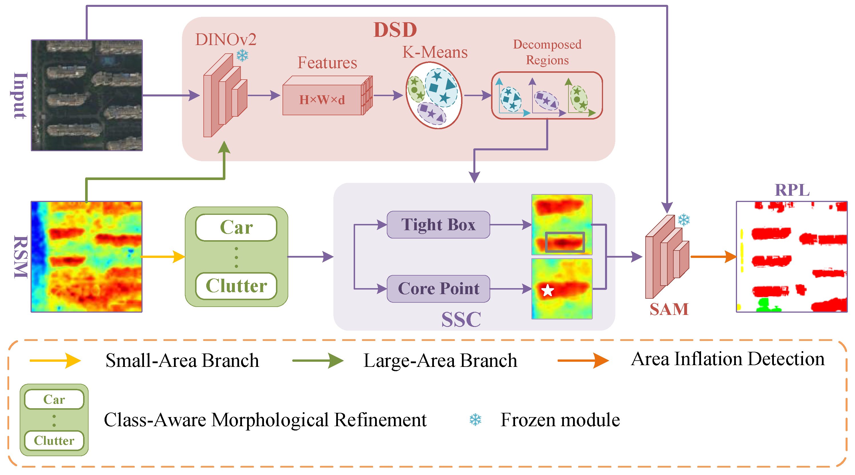
To address these challenges, a reliable seed label is first constructed, after which a DINOv2-guided Semantic Decomposition (DSD) module and a Spatial–Semantic Constraint (SSC) module are jointly designed to guide SAM toward accurate segmentation. The overall pipeline is illustrated in Figure 3.

3.3.1. Multi-Branch Probability Fusion and Confidence Filtering

To obtain a seed label more robust than a single CAM, the multi-branch probability outputs of the Stage-1 model are fully exploited. Given an input image $I\in {\mathbb{R}}^{3\times H\times W}$, the segmentation decoder and the dual classification heads of the Stage-1 network respectively produce three probability tensors: the segmentation probability map $P^{\mathrm{seg}}\in {\mathbb{R}}^{C\times H\times W}$, the primary class activation map $P^{\mathrm{cam}}\in {\mathbb{R}}^{C\times H\times W}$, and the auxiliary class activation map $P^{\mathrm{aux}}\in {\mathbb{R}}^{C\times H\times W}$, where C denotes the total number of classes, and $H\times W$ denotes the spatial resolution. These three probability tensors are combined element-wise using predefined weights:

$$\widehat{P}=w_a·P^{\mathrm{seg}}+w_b·P^{\mathrm{aux}}+w_c·P^{\mathrm{cam}}$$

(5)

where $\widehat{P}$ denotes the fused multi-view probability tensor, and $w_a=0.7$, $w_b=0.15$, and $w_c=0.15$ are the corresponding fusion weights. The fusion coefficients satisfy $w_a,w_b,w_c\ge 0$ and $w_a+w_b+w_c=1$. Since the segmentation decoder provides dense pixel-level predictions, it is assigned a dominant weight in the fusion. In contrast, the primary and auxiliary CAMs provide complementary but spatially coarser localization cues. The two CAM branches are assigned equal weights because they play the same auxiliary role in seed generation. An ablation study was conducted to compare and validate multiple representative weight configurations, as presented in the subsequent experimental analysis. The experimental results demonstrate that $(w_a,w_b,w_c)=(0.70, 0.15, 0.15)$ provides the best overall performance and is therefore selected as the final weight configuration. Subsequently, a per-pixel preliminary class map is obtained by applying $\arg \max$ along the channel dimension:

$$M_{\mathrm{rough}}(i,j)=\arg \underset{c\in \{0,1,\dots ,C-1\}}{\max }\widehat{P}(c,i,j)$$

(6)

To filter out pixels with insufficient prediction confidence, a confidence threshold $\tau$ is applied as a secondary screening at each pixel location:

$$M_{\mathrm{rough}}(i,j)=\left\{\begin{array}{cc}{M}_{\mathrm{rough}}(i,j),\hfill & \mathrm{if}{\max }_c\widehat{P}(c,i,j)\ge \tau \hfill \\ 255,\hfill & \mathrm{otherwise}\hfill \end{array}\right.$$

(7)

where the threshold is empirically set to $\tau =0.55$. The resulting map is the Reliable Seed Mask (RSM), which serves as the unified input to the subsequent DSD and SSC modules. This step elevates the quality of the SAM input seeds from that of a single CAM to that of a high-confidence view dominated by the segmentation probability, providing the foundation for the SAM-based pseudo-label refinement.

3.3.2. DINOv2-Guided Semantic Decomposition (DSD)

While the RSM exhibits relatively high class confidence, it often presents a particular failure mode on large homogeneous categories such as water bodies, farmland, forests, and barren land: due to the limited resolution of CAMs and the homogeneity of classification responses, multiple spatially adjacent but physically independent land-cover instances are erroneously merged into a single connected region. If such a region is directly fed into SAM as a prompt, SAM generates a single mask along its bounding box, lumping multiple independent objects into one output and consequently losing the instance boundaries.

To address this issue, a DINOv2-guided Semantic Decomposition (DSD) module is proposed, which performs semantic decoupling on adhered connected regions using high-dimensional semantic features before they enter SAM. Through self-supervised pretraining, DINOv2 exhibits notable intra-class compactness in its deep feature space: pixel feature vectors belonging to the same semantic class spontaneously form compact clusters on the manifold, while different instances, even within the same class, retain distinguishable differences in feature distribution. This property effectively compensates for SAM’s limitation of relying solely on low-level visual edges.

Specifically, given an input image, DINOv2 first extracts a pixel-level feature map $F\in {\mathbb{R}}^{H\times W\times d}$, where H, W, and d denote its height, width, and feature dimension, respectively. For each target large-scale category c, a class-specific binary candidate mask $M_c$ is extracted from the RSM, and its area $A_c$ is calculated as the number of foreground pixels. Semantic decomposition is activated when $A_c\ge A_{\min }$; otherwise, the candidate mask is retained without decomposition to avoid unnecessary fragmentation. For each activated candidate mask, the corresponding DINOv2 features are clustered using K-Means. The cluster number K controls the decomposition granularity and is determined by a predefined dataset- and area-dependent rule as detailed in the implementation settings. The objective function is defined as

$$\underset{\{C_1,\dots ,C_K\}}{\min }{\displaystyle \sum _{k=1}^K}\sum _{F_i\in C_k}{∥F_i-{\mu }_k∥}_2^2$$

(8)

where $C_k$ denotes the k-th semantic cluster, ${\mu }_k$ denotes its feature centroid, and ${\parallel ·\parallel }_2$ denotes the Euclidean norm. By exploiting the semantic consistency of DINOv2 features, DSD decomposes a spatially merged candidate mask into finer semantic clusters. Connected-component analysis is then applied to each cluster mask to obtain spatially separated sub-regions for SAM prompting, thereby reducing the risk of merging adjacent land-cover regions into a single mask.

3.3.3. Spatial–Semantic Constraint Module (SSC)

After DSD-based decomposition, the resulting sub-regions are represented as binary masks and therefore cannot be directly used as prompts for SAM. Moreover, although SAM can generate high-quality masks in a class-agnostic manner, it lacks explicit mechanisms for preventing mask over-expansion, inter-instance confusion, and semantic conflicts with existing predictions. The SSC module therefore performs two complementary functions: it converts the sub-regions into reliable geometric prompts for SAM and applies geometric and semantic constraints to SAM’s raw outputs, thereby improving the stability and semantic consistency of the final pseudo-labels in scenes containing multiple co-occurring classes.

For each candidate region R supplied to SAM, where R is either a DSD-derived sub-region or the original connected region when DSD is not activated, SSC constructs a point prompt and a box prompt for SAM. The box prompt is defined as the tight bounding box of R without outward padding, thereby avoiding the inclusion of semantically irrelevant background areas. The positive point prompt is selected as the pixel with the highest confidence in the class-specific probability map:

$$p_R^{+}=\arg \underset{(i,j)\in R}{\max }{P}_c(i,j)$$

(9)

where $P_c$ denotes the probability map for class c obtained during RSM generation. Compared with using the geometric centroid, this probability-guided selection avoids cases in which the centroid of a connected region lies within a background hole or a boundary transition area, thereby placing the positive prompt in the high-confidence interior of the corresponding land-cover region. The point and box prompts provide complementary information: the box prompt conveys the approximate spatial extent of the candidate region, whereas the point prompt provides a reliable class-consistent foreground anchor. Their joint use reduces the boundary drift that may occur when SAM is guided solely by a box prompt.

When SAM processes adjacent regions with similar textures, it may expand toward the boundaries of the prompt box and produce a mask substantially larger than the corresponding candidate region. To address this issue, we introduce an area-ratio constraint. Specifically, given a SAM-generated mask $M_{\mathrm{SAM}}$ and its corresponding candidate region R, the predicted mask is identified as over-segmented and discarded if

$${\displaystyle \frac{\left|M_{\mathrm{SAM}}\right|}{\left|R\right|}}>\gamma ,$$

(10)

where $\left|M_{\mathrm{SAM}}\right|$ and $\left|R\right|$ denote the areas of the SAM-generated mask and its corresponding candidate region, respectively. If this condition is satisfied, the SAM prediction is rejected, and the corresponding candidate region is assigned the ignore index in the final pseudo-label to avoid introducing noisy supervision during training. Since the area ratio is dimensionless, the threshold $\gamma$ does not require explicit rescaling according to the ground sampling distance. We set $\gamma =4.0$ for all three datasets. This value permits moderate mask expansion to compensate for incomplete initial localization while suppressing severe over-expansion.

In remote sensing scenes containing multiple co-occurring classes, masks generated for different classes may overlap at the same pixel locations. Updating the pseudo-labels solely according to mask generation order could allow a subsequently processed class to overwrite an earlier high-confidence prediction, resulting in semantic inconsistency. To prevent this, SSC allows a SAM prediction to update only those RSM pixels that are assigned to the same semantic class as the current candidate region, the ignore label (255), or a designated background label, where applicable. Pixels carrying high-confidence predictions of other foreground classes are protected from being overwritten. This conflict-resolution rule implicitly uses the confidence-filtered RSM to preserve reliable foreground predictions while allowing ignored and eligible background regions to be refined by SAM. Consequently, it prevents SAM masks from incorrectly encroaching upon regions belonging to other classes because of visual similarity.

By combining DSD-based semantic decomposition with SSC-based prompt construction, area-ratio constraint, and conflict-aware label updating, the framework ultimately produces refined pseudo-labels (RPLs) with accurate boundaries and reliable semantic assignments. These pseudo-labels provide high-quality pixel-level supervision for the end-to-end segmentation network in Stage 3.

3.4. Warm-Start Retraining (Stage 3)

Although the cascade framework based on multiple vision foundation models achieves remarkable performance in the pseudo-label generation stage, the substantial parameter count and high inference latency of CLIP and SAM make it impractical to directly deploy them in real-world remote sensing observation tasks. At the same time, the high-quality pseudo-labels generated in Stage 2 provide a strong basis for further improving the performance of weakly supervised models. To this end, a warm-start retraining stage is designed, in which an efficient feed-forward fully convolutional segmentation network is trained under the supervision of the refined pseudo-labels to enable end-to-end high-accuracy inference.

Specifically, rather than reinitializing the final segmentation network from generic ImageNet-pretrained weights, we initialize it using the backbone weights learned in Stage 1; instead, the backbone weights optimized by decoupled distillation in Stage 1 are loaded as a warm start. At inference, only the compact segmentation network is retained, avoiding the computational overhead of CLIP, DINOv2, and SAM. In terms of supervision design, although the pseudo-labels have been refined by DSD and SSC, residual noise may still exist in boundary transition zones. A cross-entropy loss with label smoothing is therefore adopted to implicitly regularize the noisy labels and to alleviate overfitting to incorrect supervision. Furthermore, the standard cross-entropy loss is sensitive to the class imbalance commonly observed in remote sensing land covers, and the independence of pixel-wise losses makes it difficult to constrain the overall geometric shape of segmented regions. To address these limitations, the Lovász-Softmax loss is introduced alongside the cross-entropy loss. Let p denote the prediction probability map produced by the network and y denote the corresponding refined pseudo-label map; the joint training objective in the retraining stage is defined as

$$\mathcal{L}={\mathcal{L}}_{\mathrm{CE}}(p,y)+{\lambda }_{\mathrm{lov}}\left(t\right)·{\mathcal{L}}_{\mathrm{Lovasz}}(p,y)$$

(11)

where t denotes the training epoch and ${\lambda }_{\mathrm{lov}}\left(t\right)$ is an epoch-dependent weight for the Lovász-Softmax loss, defined as

$${\lambda }_{\mathrm{lov}}\left(t\right)=\left\{\begin{array}{cc}0,\hfill & t<2\hfill \\ 0.5,\hfill & t\ge 2\hfill \end{array}\right.$$

(12)

The two losses serve complementary roles: the cross-entropy loss ensures the accuracy of local pixel-wise classification, while the Lovász-Softmax loss directly optimizes the per-class IoU metric, enhancing the model’s ability to fit complex land-cover boundaries at the regional level. This combination is particularly effective in class-imbalanced scenarios.

Through warm-start initialization combined with joint loss optimization, the deployed segmentation network is fully decoupled from the inference of any large foundation model. This substantially narrows the performance gap between weakly supervised and fully supervised segmentation models, enabling end-to-end, low-latency, high-accuracy remote sensing image segmentation.

4. Experiments

4.1. Datasets and Implementation Details

To comprehensively validate the effectiveness of the proposed method, extensive experiments are conducted on three mainstream remote sensing semantic segmentation datasets: Potsdam [45], DeepGlobe [46], and LoveDA [1]. These benchmarks cover urban aerial, urban–rural composite, and global land-cover scenarios, respectively, providing a comprehensive evaluation of the proposed framework under diverse imaging conditions.

The Potsdam dataset is one of the aerial remote sensing segmentation benchmarks provided by ISPRS, captured over the city of Potsdam, Germany. It contains 38 orthorectified aerial images, each with a resolution of 6000 × 6000 pixels and a spatial resolution of 0.05 m. The dataset is annotated with six semantic categories: impervious surface, building, low vegetation, tree, car, and clutter. For training, the original images are cropped into non-overlapping patches of 512 × 512 pixels, yielding 4477 patches in total, which are further split into 2783 training samples and 1694 test samples.

The LoveDA dataset consists of high-resolution urban–rural remote sensing images collected from three Chinese cities, namely Nanjing, Changzhou, and Wuhan, comprising 5987 original images with a resolution of 1024 × 1024 pixels and a spatial resolution of 0.3 m. It covers both urban and rural scenarios and is annotated with seven semantic categories: building, road, water, barren, forest, agriculture, and background. The original images are cropped into non-overlapping patches of 512 × 512 pixels, yielding 16,764 patches in total, which are split into 11,732 training, 2512 validation, and 2520 test samples.

The DeepGlobe dataset is distinguished by its absence of clearly separable foreground and background categories [47], being primarily designed for large-area land-cover classification rather than precise small-object segmentation. It contains 803 high-resolution remote sensing images, each with a resolution of 2448 × 2448 pixels and a spatial resolution of 0.5 m. The dataset provides annotations for seven categories: urban, agriculture, rangeland, forest, water, barren, and unknown. According to the official evaluation protocol, the unknown class is excluded during both training and evaluation, leaving six effective semantic categories in practice. The original images are cropped into non-overlapping patches of 512 × 512 pixels, yielding 13,275 patches in total, which are split into 9100 training, 2150 validation, and 2025 test samples.

The proposed framework consists of three stages, each adopting its own optimization or inference configuration. In Stage 1, the AdamW optimizer is employed with a weight decay of 1 × ${10}^{-2}$; the initial learning rate is set to 4 × ${10}^{-5}$ on Potsdam and 2 × ${10}^{-5}$ on LoveDA and DeepGlobe, with a batch size of 8 and a total of 20,000 training iterations. During inference, CAMs are generated at multi-scale ratios of (1.0, 0.5, 1.5) and fused by averaging, followed by post-processing refinement with a fully connected CRF [48]. Stage 2 is a feed-forward inference process that requires no training, with pseudo-labels generated according to the predefined rules of the DSD and SSC modules. SAM with the ViT-H backbone is consistently used in the primary experiments on Potsdam, LoveDA, and DeepGlobe. In the DSD module, $A_c$ denotes the area of the class-specific candidate mask $M_c$, measured by its number of foreground pixels. Semantic decomposition is activated when $A_c\ge A_{\min }$. The parameters $A_{\min }$ and K follow predefined scale- and complexity-aware criteria rather than being independently adjusted on the test sets. Specifically, $A_{\min }$ is used to prevent unstable decomposition of very small candidate masks. Since objects with the same physical extent occupy more pixels in imagery with finer spatial resolution, a larger pixel-area threshold is adopted for finer-resolution datasets. Accordingly, $A_{\min }$ is set to 400, 300, and 200 pixels for Potsdam, LoveDA, and DeepGlobe, whose spatial resolutions are 0.05, 0.3, and 0.5 m, respectively. For Potsdam and LoveDA, $K=2$ is adopted as the minimum nontrivial cluster number, enabling semantic decomposition while limiting unnecessary fragmentation. For DeepGlobe, a predefined area-aware clustering rule is used: $K=2$ when $A_c<5000$ and $K=3$ when $A_c\ge 5000$. The additional cluster for large DeepGlobe masks accommodates their greater spatial extent and potential appearance diversity. The cluster number is limited to three to avoid excessive fragmentation and computational overhead. These rules are determined before test evaluation and remain fixed throughout all experiments. Stage 3 is warm-started by loading the optimal weights from Stage 1 and optimized using SGD with an initial learning rate of 5 × ${10}^{-5}$, a momentum of 0.9, a weight decay of 1 × ${10}^{-4}$, a batch size of 8, and 20 training epochs.

All experiments are implemented in PyTorch 1.11.0 with Python 3.8 and conducted on a single NVIDIA RTX 4090 GPU running Ubuntu 20.04.

4.2. Evaluation Metrics

We evaluate segmentation performance using mean Intersection-over-Union (mIoU), Precision, Recall, F1 score, and overall accuracy (OA). The mIoU is used as the primary metric, while the remaining metrics provide complementary assessments of classification accuracy and class-wise performance. Let ${\mathrm{TP}}_i$, ${\mathrm{FP}}_i$, and ${\mathrm{FN}}_i$ denote the numbers of true-positive, false-positive, and false-negative pixels for class i, respectively, and let N denote the number of evaluated classes. The metrics are defined as follows:

$$\mathrm{mIoU}={\displaystyle \frac{1}{N}}{\displaystyle \sum _{i=1}^N}{\displaystyle \frac{{\mathrm{TP}}_i}{{\mathrm{TP}}_i+{\mathrm{FP}}_i+{\mathrm{FN}}_i}},$$

(13)

$$\mathrm{Precision}={\displaystyle \frac{1}{N}}{\displaystyle \sum _{i=1}^N}{\displaystyle \frac{{\mathrm{TP}}_i}{{\mathrm{TP}}_i+{\mathrm{FP}}_i}},$$

(14)

$$\mathrm{Recall}={\displaystyle \frac{1}{N}}{\displaystyle \sum _{i=1}^N}{\displaystyle \frac{{\mathrm{TP}}_i}{{\mathrm{TP}}_i+{\mathrm{FN}}_i}},$$

(15)

$$\mathrm{F}1={\displaystyle \frac{1}{N}}{\displaystyle \sum _{i=1}^N}{\displaystyle \frac{2{\mathrm{TP}}_i}{2{\mathrm{TP}}_i+{\mathrm{FP}}_i+{\mathrm{FN}}_i}},$$

(16)

$$\mathrm{OA}={\displaystyle \frac{{\sum }_{i=1}^N{\mathrm{TP}}_i}{{\sum }_{i=1}^N\left({\mathrm{TP}}_i+{\mathrm{FN}}_i\right)}}.$$

(17)

Precision, Recall, and F1 are computed for each class and then macro-averaged, preventing large-area categories from dominating the reported results. Dataset-provided unknown or ignore-label pixels are excluded from metric computation.

To quantitatively evaluate boundary delineation quality, we additionally adopt mean Boundary Intersection-over-Union (mBIoU) as a boundary-sensitive evaluation metric. For class i, let $P_i$ and $G_i$ denote the predicted and ground-truth regions, respectively, and let ${\mathcal{B}}_d(·)$ denote the boundary region extracted with a width of d. The class-wise Boundary IoU is defined as

$${\mathrm{BIoU}}_i={\displaystyle \frac{\left|{\mathcal{B}}_d\left(P_i\right)\cap {\mathcal{B}}_d\left(G_i\right)\right|}{\left|{\mathcal{B}}_d\left(P_i\right)\cup {\mathcal{B}}_d\left(G_i\right)\right|}}$$

(18)

The mean Boundary IoU is obtained by averaging the class-wise Boundary IoU values over the N evaluated semantic classes:

$$\mathrm{mBIoU}={\displaystyle \frac{1}{N}}{\displaystyle \sum _{i=1}^N}{\mathrm{BIoU}}_i$$

(19)

As with the other evaluation metrics, unknown or ignore-label pixels are excluded from the mBIoU calculation.

4.3. Comparison with State-of-the-Art Methods

To thoroughly validate the effectiveness of the proposed method, comprehensive comparisons are conducted on the Potsdam, LoveDA, and DeepGlobe datasets against representative state-of-the-art WSSS methods, including MoRe [26], CTFA [6], WeCLIP+ [30], PCRE [27], and ATSG [37]. These benchmarks span urban aerial, urban–rural composite, and global land-cover scenarios, collectively verifying the stability and cross-scene generalization capability of the proposed framework. In addition, comparisons with three representative fully supervised semantic segmentation methods, namely UNetFormer [49], PIDNet [50], and DeepKANSeg [51], are conducted on LoveDA and DeepGlobe to quantify the performance gap between image-level weak supervision and full supervision.

4.3.1. Results on the Potsdam Dataset

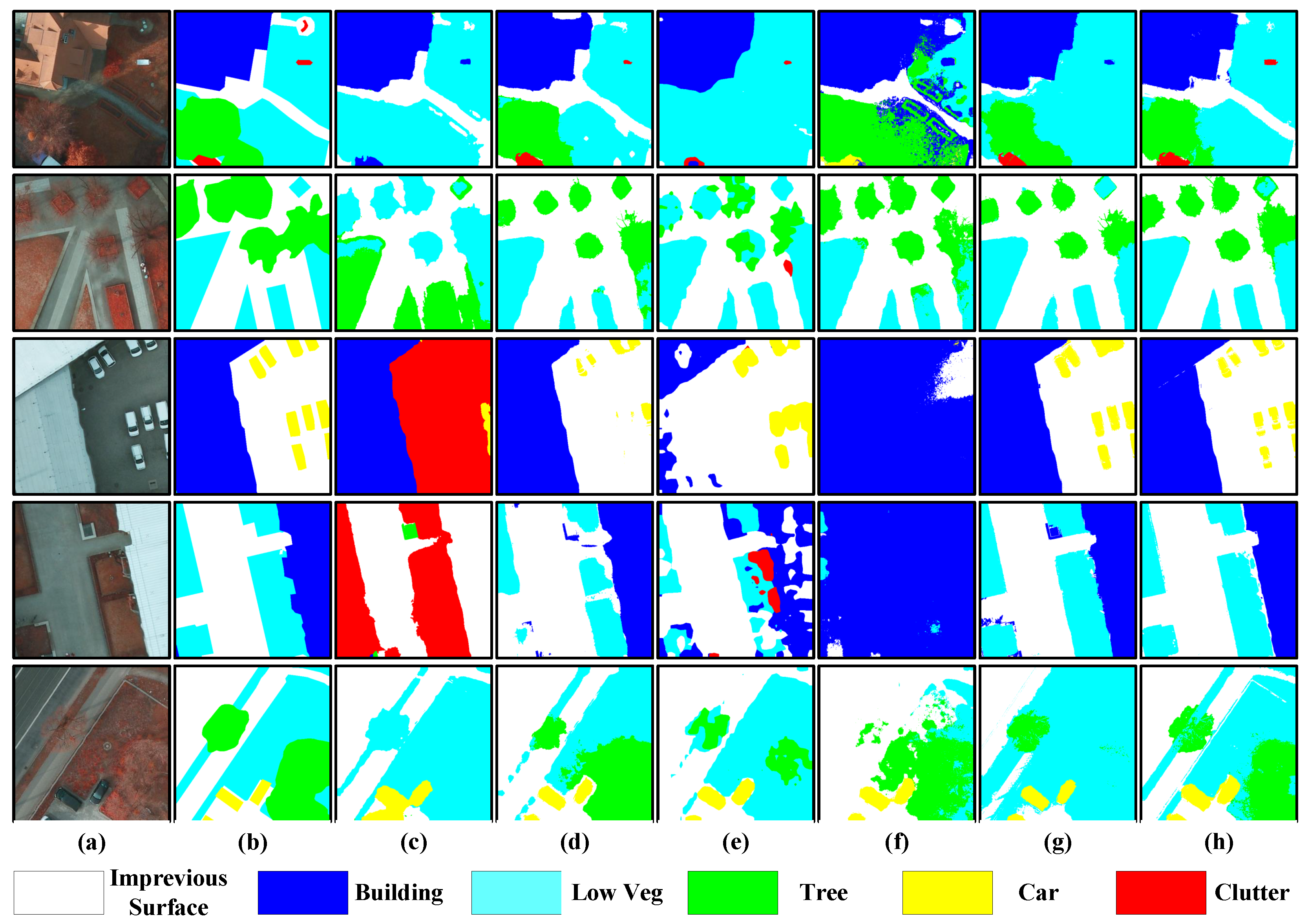
Both quantitative and qualitative comparisons are conducted on the Potsdam dataset, with the qualitative results illustrated in Figure 4 and the quantitative results summarized in

Table 1. Per-class and overall comparison with state-of-the-art WSSS methods on the Potsdam dataset, together with their total pipeline time. Bold values indicate the best result in each column. For total pipeline time, lower is better.

Method	Imp. Surface	Building	Low Veg	Tree	Car	Clutter	mIoU (%)	Time (min)
CTFA [6]	58.75	50.58	51.20	50.35	50.82	17.96	46.61	213
MoRe [26]	62.86	69.47	4.35	40.38	55.18	10.51	40.46	263
WeCLIP+ [30]	58.42	72.83	37.01	24.68	65.60	14.18	45.45	289
PCRE [27]	60.32	62.46	41.36	44.86	51.99	7.11	44.68	354
ATSG [37]	61.98	49.83	43.80	60.40	1.53	56.09	45.61	452
Ours	62.26	69.52	54.53	53.37	59.67	19.63	53.16	301

. As shown in Table 1, the proposed method outperforms the second-best method CTFA in terms of mIoU by 6.55 percentage points. Among the six semantic categories, the proposed method achieves the best performance on the Low Veg class with 54.53%, and consistently ranks among the top performers on Imp Surface, Building, Tree, and Car. It is worth noting that several baselines exhibit substantial inter-class imbalance: ATSG reaches 56.09% on Clutter but only 1.53% on Car, revealing a pronounced class-wise bias, while MoRe achieves a mere 4.35% on Low Veg, reflecting the fragility of baseline methods in multi-class coexisting scenarios. In contrast, the proposed method maintains stable and high responses across all six categories. This stability stems from two key designs: the CLIP-based multi-label decoupled distillation in Stage 1, which thoroughly releases inter-class probability competition, and the DSD and SSC modules in Stage 2, which enable precise decoupling of adhered land covers.

To further evaluate computational efficiency, we report the training time of all methods in the last column of Table 1. As shown in Table 1, the proposed framework requires 301 min, which is lower than the 354 min required by PCRE and the 452 min required by ATSG. Its training time is also comparable to the 289 min required by WeCLIP+, although it is higher than the 213 min required by CTFA and the 263 min required by MoRe. Despite not achieving the shortest training time, the proposed method obtains the highest mIoU of 53.16%, outperforming the second-best result by 6.55 percentage points. These results indicate that the proposed framework achieves a favorable trade-off between computational efficiency and segmentation performance.

Figure 4 presents the qualitative visualization of the proposed method and the competing baselines on the Potsdam dataset. In the urban building scene in the first row, the proposed method achieves markedly higher boundary accuracy along building edges and preserves a relatively complete segmentation response for the small, geometrically irregular Clutter class, owing to the precise localization of small-scale targets provided by the tight bounding-box and core-point prompts of the SSC module. In the complex scenes shown in the third and fourth rows, the segmentation results of the proposed method align closely with the ground truth, directly confirming the effectiveness of the DSD module in decoupling adhered connected regions and the contribution of SSC in constructing reliable SAM prompts, both of which jointly ensure boundary precision and class attribution reliability. In scenes containing semantically confusing categories (Tree and Low Veg) in the second and third rows, the proposed method exhibits substantially higher discriminative accuracy than the competing methods, validating that the CLIP-based decoupled distillation effectively alleviates the inter-class probability competition that suppresses responses among semantically similar categories.

4.3.2. Results on the LoveDA Dataset

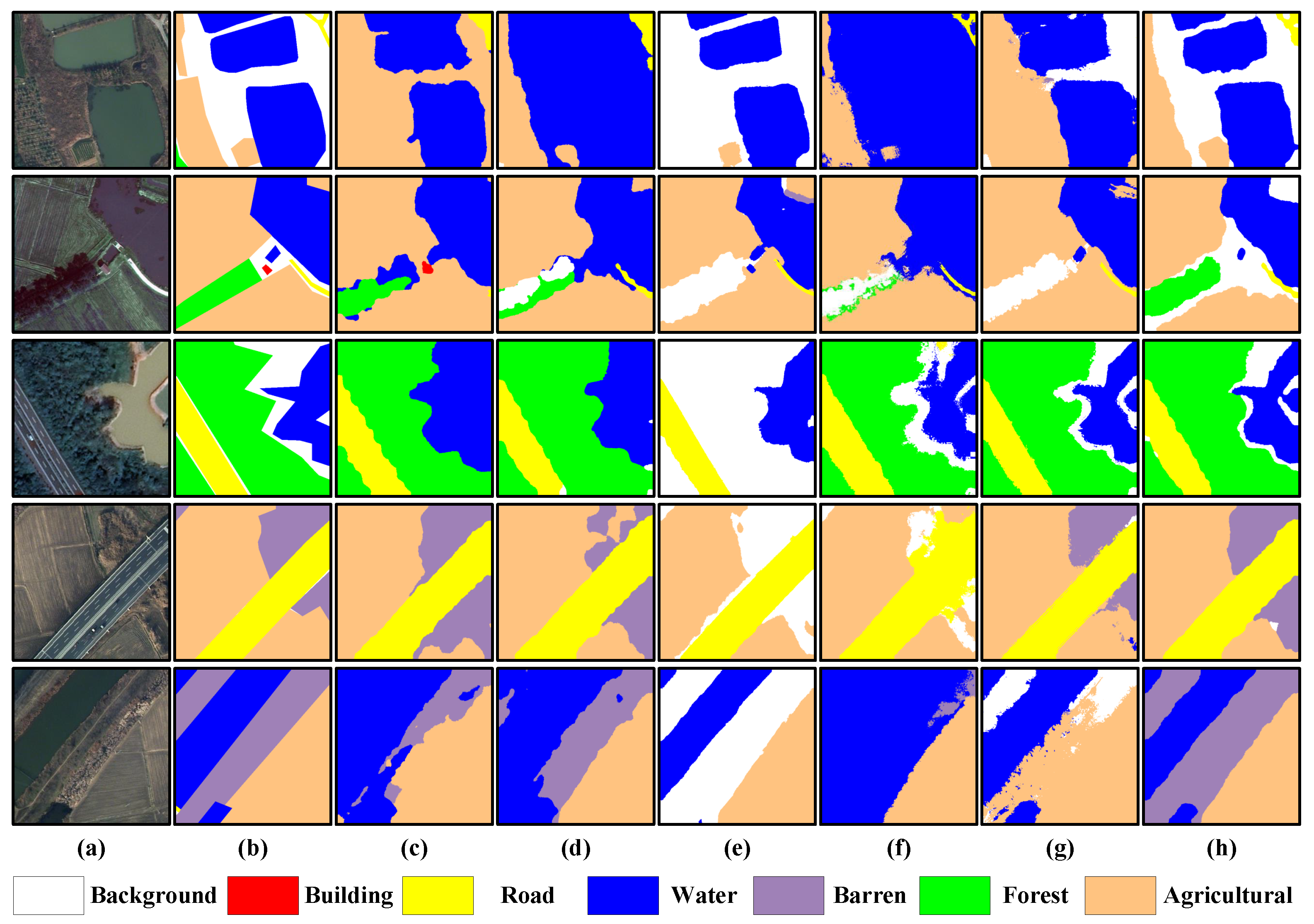
Both quantitative and qualitative comparisons are conducted on the LoveDA dataset, with the qualitative results illustrated in Figure 5 and the quantitative results summarized in

Table 2. Per-class and overall comparison with state-of-the-art WSSS methods on the LoveDA dataset, together with their runtime. Bold values indicate the best result in each column. For runtime, lower is better.

Method	Background	Building	Road	Water	Barren	Forest	Agriculture	mIoU (%)	Time (min)
CTFA [6]	40.14	38.41	43.79	44.02	37.05	50.23	63.48	45.30	238
MoRe [26]	14.33	37.82	46.82	48.73	34.06	50.57	63.65	42.28	236
WeCLIP+ [30]	39.27	44.12	51.29	64.31	13.85	40.51	57.17	44.36	491
PCRE [27]	40.89	18.14	35.72	61.44	21.46	57.77	74.21	44.23	637
ATSG [37]	45.21	43.37	47.71	69.14	39.27	53.49	62.28	51.50	751
Ours	50.34	44.54	50.65	59.59	40.04	58.38	65.04	52.66	454

. As shown in Table 2, the proposed method achieves an mIoU improvement of 1.16 percentage points over the second-best method ATSG and 7.36 percentage points over CTFA. Among the seven semantic categories, the proposed method achieves the best performance on Background, Building, Barren, and Forest, and ranks second on Road and Agriculture. Overall, the proposed method exhibits a well-balanced advantage on LoveDA: rather than relying on extreme high scores in a few categories to inflate the overall mIoU, it consistently ranks at the top across the majority of classes. This characteristic is well aligned with the practical conditions of remote sensing imagery, where land-cover categories densely coexist and mutually suppress each other’s responses.

To further evaluate computational efficiency, we report the runtime of all methods in the last column of Table 2. As shown in Table 2, the proposed framework requires 454 min, which is lower than the 491 min required by WeCLIP+, the 637 min required by PCRE, and the 751 min required by ATSG. Its runtime is higher than the 238 min required by CTFA and the 236 min required by MoRe. Although the proposed framework does not achieve the shortest runtime, it obtains the highest mIoU of 52.66%. These results indicate that the proposed method achieves a favorable trade-off between computational efficiency and segmentation performance on the LoveDA dataset.

Figure 5 presents the qualitative visualization of the proposed method and the competing baselines on the LoveDA dataset. In the first and fourth rows, ATSG and WeCLIP+ exhibit substantial inter-class confusion between Background and Agriculture, misclassifying portions of Background regions as Agriculture; in contrast, by exploiting the CLIP supervision signal fine-tuned with the lightweight adapter and the multi-label decoupled distillation mechanism, the proposed method outperforms the baselines in both boundary completeness and class discriminability. In the second row, although MoRe successfully segments a very small Building, it produces inter-class confusion between Forest and Water, misclassifying Forest as Water, which reflects the limitations of methods lacking CLIP-based prior constraints in cross-class semantic alignment. In the third row, although the segmentation results of ATSG and PCRE are similar in overall shape to those of the proposed method, both exhibit pronounced jagged boundaries; in contrast, with semantic-guided pseudo-label refinement, the proposed method produces smoother boundaries and more consistent class attribution that more faithfully follow the true land-cover contours. In the fifth row, WeCLIP+ fails to correctly segment either the Water class or the Barren class, whereas the proposed method precisely activates small-scale targets through the core-point prompts and tight bounding-box prompts of the SSC module, achieving more accurate segmentation of the small dark-blue water body.

4.3.3. Results on the DeepGlobe Dataset

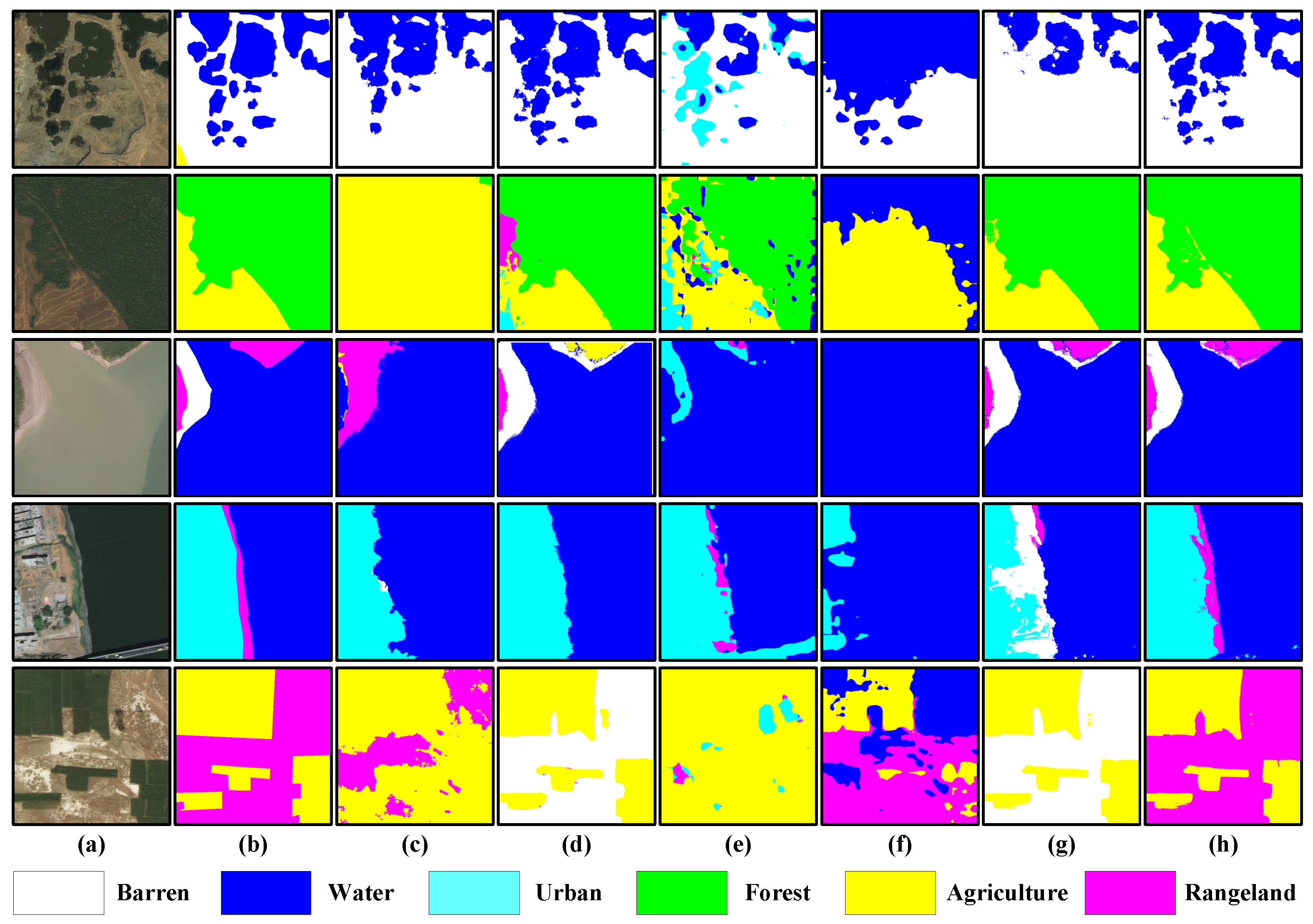
Both quantitative and qualitative comparisons are conducted on the DeepGlobe dataset, with the qualitative results illustrated in Figure 6 and the quantitative results summarized in

Table 3. Per-class and overall comparison with state-of-the-art WSSS methods on the DeepGlobe dataset, together with their runtime. Bold values indicate the best result in each column. For runtime, lower is better.

Method	Urban	Agriculture	Rangeland	Forest	Water	Barren	mIoU (%)	Time (min)
CTFA [6]	63.93	83.21	23.63	78.95	68.36	52.19	61.71	255
MoRe [26]	63.67	78.83	14.80	61.05	64.72	53.45	56.09	264
WeCLIP+ [30]	54.77	78.67	18.00	70.18	72.06	35.73	54.90	255
PCRE [27]	79.86	85.49	2.59	73.48	38.59	58.26	56.38	348
ATSG [37]	69.18	80.98	21.22	75.49	71.80	49.74	61.40	1066
Ours	63.10	81.39	31.71	77.89	72.67	51.12	62.98	429

. As shown in Table 3, the proposed method achieves mIoU improvements of 1.27 percentage points over CTFA and 1.58 percentage points over ATSG. Among the six semantic categories, the proposed method achieves the best performance on Rangeland and Water, and maintains high performance on Forest and Agriculture. It is particularly noteworthy that Rangeland is widely recognized as a difficult class in DeepGlobe due to its small area, scattered distribution, texture similarity to farmland and barren land, and relatively rare samples in the dataset; consequently, most competing methods perform poorly on this class, with PCRE reaching only 2.59% and MoRe only 14.80%. In contrast, the proposed method achieves 31.71% on this class, outperforming CTFA by 8.08 percentage points and ATSG by 10.49 percentage points. This substantial advantage is attributable to the SSC module, which constructs core-point prompts guided by probability maps and tight bounding-box prompts, providing precise geometric constraints for SAM on small-scale, low-response categories and thereby preventing the generation of large irrelevant masks induced by prompt failure.

To further evaluate computational efficiency, we report the runtime of all methods in the last column of Table 3. As shown in Table 3, the proposed framework requires 429 min, which is substantially lower than the 1066 min required by ATSG. However, its runtime is higher than the 255 min required by CTFA and WeCLIP+, the 264 min required by MoRe, and the 348 min required by PCRE. Although the proposed framework does not achieve the shortest runtime, it obtains the highest mIoU of 62.98%. These results provide a quantitative assessment of the computational overhead introduced by the proposed framework and demonstrate the trade-off between runtime and segmentation performance on the DeepGlobe dataset.

Figure 6 presents the qualitative visualization of the proposed method and the competing baselines on the DeepGlobe dataset. In the first row, both WeCLIP+ and PCRE produce noticeable inter-class misclassifications: WeCLIP+ misclassifies portions of the Water region as Urban, while PCRE misclassifies portions of the Barren region as Water; in contrast, the proposed method effectively avoids such inter-class prompt interference at the boundaries with the help of the tight bounding-box and core-point prompts of the SSC module. In the second and fifth rows, the proposed method outperforms the baselines in terms of boundary completeness, an advantage directly attributable to the high-quality boundary delineation produced by SAM under precise prompts in Stage 2 and the further boundary convergence achieved by retraining with refined pseudo-labels in Stage 3. In the third row, the input image contains two texturally and chromatically similar categories, Water and Rangeland, that are easily confused by most competing methods; in contrast, the proposed method successfully distinguishes the two, confirming that the CLIP-based decoupled distillation effectively alleviates the inter-class probability competition among semantically similar categories, enabling each category to be optimized independently. In the fourth row, ATSG misclassifies portions of the Urban region as Barren, while CTFA and MoRe almost entirely fail to identify the Rangeland class; in contrast, through the synergy of CLIP-based semantic priors and SAM-based boundary refinement, the proposed method is able to simultaneously segment categories of high discriminative difficulty.

4.3.4. Boundary Quality Analysis

To quantitatively assess the boundary delineation quality of semantic segmentation results, we further adopt mean Boundary Intersection-over-Union (mBIoU) to evaluate boundary performance on the Potsdam dataset. Potsdam is selected as the representative benchmark because its high spatial resolution, dense urban layout, and numerous small or closely adjacent objects make it particularly challenging for evaluating boundary localization and region separation. For each semantic class, Boundary IoU is calculated between the boundary regions extracted from the prediction and the corresponding ground truth, and the resulting class-wise scores are averaged over the six evaluated categories. The boundary width is defined as

$$d=\max \left(1,\mathrm{round}\left(0.005\sqrt{H^2+W^2}\right)\right),$$

(20)

which corresponds to four pixels for the $512\times 512$ evaluation patches. All methods are evaluated using the same boundary width and evaluation protocol, with ignore-label pixels excluded from the calculation.

As shown in

Table 4. Quantitative boundary-quality comparison on the Potsdam dataset. Bold values indicate the best result.

Method	mBIoU (%)
CTFA [6]	14.12
MoRe [26]	13.79
WeCLIP+ [30]	16.04
PCRE [27]	12.27
ATSG [37]	14.94
Ours	16.49

, the proposed method achieves the highest mBIoU of 16.49%, outperforming the second-best method WeCLIP+ by 0.45 percentage points. The absolute mBIoU values are lower than the corresponding region-level mIoU values because mBIoU evaluates only narrow regions around semantic boundaries and is therefore highly sensitive to small contour displacements. Nevertheless, the results obtained under the unified evaluation protocol demonstrate that the proposed method provides more accurate boundary delineation than the competing methods.

4.3.5. Comparison with Fully Supervised Methods

To further analyze the performance gap between image-level weak supervision and full supervision, we compare our method with the three aforementioned fully supervised models on the LoveDA and DeepGlobe datasets. These models are trained using dense pixel-level annotations, whereas our method uses only image-level annotations. Both the overall mIoU and class-wise IoU are reported to assess the overall performance gap and category-specific differences.

As shown in

Table 5. Comparison between the proposed method and fully supervised methods on the LoveDA dataset. Bold values indicate the best result in each column.

Method	Background	Building	Road	Water	Barren	Forest	Agriculture	mIoU (%)
UNetFormer [49]	57.57	50.51	56.52	70.79	41.92	61.80	68.33	58.21
PIDNet [50]	56.38	51.12	54.58	70.76	37.66	60.94	66.69	56.87
DeepKANSeg [51]	57.14	54.33	53.24	70.93	39.62	62.69	67.08	57.85
Ours	50.34	44.54	50.65	59.59	40.04	58.38	65.04	52.66

and

Table 6. Comparison between the proposed method and fully supervised methods on the DeepGlobe dataset. Bold values indicate the best result in each column.

Method	Urban	Agriculture	Rangeland	Forest	Water	Barren	mIoU (%)
UNetFormer [49]	75.49	86.07	40.00	81.32	75.08	67.75	70.95
PIDNet [50]	75.91	86.33	38.22	82.02	76.50	66.43	70.90
DeepKANSeg [51]	74.98	87.31	40.51	79.79	77.92	70.37	71.81
Ours	63.10	81.39	31.71	77.89	72.67	51.12	62.98

, the fully supervised methods generally achieve higher segmentation accuracy because they benefit from dense pixel-level annotations during training. On LoveDA, our method achieves an mIoU of 52.66%, which is 5.55 percentage points lower than the best fully supervised result of 58.21% obtained by UNetFormer. Nevertheless, our method shows relatively competitive performance on the Barren, Forest, and Agriculture classes. In particular, it achieves an IoU of 40.04% for Barren, outperforming PIDNet and remaining only 1.88 percentage points below the best fully supervised result. On DeepGlobe, our method obtains an mIoU of 62.98%, corresponding to a gap of 8.83 percentage points from the best fully supervised result of 71.81% achieved by DeepKANSeg. Relatively smaller performance gaps are observed for Agriculture, Forest, and Water, whereas larger differences remain for Urban, Rangeland, and Barren. The larger differences for these categories may be attributed to their considerable intra-class variations and inter-class visual similarities, which make it difficult to generate complete and accurate semantic regions using only image-level annotations. Overall, these results quantitatively reveal the remaining performance gap between image-level weak supervision and full supervision while demonstrating that the proposed method achieves reasonable class-wise and overall segmentation performance without requiring dense pixel-level annotations.

4.3.6. Model Complexity and Inference Efficiency

To complement the accuracy comparisons, we evaluate the model complexity and inference efficiency of all methods on the Potsdam, LoveDA, and DeepGlobe datasets. All methods are profiled on an NVIDIA GeForce RTX 4090 using FP32 inference with a batch size of 1 and an input resolution of $512\times 512$. FPS is averaged over 200 forward passes after 50 warm-up iterations. The corresponding Params and FPS results are summarized in

Table 7. Comparison of model complexity and inference speed on the Potsdam, LoveDA, and DeepGlobe datasets. Bold values indicate the best result in each column.

Method	Potsdam		LoveDA		DeepGlobe
	Params (M) ↓	FPS ↑	Params (M) ↓	FPS ↑	Params (M) ↓	FPS ↑
CTFA [6]	111.46	92.49	111.50	94.49	111.49	94.50
MoRe [26]	94.68	80.74	94.71	80.94	94.68	80.61
WeCLIP+ [30]	174.61	65.88	174.61	63.53	174.61	63.52
PCRE [27]	165.08	50.55	165.14	50.78	165.11	51.06
ATSG [37]	111.50	73.76	111.50	73.58	111.49	73.56
Ours	112.49	72.96	115.97	94.41	111.50	94.33

.

As shown in Table 7, MoRe has the smallest parameter count, whereas CTFA achieves the highest FPS on all three datasets. Our method requires substantially fewer parameters than WeCLIP+ and PCRE and has a model size comparable to CTFA and ATSG. On LoveDA and DeepGlobe, our method achieves 94.41 and 94.33 FPS, respectively, closely approaching the corresponding CTFA results of 94.49 and 94.50 FPS. On Potsdam, our method reaches 72.96 FPS, remaining faster than WeCLIP+ and PCRE and comparable to ATSG. Together with the accuracy improvements reported in the preceding comparisons, these results demonstrate that the proposed method achieves a favorable balance between segmentation accuracy, model complexity, and inference efficiency.

4.4. Ablation Study

To systematically evaluate the contribution of each core component in the proposed framework, extensive ablation experiments are conducted on the LoveDA dataset. The evaluation primarily relies on five segmentation performance metrics, namely mean Intersection-over-Union (mIoU), overall accuracy (OA), F1 score, Precision, and Recall, to comprehensively characterize the impact of each component. In addition, for the ablation study on the scale of vision foundation models, two computational cost metrics, parameter count (Params) and frames per second (FPS), are further introduced to balance segmentation accuracy and inference efficiency.

4.4.1. Lightweight Fine-Tuning and Multi-Label Decoupled Distillation Based on CLIP

A component-wise ablation is conducted on the three key components in Stage 1, namely Frozen CLIP backbone, residual adapter (R-Adapter), and decoupled distillation (D-Distill), with the quantitative results summarized in

Table 8. Ablation study on the CLIP-based lightweight fine-tuning and multi-label decoupled distillation. Bold values indicate the best result in each column.

Frozen CLIP	R-Adapter	D-Distill	mIoU	OA	F1	Precision	Recall
			45.30	63.71	61.92	59.88	66.78
✓			48.35	66.34	64.74	63.05	68.24
✓		✓	48.40	67.36	64.72	65.00	65.99
✓	✓		49.45	67.10	65.72	63.85	69.58
✓	✓	✓	50.22	68.49	66.44	66.42	67.89

.

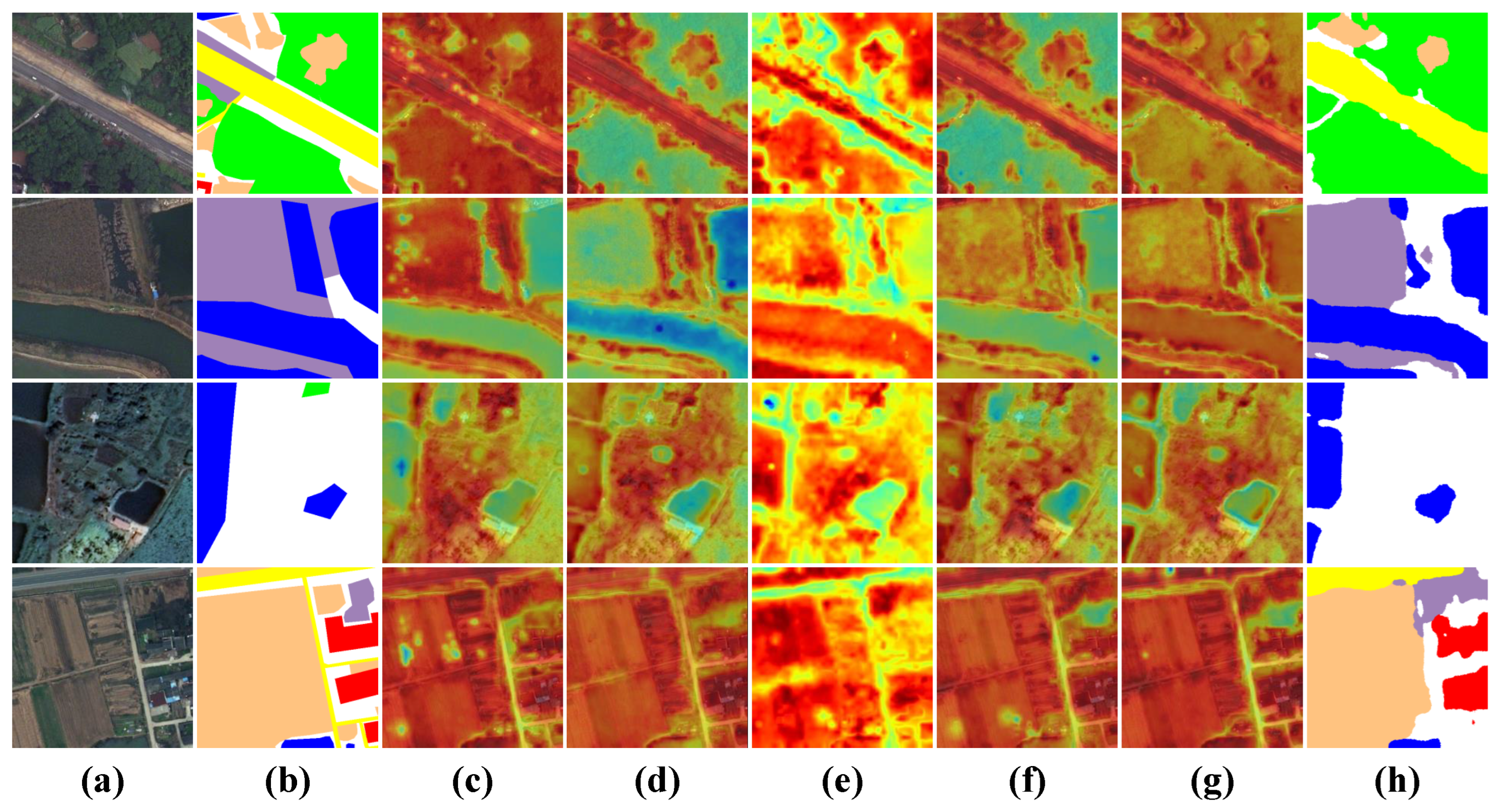
Under the baseline configuration where no CLIP-related component is introduced, the model achieves only 45.30% mIoU and 61.92% F1, reflecting the inherent limitations of a pure ViT backbone under weakly supervised settings. Introducing the frozen CLIP backbone as an additional vision–language prior boosts mIoU by 3.05% and F1 by 2.82%, demonstrating the direct benefit of CLIP’s cross-modal semantic representation for the completeness of initial CAMs. Further introducing the D-Distill mechanism yields a substantial gain of 1.95% in Precision but only a marginal mIoU improvement of 0.05%, suggesting that the distillation mechanism alone can optimize the classification response distribution, but its contribution to final segmentation accuracy remains limited without dedicated feature adaptation to the remote sensing domain. When the R-Adapter is introduced for lightweight adaptation, mIoU is further improved by 1.10%, with Recall reaching 69.58%, validating the effectiveness of the adapter in domain transfer. Finally, the full configuration combining R-Adapter and D-Distill achieves the best results, with mIoU, OA, and F1 improving by 4.92%, 4.78%, and 4.52% over the baseline, respectively. Notably, introducing D-Distill results in a consistent precision–recall trade-off under both configurations. Without R-Adapter, D-Distill increases Precision from 63.05% to 65.00%, while Recall decreases from 68.24% to 65.99%. When combined with R-Adapter, D-Distill further increases Precision from 63.85% to 66.42%, while Recall decreases from 69.58% to 67.89%. This occurs because D-Distill calibrates the category responses toward the CLIP-derived soft targets, reducing ambiguous and cross-class false-positive activations, but it may also suppress some weakly activated true-positive regions. Nevertheless, in the full configuration, the improvements of 0.77, 1.39, and 0.72 percentage points in mIoU, OA, and F1, respectively, demonstrate that the reduction in false-positive predictions outweighs the moderate decrease in Recall, resulting in better overall segmentation performance. These results confirm the functional complementarity between R-Adapter and D-Distill: the former addresses the question of how features should be adapted to the remote sensing domain, while the latter handles how class responses should be independently optimized—together forming the indispensable foundation for high-quality initial CAM generation. The corresponding qualitative CAM comparison is shown in Figure 7. It can be observed that the baseline CAM exhibits pronounced internal holes and severe cross-class adhesion on large homogeneous land covers: introducing Frozen CLIP improves the overall completeness of the activation regions; when only D-Distill is added, the inter-class response distribution begins to decouple, but the fit to land-cover contours remains coarse due to the lack of domain adaptation; further introducing R-Adapter brings the activation regions closer to the true land-cover morphology; and the final full configuration produces high-quality CAMs with sharp boundaries and complete internal activations.

4.4.2. Effectiveness of the DSD and SSC Modules

This subsection validates the contributions of the two core modules in Stage 2, DSD and SSC, to pseudo-label refinement, with the quantitative results summarized in

Table 9. Ablation study on the DSD and SSC modules. Bold values indicate the best result in each column.

DSD	SSC	mIoU	OA	F1	Precision	Recall
		49.51	66.39	65.92	65.97	67.17
✓		50.38	67.40	66.68	68.35	66.67
	✓	50.75	67.19	67.04	68.05	67.87
✓	✓	51.13	67.62	67.37	68.19	68.45

.

Notably, the baseline in this stage represents the model that inherits the Stage 1 weights but applies no DSD or SSC refinement, yielding an mIoU of only 49.51%. As shown in Table 9, introducing the DSD module alone improves mIoU by 0.87% and Precision by 2.38%. This gain primarily originates from the semantic decomposition of large homogeneous connected regions enabled by the high-dimensional semantic consistency of DINOv2, demonstrating that DSD effectively suppresses SAM’s cross-class misactivation in adhered regions. Introducing the SSC module alone yields improvements of 1.24% in mIoU, 2.08% in Precision, and 0.70% in Recall, reflecting the contribution of probability-guided core-point prompts and tight bounding-box prompts to the complete coverage of land covers. When DSD and SSC are jointly applied, the joint configuration achieves the best mIoU, OA, F1, and Recall, while maintaining Precision close to that of the DSD-only configuration, with mIoU, OA, F1, Precision, and Recall improving by 1.62%, 1.23%, 1.45%, 2.22%, and 1.28% over the baseline, respectively. These results reveal the complementary roles of the two modules along different dimensions: DSD focuses on “semantic decoupling” to enhance Precision, while SSC focuses on “prompt refinement” to safeguard Recall, jointly achieving simultaneous optimization of Precision and Recall.

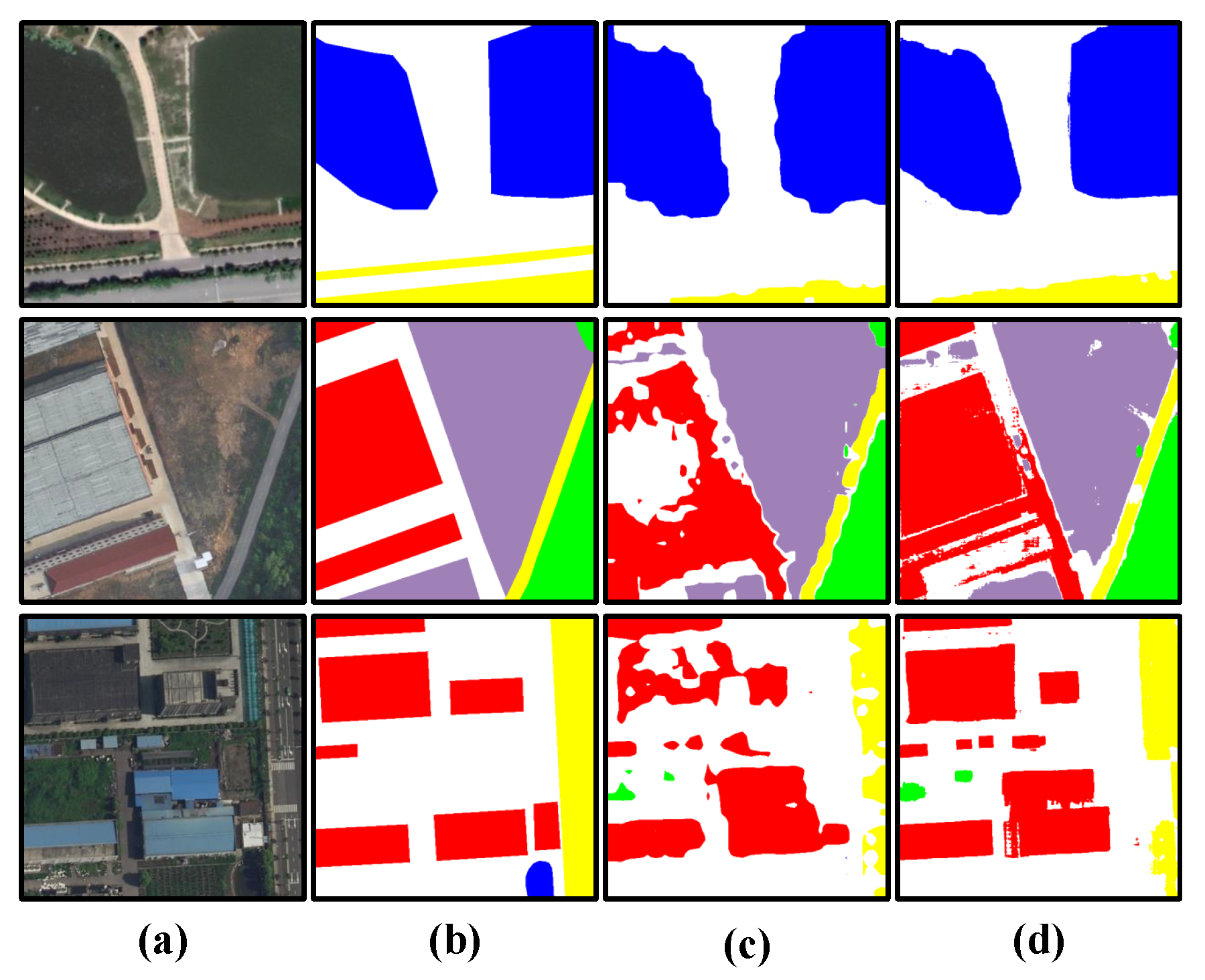
To more intuitively illustrate the synergistic refinement effect of DSD and SSC, Figure 8 further provides a qualitative comparison between RSM and RPL. In the forward pipeline of Stage 2, multi-branch probability fusion and confidence filtering first generate the Reliable Seed Mask (RSM), which is then jointly refined by the DINOv2-guided semantic decomposition and the Spatial–Semantic Constraint modules to produce the Refined Pseudo-Labels (RPL) with reliable class attribution, providing high-quality pixel-level supervision for the end-to-end segmentation network in Stage 3. As shown in Figure 8, the RSM exhibits pronounced internal holes and boundary adhesion on the red category in the second and third rows, whereas the RPL refined by DSD and SSC shows substantial improvements in internal completeness, boundary sharpness, and class attribution consistency.

4.4.3. Ablation Study on the Confidence Threshold $\tau$

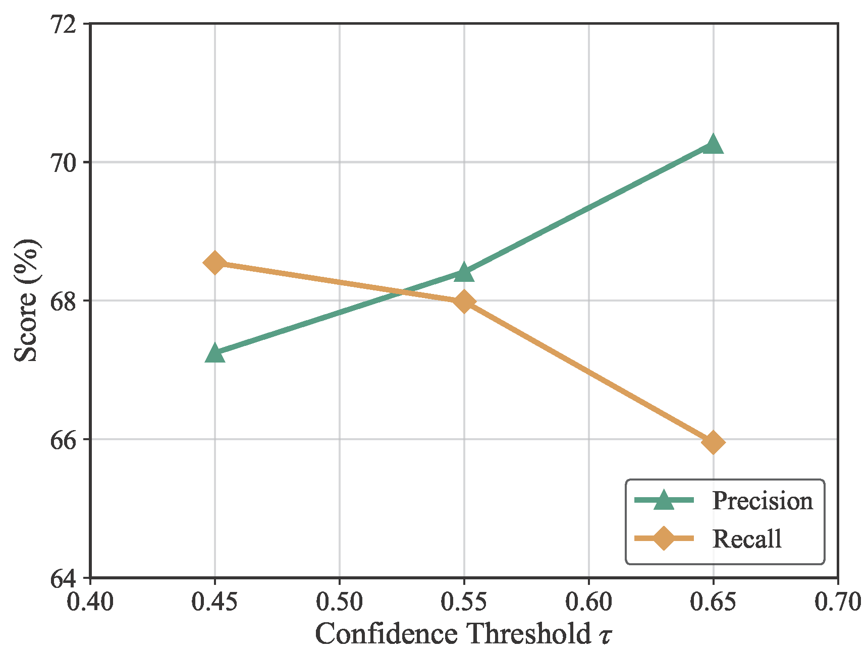
The confidence threshold $\tau$ controls the trade-off between reliable pixels and ignored pixels in the RSM: an excessively low threshold retains too much noise, while an excessively high threshold discards a large number of valid seeds. In this subsection, three candidate values of $\tau \in \{0.45, 0.55, 0.65\}$ are systematically evaluated, with the quantitative results summarized in

Table 10. Ablation study on the confidence threshold $\tau$. Bold values indicate the best result in each column.

$\mathit{\tau }$	mIoU	OA	F1
0.45	50.57	67.11	66.90
0.55	51.13	67.62	67.37
0.65	50.72	67.48	66.98

and the Precision–Recall curves illustrated in Figure 9.

When $\tau =0.45$, the model retains more pixels as reliable seeds, yielding the highest Recall; however, the inclusion of low-confidence pixels also introduces additional noise, leading to relatively low Precision. When $\tau =0.55$, the model achieves the optimal balance between Precision and Recall, with mIoU and F1 increasing by 0.56% and 0.47% over the $\tau =0.45$ configuration. When $\tau =0.65$, the strict filtering policy pushes Precision to its highest level, but Recall drops noticeably, indicating that an overly high threshold incorrectly excludes a substantial number of valid pixels, ultimately reducing mIoU by 0.41% relative to the $\tau =0.55$ configuration. These results collectively confirm that $\tau =0.55$ is the most appropriate choice for balancing label purity and coverage completeness.

4.4.4. Ablation Study on the Area Constraint Threshold

In the SSC module, the area constraint threshold $\gamma$ plays a vital role in mitigating excessive background diffusion introduced by SAM during pseudo-label refinement. To systematically investigate the influence of this hyperparameter on segmentation performance, we perform an ablation study using three candidate values: $\gamma \in \{3.0, 4.0, 5.0\}$. The quantitative results are presented in

Table 11. Ablation study on the area constraint threshold $\gamma$. Bold values indicate the best result in each column.

$\mathit{\gamma }$	mIoU (%)	OA (%)	F1 (%)
3.0	50.95	67.45	67.22
4.0	51.13	67.62	67.37
5.0	51.09	67.58	67.33

.

As shown in Table 11, the framework is relatively stable within a moderate range of $\gamma$, with $\gamma =4.0$ achieving the best trade-off. When $\gamma =3.0$, the mIoU reaches only 50.95%, indicating an overly strict area constraint. This severely restricts SAM’s zero-shot boundary expansion and results in under-segmentation. In contrast, setting $\gamma =5.0$ yields an overly loose constraint. The mIoU drops by 0.04% compared with the case of $\gamma =4.0$. This performance degradation mainly occurs because SAM mistakenly merges surrounding background pixels and adjacent regions into the predicted categories, introducing background leakage and causing over-segmentation. The best performance on all three metrics is obtained when $\gamma =4.0$, with mIoU, OA, and F1 reaching 51.13%, 67.62%, and 67.37%, respectively. This threshold achieves an optimal balance between accurate recovery of target boundary features and effective suppression of background noise. Therefore, we adopt $\gamma =4.0$ as the optimal area constraint threshold for the SSC module.

4.4.5. Ablation Study on Vision Foundation Models

To investigate the impact of vision foundation model scale on the overall framework performance, the CLIP encoder and SAM backbone are systematically compared under different model scales, with evaluation metrics covering both segmentation accuracy (mIoU, F1) and computational cost (Params, FPS).

Effect of CLIP encoder scale. As shown in

Table 12. Ablation study on CLIP encoder scale. Bold values indicate the best result in each column.

CLIP	mIoU	F1	Params (M)	FPS
ViT-B/32	48.60	64.89	263.30	53.60
ViT-B/16	47.62	63.92	261.65	53.43
ViT-L/14	50.22	66.44	540.30	47.30

, among the three CLIP encoder variants, ViT-L/14 achieves the best performance, with an mIoU of 50.22% and F1 of 66.44%, outperforming ViT-B/32 and ViT-B/16 by 1.62% and 2.60% in mIoU, and by 1.55% and 2.52% in F1, respectively. Although ViT-L/14 doubles the parameter count of the ViT-B series and reduces the inference speed from 53.60 FPS to 47.30 FPS, the high-quality initial semantic prior it provides during the cold-start phase of weak supervision is crucial for the final performance. Consequently, ViT-L/14 is selected as the CLIP teacher model in this work.

Effect of SAM backbone scale. As shown in

Table 13. Ablation study on SAM backbone scale. Bold values indicate the best result in each column.

SAM	mIoU	F1	Params (M)	FPS
ViT-B	50.15	66.48	93.74	3.44
ViT-H	51.13	67.37	640.09	2.43

, in the SAM backbone comparison, ViT-H outperforms ViT-B across all performance indicators, with mIoU and F1 improving by 0.98% and 0.89%, respectively. This performance gain comes at the cost of an increase in parameters from 93.74M to 640.09M and a decrease in inference speed from 3.44 FPS to 2.43 FPS. However, within the overall paradigm of weakly supervised semantic segmentation, SAM operates only during the offline pseudo-label generation stage, where real-time performance is not critical. It is therefore reasonable to sacrifice a certain amount of offline inference speed in exchange for higher-quality pseudo-labels. Consequently, ViT-H is selected as the SAM backbone in this work.

4.4.6. Ablation Study on the Overall Framework

To validate the cumulative contribution of each core innovation module in the three-stage framework, a progressive ablation is conducted module by module, with the quantitative results summarized in

Table 14. Ablation study on the overall three-stage framework. Adapter-CLIP denotes the CLIP-based decoupled cross-modal distillation module; Semantic-Guided denotes the pseudo-label refinement module comprising DSD and SSC. Bold values indicate the best result in each column.

Baseline	Adapter-CLIP	Semantic-Guided	Retrain	mIoU	OA	F1	Precision	Recall
✓				45.30	63.71	61.92	59.88	66.78
✓	✓			50.22	68.49	66.44	66.42	67.89
✓	✓	✓		51.13	67.62	67.37	68.19	68.45
✓	✓	✓	✓	52.66	70.15	68.61	68.38	69.72

.

The baseline model relies solely on the ViT backbone with image-level labels, achieving only 45.30% mIoU under the impoverished weak supervision setting. After introducing the Adapter-CLIP module, the model leverages the vision–language prior of CLIP to effectively alleviate the localization ambiguity in the early stage of weak supervision, yielding the first substantial performance jump: mIoU, OA, and F1 improve by 4.92%, 4.78%, and 4.52%, respectively. This substantial improvement confirms the critical role of cross-modal semantic priors in the weakly supervised remote sensing task.

Subsequently, the Semantic-Guided strategy (containing both the DSD and SSC modules) is integrated on top of the CAMs produced by Adapter-CLIP to further refine the boundaries of the coarse pseudo-labels. At this stage, mIoU, F1, and Precision are further improved by 0.91%, 0.93%, and 1.77%, respectively. The substantial gain in Precision is particularly noteworthy, as it directly verifies that under precise spatial prompts, SAM successfully eliminates a large amount of background noise and sharpens the dilated semantic activations into high-quality masks tightly aligned with the physical boundaries of land covers. Although OA exhibits a slight drop from 68.49% to 67.62%, this decrease is attributable to the ignore strategy applied to low-confidence pixels during the pseudo-label refinement process, which introduces positions that are not counted as effective predictions at the pixel-total level. This phenomenon is subsequently corrected in the retraining stage.

Finally, the refined pseudo-labels are used as strong supervision signals to retrain the final segmentation network. This stage decouples the model from any reliance on large foundation models during inference and further improves generalization of the segmentation network on remote sensing scenes, leading to convergence across all metrics: mIoU reaches its peak value of 52.66%, a 7.36% improvement over the baseline, while OA, F1, Precision, and Recall improve by 6.44%, 6.69%, 8.50%, and 2.94% over the baseline, respectively. These results not only validate the inherent rationality of the three-stage framework but also confirm the stability and robustness of the progressive learning design.

4.4.7. Computational Efficiency Analysis

To further quantify the computational overhead introduced by the use of multiple foundation models, we present a stage-wise runtime analysis of the proposed framework in

Table 15. Stage-wise runtime analysis of the proposed framework on the three datasets.

Stage	Runtime (min)
	Potsdam	LoveDA	DeepGlobe
CLIP-Based Decoupled Cross-Modal Distillation (Stage 1)	229	256	211
Semantic-Guided Pseudo-Label Refinement (Stage 2)	21	86	122
Warm-Start Retraining (Stage 3)	51	112	96
Total	301	454	429

. The complete framework requires 301, 454, and 429 min on the Potsdam, LoveDA, and DeepGlobe datasets, respectively. As shown in Table 1, Table 2 and Table 3, although the proposed method does not achieve the shortest runtime in all cases, it requires less runtime than PCRE and ATSG on Potsdam, less runtime than WeCLIP+, PCRE, and ATSG on LoveDA, and substantially less runtime than ATSG on DeepGlobe, while achieving the highest mIoU on all three datasets. These results demonstrate that the proposed method achieves a favorable trade-off between computational efficiency and segmentation performance. Specifically, the DINOv2- and SAM-based pseudo-label refinement in Stage 2 accounts for approximately 6.98%, 18.94%, and 28.44% of the complete runtime on Potsdam, LoveDA, and DeepGlobe, respectively. This stage is performed only once as an offline feed-forward process, and the resulting pseudo-labels are subsequently used for warm-start retraining. Moreover, the final segmentation network operates independently of CLIP, DINOv2, and SAM during inference. Therefore, the computational overhead introduced by the foundation models is confined to the offline model-construction process and does not increase the inference-time cost of the deployed segmentation model.

4.4.8. Analysis of CLIP-Related Loss Weights

To analyze the effects of the two CLIP-related loss weights, we conduct one-factor-at-a-time experiments on the LoveDA dataset. When varying ${\lambda }_{\mathrm{clip}}$, ${\lambda }_{\mathrm{distill}}$ is fixed at 0.5; when varying ${\lambda }_{\mathrm{distill}}$, ${\lambda }_{\mathrm{clip}}$ is fixed at 0.2. All other training settings remain unchanged.

As shown in

Table 16. Performance comparison under different CLIP-related loss weights on the LoveDA dataset. Bold values indicate the best-performing setting within each coefficient group.

Coefficient	Value	F1 (%)	OA (%)	mIoU (%)
${\lambda }_{\mathrm{clip}}$	0.1	63.93	66.63	47.81
	0.2	66.44	68.49	50.22
	0.3	65.79	67.79	49.58
${\lambda }_{\mathrm{distill}}$	0.25	65.27	67.56	48.97
	0.50	66.44	68.49	50.22
	1.00	63.41	66.15	47.23

, the model achieves the best performance when ${\lambda }_{\mathrm{clip}}=0.2$, with an F1 score of 66.44%, an OA of 68.49%, and an mIoU of 50.22%. Compared with ${\lambda }_{\mathrm{clip}}=0.1$ and 0.3, this setting improves the mIoU by 2.41 and 0.64 percentage points, respectively. This indicates that weak CLIP supervision may be insufficient for effective domain adaptation, whereas an excessively large coefficient may overemphasize the CLIP adaptation objective. Similarly, ${\lambda }_{\mathrm{distill}}=0.5$ achieves the best results across all three metrics, outperforming 0.25 and 1.0 by 1.25 and 2.99 percentage points in mIoU, respectively. A small coefficient may limit semantic knowledge transfer from the adapted CLIP teacher, while an overly large value may cause teacher supervision to dominate the underlying WSSS objectives. The consistent trends in F1, OA, and mIoU show that ${\lambda }_{\mathrm{clip}}=0.2$ and ${\lambda }_{\mathrm{distill}}=0.5$ provide an appropriate balance between domain adaptation, cross-modal distillation, and WSSS optimization. Therefore, these values are adopted in all subsequent experiments.

4.4.9. Analysis of Multi-Branch Fusion Weights

To evaluate the influence of the fusion coefficients in Equation (5), we conducted an ablation study using six representative weight configurations on the LoveDA dataset. The evaluated configurations range from CAM-only fusion to segmentation-only prediction, thereby progressively increasing the contribution of the segmentation branch. The primary and auxiliary CAMs are assigned equal weights in each configuration because they serve the same auxiliary localization role. Since confidence filtering is applied immediately after probability fusion, the confidence threshold was fixed at $\tau =0.55$ for all configurations to isolate the influence of the fusion coefficients. All other experimental settings remained unchanged. The results are reported in

Table 17. Performance comparison of different multi-branch probability fusion weights on the LoveDA dataset. Bold values indicate the best result for each evaluation metric.

${\mathit{w}}_{\mathit{a}}$ (Seg)	${\mathit{w}}_{\mathit{b}}$ (Aux-CAM)	${\mathit{w}}_{\mathit{c}}$ (CAM)	F1 (%)	OA (%)	mIoU (%)
0.00	0.50	0.50	64.18	63.27	47.76
1/3	1/3	1/3	65.33	67.17	49.10
0.50	0.25	0.25	65.37	67.42	50.09
0.70	0.15	0.15	66.44	68.49	50.22
0.80	0.10	0.10	66.48	67.44	50.13
1.00	0.00	0.00	66.31	67.36	50.01

.

As shown in Table 17, the CAM-only fusion configuration $(w_a,w_b,w_c)$ = $(0.00, 0.50, 0.50)$ produces the lowest performance, with an F1 score of 64.18%, an OA of 63.27%, and an mIoU of 47.76%. In this configuration, the segmentation branch is excluded, while equal weights are assigned to the primary and auxiliary CAM branches. The results indicate that the classification-derived CAMs alone cannot provide sufficiently complete and accurate pixel-level localization. Increasing the contribution of the segmentation branch generally improves the segmentation performance, confirming that its dense pixel-level predictions should play a dominant role in the fusion process.

The configuration $(w_a,w_b,w_c)=(0.70, 0.15, 0.15)$ achieves the highest OA of 68.49% and the highest mIoU of 50.22%. Compared with the equal-weight configuration, it improves F1, OA, and mIoU by 1.11, 1.32, and 1.12 percentage points, respectively. Although $(w_a,w_b,w_c)=(0.80, 0.10, 0.10)$ achieves an F1 score of 66.48%, which is marginally higher than that of the selected configuration by 0.04 percentage points, its OA and mIoU are lower by 1.05 and 0.09 percentage points, respectively.

Moreover, relying exclusively on the segmentation branch results in an mIoU of 50.01%, which is 0.21 percentage points lower than that of the selected configuration. This result demonstrates that the primary and auxiliary CAM branches still provide useful complementary semantic localization cues. Therefore, considering the overall performance, particularly OA and mIoU, $(w_a,w_b,w_c)=(0.70, 0.15, 0.15)$ is selected as the final fusion configuration.

4.4.10. Analysis of Cluster-Number Selection Strategies

To investigate the influence of the cluster-number selection strategy in the DSD module, we compared three configurations on the LoveDA and DeepGlobe datasets: fixed $K=2$, fixed $K=3$, and a predefined area-aware $K=2/3$ rule. Under the area-aware rule, $K=2$ is used when the area of the class-specific candidate mask satisfies $A_c<5000$, whereas $K=3$ is used when $A_c\ge 5000$. The dataset-specific DSD activation thresholds and all other experimental settings were kept unchanged. The quality of the generated pseudo-labels was evaluated using F1, OA, and mIoU, as reported in

Table 18. Pseudo-label quality comparison of different cluster-number selection strategies on the DeepGlobe and LoveDA datasets. Bold values indicate the best result for each dataset.

Dataset	Cluster Strategy	F1 (%)	OA (%)	mIoU (%)
DeepGlobe	Fixed $K=2$	71.60	76.05	59.89
	Fixed $K=3$	71.67	76.20	59.99
	Area-aware $K=2/3$	72.62	77.09	61.27
LoveDA	Fixed $K=2$	67.37	67.62	51.13
	Fixed $K=3$	66.72	66.83	50.35
	Area-aware $K=2/3$	67.29	67.59	51.04

.

As shown in Table 18, the area-aware strategy achieves the best performance on DeepGlobe, reaching an F1 score of 72.62%, an OA of 77.09%, and an mIoU of 61.27%. Compared with fixed $K=2$, it improves F1, OA, and mIoU by 1.02, 1.04, and 1.38 percentage points, respectively. It also outperforms fixed $K=3$ by 0.95, 0.89, and 1.28 percentage points, respectively. These results indicate that applying finer decomposition only to sufficiently large candidate masks is beneficial for the spatially extensive and internally heterogeneous land-cover regions in DeepGlobe. On LoveDA, fixed $K=2$ achieves the best results, with an F1 score of 67.37%, an OA of 67.62%, and an mIoU of 51.13%. The area-aware strategy produces closely comparable results, with decreases of only 0.08, 0.03, and 0.09 percentage points, respectively. In contrast, fixed $K=3$ causes a more evident performance reduction, suggesting that uniformly increasing the cluster number may over-fragment the comparatively compact and fine-grained candidate regions in LoveDA. Therefore, fixed $K=2$ is retained for LoveDA, whereas the predefined area-aware $K=2/3$ rule is adopted for DeepGlobe. These results experimentally justify the dataset-specific cluster-number configurations.

5. Discussion

Remote sensing WSSS remains challenging because image-level supervision often produces incomplete class responses and causes adjacent land-cover regions with similar appearances to be merged. The proposed framework addresses these issues by coordinating complementary priors from CLIP, DINOv2, and SAM. Sigmoid-based decoupled distillation enables independent modeling of co-occurring categories. DINOv2 features help separate heterogeneous regions within merged candidates, while SSC filters SAM-generated masks whose areas substantially exceed those of their corresponding candidate regions and protects high-confidence pixels assigned to other classes from being overwritten. This complementary design indicates that reliable pseudo-label generation requires both semantic calibration and spatially constrained mask refinement.

Despite the strong performance demonstrated across multiple remote sensing datasets, two limitations remain. First, small and rare categories are underrepresented in the training data and occupy only a small fraction of image pixels, making them more susceptible to missed detections. Second, using CLIP, DINOv2, and SAM during training and offline pseudo-label generation increases the computational cost of model construction. Although warm-start retraining enables the final segmentation network to operate independently of foundation models during inference, the offline computational cost remains non-negligible. Future work will investigate class-balanced loss weighting and semi-supervised learning to improve small-target segmentation, as well as lightweight alternatives based on knowledge distillation and model compression to reduce the cost of pseudo-label generation.

6. Conclusions

This paper presented a three-stage framework for weakly supervised semantic segmentation of remote sensing imagery using only image-level labels. In the first stage, a lightweight CLIP adapter and sigmoid-based multi-label decoupled distillation reduce competition among co-occurring land-cover categories and improve the spatial coverage of CAMs. In the second stage, DINOv2 features decompose large merged regions before SAM prompting, while Spatial–Semantic Constraints guide the construction of point-and-box prompts and the filtering of masks to generate more reliable pseudo-labels. In the final stage, a compact segmentation network is warm-started using the weights learned in the first stage and retrained using the refined pseudo-labels. Consequently, only the compact network is retained during inference, without requiring CLIP, DINOv2, or SAM.

The proposed method achieved mIoU scores of 53.16%, 52.66%, and 62.98% on Potsdam, LoveDA, and DeepGlobe, respectively, outperforming the strongest competing baseline on each dataset by 6.55, 1.16, and 1.27 percentage points, respectively. The ablation studies further demonstrated the complementary contributions of decoupled cross-modal distillation, semantically guided pseudo-label refinement, and warm-start retraining. Nevertheless, the segmentation of small and rare categories remains challenging, and the use of multiple foundation models increases the computational cost of training and offline pseudo-label generation. Future work will focus on improving small and rare category segmentation and developing more efficient pseudo-label refinement strategies.

References

1. Wang, J.; Zheng, Z.; Ma, A.; Lu, X.; Zhong, Y. LoveDA: A Remote Sensing Land-Cover Dataset for Domain Adaptive Semantic Segmentation. In Proceedings of the Neural Information Processing Systems Track on Datasets and Benchmarks; Vanschoren, J., Yeung, S., Eds.; Curran Associates, Inc.: Red Hook, NY, USA, 2021; Volume 1. [Google Scholar]
2. Milioto, A.; Lottes, P.; Stachniss, C. Real-Time Semantic Segmentation of Crop and Weed for Precision Agriculture Robots Leveraging Background Knowledge in CNNs. In Proceedings of the 2018 IEEE International Conference on Robotics and Automation (ICRA), Brisbane, Australia, 21–25 May 2018; pp. 2229–2235. [Google Scholar] [CrossRef] [Scilit]
3. Liu, Y.; Li, Q.; Yuan, Y.; Du, Q.; Wang, Q. ABNet: Adaptive Balanced Network for Multiscale Object Detection in Remote Sensing Imagery. IEEE Trans. Geosci. Remote Sens. 2022, 60, 5614914. [Google Scholar] [CrossRef] [Scilit]
4. Zhang, L.; Zhang, L. Artificial Intelligence for Remote Sensing Data Analysis: A review of challenges and opportunities. IEEE Geosci. Remote Sens. Mag. 2022, 10, 270–294. [Google Scholar] [CrossRef] [Scilit]
5. Dosovitskiy, A.; Beyer, L.; Kolesnikov, A.; Weissenborn, D.; Zhai, X.; Unterthiner, T.; Dehghani, M.; Minderer, M.; Heigold, G.; Gelly, S.; et al. An Image is Worth 16x16 Words: Transformers for Image Recognition at Scale. In Proceedings of the International Conference on Learning Representations, Virtual, 3–7 May 2021. [Google Scholar]
6. Hu, Z.; Gao, J.; Yuan, Y.; Li, X. Contrastive Tokens and Label Activation for Remote Sensing Weakly Supervised Semantic Segmentation. IEEE Trans. Geosci. Remote Sens. 2024, 62, 5620211. [Google Scholar] [CrossRef] [Scilit]
7. Zhou, B.; Khosla, A.; Lapedriza, A.; Oliva, A.; Torralba, A. Learning Deep Features for Discriminative Localization. In Proceedings of the 2016 IEEE Conference on Computer Vision and Pattern Recognition (CVPR), Las Vegas, NV, USA, 27–30 June 2016; pp. 2921–2929. [Google Scholar] [CrossRef] [Scilit]
8. Selvaraju, R.R.; Cogswell, M.; Das, A.; Vedantam, R.; Parikh, D.; Batra, D. Grad-CAM: Visual Explanations from Deep Networks via Gradient-Based Localization. In Proceedings of the 2017 IEEE International Conference on Computer Vision (ICCV), Venice, Italy, 22–29 October 2017; pp. 618–626. [Google Scholar] [CrossRef] [Scilit]
9. Ahn, J.; Kwak, S. Learning Pixel-Level Semantic Affinity with Image-Level Supervision for Weakly Supervised Semantic Segmentation. In Proceedings of the 2018 IEEE/CVF Conference on Computer Vision and Pattern Recognition, Salt Lake City, UT, USA, 18–23 June 2018; pp. 4981–4990. [Google Scholar] [CrossRef] [Scilit]
10. Wang, Y.; Zhang, J.; Kan, M.; Shan, S.; Chen, X. Self-Supervised Equivariant Attention Mechanism for Weakly Supervised Semantic Segmentation. In Proceedings of the 2020 IEEE/CVF Conference on Computer Vision and Pattern Recognition (CVPR), Seattle, WA, USA, 13–19 June 2020; pp. 12272–12281. [Google Scholar] [CrossRef] [Scilit]
11. Zhou, R.; Zhang, W.; Yuan, Z.; Rong, X.; Liu, W.; Fu, K.; Sun, X. Weakly Supervised Semantic Segmentation in Aerial Imagery via Explicit Pixel-Level Constraints. IEEE Trans. Geosci. Remote Sens. 2022, 60, 5634517. [Google Scholar] [CrossRef] [Scilit]
12. Jiang, P.T.; Yang, Y.; Hou, Q.; Wei, Y. L2G: A Simple Local-to-Global Knowledge Transfer Framework for Weakly Supervised Semantic Segmentation. In Proceedings of the 2022 IEEE/CVF Conference on Computer Vision and Pattern Recognition (CVPR), New Orleans, LA, USA, 18–24 June 2022; pp. 16865–16875. [Google Scholar] [CrossRef] [Scilit]
13. Radford, A.; Kim, J.W.; Hallacy, C.; Ramesh, A.; Goh, G.; Agarwal, S.; Sastry, G.; Askell, A.; Mishkin, P.; Clark, J.; et al. Learning Transferable Visual Models From Natural Language Supervision. In Proceedings of the 38th International Conference on Machine Learning, ICML 2021, Virtual Event, 18–24 July 2021; Meila, M., Zhang, T., Eds.; Proceedings of Machine Learning Research (PMLR): Cambridge, MA, USA, 2021; pp. 8748–8763. [Google Scholar]
14. Oquab, M.; Darcet, T.; Moutakanni, T.; Vo, H.V.; Szafraniec, M.; Khalidov, V.; Fernandez, P.; Haziza, D.; Massa, F.; El-Nouby, A.; et al. DINOv2: Learning Robust Visual Features without Supervision. Trans. Mach. Learn. Res. 2024. [Google Scholar] [CrossRef] [Scilit]
15. Kirillov, A.; Mintun, E.; Ravi, N.; Mao, H.; Rolland, C.; Gustafson, L.; Xiao, T.; Whitehead, S.; Berg, A.C.; Lo, W.Y.; et al. Segment Anything. In Proceedings of the IEEE/CVF International Conference on Computer Vision (ICCV), Paris, France, 1–6 October 2023; pp. 4015–4026. [Google Scholar]
16. Zhang, L.; Huang, W.; Fan, B. SARFormer: Segmenting Anything Guided Transformer for semantic segmentation. Neurocomputing 2025, 635, 129915. [Google Scholar] [CrossRef] [Scilit]
17. Cheng, T.; Wang, X.; Chen, S.; Zhang, Q.; Liu, W. BoxTeacher: Exploring High-Quality Pseudo Labels for Weakly Supervised Instance Segmentation. In Proceedings of the 2023 IEEE/CVF Conference on Computer Vision and Pattern Recognition (CVPR), Vancouver, BC, Canada, 17–24 June 2023; pp. 3145–3154. [Google Scholar] [CrossRef] [Scilit]
18. Long, J.; Shelhamer, E.; Darrell, T. Fully convolutional networks for semantic segmentation. In Proceedings of the 2015 IEEE Conference on Computer Vision and Pattern Recognition (CVPR), Boston, MA, USA, 7–12 June 2015; pp. 3431–3440. [Google Scholar] [CrossRef] [Scilit]
19. Ronneberger, O.; Fischer, P.; Brox, T. U-Net: Convolutional Networks for Biomedical Image Segmentation. In Proceedings of the Medical Image Computing and Computer-Assisted Intervention—MICCAI 2015; Navab, N., Hornegger, J., Wells, W.M., Frangi, A.F., Eds.; Springer: Cham, Switzerland, 2015; pp. 234–241. [Google Scholar]
20. Xie, E.; Wang, W.; Yu, Z.; Anandkumar, A.; Alvarez, J.M.; Luo, P. SegFormer: Simple and Efficient Design for Semantic Segmentation with Transformers. In Proceedings of the Advances in Neural Information Processing Systems; Ranzato, M., Beygelzimer, A., Dauphin, Y., Liang, P., Vaughan, J.W., Eds.; Curran Associates, Inc.: Red Hook, NY, USA, 2021; Volume 34, pp. 12077–12090. [Google Scholar]
21. Zhang, Y.; Cheng, J.; Su, Y.; Deng, C.; Xia, Z.; Tashi, N. Global Adaptive Second-Order Transformer for Remote Sensing Image Semantic Segmentation. IEEE Trans. Geosci. Remote Sens. 2024, 62, 5640417. [Google Scholar] [CrossRef] [Scilit]
22. Wu, Y.; Wang, F.; Zhao, P.; Zhou, M.; Geng, S.; Zhang, D. UNet with Multibranch Prior Information Encoding for Building Segmentation in Remote Sensing Images. Adv. Space Res. 2025, 76, 4296–4313. [Google Scholar] [CrossRef] [Scilit]
23. Chen, K.; Zou, Z.; Shi, Z. Building Extraction from Remote Sensing Images with Sparse Token Transformers. Remote Sens. 2021, 13, 4441. [Google Scholar] [CrossRef] [Scilit]
24. Chen, Z.; Sun, Q. Weakly-supervised Semantic Segmentation with Image-level Labels: From Traditional Models to Foundation Models. ACM Comput. Surv. 2024, 57, 111. [Google Scholar] [CrossRef] [Scilit]
25. Caron, M.; Touvron, H.; Misra, I.; Jegou, H.; Mairal, J.; Bojanowski, P.; Joulin, A. Emerging Properties in Self-Supervised Vision Transformers. In Proceedings of the 2021 IEEE/CVF International Conference on Computer Vision (ICCV), Montreal, QC, Canada, 10–17 October 2021; pp. 9630–9640. [Google Scholar] [CrossRef] [Scilit]
26. Yang, Z.; Meng, Y.; Fu, K.; Wang, S.; Song, Z. MoRe: Class patch attention needs regularization for weakly supervised semantic segmentation. In Proceedings of the Thirty-Ninth AAAI Conference on Artificial Intelligence and Thirty-Seventh Conference on Innovative Applications of Artificial Intelligence and Fifteenth Symposium on Educational Advances in Artificial Intelligence (AAAI Press, 2025, AAAI’25/IAAI’25/EAAI’25), Philadelphia, PA, USA, 25 February–4 March 2025. [Google Scholar] [CrossRef] [Scilit]
27. Xu, X.; Zhang, P.; Huang, W.; Shen, Y.; Chen, H.; Lin, J.; Li, W.; He, G.; Xie, J.; Lin, S. Weakly Supervised Semantic Segmentation via Progressive Confidence Region Expansion. In Proceedings of the 2025 IEEE/CVF Conference on Computer Vision and Pattern Recognition (CVPR), Nashville, TN, USA, 10–17 June 2025; pp. 9829–9838. [Google Scholar] [CrossRef] [Scilit]
28. Xie, J.; Hou, X.; Ye, K.; Shen, L. CLIMS: Cross Language Image Matching for Weakly Supervised Semantic Segmentation. In Proceedings of the 2022 IEEE/CVF Conference on Computer Vision and Pattern Recognition (CVPR), New Orleans, LA, USA, 18–24 June 2022; pp. 4473–4482. [Google Scholar] [CrossRef] [Scilit]
29. Lin, Y.; Chen, M.; Wang, W.; Wu, B.; Li, K.; Lin, B.; Liu, H.; He, X. CLIP is Also an Efficient Segmenter: A Text-Driven Approach for Weakly Supervised Semantic Segmentation. In Proceedings of the 2023 IEEE/CVF Conference on Computer Vision and Pattern Recognition (CVPR), Vancouver, BC, Canada, 17–24 June 2023; pp. 15305–15314. [Google Scholar] [CrossRef] [Scilit]
30. Zhang, B.; Yu, S.; Xiao, J.; Wei, Y.; Zhao, Y. Frozen CLIP-DINO: A Strong Backbone for Weakly Supervised Semantic Segmentation. IEEE Trans. Pattern Anal. Mach. Intell. 2025, 47, 4198–4214. [Google Scholar] [CrossRef] [Scilit] [PubMed]
31. Chen, T.; Zhu, L.; Ding, C.; Cao, R.; Wang, Y.; Zhang, S.; Li, Z.; Sun, L.; Zang, Y.; Mao, P. SAM-Adapter: Adapting Segment Anything in Underperformed Scenes. In Proceedings of the 2023 IEEE/CVF International Conference on Computer Vision Workshops (ICCVW), Paris, France, 2–6 October 2023; pp. 3359–3367. [Google Scholar] [CrossRef] [Scilit]
32. Wang, D.; Zhang, J.; Du, B.; Xu, M.; Liu, L.; Tao, D.; Zhang, L. SAMRS: Scaling-up Remote Sensing Segmentation Dataset with Segment Anything Model. In Proceedings of the Thirty-Seventh Conference on Neural Information Processing Systems Datasets and Benchmarks Track, New Orleans, LA, USA, 10–16 December 2023. [Google Scholar]
33. Chen, K.; Liu, C.; Chen, H.; Zhang, H.; Li, W.; Zou, Z.; Shi, Z. RSPrompter: Learning to Prompt for Remote Sensing Instance Segmentation Based on Visual Foundation Model. IEEE Trans. Geosci. Remote Sens. 2024, 62, 4701117. [Google Scholar] [CrossRef] [Scilit]
34. Chen, K.; Zhang, J.; Liu, C.; Zou, Z.; Shi, Z. RSRefSeg: Referring Remote Sensing Image Segmentation with Foundation Models. In Proceedings of the Proceedings of the IEEE International Geoscience and Remote Sensing Symposium (IGARSS), Brisbane, Australia, 3–8 August 2025; pp. 1070–1074. [Google Scholar] [CrossRef] [Scilit]
35. Yang, X.; Gong, X. Foundation Model Assisted Weakly Supervised Semantic Segmentation. In Proceedings of the 2024 IEEE/CVF Winter Conference on Applications of Computer Vision (WACV), Waikoloa, HI, USA, 3–8 January 2024; pp. 512–521. [Google Scholar] [CrossRef] [Scilit]
36. Kweon, H.; Yoon, K.J. From SAM to CAMs: Exploring Segment Anything Model for Weakly Supervised Semantic Segmentation. In Proceedings of the 2024 IEEE/CVF Conference on Computer Vision and Pattern Recognition (CVPR), Seattle, WA, USA, 16–22 June 2024; pp. 19499–19509. [Google Scholar] [CrossRef] [Scilit]
37. Zhang, Y.; Jiang, Z.; Zhang, H. ATSG: Adaptive Token Linking With Segment Anything Model Guidance for Weakly Supervised Remote Sensing Image Semantic Segmentation. IEEE Trans. Geosci. Remote Sens. 2026, 64, 5603315. [Google Scholar] [CrossRef] [Scilit]
38. Hinton, G.E.; Vinyals, O.; Dean, J. Distilling the Knowledge in a Neural Network. arXiv 2015, arXiv:1503.02531. [Google Scholar]
39. Zhou, Z.H. A brief introduction to weakly supervised learning. Natl. Sci. Rev. 2018, 5, 44–53. [Google Scholar] [CrossRef] [Scilit]
40. Zhang, L.; Ji, R.; Zhen, Y.; Lin, W.; Snoek, C. Special issue on weakly supervised learning. J. Vis. Commun. Image Represent. 2016, 37, 1–2. [Google Scholar] [CrossRef] [Scilit]
41. Zhou, C.; Loy, C.C.; Dai, B. Extract Free Dense Labels from CLIP. arXiv 2022, arXiv:2112.01071. [Google Scholar]
42. Sun, S.; Ren, W.; Li, J.; Wang, R.; Cao, X. Logit Standardization in Knowledge Distillation. In Proceedings of the 2024 IEEE/CVF Conference on Computer Vision and Pattern Recognition (CVPR), Seattle, WA, USA, 16–22 June 2024; pp. 15731–15740. [Google Scholar] [CrossRef] [Scilit]
43. Hua, Y.; Mou, L.; Zhu, X.X. Recurrently exploring class-wise attention in a hybrid convolutional and bidirectional LSTM network for multi-label aerial image classification. ISPRS J. Photogramm. Remote Sens. 2019, 149, 188–199. [Google Scholar] [CrossRef] [Scilit] [PubMed]
44. Zhao, B.; Cui, Q.; Song, R.; Qiu, Y.; Liang, J. Decoupled Knowledge Distillation. In Proceedings of the 2022 IEEE/CVF Conference on Computer Vision and Pattern Recognition (CVPR), New Orleans, LA, USA, 18–24 June 2022; pp. 11943–11952. [Google Scholar] [CrossRef] [Scilit]
45. ISPRS Working Group III/4. ISPRS 2D Semantic Labeling Contest—Potsdam. 2014. Available online: https://www.isprs.org/resources/datasets/benchmarks/UrbanSemLab/2d-sem-label-potsdam.aspx (accessed on 15 May 2026).
46. Demir, I.; Koperski, K.; Lindenbaum, D.; Pang, G.; Huang, J.; Basu, S.; Hughes, F.; Tuia, D.; Raskar, R. DeepGlobe 2018: A Challenge to Parse the Earth Through Satellite Images. In Proceedings of the IEEE Conference on Computer Vision and Pattern Recognition Workshops (CVPRW), Salt Lake City, UT, USA, 18–22 June 2018. [Google Scholar]
47. Yu, D.; Ji, S. Long-Range Correlation Supervision for Land-Cover Classification From Remote Sensing Images. IEEE Trans. Geosci. Remote Sens. 2023, 61, 4409814. [Google Scholar] [CrossRef] [Scilit]
48. Zhang, Y.; Chen, T. Efficient inference for fully-connected CRFs with stationarity. In Proceedings of the 2012 IEEE Conference on Computer Vision and Pattern Recognition (CVPR), Providence, RI, USA, 16–21 June 2012; pp. 582–589. [Google Scholar] [CrossRef] [Scilit]
49. Wang, L.; Li, R.; Zhang, C.; Fang, S.; Duan, C.; Meng, X.; Atkinson, P.M. UNetFormer: A UNet-like transformer for efficient semantic segmentation of remote sensing urban scene imagery. ISPRS J. Photogramm. Remote Sens. 2022, 190, 196–214. [Google Scholar] [CrossRef] [Scilit]
50. Xu, J.; Xiong, Z.; Bhattacharyya, S.P. PIDNet: A Real-time Semantic Segmentation Network Inspired by PID Controllers. In Proceedings of the 2023 IEEE/CVF Conference on Computer Vision and Pattern Recognition (CVPR), Vancouver, BC, Canada, 17–24 June 2023; pp. 19529–19539. [Google Scholar] [CrossRef] [Scilit]
51. Wang, Z.; Hu, Y.; Zhang, X.; Ye, Y.; Ma, X.; Pun, M.O. Kolmogorov–Arnold Network for Remote Sensing Image Semantic Segmentation. IEEE Trans. Geosci. Remote Sens. 2026, 64, 5632017. [Google Scholar] [CrossRef] [Scilit]
Figure 1. Visualization of CAMs generated on the LoveDA dataset. (a) Input image, (b) ground truth, (c) baseline CAM, and (d) our CAM. In the CAMs, blue indicates low activation, whereas red indicates high activation.
Remotesensing 18 02843 g001
Figure 2. Overall architecture of the proposed three-stage framework. Stage 1 employs CLIP-based decoupled distillation to alleviate inter-class competition. Stage 2 performs DINOv2/SAM-assisted pseudo-label refinement via the DSD and SSC modules. Stage 3 retrains a compact segmentation network, ensuring foundation-model-free inference.
Remotesensing 18 02843 g002
Figure 3. Overview of the DSD and SSC modules. The multi-branch probability fusion produces a Reliable Seed Mask (RSM); DSD employs DINOv2 features to decompose adhered large-scale connected regions; SSC constructs core-point and tight bounding-box prompts and applies dual safeguards (area-inflation detection and class-consistency protection) to SAM outputs, yielding the final Refined Pseudo-Labels (RPLs).
Remotesensing 18 02843 g003
Figure 4. Visualization results of WSSS methods on the Potsdam dataset. (a) Input image, (b) Ground truth, (c) CTFA [6], (d) MoRe [26], (e) WeCLIP+ [30], (f) PCRE [27], (g) ATSG [37], (h) Ours.
Remotesensing 18 02843 g004
Figure 5. Visualization results of WSSS methods on the LoveDA dataset. (a) Input image, (b) Ground truth, (c) CTFA [6], (d) MoRe [26], (e) WeCLIP+ [30], (f) PCRE [27], (g) ATSG [37], (h) Ours.
Remotesensing 18 02843 g005
Figure 6. Visualization results of WSSS methods on the DeepGlobe dataset. (a) Input image, (b) Ground truth, (c) CTFA [6], (d) MoRe [26], (e) WeCLIP+ [30], (f) PCRE [27], (g) ATSG [37], (h) Ours.
Remotesensing 18 02843 g006
Figure 7. Qualitative comparison of CAMs under different CLIP-related configurations. (a) Input image, (b) Ground truth, (c) Baseline, (d) + Frozen CLIP only, (e) + Frozen CLIP and D-Distill (no R-Adapter), (f) + Frozen CLIP and R-Adapter (no D-Distill), (g) Ours (full configuration), (h) Ours Seg. For the CAM visualizations, blue indicates low activation, whereas red indicates high activation.
Remotesensing 18 02843 g007
Figure 8. Qualitative comparison between the Reliable Seed Mask (RSM) and the Refined Pseudo-Labels (RPL). (a) Input image, (b) Ground truth, (c) RSM produced by multi-branch probability fusion and confidence filtering, (d) RPL refined by the joint DSD and SSC modules.
Remotesensing 18 02843 g008
Figure 9. Precision–Recall curves under different confidence thresholds.
Remotesensing 18 02843 g009