


Highlights
What are the main findings?
- A dual-level spatial–frequency collaborative detector (DSCDet) is proposed for oriented object detection in remote sensing images, which unifies image-level global and instance-level local spatial–frequency feature calibration to accurate detect objects with arbitrary rotations and small resolutions.
- Three collaborative weight matrices, namely spatial self-correlation , spatial–frequency cross-correlation and frequency self-correlation , are constructed to enable fine-grained dual-granularity feature fusion.
What are the implications of the main findings?
- The hierarchical spatial–frequency decoupling fusion paradigm provides a pluggable optimization scheme for oriented object detection in remote sensing images. Without structural reconstruction of the backbone network, it effectively breaks the performance ceiling of pure spatial models through hierarchical spatial–frequency feature aggregation.
- The frequency-domain modeling logic of combining image-level global scene priors and instance-level local geometric constraints has strong generalization potential. It can be extended to other remote sensing tasks such as scene classification and segmentation, which also serves as a generalizable feature enhancement for vision scenarios with rotation deformation and small objects.
Abstract
Oriented object detection (OOD) in remote sensing images (RSIs) suffers from insufficient feature representation caused by arbitrary rotation angles and small spatial resolutions. Existing spatial–frequency fusion paradigms merely implement single-granularity feature interaction, either global image-level frequency compensation or local instance-level feature refinement, and fail to simultaneously capture global scene semantic consistency and local object fine-grained discriminability. In this paper, we propose a unified dual-level spatial–frequency collaborative detector (DSCDet) for remote sensing OOD tasks. Different from previous decoupled designs, the proposed DSCDet constructs a complete spatial–frequency collaborative fusion paradigm that shares a generic wavelet-based frequency extraction mechanism and cross-feature fusion module, which is adaptively deployed at both image-level and instance-level granularities. Specifically, our method introduces Haar wavelet transform to extract multi-scale frequency mutation features. On this basis, a generic cross-domain attention fusion (GCDAF) is constructed with granularity-dependent positional encoding constraints. The core difference between dual granularity fusion lies in geometric positional encoding, where image-level fusion adopts global scene positional embedding to maintain overall semantic stability, and instance-level fusion leverages local pairwise instance positional embedding to optimize fine-grained target feature interaction. The unified dual-level fusion architecture comprehensively integrates global semantic integrity and local target specificity, forming a robust and universal spatial–frequency feature representation system. Extensive experiments on three public remote sensing datasets, including DOTA-v1.0, DOTA-v1.5 and DIOR-R, demonstrate that the proposed DSCDet achieves competitive and superior performance against state-of-the-art OOD detectors.
1. Introduction
Oriented object detection (OOD) in remote sensing images (RSIs) [1,2,3,4,5,6] is a fundamental task in intelligent remote sensing image interpretation, which has been widely applied in land surveying, marine monitoring, military reconnaissance, and urban planning. Different from generic object detection in natural images, remote sensing targets exhibit distinct characteristics, including arbitrary rotation angles and small spatial resolutions. Traditional horizontal bounding box (HBB)-based [7] detection methods cannot fit the contour of rotated targets accurately, leading to limited detection performance in practical remote sensing applications.
Convolutional neural networks (CNNs) have significantly promoted the development of OOD by virtue of powerful spatial feature extraction capabilities. Modern CNN-based detectors adopt stacked convolution layers, attention mechanisms, and feature pyramid networks to aggregate spatial texture and semantic information. Nevertheless, restricted by fixed horizontal convolution kernels, standard CNNs lack the ability to model rotational-invariant features. Frequency-domain analysis (FDA) [8,9] provides a feasible solution to compensate for the inherent limitations of CNN spatial features. FDA effectively characterizes edge mutation, angular deformation, and scale variation, which complements the deficiency of spatial representations. Therefore, spatial–frequency feature fusion has become a popular strategy to boost the performance of OOD.
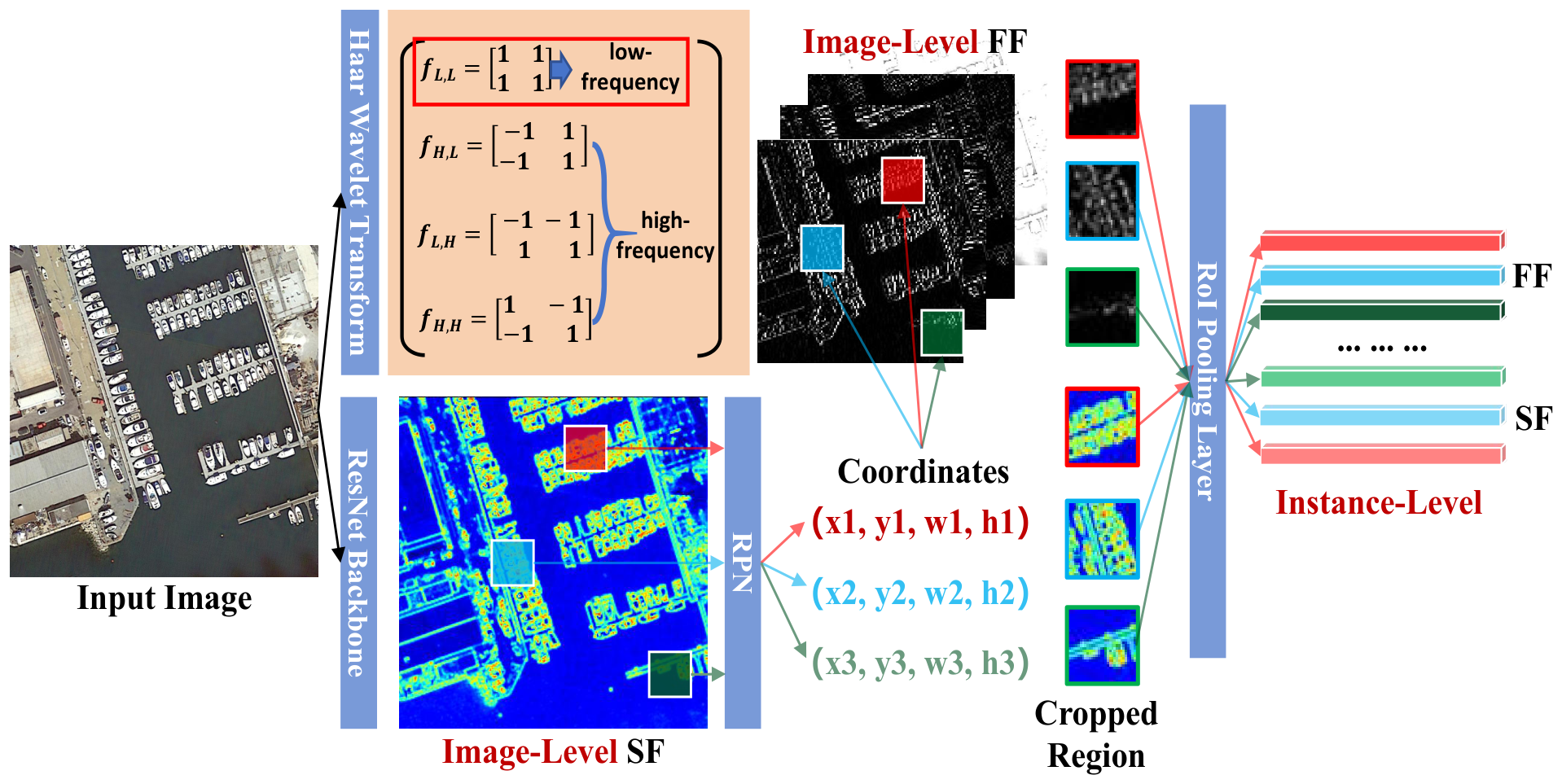
As illustrated in Figure 1, existing spatial–frequency fusion methods can be divided into two categories according to feature fusion granularity. The first category is image-level spatial–frequency fusion [9,10,11], which performs global fusion on the entire image. Global frequency features are extracted and fused with holistic CNN features to supplement angular prior. However, such fusion ignores local feature differences among individual target instances, leading to poor adaptability for rotated and multi-scale targets. The second category is instance-level spatial–frequency fusion [12,13], which constructs feature interaction within local region of interests (RoIs). However, this mechanism is vulnerable to complex background noise and semantic offset, resulting in severe false detection. Therefore, current spatial–frequency fusion detectors suffer from isolated fusion levels, insufficient information complementarity, and decoupled global–local representation, which cannot simultaneously guarantee global scene stability and local target accuracy.
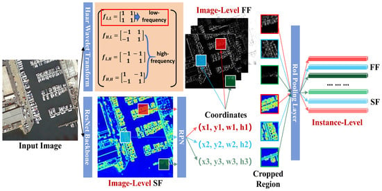
Figure 1.
Visualization of image-level and instance-level features. SF and FF denote the spatial feature and frequency feature, respectively. RPN denotes the region proposal network.
To address the aforementioned feature misalignment, this paper proposes a unified dual-level spatial–frequency collaborative detector termed DSCDet, which hierarchically integrates image-level global frequency prior injection and instance-level local geometric feature calibration into the detection pipeline. Specifically, the image-level branch exploits the directional selectivity of wavelet frequency sub-bands to compensate for the rotation-insensitive limitation of CNNs from a global perspective, while the instance-level branch constructs collaborative spatial–frequency weighting matrices on oriented RoIs to achieve fine-grained cross-domain feature alignment for small rotated targets. Moreover, a generic cross-domain attention fusion (GCDAF) module is constructed, which is customized to impose feature constraint rules for global scenes and local instances, respectively. This hierarchical collaborative fusion mechanism systematically alleviates the feature degradation of oriented targets at different granularities, which constitutes the core source of the consistent performance improvement.
From the perspective of feature representation, image-level and instance-level frequency modeling deliver complementary rather than redundant information. Image-level features correspond to 2D pyramid feature maps of size , which preserve global scene context, surrounding ground/object relations, and holistic frequency priors over the entire image. By contrast, instance-level features are obtained via RoI pooling layer on oriented candidate bounding boxes, producing feature vectors. Each vector encodes only the local content within a single target proposal and discards irrelevant background and inter-object context outside the bounding box. Consequently, joint dual-level frequency modeling aggregates two non-interchangeable sources of information instead of introducing redundant computations.
The main contributions of this paper are summarized as follows:
- A dual-level spatial–frequency collaborative detector (DSCDet) is proposed, which hierarchically integrates spatial–frequency calibration at both image and instance levels.
- A generic cross-domain attention fusion (GCDAF) module is developed. Global scene positional encoding and local instance pairwise positional encoding are designed for image-level and instance-level spatial–frequency feature fusion, respectively.
- Extensive experiments on DOTA-v1.0, DOTA-v1.5 and DIOR-R datasets verify that the proposed DSCDet achieves competitive accuracy against state-of-the-art OOD detectors.
2. Related Work
2.1. Oriented Object Detection for Remote Sensing Images
Remote sensing oriented object detection (OOD) aims to accurately localize and classify arbitrarily rotated targets [9,14,15]. Existing OOD approaches generally fall into three categories, including regression optimization, attention enhancement, and feature fusion. Regression optimization methods mitigate angle discontinuity and periodic mutation issues by refining rotated bounding box regression strategies. Typical schemes, such as circular smooth label (CSL) [16] and dense coding label (DCL) [17], effectively stabilize angle prediction but introduce heavy computational overhead from additional angular parameter fitting. Attention enhancement methods [18,19,20] highlight target discriminative features and suppress background noise. However, they rely purely on spatial information and lack explicit modeling of rotational deformation, leading to limited performance gains. Feature fusion methods exploit the complementarity of multi-type [13,21] features to break the representation limitation of single spatial features, which have dominated recent OOD research. Among various fusion strategies, spatial–frequency fusion exhibits unique superiority due to the inherent complementarity between spatial semantic texture and frequency deformation information. Nevertheless, existing spatial–frequency fusion methods rely on single-level fusion schemes, resulting in inadequate feature interaction and poor generalization in complex remote sensing scenarios.
2.2. Frequency-Aware and Multi-Scale Feature Refinement
The essential motivation of spatial–frequency fusion is to combine the semantic representation advantage of multi-scale CNN spatial features and the deformation perception advantage of frequency-domain features. Wavelet tree head attention (WTHA) [8] integrates the wavelet frequency tree structure with multi-head attention in the Transformer encoder to realize cross-interaction between short/long-range dependencies and frequency components. FDOL [9] introduces frequency-domain orientation awareness into the detection pipeline to enhance global angular representation, which utilizes the inherent directional selectivity of high-frequency sub-bands to model rotation-invariant features. Xu et al. [13] propose a multi-scale spatial–frequency network (MSFN) for OOD, which introduces multi-level Haar wavelet transforms to extract frequency-domain features and designs a channel-aligned feature fusion module to merge CNNs’ high-level semantic features with wavelet low-level texture features across multiple scales. Fu et al. [21] propose a frequency-assisted dynamic learning network (FADL-Net) to alleviate the crucial challenges for small object detection. They introduce a spatial–frequency feature pyramid network to adaptively capture global long-range feature representations.
Instance-level fusion methods conduct feature interaction within RoI regions. SFFD [12] extracts multi-scale instance-level frequency features and realizes cross-feature optimization, achieving significant improvement for detecting small and oriented objects. Ma et al. [22] address the instability of query-based detection from the instance-level perspective, and enhances instance feature representation via frequency-aware spatial modeling and density-guided query construction. Wang et al. [23] strengthen instance-level feature representation from the perspective of loss function, which extracts both domain-invariant spectrum and domain-specific spectrum for each target instance, so as to achieve more effective disentanglement of spectral features. Nevertheless, instance-level fusion completely discards global scene constraints. The lack of global semantic prior makes the detector susceptible to background clutter and pseudo-target interference, causing global semantic offset and extensive false detection.
2.3. Attention-Based Feature Interaction
Effective feature interaction between spatial and frequency domains is critical to fully unlock the complementary value of multi-domain features for OOD, and attention-based adaptive modeling has been extensively explored as a mainstream solution for precise feature interaction.
Self-attention [18] is the most widely adopted attention paradigm, which serves as the core building block of all Transformer-based feature interaction approaches [8,19,24,25,26,27,28]. For example, Wave-ViT [24] unifies wavelet transform and self-attention learning into a single framework, which replaces the conventional downsampling with invertible wavelet decomposition to preserve high-frequency texture details during feature reduction, achieving a better efficiency–accuracy trade-off while retaining complete frequency information. Pyramid vision Transformer (PVT) [25] presents a convolution-free Transformer backbone designed for dense prediction tasks and adopts a progressive shrinking pyramid structure to gradually reduce feature resolution. SpectFormer [19] leverages Fourier-based spectral gating to capture frequency-domain features in shallow layers, and applies self-attention for global semantic modeling in deeper layers, demonstrating that the fusion of frequency-domain prior and attention mechanism yields stronger visual representations.
Moreover, attention mechanisms under a CNN architecture present more diverse forms. SFFD [12] designs an orientation enhancement self-attention to realize attention-based spatial–frequency feature interaction. It leverages the inherent directional selectivity of high-frequency sub-bands, and applies adaptive attention weighting to selectively enhance features of oriented targets. CFIL [29] introduces a cross frequency-domain interaction learning scheme based on attention-guided feature fusion, which performs adaptive attention weighting and efficient fusion of spatial–frequency features across channels. DFGFNet [30] adopts a spatial-gated frequency attention mechanism to realize spatial–frequency feature enhancement. The proposed spatial-gated frequency attention module (SFAM) first employs a spatial gate to highlight salient target regions, then conducts local frequency calibration under the guidance of spatial attention weights, which amplifies orientation-relevant high-frequency components while suppressing irrelevant background frequency signals.
3. The Proposed Method
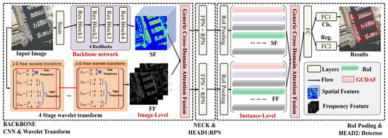
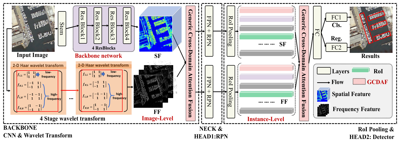
The overall architecture of our DSCDet is illustrated in Figure 2. Although deep CNNs embed implicit frequency information, such frequency cues are mostly preserved in shallow layers and degrade significantly as network depth increases. Shallow convolutions capture localization-relevant edges, contours and textures, whereas deep layers prioritize high-level semantic representations at the expense of fine-grained high-frequency geometric details. Our explicit multi-level Haar wavelet decomposition introduces two categories of complementary information unavailable from native CNN features. First, it persistently delivers sharp, well-localized edge and texture representations at each pyramid scale, counteracting the inherent high-frequency attenuation caused by stacked convolutions and supplying stable position priors for rotated bounding box regression. Second, the orthogonal high-frequency sub-bands yielded by wavelet transform explicitly decouple horizontal, vertical, and diagonal directional cues. The energy distribution over these sub-bands encodes physically interpretable orientation priors for arbitrarily rotated targets, mitigating CNNs’ intrinsic weakness in modeling rotation-invariant representations.
Figure 2.
The overall structure of our dual-level spatial–frequency collaborative detector (DSCDet). The DSCDet contains backbone, neck (FPN), head1 (RPN), RoI Pooling layer and head2 (detector) stages. The proposed generic cross-domain attention fusion (GCDAF) module is integrated into the backbone and detector stages. Cls. and Reg. represent the classification and regression branches, respectively.
3.1. Wavelet Transform for Frequency Feature Extraction
The two-dimensional Haar wavelet decomposition is implemented via four fixed 2 × 2 filters, which are formally defined as
where is the low-pass kernel that preserves smooth background and global object outline information. , and are directional high-pass kernels that encode horizontal, vertical and diagonal edge mutation features, respectively. These high-frequency detail components are inherently sensitive to target rotation and scale variation.
The four kernels defined in Equation (1) exactly form the filter bank of the Haar wavelet transform, and they are mathematically equivalent to the wavelet filters used in the following recursive decomposition process, satisfying , , , and . For an input image , the hierarchical wavelet decomposition is performed level by level. At each decomposition stage, the low-frequency approximation component from the previous level is convolved with the above four filter kernels, followed by 2 × downsampling, to generate four sub-band features of the current level. The recursive formulation is written as
where denotes the initial input. The operator ∗ denotes the convolution operator, and denotes the 2 × downsampling operation along both spatial dimensions. The variable s denotes the decomposition level index, corresponding to a downsampling factor of from the original input. is the low-frequency approximation component inherited from the -th decomposition level. For decomposition level s, the spatial resolution of the low-frequency approximation component as well as the three high-frequency sub-bands , , is . Each Haar wavelet decomposition level involves standard convolution and downsampling operations, yielding a computational complexity of per level, where H, W, and C denote the spatial and channel dimensions of the input.
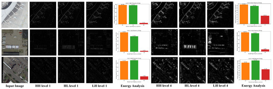
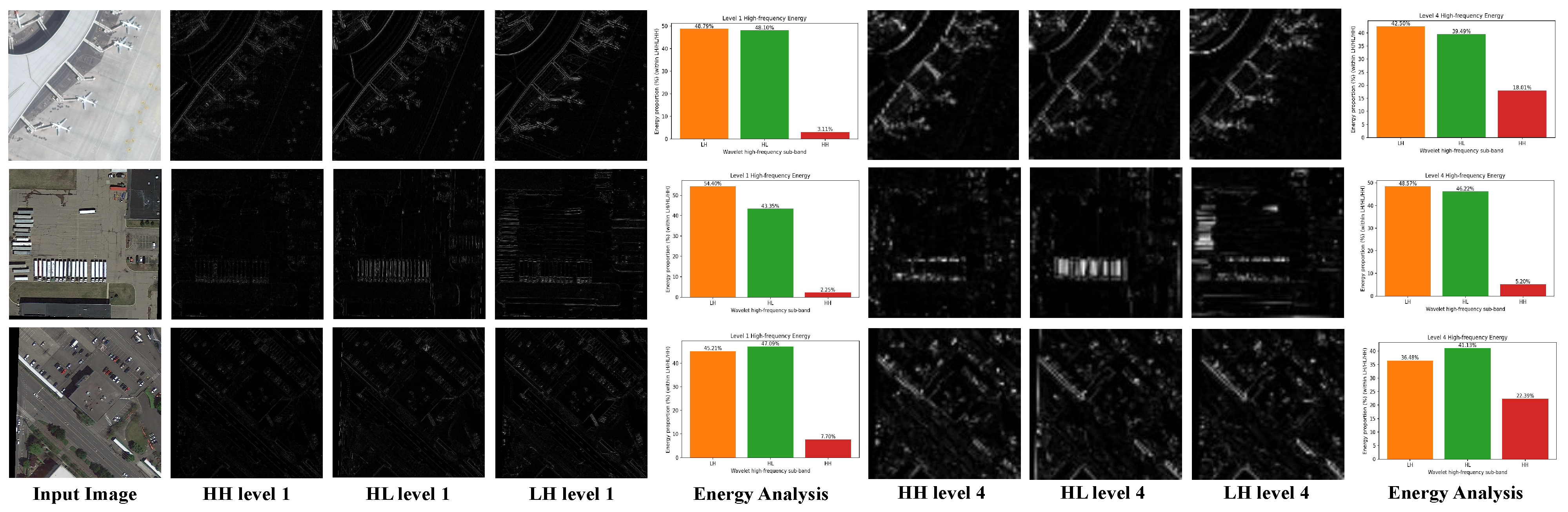
As illustrated in Figure 3, since the LL sub-band serves as the low-resolution approximation of the original signal and inherently dominates the overall energy, we discard LL and only analyze the normalized energy distribution among three high-frequency sub-bands LH, HL and HH. Three typical object categories are presented in different rows, including plane (PL), large-vehicle (LV), and small-vehicle (SV). PL and SV contains arbitrary orientations, while LV mainly exhibits strictly horizontal–vertical layouts. At level 1 decomposition, LH and HL carry much higher energy than the diagonal HH component for all samples, even for arbitrarily rotated PL and SV targets. As the decomposition goes to deeper levels, the HH sub band delivers more discriminative detail information, with the energy proportion of HH increasing noticeably for rotated PL and SV. In contrast, LV with axis aligned orientations maintains consistently low HH response across all decomposition levels. These observations verify the efficacy of our frequency-enhanced paradigm. Multi-level wavelet decomposition can compensate edge and contour details for large-resolution shallow CNN features, and additionally provide discriminative directional cues for small-resolution deep CNN features, which mitigates the loss of rotation-related geometric information caused by repeated convolution operation.
Figure 3.
Visualization of different wavelet sub-bands and corresponding normalized energy distribution for three typical categories, including PL, LV, and SV.
At each scale , the four decomposed frequency sub-bands are concatenated along the channel dimension to form the integrated frequency feature
The obtained multi-scale frequency feature set shares the same spatial resolution with the CNN pyramid feature set , laying the foundation for subsequent dual-granularity spatial–frequency fusion. Both and possess identical spatial dimension . In terms of channel dimension, , while the CNN pyramid features satisfy , , , and .
3.2. Generic Cross-Domain Attention Fusion (GCDAF)
We design a generic cross-domain attention fusion (GCDAF) scheme applicable to both image-level and instance-level, which constructs multi-type similarity weights combined with geometric positional prior to realize adaptive feature recalibration. The difference between image-level and instance-level fusion operation lies in the construction rule of , while the pipeline of attention calculation remains shared.
3.2.1. Feature Isomorphic Projection
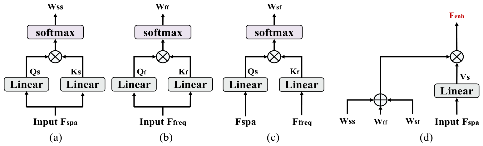
Spatial feature and frequency feature first pass independent projection layers to generate query, key, value matrices
where and are trainable projection weight matrices, introduced in self-attention mechanism [18].
3.2.2. Tripartite Similarity Weight Calculation
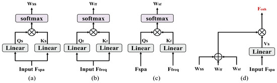
As illustrated in Figure 4, three categories of scaled dot-product similarity matrices are computed to model intra-spatial, intra-frequency, cross spatial–frequency feature correlations
where denote the dimensions of key vectors in each corresponding attention branch, and the square-root scaling term is adopted to normalize the magnitude of dot-product values, preventing the softmax function from entering the saturation region and alleviating gradient vanishing. For the instance-level branch, let N be the number of RoI features and the three similarity matrices satisfy . The pairwise dot-product computation for each matrix yields a complexity of , where denotes the dimension of key vectors. For the image-level branch upon dense feature maps, let be the total number of flattened spatial tokens of the feature map with spatial size , then satisfies . Correspondingly, the computational complexity for each similarity matrix under image-level is .
Figure 4.
Visualizations of our proposed generic cross-domain attention fusion (GCDAF) module. Given the input spatial and frequency features , the final enhanced feature is obtained by sequentially performing operations (a–d). The linear function is employed for instance-level GCDAF, while the image-level GCDAF is modified and implemented via convolutional layer.
3.2.3. Geometric Positional Weight Calibration
Followed by the standard self-attention algorithm [18], is further embedded as
where i denotes the channel dimension index of the position embedding, d represents the total dimension of the embedding vector, and denotes the normalized spatial position coordinates of input features. This parameter-free encoding scheme constructs unique position representations for each spatial location via sine and cosine functions with progressively decreasing frequencies, which endows the model with inherent relative position perception capability without introducing additional trainable parameters.
The embedded positional tensor is compressed through convolution and reshape operations to generate normalized geometric weight . Each similarity matrix is calibrated as
where ⊙ denotes Hadamard element-wise product, and performs summation along feature dimension for normalization.
3.2.4. Comprehensive Fusion Weight for Feature Refinement
The weighted summation of three calibrated correlation matrices (Equation (7)) yields the final attention-weight matrix as
This formulation can be interpreted as the closed-form solution of a regularized least-squares feature-alignment optimization objective , where the regularization term encodes the prior that optimal should be a composite of three correlation components and . Rather than iteratively solving this objective, our network learns the coefficients and end-to-end via back-propagation to implicitly approximate its optimal solution. The enhanced spatial feature is calculated as
For the instance-level branch, we have . The fused weight matrix , and the enhanced output feature satisfies . The matrix-multiplication operation brings computational complexity . For the image-level branch, let denote the number of flattened tokens from feature map and C denote the channel dimension. , , and the output enhanced feature is , which is further reshaped as . The corresponding matrix multiplication complexity is . The above pipeline forms a plug-and-play universal fusion core. We deploy it on image-level global feature maps and instance-level RoI feature vectors separately, and the only variable is the construction formula of .
3.3. Dual-Level Spatial–Frequency Collaborative Detector
3.3.1. Image-Level Global Spatial–Frequency Fusion
Image-level fusion takes spatial and frequency feature maps of the entire image as input, aiming to build global scene spatial–frequency constraints and suppress background noise.
- (1)
- Global Positional Feature Construction
Taking the center coordinate of the whole feature map as reference, for any pixel coordinate on the feature map with width W and height H, we construct the global positional feature to encode relative spatial geometric information. To avoid numerical undefinedness caused by when the pixel coincides exactly with the reference center, we introduce a tiny positive numerical stabilizer to clamp the coordinate offset before the logarithm operation. The formal definition is written as
where the first two terms encode the normalized horizontal and vertical relative offsets of each pixel with respect to the feature map center. These spatially varying components provide position-aware geometric cues for attention calculation. The last term is a global constant independent of pixel positions, which preserves the overall aspect ratio information of the current feature scale and serves as a supplementary scale prior. Finally, we feed into the embedding function (Section 3.2.3) to obtain the global geometric weight .
- (2)
- Global Fusion Execution
The paired multi-scale spatial feature and frequency feature , together with the global geometric weight , are fed into the GCDAF module to produce globally enhanced feature maps . All multi-scale enhanced features are assembled into a feature pyramid and delivered to the region proposal network (RPN) for generating rotated candidate proposals , which supply global angular priors to the subsequent instance-level processing stage.
3.3.2. Instance-Level Local Spatial–Frequency Fusion
- (1)
- RoI Feature Alignment
All multi-scale spatial pyramids and frequency pyramids are sent into RoI pooling layer [7] with identical proposal set . A fully-connected layer unifies channel dimensions of frequency RoI feature and spatial RoI feature
Both , where N denotes the number of RoI instances, and d denotes unified feature dimension.
- (2)
- Instance Pairwise Positional Feature Construction
For any two RoIs a and b with center coordinates and bounding box sizes , we construct the pairwise relative positional representation. Specifically, RoI a acts as the query, and all coordinate offsets and scale ratios are normalized by the size of the query RoI a. The numerical stabilizer is adopted to guarantee numerical stability. The aforementioned operation is defined as
where records the relative offset and scale ratio between arbitrary instance pairs.
Moreover, this pairwise positional encoding is asymmetric, i.e., . Equality holds only when the two RoIs have exactly identical center coordinates and exactly the same width and height. For diagonal self-pairs where an RoI is paired with itself, we follow the native self-attention paradigm [18] and do not apply additional masking. The diagonal elements naturally participate in feature recalibration and are automatically learned by the model under task supervision, and they remain numerically stable with the clamping stabilizer. It is worth noting that even when two RoIs share the same center, the scale ratio terms can still provide distinguishable features as long as their sizes differ, which effectively alleviates the feature indistinguishability caused by center coincidence. We also feed into the embedding function, proposed in Section 3.2.3, to generate the instance geometric weight .
- (3)
- Instance Feature Refinement
Scalability of the instance-level GCDAF is bounded by the number of input RoIs N. Since pairwise correlation computation yields computational and memory complexity, naive implementation would suffer quadratic growth for dense scenes with abundant small objects. In our pipeline, the proposal sampler fixes the maximum number of RoIs fed into GCDAF to 512 (the default setting in most OOD methods) by retaining only top-scoring candidates, which constrains the practical overhead and avoids complexity explosion. We further profile GPU memory and training latency under different RoI numbers N on a single GTX 1080ti GPU. While moderate overhead is observed for , out-of-memory errors occur when , revealing the upper-bound limitation of the instance-level pairwise fusion for extremely heavy proposal counts.
Here, we feed into the GCDAF module to output refined instance feature . Finally, is delivered to final classification head and rotated bounding box regression head for oriented object detection
where denotes the predicted category logits, and represents the five-parameter rotated bounding box prediction, containing center coordinates, width, height and rotated angle.
4. Experiments
4.1. Datasets and Evaluation Metrics
Extensive experiments are conducted on three OOD datasets, including DOTA-v1.0, DOTA-v1.5 and DIOR-R, to evaluate the effectiveness and generalization of the proposed DSCDet.
(1) DOTA-v1.0: DOTA is a large-scale aerial OOD dataset, containing 2806 high-resolution images and 15 categories with arbitrary rotation and drastic scale variation. Following standard experimental protocols, the training and validation subsets are utilized for training, and the test subset for performance evaluation. Fifteen categories contain plane (PL), baseball diamond (BD), bridge (BR), ground track field (GTF), small-vehicle (SV), large-vehicle (LV), ship (SH), tennis court (TC), basketball court (BC), storage tank (ST), soccer-ball field (SBF), roundabout (RA), harbor (HA), swimming pool (SP), and helicopter (HC). Input images are cropped into patches with a 200 pixels overlapping region. Our model is trained for 12 epochs with an SGD optimizer, a batch size of 1, an initial learning rate of 0.005, and a step learning rate decay at 8 and 11 epochs.
(2) DOTA-v1.5: Compared to DOTA-v1.0, DOTA-v1.5 contains a new category, named container crane (CC). Furthermore, a total of 402,089 instances are labeled in DOTA-v1.5, which is more difficult than DOTA-v1.0. Importantly, our method is also trained for 12 epochs with SGD optimizer, a batch size of 1, an initial learning rate of 0.005, and a step learning rate decay at 8 and 11 epochs.
(3) DIOR-R: DIOR-R is a challenging large-scale rotated remote sensing dataset covering 20 categories with complex background interference. The dataset contains 23,463 images with diverse spatial resolutions and rotation angles, which is adopted to verify the complex scene generalization capability of the proposed method. The training, validation, and test split follows official standard settings.
All experiments are implemented on the PyTorch 3.13.9 framework with one NVIDIA GTX 1080ti GPU. Mean Average Precision (mAP) under Pascal VOC 2007/2012 criteria [7] and COCO-style AP metrics [31] are adopted for comprehensive quantitative evaluation.
4.2. Performance Evaluation
4.2.1. DOTA-v1.0
As listed in Table 1, comprehensive quantitative comparisons on the DOTA-v1.0 benchmark validate the superiority of our proposed DSCDet over state-of-the-art oriented detectors. In terms of overall mAP metric, our method reaches 78.28%, which surpasses the ViT-based DynaPro (77.85%) by 0.43% and the LSKNet-S model (77.49%) by 0.79%, respectively. For fine-grained per-category performance, DSCDet achieves the best and second-best accuracy on five challenging classes. Among them, BR comprises long, strip-shaped objects with extreme aspect ratios that easily suffer feature blurring and angle aliasing. The consistent performance gain originates from the dual-level spatial–frequency collaborative fusion design, where the image-level wavelet frequency module extracts global directional edge priors to compensate CNN rotation-insensitive defects, and the instance-level cross-fusion module models pairwise geometric constraints to eliminate feature confusion of elongated targets. Moreover, different from existing single-granularity spatial–frequency collaborative method FDOL [9] that only exploit image-level feature relations, our dual-level unified framework simultaneously captures global scene angular context and local instance geometric correlation, which explains the consistent accuracy boost across most complex categories.
Table 1.
Quantitative comparisons of various detection algorithms on the DOTA-v1.0 benchmark. Here, BB stands for the adopted backbone architecture. * denotes the multi-scale training and testing strategy. All comparative experimental data are reproduced using the publicly released source codes of corresponding approaches. The optimal and suboptimal mAP values for each target category are marked in bold with colored background and underlined format, respectively.
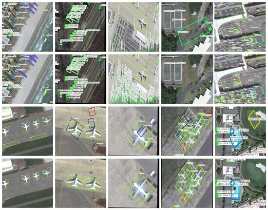
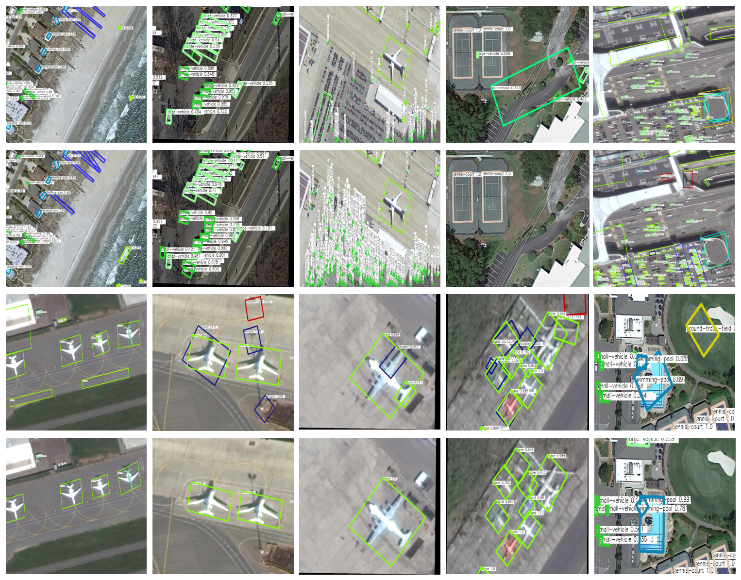
Figure 5 presents qualitative detection comparisons on the DOTA dataset. In this visualization diagram, odd rows illustrate prediction results generated by the baseline ARC detector, whereas even rows visualize the outputs produced by our DSCDet method. Intuitive visual contrast reveals the prominent advantages of the proposed dual-level spatial–frequency fusion framework. Benefiting from the collaborative modeling of global frequency priors and instance geometric constraints, our DSCDet successfully retrieves the rotated targets, and produces compact oriented bounding boxes that fit the actual contours of arbitrarily rotated objects more precisely.
Figure 5.
Visualizations of different methods on the DOTA dataset. Odd rows display detection outputs from the baseline model, while even rows correspond to the predictions yielded by our proposed DSCDet.
4.2.2. DOTA-v1.5
Table 2 presents comprehensive quantitative comparisons of single-scale oriented detection methods on the DOTA-v1.5 dataset, which introduces an extra container crane (CC) category with scarce training samples. In terms of overall mAP, our proposed DSCDet reaches 70.95%, outperforming the second-best SOOD model (70.39%) by 0.56% and the LSKNet-S baseline (70.26%) by 0.69%. From the perspective of per-category detection accuracy, DSCDet achieves best and second-best performance on five target categories. Existing mainstream detectors only exploit spatial features or single-granularity spatial–frequency interaction. Our DSCDet simultaneously models global scene frequency constraints and local instance geometric correlations, which jointly enhance the discriminability of rotated targets with arbitrary scales, and yields the optimal overall detection accuracy on the DOTA-v1.5.
Table 2.
Quantitative comparisons of various detection algorithms on the DOTA-v1.5 benchmark. All comparative experimental data are reproduced using the publicly released source codes of corresponding approaches. The optimal and suboptimal mAP values for each target category are marked in bold with colored background and underlined format, respectively.
4.2.3. DIOR-R
Table 3 reports the quantitative comparisons of mainstream oriented detectors on the DIOR-R dataset, which contains 20 diverse categories. In terms of overall mAP metric, our proposed DSCDet reaches 68.13%, which outperforms the second-best RQFormer (67.31%) by a 0.82%, which fully demonstrates the superiority of our unified dual-level spatial–frequency fusion architecture. In terms of per-category detection accuracy, DSCDet achieves the best and second-best AP on eight representative difficult categories. For small targets such as SH and ESA, which are easily submerged in complex background, the instance-level pairwise geometric positional encoding module strengthens the frequency feature response of small objects, effectively alleviating small-object-feature attenuation.
Table 3.
Quantitative comparison of various detection algorithms on the DIOR-R benchmark. All comparative experimental data are reproduced using the publicly released source codes of corresponding approaches. The optimal and suboptimal mAP values for each target category are marked in bold with colored background and underlined format, respectively.
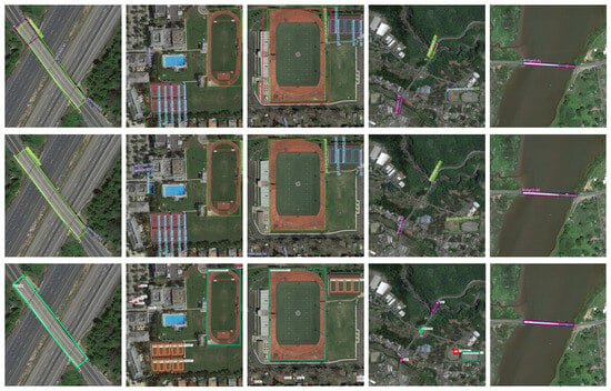
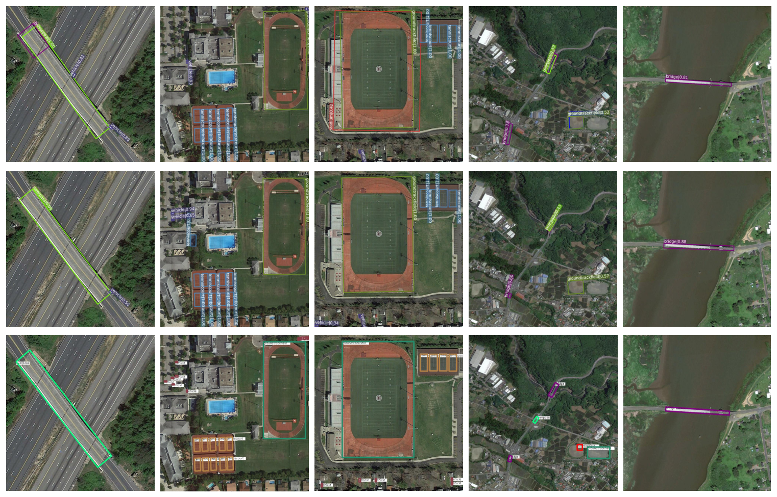
Figure 6 presents qualitative detection comparisons on the DIOR-R dataset. It can be clearly seen that our DSCDet successfully detects more small targets, which better fits the actual contours of arbitrarily rotated objects.
Figure 6.
Visualizations of different methods on the DIOR-R dataset. The first and second rows show the detection results of baseline method and our proposed DSCDet. The third row shows the visualizations of the ground truth.
4.3. Ablation Study
4.3.1. Image-Level Branch
- (1)
- Comparisons with Different Frequency-Analysis Tools
As listed in Table 4, all frequency-domain operators, including FFT, DCT and different wavelet families, are fixed mathematical transforms without trainable parameters, so all variants share nearly identical parameters, which sufficiently verifies that the performance gain of our method comes from genuine spatial–frequency feature complementarity rather than additional learnable parameters. In terms of computational cost, the FLOPs show minor differences, which is mainly determined by the inherent transform mechanisms. Wavelet-based methods with linear complexity have lower overhead than global transforms with FFT complexity.
Table 4.
Quantitative results of our image-level GCDAF with different frequency tools on the DOTA-v1.0 benchmark. Parameters (M), FLOPs (G), mAP75 and mAP50 are used for evaluation.
For detection accuracy, the Haar wavelet with the most compact support maintains the best spatial localization of edge, corner and fine texture details, providing the strongest complementary effect for CNN semantic features. In contrast, Daubechies and Symlets with better smoothness slightly blurs local details achieve sub-optimal performance, as the loss of fine-grained details outweighs the benefit of smoothness in remote sensing scenes dominated by small targets. DCT outperforms FFT thanks to its better energy compaction of real-valued transform, while global FFT with poor spatial localization brings limited complementary gain and even slight performance fluctuation on strong baselines. Overall, the Haar wavelet achieves the optimal balance of accuracy, efficiency and implementation simplicity, making it the most suitable frequency-domain operator for our dual-granularity spatial–frequency fusion framework.
- (2)
- Influence of LL, HL, LH, HH Bands
As shown in Table 5, the full combination of all four frequency sub-bands achieves the best detection performance, verifying the complementarity of frequency components with different directional characteristics. The removal-based strategy clearly quantifies the contribution of each sub-band. Specifically, removing the HH diagonal high-frequency sub-band leads to the most significant accuracy drop, indicating that diagonal edge and fine texture details are the most critical complementary information for oriented remote sensing targets. Dropping LH or HL high-frequency sub-band causes moderate performance degradation with comparable contribution, corresponding to horizontal and vertical structural features respectively. In contrast, the LL low-frequency approximation sub-band only results in a tiny accuracy decline, since the CNN backbone has already captured sufficient low-frequency contour and semantic information, and the gain of the frequency-domain branch mainly comes from high-frequency directional details.
Table 5.
Ablation study on frequency sub-bands of the image-level GCDAF on the DOTA-v1.0 benchmark. We adopt the removal-based strategy to quantify the contribution of each sub-band.
- (3)
- Influence of , , and
Table 6 illustrates the individual and combined contributions of three attention weights under two different baseline frameworks. Adding only corresponds to pure spatial self-attention, which models long-range semantic dependencies within spatial features and brings limited accuracy improvement. Introducing the cross-domain weight further exploits directional frequency priors to calibrate spatial feature distribution, which effectively compensates for the rotation-insensitive defect of CNNs and yields more noticeable performance gains.
Table 6.
Influence of , , and in our proposed image-level GCDAF with different baseline methods on the DOTA-v1.0 benchmark. mAP75 and mAP50 are used for evaluation.
Importantly, activating only the frequency self-correlation weight delivers no obvious accuracy improvement and only presents minor performance fluctuations. The underlying mechanism is that only models the internal structural correlation within frequency-domain features. Since it neither carries spatial semantic information nor builds cross-domain feature mapping relationships, it cannot provide effective semantic enhancement. When , and are activated simultaneously, the model fully integrates spatial self-correlation, spatial–frequency cross correlation and frequency self-correlation for joint feature enhancement. Under both ReDet and ARC baselines, this complete combination achieves the highest mAP50 and strict mAP75, demonstrating that the three collaborative weight matrices jointly exploit complementary spatial and frequency domain information and deliver optimal detection performance.
4.3.2. Instance-Level Branch
- (1)
- Comparisons with Different Frequency-Analysis Tools
As listed in Table 7, consistent with the image-level results, the instance-level GCDAF also follows highly similar patterns in parameter complexity, computational cost and detection performance across different frequency tools, which further verifies the generality of our spatial–frequency complementary mechanism. In terms of detection accuracy, the Haar wavelet consistently achieves the best performance on both backbones, since instance-level detection relies more on precise edge and corner localization for oriented RoI feature enhancement, and the compact support of the Haar wavelet best preserves fine-grained directional details of each proposal. Daubechies and Symlets obtain slightly lower accuracy due to their longer filters that partially blur local details, while DCT and FFT with weaker spatial localization bring limited performance gain.
Table 7.
Quantitative results of our instance-level GCDAF with different frequency tools on the DOTA-v1.0 benchmark. Parameters (M), FLOPs (G), mAP75 and mAP50 are used for evaluation.
- (2)
- Influence of LL, HL, LH, and HH Bands
Consistent with the image-level ablation, the instance-level GCDAF follows the same sub-band contribution pattern, further verifying the universality of our spatial–frequency complementary mechanism across different feature granularities. As listed in Table 8, the full combination of all four sub-bands achieves the best detection performance, proving that multi-directional frequency components cooperatively enhance instance-level feature representation. Removing the HH diagonal high-frequency sub-band causes the largest accuracy drop, as instance-level oriented detection and pairwise relation modeling depend heavily on precise corner localization and oblique texture details for accurate bounding box regression and instance similarity measurement. All variants share nearly identical parameter counts and computational overhead with no extra complexity burden. These results consistently confirm that directional high-frequency components are the core source of performance gain for both the image-level and instance-level fusion modules.
Table 8.
Ablation study on frequency sub-bands of the instance-level GCDAF on the DOTA-v1.0 benchmark. We adopt the removal-based strategy to quantify the contribution of each sub-band.
- (3)
- Influence of , , and
As listed in Table 9, three weight matrices play distinct roles on instance RoI features. Only adopting spatial self-weight corresponds to standard SE attention with limited gains. Adding cross-domain weight introduces local frequency cues between instances and brings larger accuracy improvement. When , and work collaboratively, the model simultaneously models intra-spatial, spatial–frequency and intra-frequency correlations of object instances, yielding the highest mAP50 and strict mAP75 for both backbones.
Table 9.
Influence of , , and in our proposed instance-level GCDAF with different baseline methods on the DOTA-v1.0 benchmark. mAP75 and mAP50 are used for evaluation.
4.3.3. Influence of Image and Instance-Level Branches
- (1)
- Gains of Image-Level and Instance-Level Branches
Table 10 compares the independent and combined contributions of the two proposed branches. The image-level module brings slight computation overhead and moderate performance improvement by extracting global directional frequency priors. In contrast, the instance-level branch introduces more parameters and FLOPs but achieves larger gains on strict mAP75 criterion, as it suppresses feature confusion among rotated objects via local pairwise geometric constraints. When both branches are integrated, the model combines global scene frequency context and local instance feature interaction simultaneously, reaching the optimal overall mAP50 and the highest mAP75 on the ARC backbone. This result demonstrates that the two branches are complementary and jointly promote detection accuracy for arbitrarily oriented targets in RSIs.
Table 10.
Gains of image-level and instance-level GCDAF in our method on the DOTA-v1.0 benchmark. Parameters (M), FLOPs (G), mAP75 and mAP50 are used for evaluation.
- (2)
- Influence of Different Fusion Coefficient Strategies for , and
From the results in Table 11, the fixed equal weight and learnable fusion strategies achieve consistent and significant performance improvement over different backbone networks, while the normalized fusion strategy obtains limited accuracy gain and even causes slight performance degradation under the weaker ReR50 backbone. The underlying reason is that the normalized strategy generates adaptive fusion weights purely based on channel-wise feature energy via softmax, which inherently suppresses high-frequency sub-bands with lower energy amplitude. The best performances (78.15% and 78.28% mAP50), under different backbone networks, are achieved by the learnable fusion strategy, which fine-tunes the fusion weights to better fit the dataset distribution, achieving comparable overall performance with a marginal improvement in mAP50.
Table 11.
Influence of different fusion coefficient strategies for , , and in our DSCDet. ReR50 and ARC50 backbones are adopted, and mAP75 & mAP50 are used for evaluation.
- (3)
- Comparison with Other Spatial–Frequency Fusion and Attention Interaction Methods
Table 12 summarizes the performance comparison with spatial–frequency fusion and attention interaction methods, covering both CNN and Transformer detection architectures. Most spatial–frequency fusion methods exploit multi-level frequency transformation to supplement texture details for spatially small targets, which is proven effective to alleviate feature degradation of small objects during downsampling. Transformer-based schemes such as WaveViT [24] and SpectFormer [19] integrate frequency priors into self-attention modeling to capture multi-scale long-range dependencies, achieving 76.40% and 76.03% mAP50, respectively. However, their heavy backbone architectures usually bring huge parameters and computational overheads, which raise high requirements for deployment hardware. The CNN-based counterpart FADL-Net [21] focuses on small target optimization with lighter frequency enhancement structures and yields 74.80% mAP50. However, the single-granularity global fusion always limits its final accuracy gain.
Table 12.
Comparisons between other spatial–frequency feature fusion and attention-based feature interaction methods. CNN- and Transformer-based [27] approaches are involved for comparison.
For attention-based feature interaction methods, various attention operators are adopted to realize adaptive spatial–frequency feature fusion. FDOL [9] injects orientation-aware frequency priors via spectral attention layers to enhance global angular representation, achieving 77.22% mAP50. DFGFNet [30] further introduces spatial-gated frequency attention to suppress background interference, reaching 77.75% mAP50 with relatively moderate model complexity. Nevertheless, most of schemes perform feature interaction only at the image-level feature pyramid, without establishing fine-grained frequency enhancement at the instance-level, which restricts accuracy improvement for rotated and small targets.
- (4)
- Accuracy–Complexity Trade-Off Among Different Methods
As presented in Table 13, we systematically compare the accuracy–complexity trade-off of different detection methods under strictly controlled variables. All methods are built on the ReDet baseline with ReR50 backbone, and the efficiency metrics are measured on a single NVIDIA GTX 1080ti GPU to ensure fair comparison. Our proposed DSCDet achieves the highest detection accuracy of 78.14% mAP50 among all compared schemes, verifying the effectiveness of our dual-granularity spatial–frequency collaborative enhancement framework. FDOL [9] and SFFD [12] also introduce frequency-domain orientation awareness to enhance angular representation, but they only exploit frequency features at single-feature granularity, resulting in limited feature discrimination. MAC [67] achieves competitive detection accuracy, but its complex module structures bring drastically increased FLOPs and training time (246.59 G and 46.2 h). Moreover, the mAP50 of our method is the average result over three independent training runs with different random seeds, and the standard deviation is provided to quantify performance stability. Since the frequency decomposition is a parameter-free and deterministic transformation, the extracted multi-band frequency features for the same input image remains completely consistent across different training runs, and introduce no additional randomness into the feature extraction pipeline. The minor performance fluctuation 0.07% mainly originates from the stochastic characteristics of the CNN detection pipeline, including random weight initialization of the backbone network and detection head, and random data augmentation during training.
Table 13.
Accuracy–complexity trade-off comparisons of different methods on the DOTA-v1.0 benchmark. All methods are built on the ReDet baseline with ReR50 backbone, and the resolution of input sample is fixed as 1024 × 1024. All efficiency metrics are measured on a single NVIDIA GTX 1080ti GPU. Our method is trained three times with different random seeds, and we report the mean and standard deviation of mAP.
It is important to note that our DSCDet introduces non-negligible complexity increment, bringing certain growth in parameters, FLOPs, training times and inference FPS, and there remains room for optimization to satisfy the requirements of resource-constrained edge deployment. In future work, we will further streamline the computation pipeline of wavelet feature fusion and explore more lightweight dual-granularity interaction patterns to further compress model overhead and improve inference efficiency while preserving the accuracy gain.
5. Discussion
5.1. Limitations
Although DSCDet achieves competitive detection performance on public optical remote sensing benchmarks, there still exist inherent limitations that deserve further discussion. First, from the perspective of computational efficiency, the introduction of wavelet-based frequency decomposition and instance-level cross-domain feature interaction inevitably increases the overall parameters and inference latency. The additional computational overhead restricts its direct deployment on resource-limited edge airborne platforms. Second, the wavelet frequency enhancement mechanism effectively compensates for the missing edge and texture details of small and arbitrarily oriented targets in CNNs. However, it simultaneously strengthens high-frequency background textures and noisy interference that are naturally suppressed by conventional CNNs. Future work will focus on designing adaptive frequency filtering and background suppression modules to retain target-sensitive geometric priors while inhibiting irrelevant high-frequency noise. Third, the current validation is mainly conducted on optical remote sensing datasets, and the general performance of the proposed spatial–frequency collaborative paradigm across different modalities such as SAR and hyperspectral imagery has yet to be fully verified. The universal applicability of frequency-domain prior knowledge under different imaging mechanisms remains to be further explored.
5.2. Implications of Dual-Level Spatial–Frequency Collaborative Modeling
The experimental results of DSCDet further verify that frequency-domain information serves as an effective complement to spatial features for OOD in RSIs, and the dual-level collaborative fusion paradigm can fully unleash the complementary value of multi-domain features. Different from single-level global frequency enhancement methods, the combination of image-level global frequency prior injection and instance-level local feature calibration naturally matches the two-stage detection pipeline, where the image-level branch compensates for the rotation-insensitive defect of convolutional downsampling, and the instance-level branch performs targeted frequency refinement on candidate regions to suppress missing detection caused by feature aliasing of small targets.
6. Conclusions
In this paper, we propose a dual-level spatial–frequency collaborative detector (DSCDet) for oriented object detection in remote sensing images. Different from existing methods that only perform feature learning on a single-granularity spatial or frequency domain, the proposed framework integrates image-level global frequency enhancement and instance-level local feature optimization to comprehensively tackle the detection challenges caused by arbitrary object orientations and small target resolutions. On the image-level branch, wavelet frequency analysis is leveraged to capture directional edge and contour priors, which effectively compensates for the rotation-insensitive limitation of standard CNNs. On the instance-level branch, collaborative spatial–frequency weighting matrices are constructed to model the spatial self-correlation, cross-domain interaction and frequency self-correlation of oriented RoIs, which alleviates feature confusion among rotated and small targets.
While the proposed framework yields favorable detection performance on public benchmarks, there remain multiple promising directions to further improve its practical applicability and generalizability for real-world remote sensing applications: (1) image quality enhancement modules, such as super-resolution networks can be introduced to pre-process degraded remote sensing imagery, and the inherent anti-interference property of frequency-domain features will be further exploited to mitigate performance degradation under complex meteorological conditions; (2) lightweight optimization of the spatial–frequency collaborative pipeline can be further explored, where more efficient cross-domain feature interaction operators and model compression strategies can be adopted to reduce parameter and computational complexity; and (3) multi-source remote sensing data, such as SAR and hyperspectral images, can be integrated into the framework to investigate the generalizable value of frequency-domain prior-knowledge across different sensing modalities.
Author Contributions
Conceptualization, X.S., S.Z.; methodology, X.S.; software, J.S.; validation, X.S. and J.S.; formal analysis, Z.W.; investigation, X.S. and S.Z.; resources, S.Z.; data curation, X.S., J.S., and K.Y.; writing—original draft preparation, X.S. and J.S.; writing—review and editing, S.Z. and K.Y.; visualization, J.S. and K.Y.; supervision, S.Z.; project administration, S.Z.; funding acquisition, S.Z. All authors have read and agreed to the published version of the manuscript.
Funding
This work was supported in part by the National Natural Science Foundation of China, under Grant 62401277, Grant 62402231, Grant U23B2006, Grant 92370203, Grant 62071233, and Grant 61802202; in part by the Basic Research Program of Jiangsu, under Grant BK20240624; in part by the Jiangsu Province Youth Science and Technology Talent Support Project, under Grant JSTJ-2025-135; in part by the Jiangsu Provincial Innovation Support Program, under Grant BZ2023046; in part by the Jiangsu Provincial Key Research and Development Program, under Grant BE2022065-2; in part by the Jiangsu Provincial Natural Science Foundation of China, under Grant BK20211570; in part by the Natural Science Research Start-up Foundation of Recruiting Talents of Nanjing University of Posts and Telecommunications, under Grant NY224029; and in part by the Natural Science Foundation for Colleges and Universities in Jiangsu Province, under Grant 23KJB520026.
Institutional Review Board Statement
The study did not involve humans or animals.
Informed Consent Statement
The study did not involve humans.
Data Availability Statement
The datasets in this study are available online from https://captain-whu.github.io/DOTA/dataset.html (accessed on 19 August 2026) and https://aistudio.baidu.com/datasetdetail/123364 (accessed on 19 August 2026).
Acknowledgments
The authors would like to thank the NVIDIA Corporation (Santa Clara and United States) for their support in providing the GTX 1080ti GPU used in this research.
Conflicts of Interest
The authors declare no conflicts of interest. The funders had no role in the design of the study; in the collection, analyses, or interpretation of data; in the writing of the manuscript; or in the decision to publish the results.
References
- Yu, Y.; Da, F. Phase-shifting coder: Predicting accurate orientation in oriented object detection. In Proceedings of the IEEE/CVF Conference on Computer Vision and Pattern Recognition; IEEE: Piscataway, NJ, USA, 2023; pp. 13354–13363. [Google Scholar]
- Yuan, H.; Zhang, B.; Wang, Y.; Qiang, Q. From Structural Degradation to Semantic Misalignment: A Unified Frequency-Aware Compensation Framework for Remote Sensing Object Detection. Remote Sens. 2026, 18, 777. [Google Scholar] [CrossRef] [Scilit]
- Khan, M.R.K.; Rishe, N. A unified framework for vehicle detection, tracking, and counting across ground and aerial views using knowledge distillation with YOLOv10-S. Remote Sens. 2026, 18, 842. [Google Scholar] [CrossRef] [Scilit]
- Wang, Q.; Sun, W. A Dual-Branch Perception Network for High-Precision Oriented Object Detection in Remote Sensing. Remote Sens. 2026, 18, 839. [Google Scholar] [CrossRef] [Scilit]
- Liu, D.; Ying, X.; Liu, Z.; Peng, Y.; Gao, S.; Guo, F. VODet: A Vertex Offset-Based Method for Oriented Object Detection in Remote Sensing Images. Remote Sens. 2026, 18, 2296. [Google Scholar] [CrossRef] [Scilit]
- Wang, G.; Lu, Z.; Chen, J. SFPNet: Self-Learning Small Object Detection for Large-Scale Remote Sensing Images. IEEE J. Sel. Top. Appl. Earth Obs. Remote Sens. 2026, 19, 3290–3301. [Google Scholar] [CrossRef] [Scilit]
- Ren, S.; He, K.; Girshick, R.; Sun, J. Faster R-CNN: Towards Real-Time Object Detection with Region Proposal Networks. IEEE Trans. Pattern Anal. Mach. Intell. 2017, 39, 1137–1149. [Google Scholar] [CrossRef] [Scilit] [PubMed]
- Pan, J.; He, C.; Huang, W.; Cao, J.; Tong, M. Wavelet tree transformer: Multihead attention with frequency-selective representation and interaction for remote sensing object detection. IEEE Trans. Geosci. Remote Sens. 2024, 62, 5637023. [Google Scholar] [CrossRef] [Scilit]
- Zheng, S.; Wu, Z.; Xu, Y.; Wei, Z.; Plaza, A. Learning Orientation Information From Frequency-Domain for Oriented Object Detection in Remote Sensing Images. IEEE Trans. Geosci. Remote Sens. 2022, 60, 5628512. [Google Scholar] [CrossRef] [Scilit]
- Zhao, J.; Ding, Z.; Zhou, Y.; Zhu, H.; Du, W.L.; Yao, R.; El Saddik, A. RQFormer: Rotated Query Transformer for end-to-end oriented object detection. Expert Syst. Appl. 2025, 266, 126034. [Google Scholar] [CrossRef] [Scilit]
- Zhao, J.; Ding, Z.; Zhou, Y.; Zhu, H.; Du, W.L.; Yao, R.; El Saddik, A. OrientedFormer: An End-to-End Transformer-Based Oriented Object Detector in Remote Sensing Images. IEEE Trans. Geosci. Remote Sens. 2024, 62, 5640816. [Google Scholar] [CrossRef] [Scilit]
- Zheng, S.; Wu, Z.; Xu, Y.; Wei, Z. Instance-Aware Spatial-Frequency Feature Fusion Detector for Oriented Object Detection in Remote-Sensing Images. IEEE Trans. Geosci. Remote Sens. 2023, 61, 5606513. [Google Scholar] [CrossRef] [Scilit]
- Xu, Y.; Pan, Y.; Wu, Z.; Wei, Z.; Zhan, T. Channel Self-Attention Based Multiscale Spatial-Frequency Domain Network for Oriented Object Detection in Remote Sensing Imagery. IEEE Trans. Geosci. Remote Sens. 2024, 62, 5650015. [Google Scholar] [CrossRef] [Scilit]
- Xu, C.; Ding, J.; Wang, J.; Yang, W.; Yu, H.; Yu, L.; Xia, G.S. Dynamic coarse-to-fine learning for oriented tiny object detection. In Proceedings of the IEEE/CVF Conference on Computer Vision and Pattern Recognition; IEEE: Piscataway, NJ, USA, 2023; pp. 7318–7328. [Google Scholar]
- Ming, Q.; Miao, L.; Zhou, Z.; Song, J.; Pizurica, A. Gradient calibration loss for fast and accurate oriented bounding box regression. IEEE Trans. Geosci. Remote Sens. 2024, 62, 5611015. [Google Scholar] [CrossRef] [Scilit]
- Yang, X.; Yan, J. Arbitrary-oriented object detection with circular smooth label. In Proceedings of the European Conference on Computer Vision; Springer: Cham, Switzerland, 2020; pp. 677–694. [Google Scholar]
- Yang, X.; Hou, L.; Zhou, Y.; Wang, W.; Yan, J. Dense label encoding for boundary discontinuity free rotation detection. In Proceedings of the 2021 IEEE/CVF Conference on Computer Vision and Pattern Recognition (CVPR); IEEE: Piscataway, NJ, USA, 2021; pp. 15814–15824. [Google Scholar]
- Vaswani, A.; Shazeer, N.; Parmar, N.; Uszkoreit, J.; Jones, L.; Gomez, A.N.; Kaiser, Ł.; Polosukhin, I. Attention is all you need. Adv. Neural Inf. Process. Syst. 2017, 30, 5998–6008. [Google Scholar]
- Patro, B.N.; Namboodiri, V.P.; Agneeswaran, V.S. Spectformer: Frequency and attention is what you need in a vision transformer. In Proceedings of the 2025 IEEE/CVF Winter Conference on Applications of Computer Vision (WACV); IEEE: Piscataway, NJ, USA, 2025; pp. 9543–9554. [Google Scholar]
- Li, K.; Zhong, Z.; Luo, Z.; Tian, H.; Wang, K.; Jiang, H.; Xiang, D.; Tang, W. FCAT: Frequency-Domain Cross-Attention for All-Weather Multispectral Object Detection in Low-Altitude UAV Security Inspection of Urban and Industrial Areas. Remote Sens. 2026, 18, 826. [Google Scholar] [CrossRef] [Scilit]
- Fu, R.; Chen, C.; Yan, S.; Zhang, R.; Wang, X.; Chen, H. FADL-Net: Frequency-Assisted Dynamic Learning Network for Oriented Object Detection in Remote Sensing Images. IEEE Trans. Ind. Inform. 2024, 20, 9939–9951. [Google Scholar] [CrossRef] [Scilit]
- Ma, Z.; Hu, H. FDQ-Det: Frequency-Aware Spatial Modeling and Density-Guided Query for Tiny Object Detection. ACM Trans. Multimed. Comput. Commun. Appl. 2026. [Google Scholar] [CrossRef] [Scilit]
- Wang, K.; Fu, X.; Huang, Y.; Cao, C.; Shi, G.; Zha, Z.J. Generalized uav object detection via frequency domain disentanglement. In Proceedings of the 2023 IEEE/CVF Conference on Computer Vision and Pattern Recognition (CVPR); IEEE: Piscataway, NJ, USA, 2023; pp. 1064–1073. [Google Scholar]
- Yao, T.; Pan, Y.; Li, Y.; Ngo, C.W.; Mei, T. Wave-vit: Unifying wavelet and transformers for visual representation learning. In Proceedings of the European Conference on Computer Vision; Springer: Cham, Switzerland, 2022; pp. 328–345. [Google Scholar]
- Wang, W.; Xie, E.; Li, X.; Fan, D.P.; Song, K.; Liang, D.; Lu, T.; Luo, P.; Shao, L. Pyramid vision transformer: A versatile backbone for dense prediction without convolutions. In Proceedings of the IEEE/CVF International Conference on Computer Vision; IEEE: Piscataway, NJ, USA, 2021; pp. 568–578. [Google Scholar]
- Li, K.; Wang, Y.; Zhang, J.; Gao, P.; Song, G.; Liu, Y.; Li, H.; Qiao, Y. Uniformer: Unifying convolution and self-attention for visual recognition. IEEE Trans. Pattern Anal. Mach. Intell. 2023, 45, 12581–12600. [Google Scholar] [CrossRef] [Scilit] [PubMed]
- Liu, Z.; Lin, Y.; Cao, Y.; Hu, H.; Wei, Y.; Zhang, Z.; Lin, S.; Guo, B. Swin transformer: Hierarchical vision transformer using shifted windows. In Proceedings of the IEEE/CVF International Conference on Computer Vision; IEEE: Piscataway, NJ, USA, 2021; pp. 10012–10022. [Google Scholar]
- Chu, X.; Tian, Z.; Wang, Y.; Zhang, B.; Ren, H.; Wei, X.; Xia, H.; Shen, C. Twins: Revisiting the design of spatial attention in vision transformers. Adv. Neural Inf. Process. Syst. 2021, 34, 9355–9366. [Google Scholar]
- Weng, W.; Lin, W.; Lin, F.; Ren, J.; Shen, F. A novel cross frequency-domain interaction learning for aerial oriented object detection. In Proceedings of the Chinese Conference on Pattern Recognition and Computer Vision (PRCV); Springer: Singapore, 2023; pp. 292–305. [Google Scholar]
- Tian, B.; Chen, H.; Zhang, H. Dynamic multi-scale feature fusion with spatial-gated frequency attention for oriented object detection in remote sensing images. Eng. Appl. Artif. Intell. 2026, 167, 113932. [Google Scholar] [CrossRef] [Scilit]
- Lin, T.Y.; Maire, M.; Belongie, S.; Hays, J.; Perona, P.; Ramanan, D.; Dollár, P.; Zitnick, C.L. Microsoft coco: Common objects in context. In Proceedings of the European Conference on Computer Vision; Springer: Cham, Switzerland, 2014; pp. 740–755. [Google Scholar]
- Pan, X.; Ren, Y.; Sheng, K.; Dong, W.; Yuan, H.; Guo, X.; Ma, C.; Xu, C. Dynamic refinement network for oriented and densely packed object detection. In Proceedings of the IEEE/CVF Conference on Computer Vision and Pattern Recognition; IEEE: Piscataway, NJ, USA, 2020; pp. 11207–11216. [Google Scholar]
- Qian, W.; Yang, X.; Peng, S.; Yan, J.; Guo, Y. Learning modulated loss for rotated object detection. Proc. AAAI Conf. Artif. Intell. 2021, 35, 2458–2466. [Google Scholar] [CrossRef] [Scilit]
- Yang, X.; Yang, J.; Yan, J.; Zhang, Y.; Zhang, T.; Guo, Z.; Sun, X.; Fu, K. SCRDet: Towards More Robust Detection for Small, Cluttered and Rotated Objects. In Proceedings of the 2019 IEEE/CVF International Conference on Computer Vision (ICCV); IEEE: Piscataway, NJ, USA, 2019; pp. 8231–8240. [Google Scholar] [CrossRef] [Scilit]
- Yang, X.; Yan, J.; Feng, Z.; He, T. R3det: Refined single-stage detector with feature refinement for rotating object. Proc. AAAI Conf. Artif. Intell. 2021, 35, 3163–3171. [Google Scholar] [CrossRef] [Scilit]
- Zeng, Y.; Chen, Y.; Yang, X.; Li, Q.; Yan, J. ARS-DETR: Aspect Ratio-Sensitive Detection Transformer for Aerial Oriented Object Detection. IEEE Trans. Geosci. Remote Sens. 2024, 62, 5610315. [Google Scholar] [CrossRef] [Scilit]
- Han, J.; Ding, J.; Li, J.; Xia, G.S. Align deep features for oriented object detection. IEEE Trans. Geosci. Remote Sens. 2021, 60, 5602511. [Google Scholar] [CrossRef] [Scilit]
- Hou, L.; Lu, K.; Xue, J.; Li, Y. Shape-adaptive selection and measurement for oriented object detection. Proc. AAAI Conf. Artif. Intell. 2022, 36, 923–932. [Google Scholar] [CrossRef] [Scilit]
- Cheng, G.; Wang, J.; Li, K.; Xie, X.; Lang, C.; Yao, Y.; Han, J. Anchor-free oriented proposal generator for object detection. IEEE Trans. Geosci. Remote Sens. 2022, 60, 5625411. [Google Scholar] [CrossRef] [Scilit]
- Lee, C.; Son, J.; Shon, H.; Jeon, Y.; Kim, J. FRED: Towards a full rotation-equivariance in aerial image object detection. Proc. AAAI Conf. Artif. Intell. 2024, 38, 2883–2891. [Google Scholar] [CrossRef] [Scilit]
- Lee, G.; Kim, J.; Kim, T.; Woo, S. Rotated-DETR: An end-to-end transformer-based oriented object detector for aerial images. In Proceedings of the 38th ACM/SIGAPP Symposium on Applied Computing; Association for Computing Machinery: New York, NY, USA, 2023; pp. 1248–1255. [Google Scholar]
- Xie, X.; Cheng, G.; Wang, J.; Yao, X.; Han, J. Oriented R-CNN for object detection. In Proceedings of the IEEE/CVF International Conference on Computer Vision; IEEE: Piscataway, NJ, USA, 2021; pp. 3520–3529. [Google Scholar]
- Hu, Z.; Gao, K.; Zhang, X.; Wang, J.; Wang, H.; Yang, Z.; Li, C.; Li, W. EMO2-DETR: Efficient-matching oriented object detection with transformers. IEEE Trans. Geosci. Remote Sens. 2023, 61, 5616814. [Google Scholar] [CrossRef] [Scilit]
- Han, J.; Ding, J.; Xue, N.; Xia, G.S. Redet: A rotation-equivariant detector for aerial object detection. In Proceedings of the IEEE/CVF Conference on Computer Vision and Pattern Recognition; IEEE: Piscataway, NJ, USA, 2021; pp. 2786–2795. [Google Scholar]
- Yang, X.; Yan, J.; Ming, Q.; Wang, W.; Zhang, X.; Tian, Q. Rethinking rotated object detection with gaussian wasserstein distance loss. In Proceedings of the International Conference on Machine Learning; PMLR: Cambridge, MA, USA, 2021; pp. 11830–11841. [Google Scholar]
- Zhang, X.; Zhao, C.; Hu, B.; Wang, C.; Luo, H.; Zhong, S.; Peng, J.; Fan, J. Efficient Object Detection in Large-Scale Remote Sensing Images via Situation-Aware Model. IEEE J. Sel. Top. Appl. Earth Obs. Remote Sens. 2025, 18, 22486–22498. [Google Scholar] [CrossRef] [Scilit]
- Sun, P.; Zheng, Y.; Xu, W.; Yang, J. Dual-Stream Global Relationship Learning for Oriented Object Detection in Remote Sensing Images. IEEE J. Sel. Top. Appl. Earth Obs. Remote Sens. 2025, 18, 13652–13665. [Google Scholar] [CrossRef] [Scilit]
- Jian, Q.; Qian, X.; Luo, L.; Li, Y. An Improved Oriented Object Detection Method for Remote Sensing Images Based on Oriented R-CNN. In Proceedings of the 2025 5th International Conference on Artificial Intelligence and Industrial Technology Applications (AIITA); IEEE: Piscataway, NJ, USA, 2025; pp. 1044–1047. [Google Scholar]
- Ming, Q.; Zhou, Z.; Miao, L.; Zhang, H.; Li, L. Dynamic anchor learning for arbitrary-oriented object detection. Proc. AAAI Conf. Artif. Intell. 2021, 35, 2355–2363. [Google Scholar] [CrossRef] [Scilit]
- Pu, Y.; Wang, Y.; Xia, Z.; Han, Y.; Wang, Y.; Gan, W.; Wang, Z.; Song, S.; Huang, G. Adaptive rotated convolution for rotated object detection. In Proceedings of the IEEE/CVF International Conference on Computer Vision; IEEE: Piscataway, NJ, USA, 2023; pp. 6589–6600. [Google Scholar]
- Li, Y.; Li, X.; Dai, Y.; Hou, Q.; Liu, L.; Liu, Y.; Cheng, M.M.; Yang, J. Lsknet: A foundation lightweight backbone for remote sensing. Int. J. Comput. Vis. 2025, 133, 1410–1431. [Google Scholar] [CrossRef] [Scilit]
- Hu, Y.; Hou, B.; Yang, C.; Ren, B.; Jiao, L. FCG-DETR: Foreground Confidence-Guided Detection Transformer for Remote Sensing Oriented Object Detection. IEEE Trans. Geosci. Remote Sens. 2026, 64, 5619517. [Google Scholar] [CrossRef] [Scilit]
- Dai, L.; Liu, H.; Tang, H.; Wu, Z.; Song, P. AO2-DETR: Arbitrary-oriented object detection transformer. IEEE Trans. Circuits Syst. Video Technol. 2022, 33, 2342–2356. [Google Scholar] [CrossRef] [Scilit]
- Zhang, H.; Ai, H.; Liu, D.; Mei, C.; Wang, H.; Zhang, W. Dynamic Progressive Activation With Adaptive Constraints for Rotated Object Detection in Remote Sensing Images. IEEE J. Sel. Top. Appl. Earth Obs. Remote Sens. 2025, 19, 223–234. [Google Scholar] [CrossRef] [Scilit]
- Lin, T.Y.; Goyal, P.; Girshick, R.; He, K.; Dollár, P. Focal loss for dense object detection. In Proceedings of the IEEE International Conference on Computer Vision; IEEE: Piscataway, NJ, USA, 2017; pp. 2980–2988. [Google Scholar]
- Xia, G.S.; Bai, X.; Ding, J.; Zhu, Z.; Belongie, S.; Luo, J.; Datcu, M.; Pelillo, M.; Zhang, L. DOTA: A large-scale dataset for object detection in aerial images. In Proceedings of the IEEE Conference on Computer Vision and Pattern Recognition; IEEE: Piscataway, NJ, USA, 2018; pp. 3974–3983. [Google Scholar]
- He, K.; Gkioxari, G.; Dollár, P.; Girshick, R. Mask r-cnn. In Proceedings of the IEEE International Conference on Computer Vision; IEEE: Piscataway, NJ, USA, 2017; pp. 2961–2969. [Google Scholar]
- Chen, K.; Pang, J.; Wang, J.; Xiong, Y.; Li, X.; Sun, S.; Feng, W.; Liu, Z.; Shi, J.; Ouyang, W.; et al. Hybrid task cascade for instance segmentation. In Proceedings of the IEEE/CVF Conference on Computer Vision and Pattern Recognition; IEEE: Piscataway, NJ, USA, 2019; pp. 4974–4983. [Google Scholar]
- Ding, J.; Xue, N.; Long, Y.; Xia, G.S.; Lu, Q. Learning RoI transformer for oriented object detection in aerial images. In Proceedings of the IEEE/CVF Conference on Computer Vision and Pattern Recognition; IEEE: Piscataway, NJ, USA, 2019; pp. 2849–2858. [Google Scholar]
- Li, W.; Chen, Y.; Hu, K.; Zhu, J. Oriented reppoints for aerial object detection. In Proceedings of the IEEE/CVF Conference on Computer Vision and Pattern Recognition; IEEE: Piscataway, NJ, USA, 2022; pp. 1829–1838. [Google Scholar]
- Zheng, S.; Xu, Y.; Zheng, P.; Wei, Z.; Wu, Z. See Hidden Insight From Transposition: Multiaxis Feature Aggregation for Aerial Object Detection. IEEE Trans. Geosci. Remote Sens. 2026, 64, 5610913. [Google Scholar] [CrossRef] [Scilit]
- Xi, Y.; Lu, T.; Kang, X.; Li, S. Structure-Adaptive Oriented Object Detection Network for Remote Sensing Images. IEEE Trans. Geosci. Remote Sens. 2024, 62, 5634013. [Google Scholar] [CrossRef] [Scilit]
- Xu, Y.; Fu, M.; Wang, Q.; Wang, Y.; Chen, K.; Xia, G.S.; Bai, X. Gliding vertex on the horizontal bounding box for multi-oriented object detection. IEEE Trans. Pattern Anal. Mach. Intell. 2020, 43, 1452–1459. [Google Scholar] [CrossRef] [Scilit] [PubMed]
- Yao, Y.; Cheng, G.; Wang, G.; Li, S.; Zhou, P.; Xie, X.; Han, J. On improving bounding box representations for oriented object detection. IEEE Trans. Geosci. Remote Sens. 2022, 61, 5600111. [Google Scholar] [CrossRef] [Scilit]
- Cheng, G.; Yao, Y.; Li, S.; Li, K.; Xie, X.; Wang, J.; Yao, X.; Han, J. Dual-Aligned Oriented Detector. IEEE Trans. Geosci. Remote Sens. 2022, 60, 5618111. [Google Scholar] [CrossRef] [Scilit]
- Zhang, S.; Wang, X.; Wang, J.; Pang, J.; Lyu, C.; Zhang, W.; Luo, P.; Chen, K. Dense distinct query for end-to-end object detection. In Proceedings of the IEEE/CVF Conference on Computer Vision and Pattern Recognition; IEEE: Piscataway, NJ, USA, 2023; pp. 7329–7338. [Google Scholar]
- Zheng, S.; Wu, Z.; Xu, Y.; Liu, Q.; Wei, Z. More accurate constraints for self-supervised learning in remote sensing images-based object detection. IEEE J. Sel. Top. Appl. Earth Obs. Remote Sens. 2025, 18, 12303–12314. [Google Scholar] [CrossRef] [Scilit]
- Zheng, S.; Wu, Z.; Du, Q.; Xu, Y.; Wei, Z. Oriented object detection for remote sensing images via object-wise rotation-invariant semantic representation. IEEE Trans. Geosci. Remote Sens. 2024, 62, 5625515. [Google Scholar] [CrossRef] [Scilit]

Disclaimer/Publisher’s Note: The statements, opinions and data contained in all publications are solely those of the individual author(s) and contributor(s) and not of MDPI and/or the editor(s). MDPI and/or the editor(s) disclaim responsibility for any injury to people or property resulting from any ideas, methods, instructions or products referred to in the content. |
© 2026 by the authors. Licensee MDPI, Basel, Switzerland. This article is an open access article distributed under the terms and conditions of the Creative Commons Attribution (CC BY) license.