A Closed-Form Statistical Expression for Evaluating Wind Speed and Direction Prediction Intervals from Doppler Lidar Arc Scans

Highlights

What are the main findings?

• A closed-form statistical expression to evaluate prediction intervals for wind speed and direction from Doppler lidar arc scans is derived.
• Field data confirmed a geometric tradeoff: wind speed uncertainty is minimized when arc scan is aligned with the wind, while direction uncertainty is minimized when perpendicular.

What are the implications of the main findings?

• These relationships provide quantitative, actionable guidance for optimal instrument siting and scanning configurations in environmental monitoring.
• A diagonal approximation can be used for stable real-time extraction, but proper estimation of prediction bounds requires sufficient scan counts within the operational time window to achieve statistical convergence.

Abstract

Low-elevation Doppler wind lidar scans, known as arc scans, extend traditional vertical-profile measurements to horizontal, off-site locations. This technique is designed to enable measurements at multiple distant locations relative to the instrument. Arc-scan methods have been widely utilized in wind energy applications and are also a promising tool for environmental monitoring for hazard assessment. This method introduces specific challenges absent in traditional vertical profile scans. The limited scan angle restricts the number of wind orientations available for reliable vector extraction. A reliable method of estimating the uncertainty intervals for retrieved wind speed and direction in operational configurations is thus of interest. Here, we developed a closed-form statistical expression for evaluating wind speed and direction prediction intervals. Because rapid-update operational scenarios (such as real-time dispersion modeling) yield a limited number of scans, the framework is specifically designed to remain mathematically robust and computable using only diagonal variance terms, bypassing the need for numerically unstable cross-covariance matrices. The expression was tested against a lidar and sonic anemometry measurement campaign. The wind-arc alignment emerges as a major influencing parameter impacting uncertainty of both direction and speed retrievals. Conclusions regarding scan parameters and siting considerations are drawn.

1. Introduction

Reliable wind measurements at horizontal distances from an instrument mounting point are critical for a wide range of environmental, industrial, and safety applications. These include evaluating wind energy resources, modeling atmospheric dispersion for chemical or radiological emergencies, aviation safety, and urban micrometeorology. Traditional in situ measurements, such as sonic anemometers mounted on meteorological towers, offer high accuracy but are spatially limited, expensive to deploy at scale, and often infeasible in remote or offshore locations. Remote sensing technologies, particularly Doppler wind lidar, offer a powerful alternative by measuring the radial-velocity of aerosols carried by the wind, enabling the reconstruction of wind vectors via appropriate scanning geometries.

Lidar wind measurements are performed by emitting laser pulses into the atmosphere and detecting the light backscattered by aerosol particles carried by the wind. By measuring the Doppler shift in the returned signal, the radial component of the wind velocity along the laser beam is determined. Scanning techniques, such as velocity-azimuth display (VAD) or Doppler beam swinging (DBS), allow for the reconstruction of wind profiles and horizontal wind fields at various altitudes. These methods reconstruct vertical wind profiles by assuming horizontal homogeneity and fitting radial-velocity measurements taken in multiple orientation scans [1]. By steering the laser in multiple directions (e.g., conically or horizontally), and applying scanning algorithms, full 3D wind vectors and vertical profiles can be reconstructed over time. This remote sensing approach provides high-resolution and non-intrusive wind data over a wide area and the ability to produce continuous measurements at multiple altitudes. Optimizing the usage of these scans has been a focus of research in the field [2].

VAD and DBS techniques primarily provide information for vertical profiles above the instrument, not at horizontal ranges. To address this, arc scans—azimuthal sweeps at fixed, relatively low elevation angles—have emerged as a practical scanning mode for capturing the horizontal wind field at a distance. By sampling a sequence of radial-velocity measurements along a limited horizontal arc, the mean horizontal wind vector can be reconstructed for the region of the arc. Arc scans are increasingly used in wind energy due to their ability to characterize horizontal wind at ground-relative levels.

The widespread use of Doppler lidar wind profiling applications has led to the development of well-established methods for error assessment [3,4,5]. Despite their growing use, a major limitation of wind retrieval based on arc scans remains. The lack of rigorous quantitative tools for assessing the uncertainty of the retrieved wind vectors is a major gap in practical applications. Existing studies have relied either on empirical comparisons with in situ data or on simulations under idealized conditions. Only a few works, notably Wang et al. [6], have attempted to model the retrieval uncertainty analytically.

This study aimed to address this methodological gap by developing and validating a closed-form analytical framework to estimate the prediction intervals (PIs) of wind speed and direction derived from arc scans.

Specifically, we:

• Derived analytical expressions for the uncertainty of the wind speed and direction.
• Show how the uncertainty depends systematically on the standard deviation of LOS radial-velocities, the geometry of the scan (beam spacing, arc width), the mean wind velocity, and the relative alignment between the arc and wind direction.
• Validated the theoretical uncertainty using field data from a Doppler lidar deployed a few hundred meters from a sonic anemometer mounted 25 m above ground level, thereby comparing retrieved and observed 10 min average wind vectors over multiple atmospheric conditions.

2. Background and Related Work

2.1. Arc Scans in Remote Wind Sensing

Arc scans have seen increasing use in horizontal wind retrieval. Banta et al. [7] used partial horizontal scans to examine low-level jets, prioritizing meteorological interpretation over detailed uncertainty analysis. Simon and Courtney [8] compared arc scans of a single lidar to simultaneous use of two lidar methods for the estimation of offshore wind energy potential. Doubrawa et al. [9] used multiple arc scans performed at different elevation angles to characterize wind turbine wakes. Choukulkar et al. [10] evaluated various Doppler lidar scanning strategies during the XPIA field campaign. They compared retrievals with mast measurements to highlight the measurement variability inherent in complex flows, though they did not aim to construct a generalized uncertainty model for arc scans. Similarly, multi-lidar and scanning lidar campaigns in operational wind farms have successfully mapped flow heterogeneity but often rely on empirical comparisons rather than closed-form statistical uncertainty expressions for the scanning geometry itself [11,12].

Two studies are particularly relevant to the current work and are addressed below. In their 2015 study, Wang et al. [6] evaluated the performance of arc scans—comprising seven LOS beams over a 30° arc—for retrieving 10 min mean wind speed and direction in a horizontally uniform flow. The study correlated retrieved winds with sonic and cup anemometer measurements, finding good agreement under uniform flow conditions. Wang et al. also analyzed the role of radial-velocity variance, showing that it reflects both retrieval uncertainty and turbulence intensity. Importantly, they provided an expression linking the standard deviations of the u and v wind components to the standard deviation of a single radial-velocity measurement. This intuitive and practically useful relationship connects instrument performance directly to retrieved wind variability. Their results also indicated that wider arc spans (greater than 30°) and approximately five to seven beams per scan improve retrieval precision. This work quantified how scan geometry and turbulence influence retrieval accuracy and offered valuable guidance for wind energy lidar deployments. While the uncertainty assessment was empirical, it laid essential groundwork for subsequent analytical developments.

In a follow-up, Wang et al. [13] developed a theoretical model for retrieval uncertainty, assuming frozen and isotropic turbulence, and evaluated this model using data from one offshore and two onshore sites. The model predicted that the relative standard error in 10 min mean wind speed is approximately 30% of the turbulence intensity and can be reduced by aligning the arc with the mean wind direction, increasing arc span, and reducing the number of beams per scan. Comparisons between model predictions and observations confirmed that these design choices improve retrieval accuracy in diverse terrain types.

2.2. Continuity to the Present Study

The two studies discussed above were motivated by wind power estimation and wind turbine testing applications. These applications mainly consider wind speed, whereas wind direction is often of secondary importance. Additionally, the focus is usually on a single arc—the site of a current or planned wind turbine—where multiple scans are repeatedly performed and detailed radial-wind statistics are subsequently used in the error-estimation formulation.

When real-time hazardous-material dispersion risk assessment is the application of concern, these two characteristics are altered. First, monitoring the wind direction becomes as important as measuring the wind speed. Second, there is an advantage in monitoring multiple areas in a relatively short time, yielding only a few scans per area. With these in mind, the current work considers two aspects missing in prior work. First, direction uncertainty estimation is addressed, and optimal siting is discussed with respect to both direction and speed. Additionally, scan configurations with more beams than repeated scans yield rank-deficient (non-invertible) covariance matrices. The strategy applied is to disregard cross correlations between beams, retaining only diagonal covariance matrix elements. The impact of the applied approximation is tested against field observations. Retaining only diagonal elements also simplifies the calculations and allows closed-form analytical expressions. These, in turn, allow an intuitive yet quantitative analysis of the impact of relative direction, number of beams, and arc span. In terms of the observations, Wang et al. focused on strong winds (>4 m/s), relevant to wind power, while this work also addresses much weaker winds, provided they possess a well-defined direction.

3. Methods

3.1. Arc Scans

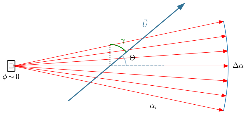
Arc scans are low and constant elevation radial-velocity measurements, performed along an arc of varying azimuth angles. A birds’-eye view illustration of the topology and fundamental parameters of an arc scan is shown in Figure 1.

The following parameters characterize the scan:

• $\varphi$ is the elevation of the scan, in this case near 0°.
• ${\alpha }_i$ is the azimuth of the line of sight (LOS) of each measurement i in the scan, where $i=1\dots N$.
• $\Delta \alpha$ is the span of the arc.
• $\mathbf{U}$ is the vector of the corresponding wind during the measurement.
• $\Theta$ is the difference between the wind direction of $\mathbf{U}$ and the Azimuth of the center of the arc scan.
• $\gamma$ is the wind direction, given in meteorological convention (0° refers to northern wind, increasing clockwise). Note that for an arc aligned to the north, $\gamma$ and $\Theta$ coincide.

Extraction of the two lateral wind components from the arc scans is based on the method of VAD scans [2]. For small elevation angles, the vertical wind component may be neglected. Under this assumption, the equation relating the radial-velocity measurements to the wind components is shown in Equation (1):

$$V_{ri}\left({\alpha }_i\right)=u·\sin \left({\alpha }_i\right)+v·\cos \left({\alpha }_i\right)$$

(1)

where $V_{ri}$ is the i-th radial wind measurement and ${\alpha }_i$ is the azimuth angle of LOS i. $\alpha$ is defined corresponding to meteorological convention, such that LOSs directed to the north, east, south, and west correspond to $\alpha =0°$, $\alpha =90°$, $\alpha =180°$, and $\alpha =270°$, respectively. u and v are the horizontal wind velocity components (westerly and northerly, respectively). Following Equation (1), the extraction equation is

$$\left(\begin{array}{c}u\\ v\end{array}\right)={\left(G^{T}G\right)}^{-1}{G}^T\left(\begin{array}{c}{V}_{r1}\\ ⋮\\ V_{rn}\end{array}\right)$$

(2)

where G is the $N\times 2$ matrix:

$$G=\left(\begin{array}{cc}\sin \left({\alpha }_1\right)& \cos \left({\alpha }_1\right)\\ ⋮& ⋮\\ \sin \left({\alpha }_n\right)& \cos \left({\alpha }_n\right)\end{array}\right).$$

(3)

In Equation (3), ordinary least squares is used instead of weighted least squares. We have found that, given the short time windows used here—motivated by operational constraints—the theoretical superiority of weighted least squares does not translate into superior retrieval performance. The generalized least squares formulation will be used in the following Section 3.2 only for uncertainty estimation.

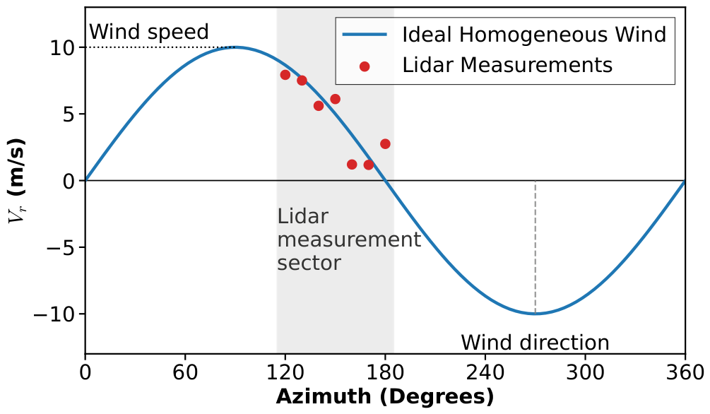
Figure 2 illustrates the unique challenge associated with arc scans, as opposed to full conical scans. The figure refers to an example in which the lateral wind direction is 270° (westerly wind). The blue harmonic curve corresponds to the radial-velocity ideally measured when the instrument LOS points to a given azimuth (x-axis). Extracting the curve’s amplitude and phase shift is directly related to the lateral wind speed and direction, respectively. Since the scan covers a limited azimuthal span $\Delta \alpha$, typically 30–60° (in the illustrated case between 120° and 180°), only part of the curve is “exposed” for measurement. The red dots illustrate measurements, where each dot is associated with a given azimuth. The deviation of the dots from the ideal curve represents the impact of spatial and temporal inhomogeneity. A fundamental source of uncertainty arises from estimating the amplitude and phase shift from noisy radial-velocity measurements confined to a relatively small $\Delta \alpha$.

3.2. Theoretical Framework for Extraction of Uncertainties

Following the generalized least squares formulation and Equation (2), the covariance matrix of the two lateral wind components is

$$\left(\begin{array}{cc}Var\left(u\right)& Cov(u,v)\\ Cov(u,v)& Var\left(v\right)\end{array}\right)={\left(G^{T}WG\right)}^{-1}$$

(4)

when $W\equiv {\Sigma }^{-1}$ is the weight matrix, which is the inverse of the $N\times N$ covariance matrix $\Sigma$ of the N radial-velocity measurements, defined as

$$\Sigma =\left(\begin{array}{cccc}\mathrm{Var}\left(V_{r1}\right)& \mathrm{Cov}\left(V_{r1}{V}_{r2}\right)& \dots & \mathrm{Cov}\left(V_{r1}{V}_{rn}\right)\\ \mathrm{Cov}\left(V_{r1}{V}_{r2}\right)& \mathrm{Var}\left(V_{r2}\right)& & ⋮\\ ⋮& & \ddots & \mathrm{Cov}\left(V_{r1}{V}_{rn}\right)\\ \dots & & & \mathrm{Var}\left(V_{rn}\right)\end{array}\right).$$

(5)

In rapid-scan operational configurations, a limited available scanning time per point of interest may yield fewer independent scans than the number of LOS orientations (N). Under these low-sample conditions, the empirical full covariance matrix $\Sigma$ becomes singular (rank-deficient), and its inversion to form the weight matrix W is challenging. Therefore, as a practical working regularization for real-time extraction, we neglect dependence between radial wind measurements with different orientations and define the diagonal weight matrix W as

$$W=\left(\begin{array}{cccc}1/{\sigma }_1^2& 0& \dots & 0\\ 0& 1/{\sigma }_2^2& \dots & 0\\ ⋮& ⋮& \ddots & ⋮\\ 0& 0& \dots & 1/{\sigma }_n^2\end{array}\right)$$

(6)

Here, ${\sigma }_i^2$ represents the temporal variance of individual LOS radial-velocities calculated over a 10 min window. Because atmospheric turbulence introduces strong temporal autocorrelation over 10 min windows, determining the exact effective sample size ($N_{eff}$) is non-trivial. Therefore, we utilize the raw temporal variance of the individual LOS radial-velocities as a conservative, upper-bound estimate of the retrieval uncertainty. The empirical validity and quantitative impact of this regularization are explicitly evaluated in Section 6.3.

Defining $M\equiv G^{T}WG$, we obtain

$$M=\left(\begin{array}{cc}\sum _i{\displaystyle \frac{{\sin }^2\left({\alpha }_i\right)}{{\sigma }_i^2}}& \sum _i{\displaystyle \frac{\cos \left({\alpha }_i\right)\sin \left({\alpha }_i\right)}{{\sigma }_i^2}}\\ \sum _i{\displaystyle \frac{\cos \left({\alpha }_i\right)\sin \left({\alpha }_i\right)}{{\sigma }_i^2}}& \sum _i{\displaystyle \frac{{\cos }^2\left({\alpha }_i\right)}{{\sigma }_i^2}}\end{array}\right)$$

(7)

Defining variables $a,b,c$ as

$$a\equiv \sum _i{\left({\displaystyle \frac{\sin {\alpha }_i}{{\sigma }_i}}\right)}^2;b\equiv \sum _i{\left({\displaystyle \frac{\cos {\alpha }_i}{{\sigma }_i}}\right)}^2;c\equiv \sum _i{\displaystyle \frac{\sin {\alpha }_i\cos {\alpha }_i}{{\sigma }_i^2}}$$

(8)

We write the covariance matrix of the lateral wind components as

$$M^{-1}={\displaystyle \frac{1}{ab-c^2}}\left(\begin{array}{cc}b& -c\\ -c& a\end{array}\right)$$

(9)

In the following, the Delta method is used to apply a transformation from variance in terms of Cartesian wind components to speed and direction representation. First-order error propagation states that

$$Var\left(f(u,v)\right)\approx {\left({\displaystyle \frac{\partial f}{\partial u}}\right)}^{2}Var\left(u\right)+{\left({\displaystyle \frac{\partial f}{\partial v}}\right)}^{2}Var\left(v\right)+2\left({\displaystyle \frac{\partial f}{\partial u}}{\displaystyle \frac{\partial f}{\partial v}}\right)Cov(u,v),$$

(10)

with f being the required parameter, either direction or speed. Meteorological horizontal speed U relates to the lateral Cartesian wind components as

$$U\equiv \sqrt{u^2+v^2}$$

(11)

Using the delta method, this yields

$$\begin{array}{cc}\hfill Var\left(U\right)\approx & {\left({\displaystyle \frac{\partial U}{\partial u}}\right)}^{2}Var\left(u\right)+{\left({\displaystyle \frac{\partial U}{\partial v}}\right)}^{2}Var\left(v\right)+2\left({\displaystyle \frac{\partial U}{\partial u}}{\displaystyle \frac{\partial U}{\partial v}}\right)Cov(u,v)\hfill \\ \hfill =& {\displaystyle \frac{1}{U^2}}\left(u^{2}Var\left(u\right)+v^{2}Var\left(v\right)+2uvCov(u,v)\right)\hfill \end{array}$$

(12)

Substituting from Equation (9) we obtain

$$Var\left(U\right)\approx {\displaystyle \frac{1}{U^2}}{\displaystyle \frac{u^{2}b+v^{2}a-2uvc}{ab-c^2}}$$

(13)

Similarly, we can calculate the variance of the direction. $\gamma$ is defined as the direction the wind is coming from in the meteorological convention, i.e., $\gamma =0°$ for wind coming from the north, $\gamma =90°$ for wind coming from the east, and so on. Therefore, it relates to the lateral wind components as

$$\gamma =\left(270-{\displaystyle \frac{180}{\pi }}\arctan 2(v,u)\right)(\mathrm{mod}360°)$$

(14)

And its derivatives are

$${\displaystyle \frac{\partial \gamma }{\partial u}}={\displaystyle \frac{180}{\pi }}{\displaystyle \frac{v}{u^2+v^2}}={\displaystyle \frac{180}{\pi }}{\displaystyle \frac{v}{U^2}},{\displaystyle \frac{\partial \gamma }{\partial v}}={\displaystyle \frac{180}{\pi }}{\displaystyle \frac{-u}{u^2+v^2}}=-{\displaystyle \frac{180}{\pi }}{\displaystyle \frac{u}{U^2}}$$

(15)

Substituting in Equation (10), we attain

$$\begin{array}{cc}\hfill Var\left(\gamma \right)\approx & {\left({\displaystyle \frac{\partial \gamma }{\partial u}}\right)}^{2}Var\left(u\right)+{\left({\displaystyle \frac{\partial \gamma }{\partial v}}\right)}^{2}Var\left(v\right)+2\left({\displaystyle \frac{\partial \gamma }{\partial u}}{\displaystyle \frac{\partial \gamma }{\partial v}}\right)Cov(u,v)\hfill \\ \hfill =& {\left({\displaystyle \frac{180}{\pi }}\right)}^2{\displaystyle \frac{1}{U^4}}\left(v^{2}Var\left(u\right)+u^{2}Var\left(v\right)-2uvCov(u,v)\right)\hfill \end{array}$$

(16)

This yields a direction variance:

$$Var\left(\gamma \right)\approx {\left({\displaystyle \frac{180}{\pi }}\right)}^2{\displaystyle \frac{1}{U^4}}{\displaystyle \frac{u^{2}a+v^{2}b+2uvc}{ab-c^2}}.$$

(17)

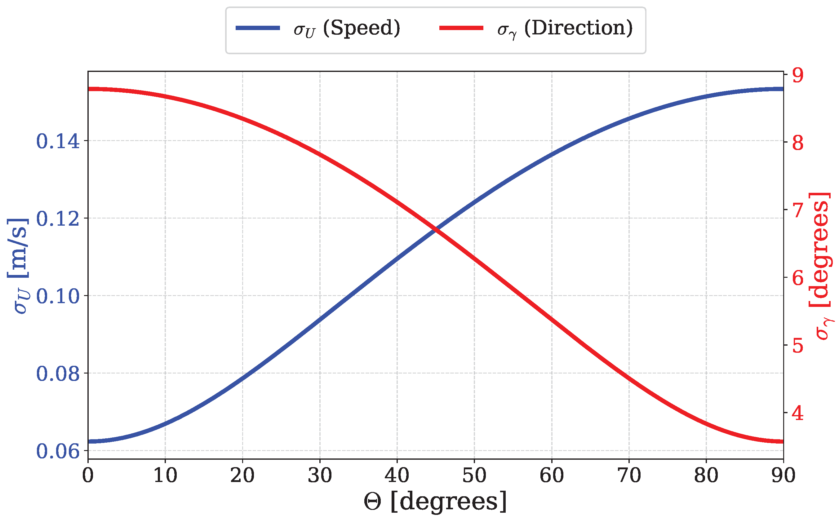
Standard deviations ${\sigma }_U$ and ${\sigma }_{\gamma }$, given by square root values of Equations (13) and (17), respectively, are plotted in Figure 3 for $U=1$, ${\sigma }_i=0.2$, $N=12$ and $\Delta \alpha =72°$, for varying $\Theta$. For Θ ≈ 0° (arc central axis directed parallel to the flow), velocity standard deviation is minimal, whereas direction standard deviation is relatively high. As $\Theta$ increases towards 90° (lidar view direction perpendicular to flow direction), the opposite occurs, as velocity standard deviation increases, and direction standard deviation decreases.

A note on ${\sigma }_{\gamma }$ should be made. Because wind direction is a circular variable, prediction intervals for wind direction should be calculated using a modulo operation: $P{I}_{\gamma }=(\gamma \pm {\sigma }_{\gamma })(\mathrm{mod}360°)$.

3.3. Impact of Arc Geometry on Uncertainty

In the following, we are interested in the impact of two key arc parameters, the arc span, $\Delta \alpha$, and the number of beams comprising the scan, N. Without loss of generality, we define an arc spanning the azimuth angles ${\alpha }_i=-\Delta \alpha /2+(i-1)\Delta \alpha /(N-1)$, with $i=1\dots N$. Assuming the same radial-velocity variance for all LOSs, i.e., ${\sigma }_i=\sigma$, and substituting in Equation (8), we now get

$$a={\displaystyle \frac{N}{2{\sigma }^2}}\left(1-\zeta \right);b={\displaystyle \frac{N}{2{\sigma }^2}}\left(1+\zeta \right);c=0$$

(18)

where

$$\zeta \equiv {\displaystyle \frac{1}{N}}{\displaystyle \frac{\sin (N\Delta \alpha /(N-1\left)\right)}{\sin (\Delta \alpha /(N-1\left)\right)}}$$

(19)

Substituting in Equations (13) and (17), we find

$$Var\left(U\right)={\displaystyle \frac{2{\sigma }^2}{N}}{\displaystyle \frac{{\sin }^2\left(\gamma \right)(1+\zeta )+{\cos }^2\left(\gamma \right)(1-\zeta )}{(1+\zeta )(1-\zeta )}}$$

(20)

$$Var\left(\gamma \right)={\left({\displaystyle \frac{180}{\pi }}\right)}^2{\displaystyle \frac{1}{U^2}}{\displaystyle \frac{2{\sigma }^2}{N}}{\displaystyle \frac{{\sin }^2\left(\gamma \right)(1-\zeta )+{\cos }^2\left(\gamma \right)(1+\zeta )}{(1+\zeta )(1-\zeta )}}$$

(21)

Since the defined arc directs at azimuth 0°, $\gamma$ is recognized as the arc-wind alignment angle $\Theta$. The wind speed variance rises with $\gamma$ monotonically between the limiting points:

$$Var\left(U\right){|}_{\Theta =\gamma =0°}={\displaystyle \frac{2{\sigma }^2}{N}}{\displaystyle \frac{1}{1+\zeta }};Var\left(U\right){|}_{\Theta =\gamma =90°}={\displaystyle \frac{2{\sigma }^2}{N}}{\displaystyle \frac{1}{1-\zeta }}$$

(22)

As expected, the opposite is true for the direction variance, which decreases monotonically between the points:

$$Var\left(\gamma \right){|}_{\Theta =\gamma =0°}={\left({\displaystyle \frac{180}{\pi }}\right)}^2{\displaystyle \frac{1}{U^2}}{\displaystyle \frac{2{\sigma }^2}{N}}{\displaystyle \frac{1}{1-\zeta }};Var\left(\gamma \right){|}_{\Theta =\gamma =90°}={\left({\displaystyle \frac{180}{\pi }}\right)}^2{\displaystyle \frac{1}{U^2}}{\displaystyle \frac{2{\sigma }^2}{N}}{\displaystyle \frac{1}{1+\zeta }}$$

(23)

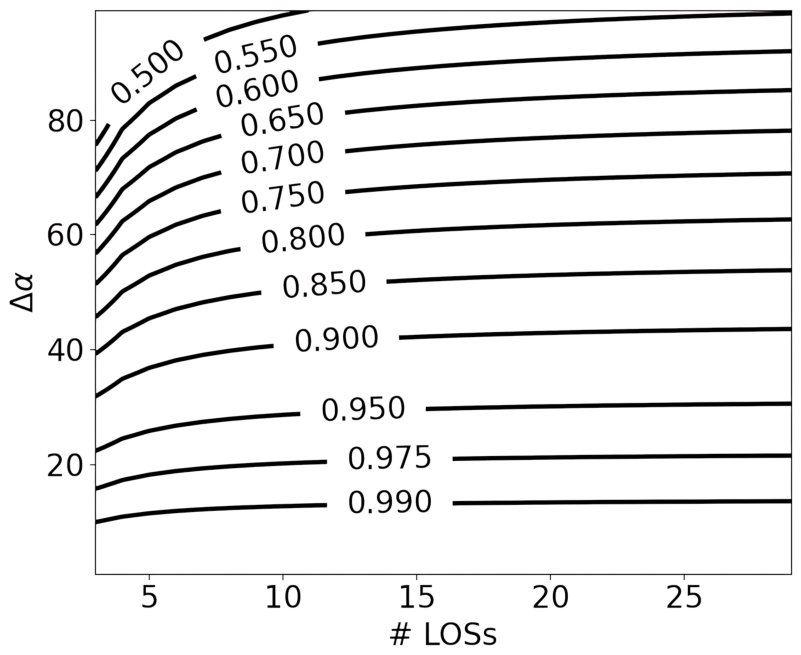
The dependence of the variance on N and $\Delta \alpha$ will be discussed with respect to these limiting points. The impact of $\Delta \alpha$ is entirely contained in $\zeta$. In Figure 4, $\zeta (N,\Delta \alpha )$ is plotted. For all N, $\zeta$ is monotonically decreasing with $\Delta \alpha$, where for $\Delta \alpha \to 0$, $\zeta \to 1$. This implies that for small arc spans, in the limiting cases of either $\Theta =0°$ or $\Theta =90°$, the direction variance, or the speed variance, respectively, diverges. At the same time, its counterpart variable reaches the minimal value ${\sigma }^2/N$. The N dependence is twofold. The main contribution to it comes from the prefactor ${\sigma }^2/N$, which is consistent with the central limit theorem. A weaker dependence is attributed to the impact of N on $\zeta$ (Figure 4), which is mostly significant for small values of N with large arc spans.

It should be noted that the design of the campaign described in the following included only one beam density, i.e., beams per arc span unit. This was done to have as large a number of scans as possible in the limited available time. Therefore, the dataset itself does not allow us to examine the impact of arc span and number of beams independently. The theoretical derivation presented in this subsection therefore remains subject to further validation.

4. Experimental Setup

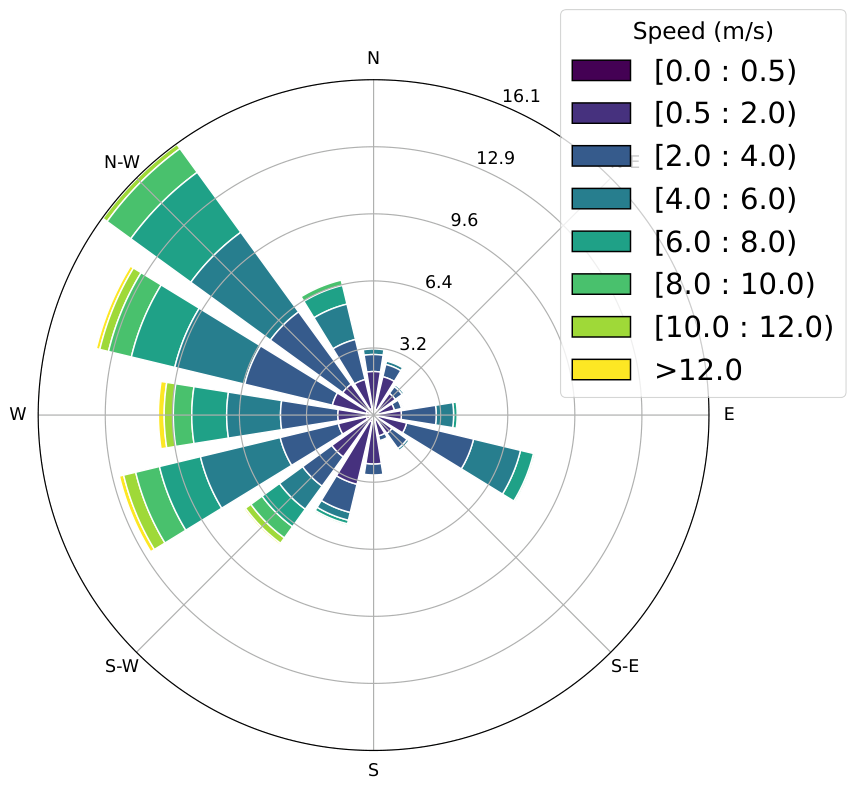
To evaluate the measurement method, an extensive field experiment was conducted. The campaign took place on the Sde-Boker campus of Ben-Gurion University in the south of Israel from January until May 2022. The wind regime at the site is presented in Figure 5 and is dominated by westerly winds.

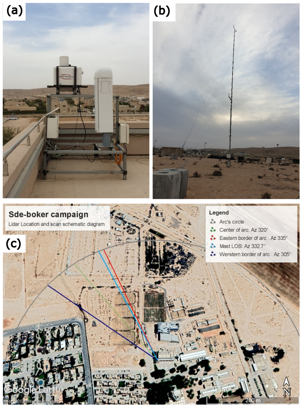
A StreamLine XR Doppler lidar (Halo Photonics, Malvern, UK; now Lumibird, Lannion, France) was positioned on the roof of the solar energy department building (Figure 6a) with a viewing angle to a meteorological mast located 375 m away (Figure 6b). An RM Young 81000 ultrasonic anemometer (R.M. Young Company, Traverse City, MI, USA) was mounted on the mast at 25 m above ground level. Another such anemometer was mounted at a height of 2 m and was used for meteorological classification. The StreamLine XR Doppler lidar provides full-sky measurement coverage, with outputs including range gate, Doppler wind speed, SNR+1, and attenuated backscatter. The lidar’s specifications are shown in

Table 1. StreamLine XR Doppler lidar specifications.

Specification	Value
Pulse sampling frequency	100 MHz
Laser wavelength	1550 nm
Laser repetition rate	10 kHz
Laser pulse length (FWHM)	310 ns
Output power (average)	400 mW
Average beam opening	60 µrad
Scanner elevation range	(−3)–+90°
Scanner angle resolution	0.2 mrad
Scanner angular speed	1020 mrad/s
Wind velocity range	±38 m/s
Wind velocity precision	0.04 m/s
Minimum range for measurements	30–40 m
Maximum range for measurements	6000–12,000 m
Range resolution	1.5 m
System dimensions in m (W × L × H)	0.6 m × 0.5 m × 0.4 m

.

The RM Young 81000 is a three-axis ultrasonic anemometer that measures the three-dimensional wind components and the sonic temperature; its specifications are shown in

Table 2. RM Young 81000 ultrasonic anemometer specifications.

Specification	Value
Wind speed range	0–40 m/s
Wind speed resolution	0.01 m/s
Wind speed accuracy	0–30 m/s: ±1% ± 0.05 m/s, 30–40 m/s: ±3%
Wind direction range	0–360°
Wind direction resolution	0.1°
Wind direction accuracy	1–30 m/s: ±2°, 30–40 m/s: ±5°
Sonic temperature	(−50)–50 °C
Sonic temperature accuracy	±2 °C
Temporal resolution	4–32 Hz (set to 32 Hz for this campaign)
Operating temperature	($-50$)–50 °C
Dimensions	56 cm high × 17 cm radius (3 support arms)
Weight	1.2 kg

.

The height difference between the lidar and the sonic anemometer dictates an elevation angle ϕ = 2.17°. The deviation of the elevation angle from the horizontal adds terms of the order of ${\sin }^2\left(\varphi \right){\sigma }_z^2$ to the radial-velocity variances, where ${\sigma }_z^2$ is the vertical velocity variance. Even for the extreme case of a highly convective boundary layer, the vertical velocity variance at a height of a few tens of meters above ground level is ${\sigma }_z^2\approx$ 1 m²s⁻² [14]. Therefore, a typical value for the radial-velocity variances attributed to vertical turbulent flow is $0.0014$. This value is much lower than the horizontal turbulent wind variance, which for convective boundary layers is usually around unity. Hence, applying the approximation of zero elevation angle for our observations is justified.

As shown in Figure 6c, the mast azimuth with respect to the lidar mounting point is 332.7°, and the scanning arc is defined between azimuth 305–335°. Given that the mast was located near the edge of the scanning arc and that some of the approach wind fetches crossed a residential area, part of the discrepancy observed in the comparison between mast data and lidar retrievals likely stems from the fact that mast data do not necessarily represent the entire arc. However, since the results presented below show good agreement between mast and lidar observations overall, it is reasonable to assume that this representativeness issue does not significantly affect our results.

Each scan consisted of about 11 LOSs. The scan mode that was used was continuous scanning mode (CSM). In this mode, the lidar’s motors do not stop between each measurement. This type of scan can produce a shorter scan cycle, but the azimuths of each LOS in the arc itself are less consistent, and the number of LOSs in each scan may vary by ∼1–3 from scan to scan. The scan recurrence time was 2.5 min, as other types of measurements were performed between successive arc scans. A single scan time span is about 13.5 s. The lidar operated with a 100 MHz sampling rate, yielding a 1.5 m range sampling interval. Radial wind speeds were processed using an 8-point (12 m) range-gate length. By applying a sliding overlap function, the system provides the output interval of 1.5 m. However, the true independent spatial resolution was limited by the laser’s 310 ns pulse duration, which corresponds to a physical scattering volume of approximately 46.5 m. Consequently, while the data output interval is 1.5 m, adjacent range gates are highly correlated.

A fundamental limitation of arc scans is the lack of simultaneous sampling across all azimuths. As mentioned, the lidar requires an average of 13.5 s to complete a single sweep. In the surface layer, typical Eulerian integral time scales for horizontal wind components range from approximately 10 to 40 s [14,15,16], depending on stability and wind speed. Because the 13.5 s scan time is of the same order of magnitude as the integral time scale of the energy-containing eddies, the assumption of a purely stationary wind vector across the sweep is frequently violated, particularly in convective conditions characterized by rapid turbulent evolution. While advanced spatio-temporal covariance models can theoretically address this (e.g., [13]), the least-squares framework naturally absorbs this scan-time evolution. Mid-scan turbulent shifts manifest as localized deviations from the idealized cosine projection, directly inflating the radial-velocity covariance. Consequently, the uncertainty generated by non-simultaneous sampling is implicitly quantified and bounded within the widened variance.

5. Methods of Evaluation

The theoretical framework derived above regards u and v as the spatially averaged wind components. Because deploying point wind instruments at multiple locations along the arc is impractical for a validation setup, and considering ergodicity together with the site characteristics discussed above, we assume in the following that the time-averaged wind observed at the sonic anemometer location is a good approximation of u and v. Wind speed and direction derived from 10 to min-averaged sonic measurements were compared with the corresponding values retrieved from arc scan lidar data, with the lidar retrievals likewise averaged over 10 min. To capture only the main trends, weak-wind cases (<0.5 m/s) were excluded. For this campaign, we used an SNR threshold of 0.025; this value was selected using an autocorrelation method [2,17,18], with a velocity stability threshold of 1 m/s.

As discussed above, because the lidar operated in continuous scanning mode, the exact azimuthal coordinates and the total number of line-of-sight (LOS) measurements varied between sweeps. However, the theoretical variance framework requires a uniform matrix of radial-velocities evaluated at fixed azimuths (N fixed angles, ${\alpha }_i$). To standardize the empirical data for covariance calculations, a spatial interpolation algorithm was applied to the individual scans. A uniform mathematical grid of N evenly spaced azimuths across the arc span was defined. The radial-velocities recorded during each irregular sweep were mapped onto this fixed grid using a Piecewise Cubic Hermite Interpolating Polynomial (PCHIP). PCHIP interpolation was utilized to preserve the monotonicity of the radial-velocity curve and to prevent unphysical overshoots between data points.

To examine the dependence of the uncertainty of the wind vector retrieval on $\Theta$, the data were divided into azimuthal sectors as shown in

Table 3. Measurement scenarios based on $\Theta$ sectors.

$\mathbf{\Theta }$	Measurement Scenario
0–10° and 170–180°	Parallel
10–20° and 160–170°	Near parallel
20–30° and 150–160°	Low obliquity
30–40° and 140–150°	Moderate obliquity
40–50° and 130–140°	Mid obliquity
50–60° and 120–130°	High obliquity
60–70° and 110–120°	Very high obliquity
70–80° and 100–110°	Near perpendicular
80–100°	Perpendicular

:

The validation of wind speed retrieval is based on the following parameters:

• Regression slope(a) and intercept (b) of the linear regression $v^L=a{v}^S+b$.
• Coefficient of determination ($R^2$), where 1 indicates perfect agreement:

  $$R^2={\left({\displaystyle \frac{{\sum }_i(v_i^S-\overline{v^S})(v_i^L-\overline{v^L})}{\sqrt{{\sum }_i{(v_i^S-\overline{v^S})}^2{\sum }_i{(v_i^L-\overline{v^L})}^2}}}\right)}^2.$$

  (24)
• Normalized root mean square error (NRMSE):

  $$NRMSE=\sqrt{{\displaystyle \frac{1}{n}}{\sum }_i{\left({\displaystyle \frac{v_i^S-v_i^L}{v_i^S}}\right)}^2},$$

  (25)

  where $v_i^S$ and $v_i^L$ are the velocities observed by sonic and lidar, respectively.

Unlike standard RMSE, which evaluates absolute differences and is often preferred in wind energy applications [19], the definition of NRMSE divides by $v_i^S$. This choice is dictated by our focus on hazardous-material dispersion modeling, where the concentration of contaminants is inversely proportional to wind speed ($C\propto 1/u$) [20]. By using a relative metric, we appropriately penalize lidar deviations during low-wind events, which correspond to the highest-risk stagnation scenarios. It should be noted that NRMSE is sensitive to the weak-wind threshold chosen. For a higher threshold of 1 m/s, NRMSE values decrease by a factor of 1.38.

For wind direction, a bias parameter is defined:

$$Bias={\displaystyle \frac{1}{N}}\sum _i{d}_i$$

(26)

where $d_i\equiv L_i-S_i$, with $L_i$ and $S_i$ the lidar and sonic wind-direction observations, respectively. The circular (periodic) nature of direction is addressed with the following correction:

$$d_i=\left\{\begin{array}{cc}{d}_i-360\hfill & \mathrm{if}{d}_i>180\hfill \\ d_i+360\hfill & \mathrm{if}{d}_i<-180\hfill \\ d_i\hfill & \mathrm{elsewhere}\hfill \end{array}\right.$$

(27)

To avoid fat tail effects, the interquartile range (IQR), the span between the 85th percentile and the 15th percentile of d, was chosen for quantification of error distribution width:

$$IQR=P_{85}\left(\left\{d\right\}\right)-P_{15}\left(\left\{d\right\}\right)$$

(28)

6. Results

6.1. Validation of Retrieved Speed and Direction

Table 4. Validation parameters for the agreement of lidar with mast observations for different wind-relative orientations. $R^2$ is the coefficient of efficiency (1 is perfect). NRMSE is the root mean square error of deviations, normalized by wind speed as observed by the sonic anemometer. a and b are linear fit coefficients for $v^L=a{v}^S+b$. Direction bias and the range between the 85th and the 15th quantile (IQR) of the wind direction deviations are also presented. n is the number of valid wind retrievals.

Θ Scenario	Speed Parameters					Direction Parameters
	${\mathit{R}}^{\mathbf{2}}$	NRMSE	$\mathit{a}$	$\mathit{b}$	$\mathit{n}$	Bias	IQR
Parallel	0.97	0.30	1.02	0.28	1933	−0.67°	24.31°
Near parallel	0.97	0.26	1.01	0.27	1702	1.71°	27.14°
Low obliquity	0.95	0.28	1.01	0.23	1290	3.09°	27.29°
Moderate obliquity	0.95	0.30	0.99	0.27	1065	2.78°	25.61°
Mid obliquity	0.96	0.25	1.00	0.22	948	−0.51°	24.70°
High obliquity	0.93	0.41	0.96	0.28	1138	1.58°	19.87°
Very high obliquity	0.95	0.26	1.02	0.13	1431	1.78°	15.14°
Near perpendicular	0.93	0.39	1.00	0.19	1150	−1.51°	17.54°
Perpendicular	0.90	0.32	0.95	0.22	974	−2.93°	17.26°

presents a comparison of lidar and sonic anemometer observations for each $\Theta$ segment using the above parameters. The following figures depict the comparison for speed (Figure 7) and direction (Figure 8), respectively.

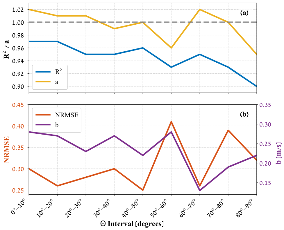
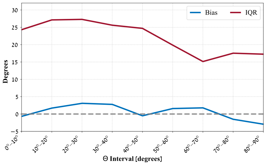
As shown in Figure 7, retrieved wind speed shows a moderate decline in $R^2$ with the increase in $\Theta$. For direction retrieval (Figure 8), while the bias does not show strong $\Theta$ dependence, the IQR declines with $\Theta$, reflecting relatively higher confidence in direction retrievals for Θ > ∼60°.

6.2. Analysis of Observed Speed and Direction Errors

In the following, we examine the dependence of wind speed and direction uncertainties on $\Theta$. This analysis should be interpreted in the context of the theoretical results presented in Section 3.2. The observational dataset covers an extensive period with a broad range of wind speeds, directions, and stability conditions, so the resulting mean uncertainties reflect the combined influence of multiple real-world factors. By contrast, the theoretical expressions were derived for a fixed wind speed and direction and are therefore not expected to reproduce the observed average uncertainties quantitatively when evaluated for a single configuration. Nevertheless, the measurements provide clear qualitative support for the theoretically predicted behavior, particularly the sensitivity to arc orientation. Moreover, we assess a direct practical consequence of the theoretical formulation by using it as an operational tool for estimating prediction intervals.

Additionally, we note that the theoretical sensitivity analysis with respect to arc width and number of beams, presented in Section 3.3, is not directly evaluated against the observations. This is because the measurement campaign was designed to prioritize robust estimation of overall retrieval uncertainty rather than a controlled assessment of sensitivity to scan-geometry parameters. The latter would require partitioning the scans into multiple arc configurations, thereby reducing the sample size within each subset and compromising statistical convergence. Dedicated future experiments will be required to address this aspect explicitly.

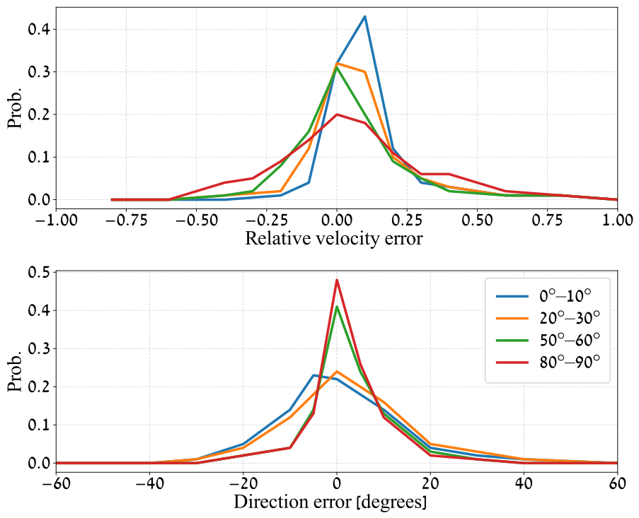
Figure 9 shows relative speed error probability distributions (defined as $2(v_i^L-v_i^S)/$$(v_i^L+v_i^S)$, upper panel) and wind direction error (Equation (26)). Distributions are shown for four selected $\Theta$ sectors: parallel, low obliquity, high obliquity, and perpendicular (curve colors blue, orange, green, and red, respectively). As $\Theta$ increases, the speed error distribution broadens, whereas the direction error distribution narrows. This manifests, observationally, the different impact of error propagation into speed and direction retrievals, as discussed in Section 3.1.

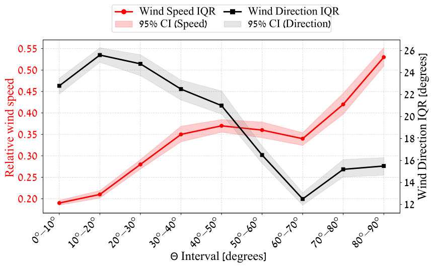
The same is manifested in Figure 10, presenting the IQR of the relative wind speed errors and wind direction errors as a function of $\Theta$ (with 95% bootstrap confidence intervals indicated by shaded regions). The IQR plotted in Figure 10 and the standard deviation plotted in Figure 3 are strictly different measures. Yet, qualitative resemblance to the theoretical results presented in Figure 3 can be observed.

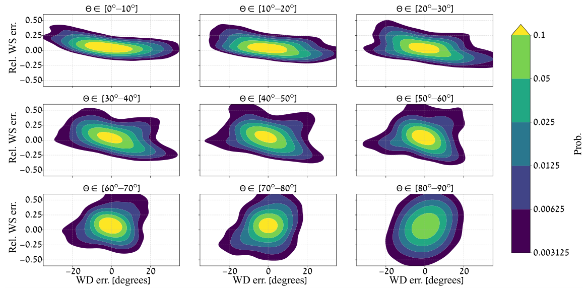
Figure 11 shows 2D histograms of the relative wind speed error (y-axis) and wind direction error (x-axis). Each subplot reflects the joint error probability distribution for a specific $\Theta$ range. Probability densities were evaluated using a Gaussian Kernel Density Estimate (KDE) with bandwidth selection governed by Scott’s rule. Again, in agreement with Figure 10, as $\Theta$ is altered from parallel to perpendicular, the range of wind speed errors grows larger, while the range of wind direction errors decreases. The 2D histograms reveal a dependence between direction and speed errors, which is most pronounced at intermediate values of $\Theta$. This reflects coupling between wind speed and direction errors. This can be understood through the covariance structure of the inversion. Since both u and v are estimated simultaneously from the same set of LOS velocities, their retrieval errors are not independent. At intermediate $\Theta$, off-diagonal terms of the covariance matrix (Equation (9)) are enhanced. Through error propagation, these nonzero covariance terms translate into a coupled uncertainty in speed and direction, such that overestimation of direction is typically associated with underestimation of speed, and vice versa.

It should be noted that the sample size n varies across the directional bins (Table 4), reflecting the prevailing wind climatology of the site (Figure 5). Despite the lower sample counts in certain oblique sectors, the consistency of the trends across adjacent bins indicates that the results are robust against sampling fluctuations.

6.3. Validation of the Diagonal Covariance Approximation

To evaluate the impact of utilizing only the diagonal elements of the covariance matrix—introduced as a practical regularization in Section 3.2—a comparative analysis was performed. Because for our measurements 10 min operational windows often yield rank-deficient matrices, the comparison utilized extended 40 min observation windows to ensure the invertibility of the full empirical covariance matrix. 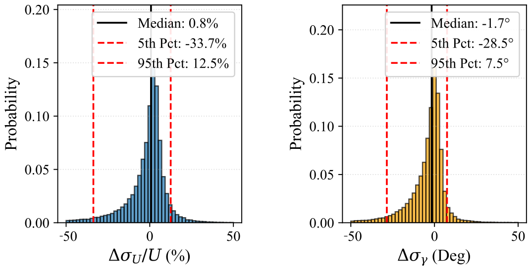Figure 12 presents the resulting differences between standard deviations calculated with the full covariance matrix and those calculated using the diagonal approximation ($\Delta \sigma ={\sigma }_{full}-{\sigma }_{diagonal}$).

For relative wind speed uncertainty, the median difference is merely 0.8%, with 5th and 95th percentiles at $-33.7$% and 12.5%, respectively. Similarly, the wind direction uncertainty exhibits a median difference of $-1.7$°, bounded by −28.5° and 7.5° at the 5th and 95th percentiles. These differences imply that the operational necessity leading to the neglect of off-diagonal covariance elements may have a substantial impact on the calculated uncertainty. For this reason, the origins of $\Delta \sigma$, in terms of spatial correlations and the distinct meteorological conditions that affect them, are studied in the following.

To quantify the spatial coherence of the wind field and assess the validity of the diagonal covariance approximation, a mean adjacent-beam correlation metric, R, was calculated for each averaging window. The calculation relies on the temporal variance of the radial-velocities. For a given averaging window containing Q scans, let $V_{r,i}\left(t\right)$ represent the radial-velocity measured at the i-th beam angle at time t. The temporal Pearson correlation coefficient, $r_{i,i+1}$, between an immediately adjacent beam pair (i and $i+1$) is defined as

$$r_{i,i+1}={\displaystyle \frac{{\sum }_{t=1}^Q(V_{r,i}\left(t\right)-{\overline{V}}_{r,i})(V_{r,i+1}\left(t\right)-{\overline{V}}_{r,i+1})}{\sqrt{{\sum }_{t=1}^Q{(V_{r,i}\left(t\right)-{\overline{V}}_{r,i})}^2{\sum }_{t=1}^Q{(V_{r,i+1}\left(t\right)-{\overline{V}}_{r,i+1})}^2}}},$$

(29)

where ${\overline{V}}_{r,i}$ is the temporal mean of the radial-velocity for the i-th beam over the window. To represent the overall spatial correlation across the entire scanning sector for that window, the scalar metric R was computed as the arithmetic mean of the correlation coefficients of all $N-1$ adjacent beam pairs:

$$R={\displaystyle \frac{1}{N-1}}{\displaystyle \sum _{i=1}^{N-1}}{r}_{i,i+1}.$$

(30)

This formulation isolates the macroscopic, coherent turbulent structures spanning multiple lines of sight, which are responsible for driving the off-diagonal terms in the full covariance matrix.

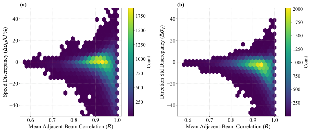
Figure 13 presents the dependency of $\Delta {\sigma }_U/U$ (Figure 13a) and $\Delta {\sigma }_{\gamma }$ (Figure 13b) on R. For both cases, high discrepancy is associated with high adjacent beam correlation.

To study the effect of different static stability conditions on the adjacent beam correlation R and hence on $\Delta \sigma$, we used the difference $\Delta T$ between the sonic temperature at height 2 m and at height 25 m. Stability classes were derived according to [21]. It is noted that sonic temperatures are virtual temperatures, while the scheme [21] is calibrated for dry-bulb temperature gradients. However, the exceptionally dry conditions at the site render the vertical specific humidity gradient negligible. 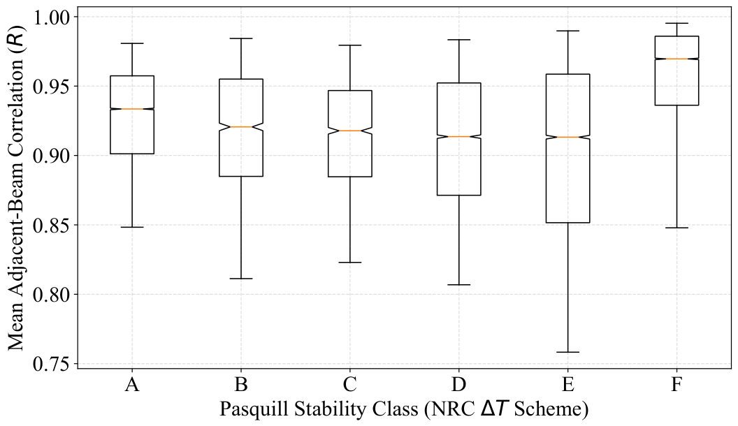Static stability influence on R is displayed in Figure 14. High R values are associated with either unstable convective conditions or with the extremely stable state F. The possible causes of high R therefore originate in two distinct boundary layer flow characteristics. In convective boundary layers, thermals are formed. These are large coherent structures that contribute to spatial correlation. For highly stable regimes, vertical turbulent fluctuations are damped, while horizontal 2D coherent structures emerge, which contribute to horizontal spatial correlation [14].

In the following, the validity of our approximation will also be examined in terms of the impact on prediction intervals (PIs).

6.4. Prediction Bounds Based on Variance Estimates

In the following, PIs for speed and direction, based on the formulation for variance estimation, will be examined against statistics of measurement errors. The covariance matrix $\Sigma$ was obtained by calculating 60 min radial-velocity statistics. The standard deviation of speed and direction was calculated by applying Equations (13) and (17). In addition, to study the relative impact of using only the diagonal elements of the covariance matrix $\Sigma$, the calculation was repeated with the full $\Sigma$, using $M={\left(G^T{\Sigma }^{-1}G\right)}^{-1}$ instead of Equation (7).

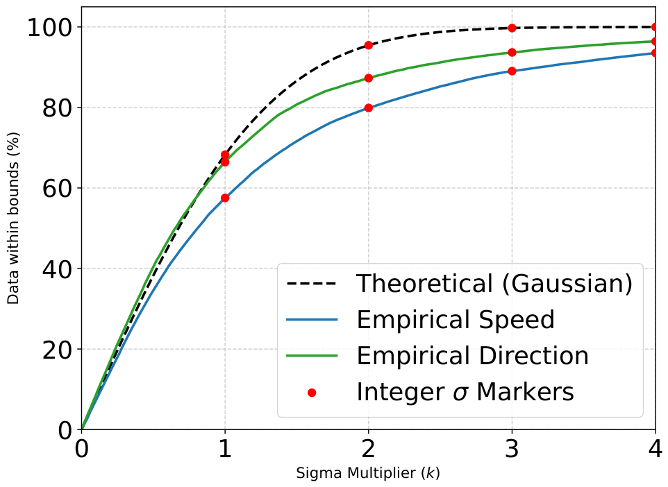
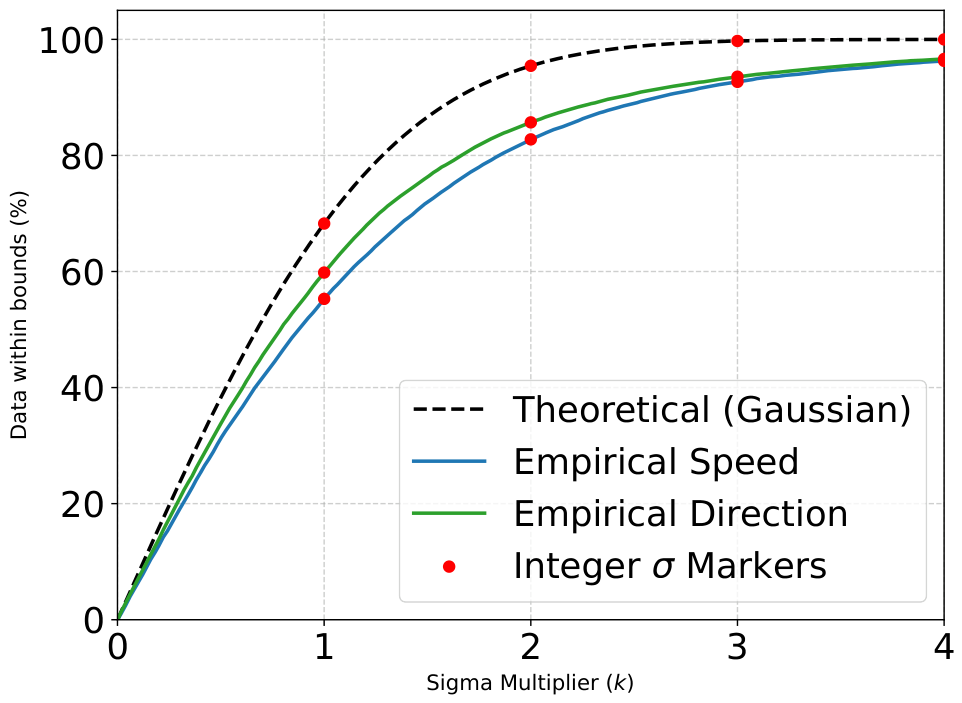
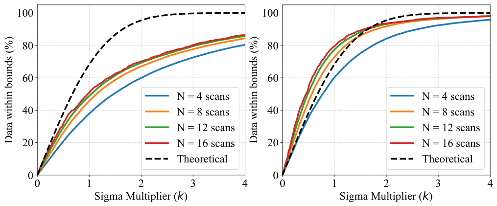
Figure 15 and Figure 16 show the empirical coverage probability (ECP) for speed and direction, for full $\Sigma$ and diagonal-only $\Sigma$ cases, respectively. In these figures, ECP is given as the percent of mast observations found within $k\sqrt{Var}$ from the retrieved speed or direction, as a function of k, where $Var$ is the variance of wind speed or direction. Coverage for the standard normal distribution is given for reference. ECP hardly changes with the relative angle, and this analysis is therefore not shown.

For both full and diagonal $\Sigma$ cases, and for both speed and direction, ECP for $k=1$ is lower but close to the normal distribution reference. For higher values of k, ECP stays considerably lower than the normal distribution reference.

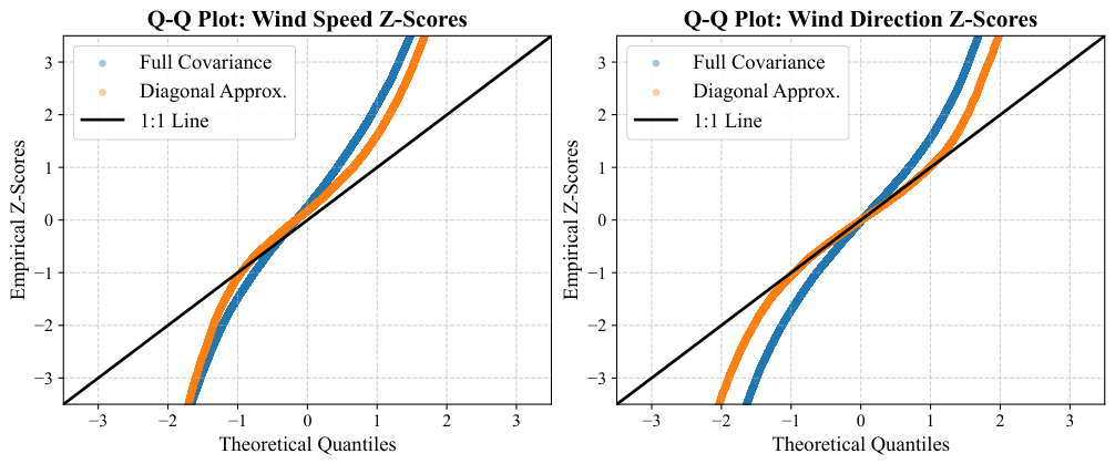
A similar impression can be viewed in Figure 17, presenting quantile–quantile (Q-Q) plots for speed and direction, for the diagonal-only covariance matrix and the full covariance matrix derivations. The plots test the quantile statistics of the observed deviations against those of the normal distribution and include a 1:1 reference line. The combined Q–Q analysis shows that both the full-covariance and diagonal-only uncertainty formulations reproduce the central portion of the normalized error distributions reasonably well. However, both exhibit systematic outward curvature relative to the 1:1 reference line for $\left|z\right|>1$, revealing heavier-than-Gaussian tails. This is consistent with the reduced empirical coverage at larger prediction-interval multipliers observed in Figure 15 and Figure 16.

This subsection is concluded with a conditional analysis of the robustness of evaluated uncertainty under distinct atmospheric conditions. To achieve this, the impact of turbulence intensity (TI, defined as $Std\left(U\right)/U$) and wind speed (WS) on the coverage probability was studied. Both TI and WS were evaluated based on mast observations, and variance estimation in the following was done using the diagonal elements of $\Sigma$. 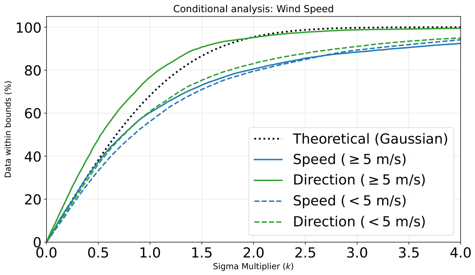Figure 18 shows ECP plots of direction and speed, where the dataset is partitioned into strong WS (>5 m/s) and weak WS (<5 m/s). 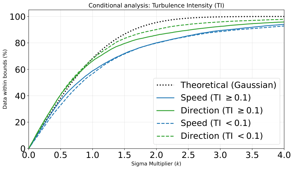Likewise, Figure 19 presents the same analysis, where the data is split into strong (>0.1) and weak (<0.1) TI. It is important to emphasize that the various atmospheric parameters that can impact uncertainty estimation are heavily entangled; therefore, any impact of WS and TI may indirectly relate to other parameters that cannot be isolated in field measurements.

As Figure 18 and Figure 19 show, wind speed uncertainty coverage is hardly affected by WS or TI. However, the analysis reflects a dependence of directional uncertainty coverage on WS and also mildly on TI. For strong winds, the direction standard deviation shows over-coverage up to $k=2$, whereas for weak winds, the direction ECP is lower than the normal-distribution reference. This might be attributed to high spatial homogeneity associated with strong winds. Regarding the impact of TI, estimated direction uncertainty coverage is slightly closer to the normal distribution reference for weaker turbulence.

6.5. Impact of Averaging Window Duration on Statistical Convergence and Coverage Reliability

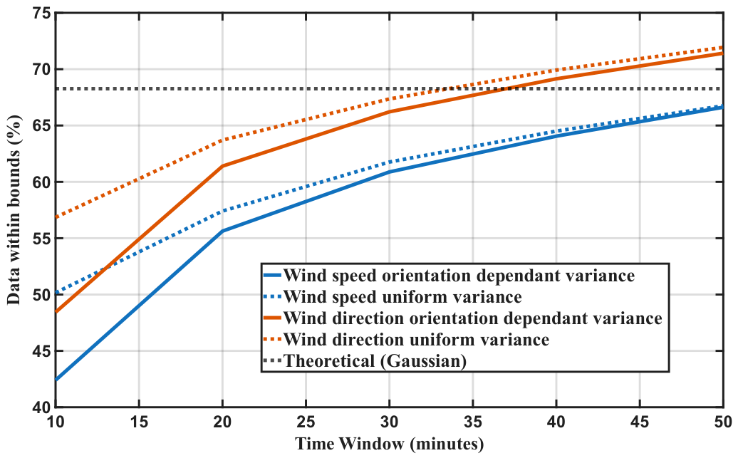
To evaluate how limited sample sizes impact the coverage of the prediction bounds, we analyzed the $1\sigma$ ECP across increasing observation-window durations (10 to 50 min). Expanding the window artificially increases the scan count, simulating the transition from a constrained, low-sample operational mode to a fully converged statistical state. Additionally, we tested two variance regularizations to address low-sample noise.

• Orientation-dependent variance: calculating discrete variances (${\sigma }_i^2$) strictly for each independent line-of-sight beam.
• Uniform variance: averaging variances across the entire arc to yield a spatially uniform scalar for the diagonal weight matrix W.

Figure 20 illustrates the model’s sensitivity to statistical convergence. In the highly constrained 10 min scenario, the standard orientation-dependent formulation is vulnerable to variance noise, resulting in under-dispersive bounds (∼42% coverage for speed, ∼$48\%$ for direction). However, as the scan count increases (represented by the 40–50 min windows), the empirical coverage converges directly toward the theoretical Gaussian expectation ($68.3\%$), reaching ∼$66\%$ and ∼$71\%$ for speed and direction, respectively.

It should be noted that the theoretical coverage assumes a standard Gaussian distribution. However, because the variance defining the uncertainty bounds for each 10 min window is estimated from a very small sample size ($N\le 4$), the statistically rigorous expectation follows a Student’s t-distribution. The ‘heavier tails’ of the t-distribution mean that expected coverage for small samples is naturally lower than Gaussian targets (e.g., 58% vs. 68.3% at $1\sigma$). Therefore, evaluating these specific bounds against a Gaussian reference inherently makes the ECP appear somewhat under-dispersive.

Importantly for real-time applications, Figure 20 demonstrates that variance regularization mitigates the penalty of low scan counts. By applying the uniform variance formulation to the data-starved 10 min windows, the $1\sigma$ coverage improves to ∼$50\%$ for speed and ∼$57\%$ for direction, filtering out beam-specific sampling noise.

Practical operational evolution of empirical coverage probabilities as observation windows are extended over time inherently couples statistical sample-size growth with physical temporal filtering. To decouple these effects and isolate the pure statistical convergence of the variance estimator, a stationary-segment subsampling analysis was conducted. By isolating 40 min windows characterized by stationary flow conditions (wind direction standard deviation ≤10° and wind speed coefficient of variation ≤$12\%$), the physical time scale and atmospheric turbulence spectrum were held relatively constant. Scan datasets within these blocks were then randomly subsampled at discrete densities of $N\in \{4,8,12,16\}$. As shown in Figure 21, the ECPs exhibit systematic convergence toward the theoretical Gaussian expectation as sample size increases. However, the improvement saturates between $N=12$ and $N=16$ scans, indicating that further increasing scan density yields diminishing returns for variance estimation.

7. Conclusions

This study presents a closed-form analytical framework for estimating PIs of wind speed and direction retrieved from Doppler lidar arc scans. The derivation, based on generalized least squares and first-order error propagation, links the uncertainties of retrieved wind vectors directly to observable and controllable factors: the standard deviation of line-of-sight (LOS) radial-velocity measurements, arc scan geometry, and the relative orientation between the mean wind and the arc center.

The derived formulation reveals a geometric tradeoff between optimal minimization of wind direction and wind speed retrieval uncertainty. While the first is minimized for large relative angles ($\Theta$) between the center of the arc and the average wind direction, the latter is minimized for small relative angles. This result is valuable for campaign planning and siting.

This tradeoff is qualitatively supported by a campaign including lidar retrievals and sonic anemometer measurements. The observed deviations between retrieved wind and sonic anemometer data qualitatively exhibit the predicted dependency on arc orientation. Specifically, small relative orientation ($\Theta$ angle) reduces the uncertainty of wind speed retrievals, while large relative orientation reduces the uncertainty of wind direction retrievals.

Importantly, the framework accommodates heterogeneous LOS variances, reflecting real measurement variability. By deriving the prediction intervals solely from the diagonal variance terms, the model provides a practical mathematical regularization. This enables stable, real-time inversion in rapid-update operational scenarios where the low number of scans renders the empirical full covariance matrix singular while maintaining a geometry-aware formulation adaptable to various deployment scenarios.

Validation against independent sonic anemometer data included studying the impact of the suggested regularization and the source of discrepancies between uncertainty assessments done with and without applying it. In addition, coverage percentage performance for different time windows and sample sizes was examined. Specifically, the following results were obtained:

• Direction and speed uncertainties are sensitive to the regularization of the covariance matrix $\Sigma$. Individual uncertainty calculations may yield considerably different results when performed with or without the approximation of retaining only diagonal elements. However, when tested over relatively long time windows, applying the proposed approximation does not significantly change the ECPs compared to ECPs attained using the complete covariance matrix.
• The largest discrepancies between uncertainties evaluated using the approximation and using the full covariance matrices are found particularly under very unstable or very stable conditions. These conditions are characterized by high correlation between radial-velocities measured at adjacent beams.
• Direction prediction bounds are conservative (over-covering) under strong-wind conditions but somewhat under-covering with weak winds, plausibly reflecting greater spatial wind homogeneity at higher wind speeds.
• Statistical convergence of the variance of the radial wind velocity is important for proper estimation of prediction bounds. This is reflected by testing coverage probabilities using different time-range windows and by block-sampling analysis. Statistical convergence for short time windows can be partially mediated by applying uniform variance across arc beams.

The current field campaign confirms the model’s qualitative dependence on wind-arc alignment over flat terrain. However, the single-site observational dataset does not fully demonstrate general applicability. Future work must systematically evaluate the framework’s sensitivity across different scan geometries (e.g., varying arc spans and beam numbers), more complex terrain types, and diverse atmospheric stability regimes. Expanding validation across various conditions, alongside incorporating correlated LOS variances, will be essential to fully establishing the robustness and generality of the framework.

Overall, this study serves as an important step towards the uncertainty-aware use of arc scans for operational environmental applications requiring fast, multi-location wind field assessment.

References

- Browning, K.A.; Wexler, R. The determination of kinematic properties of a wind field using Doppler radar. J. Appl. Meteorol. Climatol. 1968, 7, 105–113. [Google Scholar] [CrossRef] [Scilit]
- Tzadok, T.; Ronen, A.; Rostkier-Edelstein, D.; Agassi, E.; Avisar, D.; Berkovic, S.; Manor, A. Profiling the Planetary Boundary Layer Wind with a StreamLine XR Doppler lidar: Comparison to In-Situ Observations and WRF Model Simulations. Remote Sens. 2022, 14, 4264. [Google Scholar] [CrossRef] [Scilit]
- Newsom, R.K.; Brewer, W.A.; Wilczak, J.M.; Wolfe, D.E.; Oncley, S.P.; Lundquist, J.K. Validating precision estimates in horizontal wind measurements from a Doppler lidar. Atmos. Meas. Tech. 2017, 10, 1229–1240. [Google Scholar] [CrossRef] [Scilit]
- Frehlich, R. Errors for space-based Doppler lidar wind measurements: Definition, performance, and verification. J. Atmos. Ocean. Technol. 2001, 18, 2045–2053. [Google Scholar] [CrossRef] [Scilit]
- Sathe, A.; Mann, J. A review of turbulence measurements using ground-based wind lidars. Atmos. Meas. Tech. 2013, 6, 3147–3167. [Google Scholar] [CrossRef] [Scilit]
- Wang, H.; Barthelmie, R.J.; Clifton, A.; Pryor, S.C. Wind Measurements from Arc Scans with Doppler Wind lidar. J. Atmos. Ocean. Technol. 2015, 32, 2024–2040. [Google Scholar] [CrossRef] [Scilit]
- Banta, R.K. Stable-boundary-layer regimes from the perspective of the low-level jet. Acta Geophys. 2008, 56, 58–87. [Google Scholar] [CrossRef] [Scilit]
- Simon, E.I.; Courtney, M.S. A Comparison of Sector-Scan and Dual Doppler Wind Measurements at Høvsøre Test Station—One Lidar or Two? DTU Wind Energy Report E-0112; DTU Wind Energy: Roskilde, Denmark, 2016; Available online: https://backend.orbit.dtu.dk/ws/portalfiles/portal/125285452/RUNE_D1.2_ellsim_final.pdf (accessed on 12 August 2026).
- Doubrawa, P.; Barthelmie, R.J.; Wang, H.; Pryor, S.C.; Churchfield, M.J. Wind turbine wake characterization from temporally disjunct 3-D measurements. Remote Sens. 2016, 8, 939. [Google Scholar] [CrossRef] [Scilit]
- Choukulkar, A.; Brewer, W.A.; Sandberg, S.P.; Weickmann, A.; Bowen, T.A.; Turner, D.D.; Lundquist, J.K. Evaluation of single and multiple Doppler lidar techniques to measure complex flow during the XPIA field campaign. Atmos. Meas. Tech. 2017, 10, 1471–1483. [Google Scholar] [CrossRef] [Scilit]
- Aitken, M.L.; Banta, R.M.; Pichugina, Y.L.; Lundquist, J.K. Quantifying Wind Turbine Wake Characteristics from Scanning Remote Sensor Data. J. Atmos. Ocean. Technol. 2014, 31, 1529–1539. [Google Scholar] [CrossRef] [Scilit]
- Pauscher, L.; Vasiljevic, N.; Callies, D.; Lea, G.; Mann, J.; Klaas, T.; Hieronimus, J.; Gottschall, J.; Schwesig, A.; Kühn, M.; et al. An Inter-Comparison Study of Multi- and DBS lidar Measurements in Complex Terrain. Remote Sens. 2016, 8, 782. [Google Scholar] [CrossRef] [Scilit]
- Wang, H.; Barthelmie, R.J.; Pryor, S.C.; Brown, G. Lidar arc scan uncertainty reduction through scanning geometry optimization. Atmos. Meas. Tech. 2016, 9, 1653–1669. [Google Scholar] [CrossRef] [Scilit]
- Stull, R.B. An Introduction to Boundary Layer Meteorology; Springer: Dordrecht, The Netherlands, 2012. [Google Scholar]
- Kaimal, J.C.; Finnigan, J.J. Atmospheric Boundary Layer Flows: Their Structure and Measurement; Oxford University Press: New York, NY, USA, 1994. [Google Scholar]
- Panofsky, H.A.; Dutton, J.A. Atmospheric Turbulence: Models and Methods for Engineering Applications; John Wiley & Sons: New York, NY, USA, 1984. [Google Scholar]
- Liu, Z.; Barlow, J.F.; Chan, P.-W.; Fung, J.C.H.; Li, Y.; Ren, C.; Mak, H.W.L.; Ng, E. A Review of Progress and Applications of Pulsed Doppler Wind LiDARs. Remote Sens. 2019, 11, 2522. [Google Scholar] [CrossRef] [Scilit]
- Newsom, R.K.; Krishnamurthy, R. Doppler Lidar (DL) Instrument Handbook; DOE/SC-ARM/TR-101; DOE Office of Science Atmospheric Radiation Measurement (ARM) User Facility: Oak Ridge, TN, USA, 2020.
- Brower, M. Wind Resource Assessment: A Practical Guide to Developing a Wind Project; John Wiley & Sons: Hoboken, NJ, USA, 2012. [Google Scholar]
- Arya, S.P. Air Pollution Meteorology and Dispersion; Oxford University Press: New York, NY, USA, 1999. [Google Scholar]
- U.S. Nuclear Regulatory Commission. Meteorological Monitoring Programs for Nuclear Power Plants. In Regulatory Guide 1.23; Revision 1; U.S. Nuclear Regulatory Commission: Rockville, MD, USA, 2007. [Google Scholar]
Figure 1.
Birds’-eye illustration of low elevation arc scan, with parameters describing the configuration. is the elevation angle. is the azimuth of the i-th beam (), and is the arc span. , and are the mean wind direction, the relative angle between the wind and the arc main axis, and the horizontal wind vector, respectively.
Figure 2.
Radial-velocity
as a function of LOS azimuth for an idealized homogeneous wind field with direction 270°-westerly wind (blue curve). Red dots show simulated lidar measurements within the sampled arc sector (gray shading, 120–180° in this example), illustrating how only a limited portion of the full harmonic curve is observed. The scatter of the dots around the ideal curve represents the combined effect of spatial/temporal wind inhomogeneity, which is the principal source of retrieval uncertainty addressed in
Section 3.2.
Figure 3.
Theoretically predicted standard deviations of retrieved wind speed (
, blue, left axis) and wind direction (
, red, right axis) as a function of the arc–wind alignment angle
, computed from Equations (
13) and (
17) for
m/s,
beams, and
. Speed uncertainty is minimized, and direction uncertainty maximized when the arc is aligned with the wind (Θ ≈ 0°); the opposite holds near perpendicular alignment (Θ ≈ 90°).
Figure 4.
Contour plot of the geometric factor
(Equation (
19)) as a function of the number of beams per scan (
N) and the arc span (
, degrees).
governs the sensitivity of the speed and direction variances to arc–wind alignment (Equations (
20)–(
23)):
for narrow arcs, causing divergence of either the speed or direction variance at the limiting alignment angles. Conversely, as
increases,
declines, and so is the sensitivity of uncertainty to limiting values of
.
is sensitive to
N only for low
N values.
Figure 5.
Wind rose at the mast location for the full campaign period (January–May 2022), colored by wind speed bin. Radial ticks present the percent of occurrence. South-southwesterly to northwesterly winds dominate the record.
Figure 6.
Meteorological campaign set up in Sde-Boker. (a) StreamLine XR Doppler lidar on the roof of the solar energy department. (b) Meteorological mast sonic anemometer 25 m above ground. (c) Google Earth imagery © 2022 Google, showing the lidar location, the arc scan sector (red and purple lines), and the sonic anemometer mast line-of-sight (light-blue line).
Figure 7.
Wind speed validation parameters as a function of