A Practical Framework for Surface Water Extraction from GF1/GF6 Wide-Field-View Imagery

Highlights

What are the main findings?

• A practical surface water extraction framework was developed for GF1/GF6 widefield view imagery by integrating multispectral features, topographic information, and water indices.
• The proposed framework achieved accurate and operationally applicable water mapping over large-scale scenes, with improved boundary delineation and reliable area estimation.

What are the implications of the main findings?

• The framework provides a transferable solution for large-scale surface water monitoring using Chinese high-resolution satellite imagery.
• The results support operational applications such as water-resource monitoring, flood assessment, and remote-sensing-based environmental management.

Abstract

Gaofen-1/Gaofen-6 (GF1/GF6) wide-field-view (WFV) imagery provides repeated wide-area observations for regional surface-water monitoring, but its use is complicated by fragmented water patterns, vegetation–water mixtures, terrain and cloud shadows, and cross-scene radiometric variability. This study presents a seven-channel nested U-Net (UNet++) framework with a residual logit refinement branch (RLRB) for binary surface-water extraction. The input combines Blue, Green, Red, near-infrared, normalized difference water index, normalized difference vegetation index, and digital-elevation-model-derived slope channels. Five complete GF1/GF6 scenes were locked before dataset partitioning, and an 8192 m exclusion buffer was used to exclude spatially overlapping or adjacent non-test tiles from model development, thereby reducing the risk of spatial leakage. The resulting quantitative test set contained 2783 valid 512 by 512 pixel tiles derived from the five scenes withheld at scene level. The UNet++ model with RLRB and edge-consistency supervision achieved an mIoU of 0.941, Water IoU of 0.889, and Water F1 of 0.941. A controlled $2\times 2$ experiment separated the effects of residual refinement and edge-consistency supervision, while feature, loss-component, random-seed, rule-based-baseline, and complete-scene analyses further characterized the framework. Complete-scene sliding-window inference required approximately 3.7 min per scene on a single NVIDIA GeForce RTX 5060 Laptop GPU, demonstrating the feasibility of georeferenced water-mask generation under the specified computational setting.

1. Introduction

Surface water bodies, including lakes, reservoirs, rivers, ponds, wetlands, and temporary inundation areas, are fundamental components of terrestrial hydrological and ecological systems. Accurate and timely information on their spatial distribution supports water resource assessment, flood emergency response, ecological conservation, irrigation management, and river-lake supervision. Satellite remote sensing has become a principal data source for large-area surface-water monitoring because it provides repeated observations over broad spatial extents with lower field-survey requirements than extensive ground-based mapping. The global surface water record demonstrates the value of satellite archives for quantifying long-term water dynamics [1], and complementary monitoring studies further show their usefulness for riverine and flood-related changes [2]. Recent reviews indicate that optical water extraction has gradually evolved from single-index rules toward multi-source, multi-temporal, and learning-based approaches [3,4,5].

Optical spectral indices have long been used for open-water delineation. The normalized difference water index (NDWI) proposed by McFeeters [6] enhances water by contrasting the Green and near-infrared (NIR) bands, while the modified NDWI (MNDWI) improves the separability of water from built-up land by replacing the NIR band with a short-wave infrared band [7]. Other thresholding and index-selection methods, including the automated water extraction index (AWEI) and histogram-based thresholding, remain useful for rapid candidate extraction and label initialization [8,9]. However, GF1/GF6 WFV scenes can contain backgrounds that violate the assumptions of fixed or weakly adaptive thresholding.Mountain shadows, cloud shadows, dark roofs, asphalt roads, and moist bare soil can exhibit water-like spectral responses, whereas elongated channels, fragmented ponds, and vegetation–water mixtures may be spectrally discontinuous. Consequently, a threshold selected for one scene or region can produce substantial commission and omission errors elsewhere.

GF1 and GF6 are important components of the Chinese Gaofen Earth observation constellation. The GF1 WFV system provides broad coverage with a combined swath of approximately 800 km, making it useful for regional-scale monitoring, although wide-view observations also introduce cross-camera and angular radiometric variability [10]. Cloud and cloud-shadow detection in GF1/GF6 WFV imagery is also challenging because the spectral configuration used in many operational workflows contains mainly visible and NIR information [11,12]. High-resolution Gaofen interpretation benchmarks have further shown that segmentation from domestic high-resolution imagery requires methods that are robust to large scene size, diverse land-cover backgrounds, and annotation noise [13]. These characteristics are directly relevant to water extraction: the wide swath is advantageous for regional mapping, but radiometric inconsistency, limited spectral discrimination, and complex shadows reduce the robustness of purely rule-based water masks.

Deep-learning-based semantic segmentation provides a way to learn contextual and multi-scale representations from labelled remote-sensing data. Fully convolutional networks enable end-to-end dense prediction [14]; U-Net combines high-level semantic information with low-level spatial detail through encoder–decoder skip connections [15]; DeepLabV3+ strengthens contextual modelling through atrous multi-scale representation and decoder refinement [16]; and UNet++ introduces nested dense skip pathways to reduce the semantic gap between encoder and decoder features [17]. Current water-extraction research can therefore be organized around multi-scale representation, contextual modelling, boundary-aware learning, and cross-scene generalization rather than around individual architectures alone. Dice-style overlap losses address foreground imbalance [18], Tversky loss permits asymmetric control of false positives and false negatives [19], and explicit edge supervision provides complementary boundary information [20,21].

In water extraction, early learning-based studies demonstrated the feasibility of mapping surface water from multispectral satellite imagery [22,23], and high-resolution urban-water research showed that convolutional models can handle more complex object boundaries and background mixtures [24]. For the Gaofen family, MWEN and LMSWENet are representative examples of multi-scale convolutional water extraction from GF-1 and GF-1D imagery [25,26]. Subsequent studies refined this direction through high-resolution UAV water analysis [27], richer convolutional feature design [28], multi-scale residual learning [29], and feature-aggregation modules [30]. Domain-adaptation studies have examined cross-scene robustness [31,32], while augmentation-based Sentinel-2 experiments provide another data-centric route [33]. More recent networks have introduced transformer-assisted representations through WaterFormer [34] and enhanced U-Net formulations for water segmentation [35]. Other recent optical water-extraction studies continue to improve the balance between accuracy and model practicality [36,37]. Nevertheless, practical GF1/GF6 WFV mapping still requires careful adaptation to semi-automatic label construction, multi-source input design, thin-water continuity, shadow suppression, and full-scene inference.

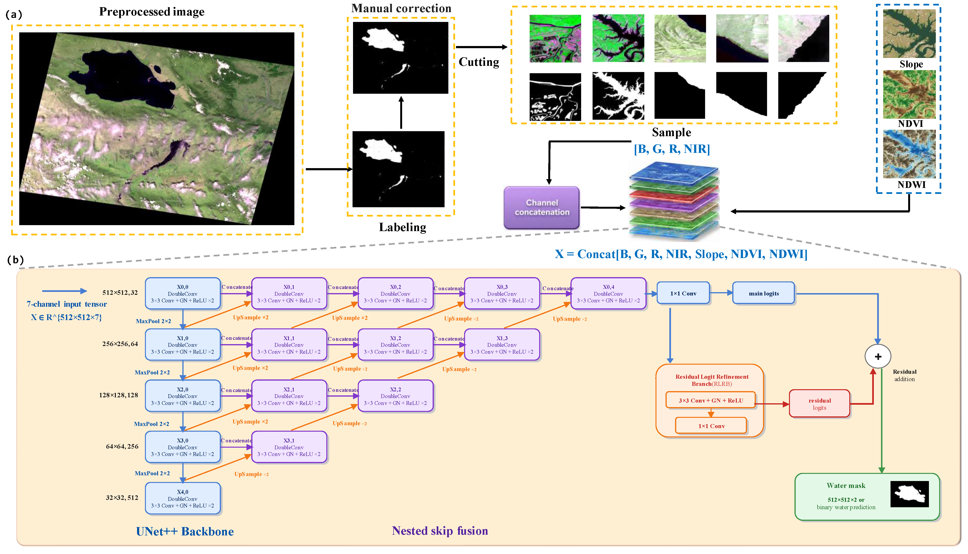
The proposed processing chain and model structure are summarized in Figure 1, linking image preprocessing, candidate-mask generation, manual correction, seven-channel feature construction, UNet++ nested decoding, and residual-logit refinement.

This study addresses these needs by developing a seven-channel UNet++ framework with an RLRB for GF1/GF6 surface-water mapping. Rule-based thresholding accelerates candidate-mask generation, after which evident commission errors, omissions, and local boundary offsets are manually corrected. The model integrates Blue, Green, Red, NIR, digital-elevation-model (DEM) slope, NDWI, and normalized difference vegetation index (NDVI) channels and applies a deliberately low-capacity residual correction to the final logits. The main contributions are as follows:

• A seven-channel input configuration integrates four multispectral bands, two spectral indices, and DEM-derived slope; controlled feature ablations quantify the contributions of the optical, index, and topographic components.
• A lightweight RLRB is attached to the final UNet++ decoder representation. A $2\times 2$ factorial experiment separates its residual-refinement effect from that of the independently controlled edge-consistency loss.
• A scene-level spatial evaluation protocol locks five complete scenes before partitioning and excludes spatially adjacent candidates through an 8192 m buffer, reducing the risk of train–test leakage.
• A complete GF1/GF6 workflow is evaluated from rule-based initialization and QGIS-assisted label correction to seven-channel training, georeferenced full-scene inference, NoData masking, and raster/vector output.

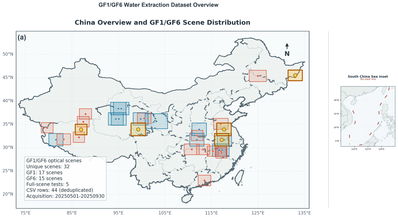
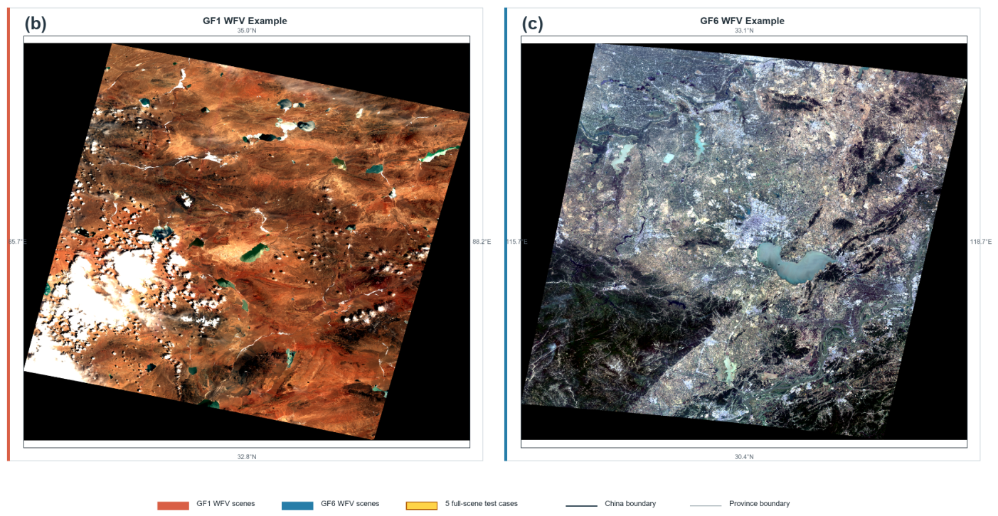
Figure 2 summarizes the dataset distribution and representative preprocessed WFV scene examples. The upper panel shows the nationwide distribution of the 32 GF1/GF6 optical scenes and the five withheld test scenes, while the lower panels illustrate typical GF1 and GF6 WFV image geometry, NoData regions, and diverse land–water background conditions after preprocessing.

2. Related Work

2.1. Spectral-Index-Based Surface Water Extraction

Spectral-index methods remain widely used for optical water extraction because they are transparent, computationally efficient, and easy to deploy. NDWI uses the contrast between the Green and NIR bands to enhance open water [6], while MNDWI improves water/background separation in many urban scenes by introducing SWIR information [7]. AWEI was proposed to reduce shadow-related confusion, and adaptive thresholding remains a common component in semi-automatic mask generation [8,9]. Multi-index and rule-based water-mapping methods have also been widely applied to optical satellite data [3,4]. In the present GF1/GF6 workflow, NDWI is valuable because Blue, Green, Red, and NIR bands are consistently available. Nevertheless, index thresholds remain sensitive to scene-dependent illumination, land-cover background, atmospheric conditions, and sensor differences. The present study therefore treats the rule-based output as a transparent initialization baseline and evaluates it against the manually corrected reference masks.

2.2. Deep Semantic Segmentation for Remote-Sensing Water Mapping

Deep convolutional segmentation networks learn nonlinear combinations of spectral and spatial features and can represent objects with complex shape and context. FCN introduced dense end-to-end prediction [14], U-Net strengthened encoder–decoder segmentation with skip connections [15], DeepLabV3+ used atrous spatial pyramid pooling and an improved decoder [16], and UNet++ redesigned skip pathways to reduce the encoder–decoder semantic gap [17]. Remote-sensing reviews and benchmark studies indicate that deep segmentation has become a dominant approach for high-resolution land-cover interpretation [38,39]. Transferability and annotation quality remain major challenges, especially for large domestic high-resolution scenes [13,40]. For water extraction, DeepWaterMap and Landsat CNN water extraction are representative early deep-learning studies [22,23], while high-resolution urban water mapping demonstrates the need to handle detailed boundaries and mixed non-water backgrounds [24]. Gaofen-oriented networks such as MWEN and LMSWENet further support the feasibility of learning-based water extraction from Chinese high-resolution optical imagery [25,26]. Recent work has then explored residual feature enhancement [28,29]. Domain adaptation and data augmentation have been studied to improve cross-scene robustness [31,32], with augmentation-based Sentinel-2 experiments providing a related data-centric perspective [33]. Multi-scale feature aggregation [30], transformer-assisted design [34], and enhanced U-Net variants [35] further show how recent networks strengthen contextual water representation. These studies support the feasibility of learning-based water extraction, while the present work focuses specifically on GF1/GF6 WFV seven-channel spectral-topographic fusion and full-scene operational inference.

2.3. Edge-Aware Supervision and Residual Refinement

Water mapping is sensitive to shoreline continuity and boundary displacement. Deep edge-detection and boundary-aware segmentation studies explicitly supervise edge responses rather than treating them only as implicit products of region classification [20,21]. Residual refinement, by contrast, can modify the final class logits without constituting an independently supervised edge head. This distinction is important here: the proposed RLRB receives only the final UNet++ decoder feature, contains no image-gradient or label-boundary input, and produces a two-class residual-logit correction. Edge supervision is introduced separately through an edge-consistency loss calculated from the final segmentation probability. The architecture is therefore described as residual logit refinement rather than as an inherently edge-aware branch, and the two mechanisms are controlled independently in the factorial experiment.

2.4. Multi-Source Feature Fusion in Optical Remote Sensing

Multi-source feature fusion is widely used in remote-sensing segmentation because different input channels describe complementary physical and spatial properties. Multimodal urban remote-sensing studies have shown that combining spectral, elevation, and contextual information can improve feature discrimination [41,42]. Transferability studies also suggest that richer input representations can help reduce the dependence of a model on a single scene distribution [40]. In water extraction, multi-scale residual modules and feature-aggregation networks illustrate the value of combining local texture, spectral response, and broader semantic context [29,30]. Transformer-assisted and enhanced U-Net studies further show that contextual representations are useful when water boundaries are fragmented or mixed with complex backgrounds [34,35]. For surface water mapping, multispectral bands, vegetation-sensitive indices, water indices, and topographic variables are often complementary: NDWI enhances water separability [6], AWEI targets shadow-related confusion [8], and reviews consistently emphasize the need to handle scene-dependent background variability [3,4]. The proposed seven-channel design follows this line of feature fusion but tailors it to the spectral availability and operational constraints of GF1/GF6 WFV imagery.

3. Study Area and Data

3.1. GF1/GF6 WFV Imagery and Spatial Coverage

The GF1/GF6 WFV data were obtained through the data-service workflow of the China Centre for Resources Satellite Data and Application. The collection contains 32 scenes acquired in two short 2025 windows, 1–10 May and 15–30 September, comprising 17 GF1 and 15 GF6 scenes; the 10 GF1 L2F scenes are included within this total. Scene selection jointly considered coverage of both sensors, eastern, central, western, and different-latitude regions of China, plains, mountains, plateau terrain, varied water morphologies, shadow-prone backgrounds, valid coverage, data completeness, and annotation feasibility. The scenes therefore represent two warm-season acquisition windows rather than continuous temporal coverage; this design limits snow-, ice-, and low-sun-angle variation but does not establish seasonal or interannual generalization.

Some source products overlap geographically because they are separate scene files acquired by different cameras, orbits, or times. They were retained to preserve wide-swath continuity and distinct observation conditions, but intersecting footprints were handled explicitly during partitioning so that spatially overlapping or adjacent tiles from non-test scenes could not enter the development pool. Five complete scenes were locked before dataset partitioning and were excluded from training and validation. The quantitative test set comprised 2783 valid 512 by 512 pixel tiles derived from those locked scenes, while the complete scenes were additionally used for full-scene inference.

3.2. Image Preprocessing

The modelling workflow used georeferenced GF1/GF6 GeoTIFF surface-reflectance scenes supplied by the institutional preprocessing chain. Before delivery, all scenes underwent the same standardized sequence of radiometric calibration, 6S-based atmospheric correction to surface reflectance, orthorectification, and geometric fine correction using Tianditu imagery as the spatial reference. The delivered surface-reflectance products were used directly in the modelling workflow, without any additional conversion from digital numbers or radiance. For each complete scene and optical band, valid pixels were clipped to the 2nd–98th percentile interval and linearly normalized to reduce numerical-range differences among input scenes.

No explicit cloud or cloud-shadow mask and no cross-sensor spectral harmonization, such as spectral-response-function correction, histogram matching, or sensor-to-sensor regression, were applied. Consequently, residual GF1/GF6 spectral-response differences may remain, and unmasked cloud or shadow pixels may influence the scene-level percentile distributions used for normalization and may reduce cross-scene comparability.

An optical pixel was considered valid only when all four optical bands were finite, differed from the GeoTIFF NoData value (falling back to 65,535 when missing), and were not simultaneously zero. NDWI and NDVI inherited this optical mask. Slope pixels were additionally required to be finite and different from the slope-raster NoData value. Invalid positions were set to zero after channel construction and were excluded from the reported output masks.

3.3. Tile Preparation, Split, and Quality Control

The initial tiling process produced 18,978 candidates. A tile was retained when its optically valid fraction, $f_{\mathrm{valid}}$, satisfied

$$f_{\mathrm{valid}}={\displaystyle \frac{1}{{512}^2}}{\displaystyle \sum _{i=1}^{{512}^2}}\mathbb{I}\left[i\mathrm{is}\mathrm{optically}\mathrm{valid}\right]\ge 0.98.$$

(1)

DEM slope, NDWI, and NDVI did not determine whether a candidate passed this tile-level threshold. After validity screening and the spatially independent partitioning procedure described below, 18,461 valid tiles were retained in the final dataset.

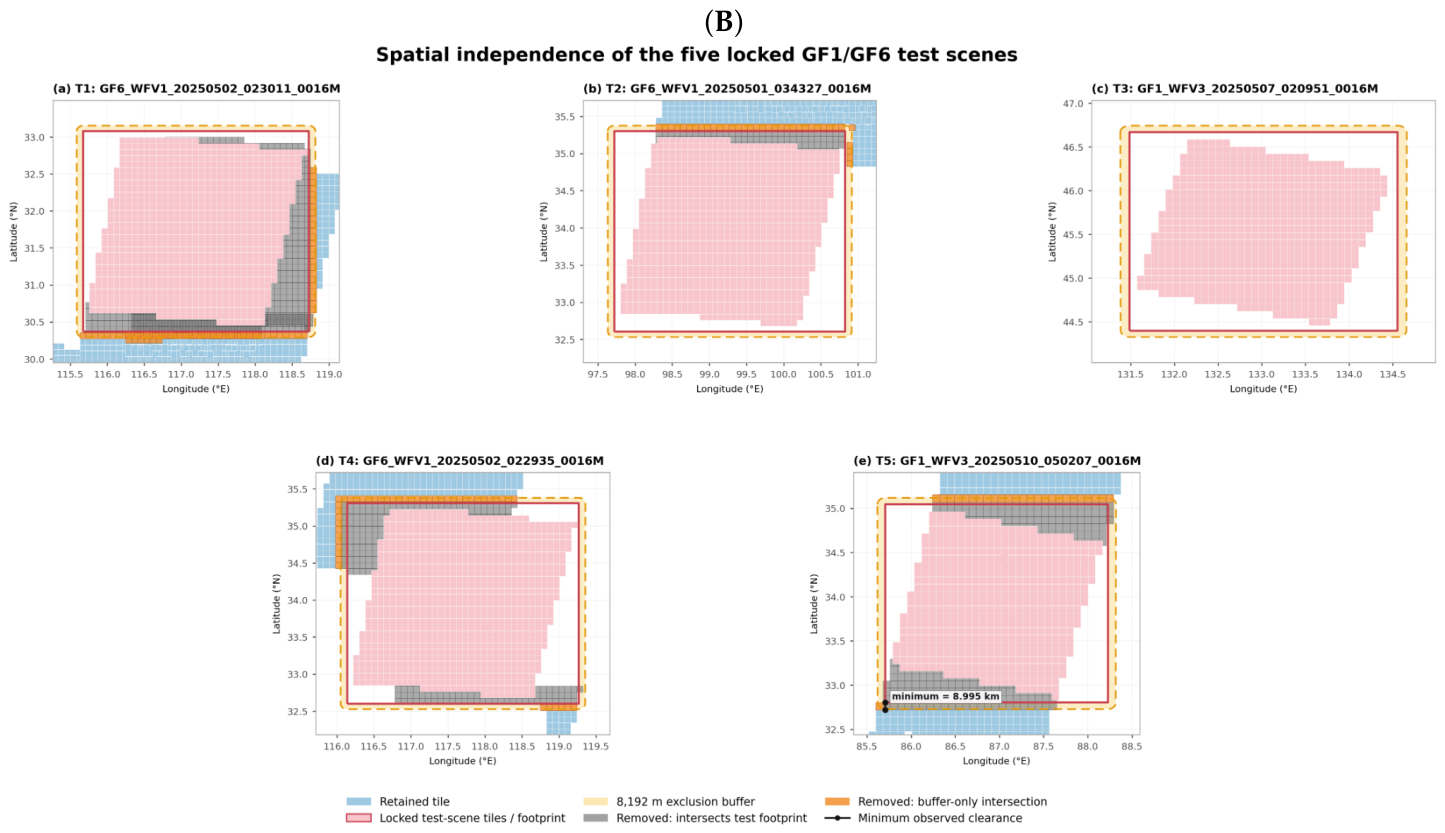
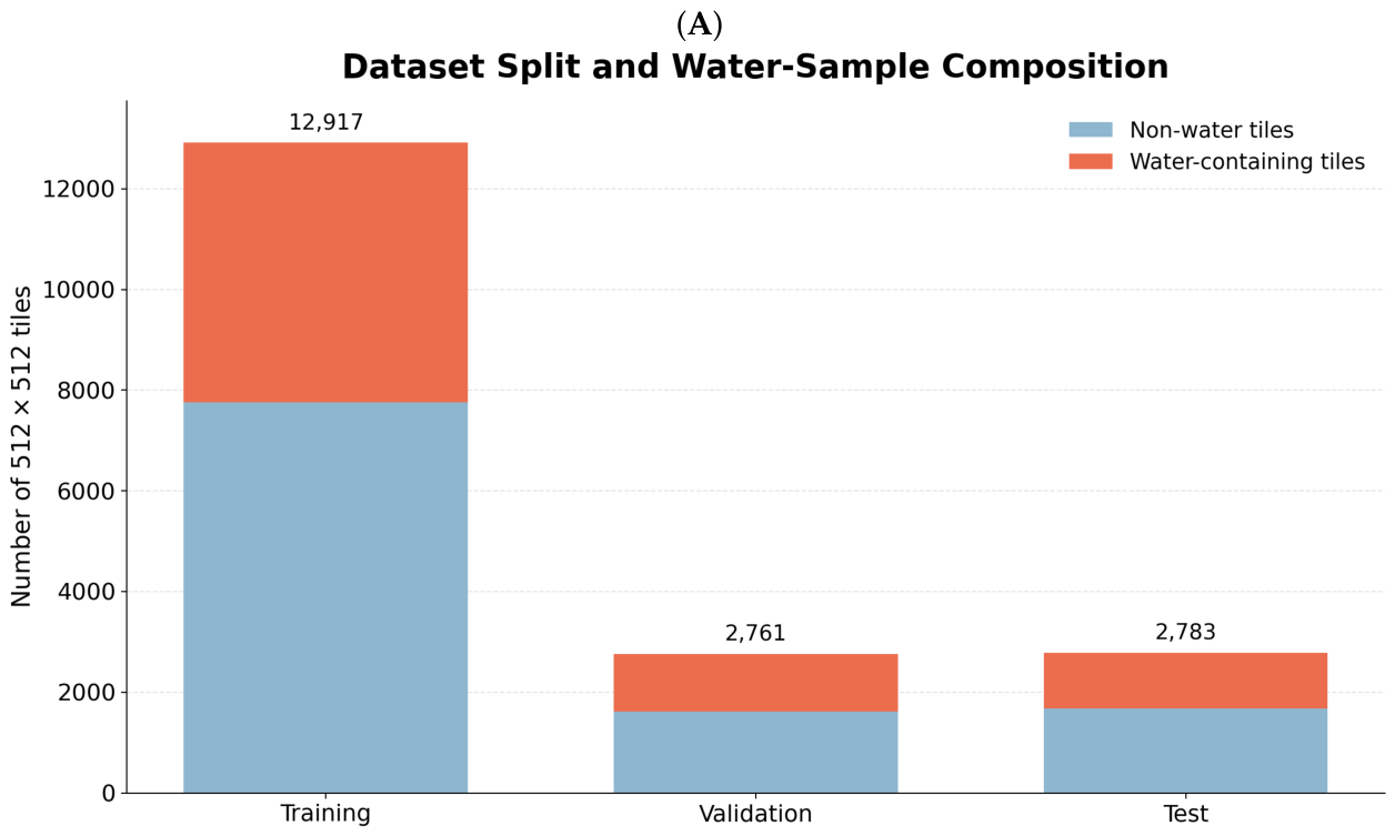
Spatial independence was enforced during the original dataset partitioning. Five complete GF1/GF6 scenes were first locked as independent test scenes, and no tile derived from them entered training or validation. An 8192 m outward buffer, corresponding to the nominal ground width of one $512\times 512$ input tile, was constructed around each locked footprint. Candidate tiles from all other scenes were excluded if they intersected either a test footprint or its buffer. Only the remaining non-test candidates were randomly divided into training and validation sets. The resulting fixed partition contains 12,917 training tiles, 2761 validation tiles, and 2783 test tiles (

Table 1. Statistics of valid tiles in the training, validation, and test sets.

Split	Valid Tiles	Water-Containing Tiles	Non-Water Tiles	Water Ratio (%)	Non-Water Ratio (%)
Training	12,917	5162	7755	39.96	60.04
Validation	2761	1140	1621	41.29	58.71
Test	2783	1106	1677	39.74	60.26
Total	18,461	7408	11,053	40.13	59.87

). The final retained tile counts contributed by each of the 32 source scenes are reported in Supplementary Table S1. A subsequent spatial audit confirmed the separation encoded by this original procedure and measured a minimum observed clearance of $8.995$ km (Figure 3); no dataset reconstruction or repartitioning was performed for this analysis.

3.4. Semi-Automatic Label Construction and Manual Correction

For each complete scene, NDWI was computed as $(G-N)/(G+N+{10}^{-6})$, clipped to $[-1,1]$, and summarized with a 2048-bin histogram. A separate Otsu threshold $T_{\mathrm{Otsu}}$ was estimated for every scene using the maximum between-class variance criterion [9]. The initial spectral candidate was

$$M_0=(\mathrm{NDWI}>T_{\mathrm{Otsu}})\wedge (N<1200),$$

(2)

where 1200 refers to the stored numerical scale of the supplied surface-reflectance GeoTIFF. This fixed value was retained as a conservative empirical setting for candidate-mask initialization rather than as a universally optimal threshold. In an exploratory check on one representative GF6 scene, increasing the threshold from 1200 to 1400, 1600, and 1800 increased the retained candidate-water pixel count by 17.2 percent, 40.9 percent, and 75.6 percent, respectively, and increased the number of vector components by 29.3 percent, 75.7 percent, and 133.2 percent, indicating progressively more extensive and fragmented candidate regions. Because this check involved only one scene and was not evaluated directly against the manually corrected reference masks, it is not interpreted as a formal multi-scene threshold optimization. An 8-connected GDAL sieve filter was then applied to raster components smaller than 128 pixels, after which invalid slope pixels and pixels with slope greater than ${10}^{\circ }$ were excluded:

$$M={Sieve}_{128,8}\left(M_0\right)\wedge (0^{\circ }\le S\le {10}^{\circ }).$$

(3)

NDVI, cloud or cloud-shadow quality layers, and additional opening or closing operations were not used in this rule. Without explicit cloud and cloud-shadow masking, shadow pixels with low NIR responses can satisfy the fixed threshold and increase commission errors, while contaminated pixels can also affect the scene-level percentile normalization applied to the model inputs. The uncorrected output is retained as the rule-based initialization baseline in Section 6.

Candidate masks were subsequently inspected and corrected in QGIS. Evident shadow-related commission errors were removed, and conspicuous omissions and local boundary offsets were edited before rasterization back to the original grid. Because the corrected references originated from these candidates, comparison with the uncorrected masks quantifies the limitations of the automatic initialization and the benefit of the correction-and-learning workflow; it is not presented as a comparison with an unrelated external method.

3.5. DEM-Derived Slope

Terrain slope was derived in Google Earth Engine from the Copernicus DEM GLO-30 2024_1 digital surface model (COPERNICUS/DEM/GLO30_2024_1) [43]. Slope in degrees was calculated using ee.Terrain.slope(), which evaluates the local gradient from four-connected neighbours [44]. The product was exported as 32-bit floating-point GeoTIFF tiles at a nominal 30 m resolution in EPSG:4326, mosaicked, and resampled by bilinear interpolation to each GF1/GF6 image grid. DEM-derived slope has been used in related optical water-mapping workflows to suppress dark responses associated with steep terrain and terrain shadows [45,46]. In the present network it is supplied as an input feature rather than used as a hard prediction mask.

3.6. Full-Scene Inference Cases

Five complete scenes were withheld from model development: T1, GF6_WFV1_20250502_023011_0016M; T2, GF6_WFV1_20250501_034327_0016M; T3, GF1_WFV3_20250507_020951_0016M; T4, GF6_WFV1_20250502_022935_0016M; and T5, GF1_WFV3_20250510_050207_0016M. The 2783-tile quantitative test set was derived from these scenes, and complete-scene outputs were additionally evaluated to reveal scene-level differences that can be obscured by a single pooled tile-level result. Because all five locked test scenes were acquired in May, this split evaluates scene-level spatial transfer rather than temporal or seasonal generalization.

4. Methodology

4.1. Overall Workflow

The framework integrates preprocessing, semi-automatic label construction, seven-channel feature generation, UNet++ with RLRB training, tile-level evaluation, and complete-scene sliding-window inference (Figure 1). The rule-based method is used both to initialize manual annotation and as an evaluated baseline.

4.2. Seven-Channel Spectral-Topographic Feature Construction

Let B, G, R, and N denote the Blue, Green, Red, and NIR bands of a GF1/GF6 WFV tile. The input tensor is constructed as

$$\mathbf{X}=\left[B,G,R,N,S,\mathrm{NDVI},\mathrm{NDWI}\right],$$

(4)

where S is the DEM-derived slope aligned to the GF1/GF6 image grid. NDWI and NDVI are computed as

$$\mathrm{NDWI}={\displaystyle \frac{G-N}{G+N+ϵ}},$$

(5)

$$\mathrm{NDVI}={\displaystyle \frac{N-R}{N+R+ϵ}},$$

(6)

where $ϵ={10}^{-6}$.

The four optical bands retain spectral information that may be compressed in a single index; NDWI enhances water–land contrast; NDVI supplies vegetation-sensitive information; and slope supplies topographic context. Each optical band is independently normalized with the scene-level 2nd and 98th valid-pixel percentiles. NDWI and NDVI are clipped to $[-1,1]$ before channel construction, and slope is normalized separately. This numerical normalization is applied consistently to both sensors but is not equivalent to spectral-response-function harmonization.

4.3. UNet++ Backbone

UNet++ is selected as the main segmentation backbone because its nested skip pathways gradually combine low-level spatial detail with high-level semantic information [15,17]. Given the input tensor $\mathbf{X}$, the backbone produces the final decoder feature $\mathbf{F}$ and the baseline two-class logits ${\mathbf{Z}}_0$:

$$\mathbf{F}=f_{\mathrm{UNet}++}\left(\mathbf{X}\right),{\mathbf{Z}}_0=f_{1\times 1}\left(\mathbf{F}\right),$$

(7)

where $f_{1\times 1}$ denotes a $1\times 1$ convolution that maps decoder features to two-class logits.

4.4. Residual Logit Refinement Branch

Code-level inspection confirmed that the refinement branch receives only the final decoder feature $\mathbf{F}$. It does not receive image gradients, edge maps, or label-derived boundaries and does not contain an independently supervised edge-prediction head. We therefore term it the residual logit refinement branch (RLRB). The final decoder feature has 32 channels, and the branch uses the deliberately low-capacity mapping $32\to 16\to 2$:

$$\Delta {\mathbf{Z}}_r=g_{1\times 1}\left(\sigma \left({\mathrm{GN}}_8\left(g_{3\times 3}\left(\mathbf{F}\right)\right)\right)\right),$$

(8)

$$\mathbf{Z}={\mathbf{Z}}_0+\Delta {\mathbf{Z}}_r,$$

(9)

where the $3\times 3$ convolution has stride 1 and padding 1, ${\mathrm{GN}}_8$ denotes GroupNorm with eight groups, and $\sigma$ is ReLU. The $3\times 3$ operator is the smallest standard convolution that introduces explicit local-neighbourhood interaction at the final decoder resolution, while the $1\times 1$ convolution projects the compact representation to two class-specific residual logits. The residual is added before softmax, so $\Delta {\mathbf{Z}}_r\approx 0$ naturally recovers the baseline prediction. The branch adds 4674 parameters, or approximately 0.051% of the UNet++ parameter count.

4.5. Loss Function and Water-Oriented Model Selection

Let $q_{i,c}=softmax{\left({\mathbf{Z}}_i\right)}_c$, $p_i=q_{i,1}$ be the water probability, $y_i\in \{0,1\}$ the reference label, and $\Omega$ the pixels included in loss computation. The weighted cross-entropy term is

$${\mathcal{L}}_{\mathrm{ce}}=-{\displaystyle \frac{{\sum }_{i\in \Omega }{w}_{y_i}log{q}_{i,y_i}}{{\sum }_{i\in \Omega }{w}_{y_i}}},w_0=1.0,w_1=1.6.$$

(10)

The foreground soft Dice loss [18] is

$${\mathcal{L}}_{\mathrm{dice}}=1-{\displaystyle \frac{2{\sum }_{i\in \Omega }{p}_i{y}_i+s}{{\sum }_{i\in \Omega }{p}_i+{\sum }_{i\in \Omega }{y}_i+s}},s=1.$$

(11)

For Tversky loss [19],

$$\mathrm{TP}=\sum _{i\in \Omega }{p}_i{y}_i,\mathrm{FP}=\sum _{i\in \Omega }{p}_i(1-y_i),\mathrm{FN}=\sum _{i\in \Omega }(1-p_i)y_i,$$

(12)

$${\mathcal{L}}_{\mathrm{tversky}}=1-{\displaystyle \frac{\mathrm{TP}+1}{\mathrm{TP}+0.30\mathrm{FP}+0.70\mathrm{FN}+1}}.$$

(13)

The edge response is calculated from the final water probability rather than from $\Delta {\mathbf{Z}}_r$ alone:

$${\mathcal{G}}_3\left(u\right)={maxpool}_3\left(u\right)-{minpool}_3\left(u\right),{minpool}_3\left(u\right)=-{maxpool}_3(-u).$$

(14)

With $e_i=\mathbb{I}[{\mathcal{G}}_3{\left(y\right)}_i>0]$ and ${\widehat{e}}_i=clip({\mathcal{G}}_3{\left(p\right)}_i,{10}^{-4},1-{10}^{-4})$,

$${\mathcal{L}}_{\mathrm{edge}}=-{\displaystyle \frac{1}{|\Omega |}}\sum _{i\in \Omega }\left[e_{i}log{\widehat{e}}_i+(1-e_i)log(1-{\widehat{e}}_i)\right].$$

(15)

The complete objective is

$$\mathcal{L}=0.45{\mathcal{L}}_{\mathrm{ce}}+0.80{\mathcal{L}}_{\mathrm{dice}}+0.55{\mathcal{L}}_{\mathrm{tversky}}+0.01{\mathcal{L}}_{\mathrm{edge}}.$$

(16)

The coefficients are empirical fixed settings reflecting the intended roles of pixel classification, region overlap, omission control, and auxiliary edge regularization; they are not claimed to be globally optimal. Although the individual loss terms have broadly comparable bounded ranges, the coefficient magnitudes should not be interpreted as direct measures of the relative importance of their corresponding objectives. At the end of each epoch, the complete validation set was evaluated with

$$S=0.9{\mathrm{IoU}}_{\mathrm{water}}+0.1\mathrm{mIoU}.$$

(17)

The 0.9/0.1 weighting was fixed before evaluation on the locked test set. Water IoU was given dominant weight because water is the target class, while the smaller mIoU term retained sensitivity to background performance and provided a tie-breaking contribution; this empirical criterion is not claimed to be superior to Water IoU alone or to a more balanced score in general. A checkpoint replaced the previous one whenever S increased strictly. Exact ties retained the earlier checkpoint. Early stopping monitored the same score with patience 10 and a minimum-improvement threshold of ${10}^{-4}$; the threshold affected only the early-stopping counter, whereas checkpoint saving accepted any positive increase.

4.6. Full-Scene Sliding-Window Inference

Complete scenes were processed with $512\times 512$ windows, a 256-pixel stride, and 50% nominal overlap in both directions. At the right and lower image boundaries, the final window was shifted inward so that it remained a complete $512\times 512$ input; no zero or reflection padding was used. For window k, the water probability $p_k\left(x\right)$ was accumulated using a separable two-dimensional Hann weight $w_k\left(x\right)$, normalized to a maximum of one and clipped to a minimum of 0.05:

$$\overline{p}\left(x\right)={\displaystyle \frac{{\sum }_k{v}_k\left(x\right)w_k\left(x\right)p_k\left(x\right)}{{\sum }_k{v}_k\left(x\right)w_k\left(x\right)}},$$

(18)

where $v_k\left(x\right)$ indicates optical validity. Equation (18) is evaluated only where the accumulated valid weight is positive; unsupported positions remain invalid. The final mask was $\mathbb{I}[\overline{p}\left(x\right)\ge 0.5]\wedge v\left(x\right)$. This probability fusion reduces seam artifacts while preserving non-zero support at complete-scene borders.

The test rasters are stored in EPSG:4326 with an angular pixel spacing of approximately ${0.00016}^{\circ }$ rather than a constant $16\times 16$ m ground cell. Absolute water areas in km² are therefore not reported. Instead, relative water-pixel-count bias is defined as

$$b_N={\displaystyle \frac{N_{\mathrm{pred}}-N_{\mathrm{ref}}}{N_{\mathrm{ref}}}}.$$

(19)

Tables report this quantity as $100b_N\%$. Absolute-area estimation would require equal-area reprojection or geodesic pixel-area integration and is outside the present evaluation.

5. Experiments

5.1. Compared Models

The automatic NDWI–Otsu–NIR–slope mask and four learned model configurations were evaluated:

• the uncorrected rule-based initialization baseline;
• U-Net as a classical encoder–decoder baseline;
• DeepLabV3+ as an atrous-convolution and context-aggregation baseline;
• UNet++ as the nested skip-pathway baseline; and
• Final model: UNet++ with RLRB and edge-consistency supervision.

During project development, an earlier five-channel configuration comprising the four optical bands and DEM-derived slope was trained. NDVI and NDWI were subsequently added to form the seven-channel input used in the reported experiments. The seven-channel models were trained from random initialization, and no weights from the earlier five-channel model or any other pretrained model were loaded. The earlier manuscript wording reflected this project progression but could be misread as transfer initialization; the description has therefore been clarified.

All learned models used the same fixed spatial split, seven-channel construction, normalization, augmentation, optimizer, learning-rate schedule, checkpoint criterion, epoch budget, and evaluation code. BatchNorm layers in every learned architecture were replaced with GroupNorm so that normalization treatment was consistent across models.

5.2. Training Configuration

Experiments were conducted on one NVIDIA GeForce RTX 5060 Laptop GPU with approximately 8 GB memory. The global and per-GPU batch sizes were both 2; gradient accumulation and distributed training were not used. GroupNorm was selected because it does not rely on batch statistics and is stable for small batches [47]. For a layer with C channels, the number of groups was the largest exact divisor of C not exceeding eight.

Joint geometric augmentation of each input and reference mask comprised horizontal flipping ($p=0.5$), vertical flipping ($p=0.5$), rotation by a multiple of ${90}^{\circ }$ ($p=0.5$), and transposition ($p=0.2$). Validation and testing used no random augmentation. Radiometric perturbations were omitted because they could modify the physical relationships among multispectral bands and derived indices. Adam was used with an initial learning rate of $1\times {10}^{-5}$, ${\beta }_1=0.9$, ${\beta }_2=0.999$, $ϵ={10}^{-8}$, and no explicit weight decay. ReduceLROnPlateau monitored S in maximization mode with factor 0.5 and patience 5. The maximum training budget was 80 epochs, and the default random seed was 42. The final configuration was additionally repeated with seeds 2026 and 3407.

The implementation used Python 3.13.9, PyTorch 2.11.0.dev20260113+cu128 [48], CUDA 12.8, cuDNN 9.10.2, Rasterio 1.4.3, GDAL 3.9.3, NumPy 2.2.6, SciPy 1.16.3, GeoPandas 1.1.1, Shapely 2.1.2, Matplotlib 3.10.7, and Pillow 12.1.0. QGIS 3.34.6 “Prizren” was used for annotation inspection and correction, consistent with the version retained on the project workstation.

5.3. Evaluation Protocol and Metrics

Quantitative tile-level evaluation used the same 2783 held-out test tiles from the five locked scenes for all methods. With water treated as the positive class,

$$\mathrm{Precision}={\displaystyle \frac{\mathrm{TP}}{\mathrm{TP}+\mathrm{FP}}},\mathrm{Recall}={\displaystyle \frac{\mathrm{TP}}{\mathrm{TP}+\mathrm{FN}}},$$

(20)

$$\mathrm{F}{1}_{\mathrm{water}}={\displaystyle \frac{2\mathrm{TP}}{2\mathrm{TP}+\mathrm{FP}+\mathrm{FN}}},{\mathrm{IoU}}_{\mathrm{water}}={\displaystyle \frac{\mathrm{TP}}{\mathrm{TP}+\mathrm{FP}+\mathrm{FN}}},$$

(21)

$$\mathrm{mIoU}={\displaystyle \frac{1}{2}}\left({\mathrm{IoU}}_{\mathrm{water}}+{\mathrm{IoU}}_{\mathrm{background}}\right).$$

(22)

NoData pixels were excluded. Parameter count, floating-point operations (FLOPs), and average complete-scene forward-inference time were reported as efficiency measures. Scene-level metrics were calculated from the complete T1–T5 prediction rasters and are explicitly distinguished from the sampled tile-level evaluation.

6. Results and Discussion

6.1. Main Quantitative Comparison

Table 2. Quantitative comparison on the 2783 held-out tiles from the five locked test scenes. Count bias denotes relative water-pixel-count bias. Bold values indicate the best result in each metric column; for count bias, the value closest to zero is treated as best.

Method	Params (M)	FLOPs (G)	mIoU	Water IoU	Precision	Recall	Water F1	Count Bias (%)
Automatic rule baseline	–	–	0.8013	0.6422	0.7484	0.8190	0.7821	9.4450
U-Net	7.8508	56.7133	0.8242	0.6706	0.8680	0.7467	0.8028	$-13.9710$
DeepLabV3+	3.2546	31.9701	0.8235	0.6687	0.8949	0.7257	0.8015	$-18.9094$
UNet++	9.1609	139.9241	0.9159	0.8419	0.9543	0.8773	0.9142	$-8.0685$
Final model	9.1655	141.1572	0.9407	0.8886	0.9367	0.9453	0.9410	0.9124

reports results on the 2783 held-out test tiles from the five locked scenes. The final UNet++ configuration achieved an mIoU of 0.941, Water IoU of 0.889, and Water F1 of 0.941. Its relative Water-IoU improvements over U-Net, DeepLabV3+, and baseline UNet++ were 32.50%, 32.87%, and 5.55%, respectively. The automatic initialization baseline reached an mIoU of 0.801 and Water IoU of 0.642, demonstrating that the rule produces useful candidates but remains substantially below the learned models after manual correction and supervised training.

U-Net and DeepLabV3+ produced similar Water IoU and Water F1, with low recall indicating conservative omission of labelled water pixels. Baseline UNet++ substantially improved both overlap metrics, consistent with the value of nested skip pathways for this dataset. The final configuration traded a moderate reduction in precision for a much larger increase in recall, resulting in the best Water IoU and Water F1. Because the test labels were created through a corrected version of the rule-based initialization, the automatic baseline should be interpreted as a transparent measure of initialization quality rather than as an independent external competitor.

6.2. Controlled Ablation Studies

6.2.1. $2\times 2$ Residual-Branch and Edge-Loss Experiment

Table 3. $2\times 2$ factorial ablation of RLRB and edge-consistency supervision. Bold values indicate the best result in each metric column; for count bias, the value closest to zero is treated as best.

Group	RLRB	Edge Loss	mIoU	Water IoU	Precision	Recall	Water F1	Count Bias (%)
A	No	No	0.9159	0.8419	0.9543	0.8773	0.9142	$-8.0685$
B	Yes	No	0.9365	0.8810	0.9425	0.9310	0.9367	$-1.2202$
C	No	Yes	0.9256	0.8601	0.9510	0.9000	0.9248	$-5.3600$
D	Yes	Yes	0.9407	0.8886	0.9367	0.9453	0.9410	0.9124

separates RLRB from edge-consistency supervision while keeping the data, initialization, compound region loss, optimizer, and selection rule fixed. RLRB alone (B) increased Water IoU from 0.842 to 0.881 and Recall from 0.877 to 0.931. Edge supervision without RLRB (C) also improved the baseline, reaching a Water IoU of 0.860. Their joint use (D) produced the best mIoU, Water IoU, Recall, and Water F1. These results support complementary residual-refinement and edge-regularization effects; they do not imply that the branch itself is an explicitly supervised boundary detector.

6.2.2. Loss-Component Experiment

The loss-component experiment keeps RLRB enabled and progressively adds foreground overlap and omission-sensitive supervision (

Table 4. Incremental loss-component experiment with RLRB enabled. Bold values indicate the best result in each metric column; for count bias, the value closest to zero is treated as best.

Group	Loss Terms	mIoU	Water IoU	Precision	Recall	Water F1	Count Bias (%)
L1	CE	0.9204	0.8504	0.9508	0.8895	0.9191	$-6.4472$
L2	CE + Dice	0.9311	0.8705	0.9462	0.9158	0.9308	$-3.2129$
B	CE + Dice + Tversky	0.9365	0.8810	0.9425	0.9310	0.9367	$-1.2202$
D	CE + Dice + Tversky + Edge	0.9407	0.8886	0.9367	0.9453	0.9410	0.9124

). CE alone (L1) produced high precision but lower recall. Adding Dice (L2) increased Water IoU from 0.850 to 0.870 and reduced the magnitude of negative count bias. Tversky further improved recall, and the final edge term produced the best overlap metrics. Because the components were added sequentially rather than evaluated in a full factorial design, each change reflects the addition of one term to the preceding loss combination and does not isolate an independent or generally transferable effect of Dice, Tversky, or edge supervision. The weights are an empirical configuration rather than an optimum established by a continuous hyperparameter search.

6.2.3. Input-Feature Experiment

The feature ablation uses configuration A to avoid confounding the input analysis with RLRB or edge loss (

Table 5. Input-feature ablation using baseline UNet++ without RLRB or edge loss. Bold values indicate the best result in each metric column.

Group	Input Channels	mIoU	Water IoU	Precision	Recall	Water F1	Count Bias (%)
CH4	Blue, Green, Red, NIR	0.8527	0.7244	0.8614	0.8200	0.8402	$-4.8029$
CH5	CH4 + slope	0.8850	0.7842	0.9102	0.8500	0.8790	$-6.6093$
CH6	CH4 + NDWI + NDVI	0.9150	0.8403	0.9433	0.8850	0.9132	$-6.1805$
CH7	CH4 + slope + NDWI + NDVI	0.9159	0.8419	0.9543	0.8773	0.9142	$-8.0685$

). Moving from four optical bands (CH4) to optical bands plus slope (CH5) increased Water IoU by 0.060. Adding NDWI and NDVI without slope (CH6) yielded a much larger improvement, while the complete seven-channel input (CH7) achieved the highest mIoU, Water IoU, precision, and Water F1. CH6 retained slightly higher recall than CH7, whereas CH7 achieved higher precision and overlap metrics, indicating a recall–precision trade-off. This comparison supports only a possible complementary role for topographic information in the evaluated configuration; it does not by itself demonstrate that slope specifically identifies dark sloped surfaces or suppresses terrain-related false positives.

6.2.4. Random-Seed Robustness

Across seeds 42, 2026, and 3407, the final configuration achieved $0.9406\pm 0.0004$ mIoU, $0.8884\pm 0.0007$ Water IoU, and $0.9409\pm 0.0004$ Water F1 (mean ± standard deviation;

Table 6. Random-seed results for the final UNet++ configuration with RLRB and edge loss. Means and sample standard deviations were calculated from full-precision values; displayed per-seed values are rounded to four decimals.

Seed	mIoU	Water IoU	Precision	Recall	Water F1	Count Bias (%)
42	0.9407	0.8886	0.9367	0.9453	0.9410	0.9124
2026	0.9402	0.8877	0.9384	0.9426	0.9405	0.4465
3407	0.9409	0.8891	0.9359	0.9467	0.9413	1.1604
Mean ± SD	$0.9406\pm 0.0004$	$0.8884\pm 0.0007$	$0.9370\pm 0.0013$	$0.9449\pm 0.0021$	$0.9409\pm 0.0004$	$0.8397\pm 0.3624$

). The small dispersion characterizes the training variability of the final configuration under these three initializations only; it does not establish multi-seed stability for the baseline models or ablation comparisons.

6.3. Visual Comparison and Full-Scene Inference

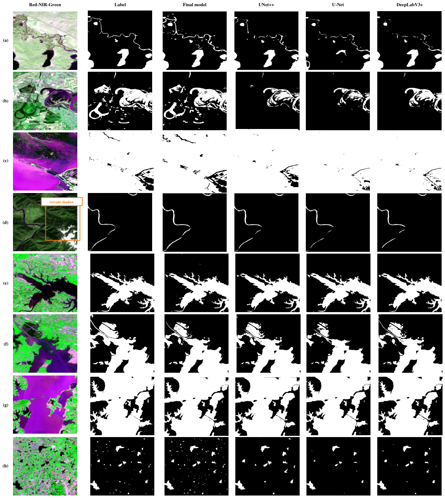
No cloud or cloud-shadow quality mask was used in training or inference; only the optical validity mask was applied. Accordingly, cloud and shadow contamination can affect individual predictions and the scene-level radiometric distributions used for percentile normalization. In Figure 4, several dark regions are more consistent with cloud shadow than with cloud cover, while the central heterogeneous region in the third case has the appearance of a wetland or vegetation–water mixture. U-Net and DeepLabV3+ are not uniformly permissive: their low overall recall indicates conservative behaviour, although they can produce local commission errors in these ambiguous dark regions.

Some baseline outputs appear locally closer to the binary reference than the final prediction. Such local exceptions are compatible with the pooled quantitative ranking because a single scene can contain mixed pixels and gradual wetland or shadow–water transitions that are difficult to represent with a binary label at the nominal WFV resolution. The same correction protocol was applied consistently, and no claim is made that the proposed configuration is locally superior at every position. Observations concerning continuity or shadow suppression are therefore treated as qualitative findings limited to the displayed examples, not as boundary- or shadow-subset metrics.

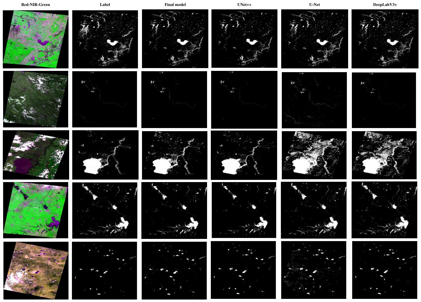
Complete-scene results reveal substantial scene-level variability within the evaluated dataset. T5 and T4 achieved the highest overlap, whereas T3 was markedly more difficult because its prediction departed from the reference over heterogeneous water-adjacent regions. T3 also showed the largest positive count bias, indicating scene-level over-extraction, while T1 and T2 showed modest negative biases and intermediate overlap. The unweighted five-scene mean was 0.915 mIoU, 0.844 Water IoU, 0.913 precision, 0.915 recall, 0.914 Water F1, and $+0.4783\%$ count bias. These complete-scene statistics extend the sampled-tile assessment but are not pooled with it because scene dimensions and water proportions differ.

Figure 5 provides the corresponding complete-scene visual comparison for T1–T5. It is used as qualitative evidence of scene-level variation and is interpreted together with the scene-level metrics rather than as a substitute for them.

Figure 5. Reference masks and complete-scene predictions for the five locked GF1/GF6 test scenes, ordered from T1 to T5 from top to bottom. Columns show the Red–NIR–Green composite, manually corrected reference, the final model, baseline UNet++, U-Net, and DeepLabV3+. The final model denotes UNet++ with RLRB and edge-consistency supervision. In the reference and prediction columns, white denotes water and black denotes background. All outputs were generated using the same seven-channel construction, valid-pixel masking, and sliding-window reconstruction protocol. The figure provides qualitative evidence only; scene-level quantitative metrics are reported separately in Table 7.

Figure 5. Reference masks and complete-scene predictions for the five locked GF1/GF6 test scenes, ordered from T1 to T5 from top to bottom. Columns show the Red–NIR–Green composite, manually corrected reference, the final model, baseline UNet++, U-Net, and DeepLabV3+. The final model denotes UNet++ with RLRB and edge-consistency supervision. In the reference and prediction columns, white denotes water and black denotes background. All outputs were generated using the same seven-channel construction, valid-pixel masking, and sliding-window reconstruction protocol. The figure provides qualitative evidence only; scene-level quantitative metrics are reported separately in Table 7.

Table 7. Complete-scene performance on the five locked test scenes. Count bias is the relative predicted-versus-reference water-pixel-count difference. The mean is an unweighted descriptive average across scenes.

Scene	mIoU	Water IoU	Precision	Recall	Water F1	Count Bias (%)
T1	0.9032	0.8283	0.9187	0.8938	0.9061	$-2.7104$
T2	0.9124	0.8392	0.9257	0.8998	0.9126	$-2.7979$
T3	0.8523	0.7243	0.8087	0.8741	0.8401	$+8.0871$
T4	0.9491	0.9052	0.9473	0.9532	0.9502	$+0.6228$
T5	0.9576	0.9208	0.9627	0.9549	0.9588	$-0.8102$
Mean	0.9149	0.8436	0.9126	0.9152	0.9136	$+0.4783$

Table 7. Complete-scene performance on the five locked test scenes. Count bias is the relative predicted-versus-reference water-pixel-count difference. The mean is an unweighted descriptive average across scenes.

Scene	mIoU	Water IoU	Precision	Recall	Water F1	Count Bias (%)
T1	0.9032	0.8283	0.9187	0.8938	0.9061	$-2.7104$
T2	0.9124	0.8392	0.9257	0.8998	0.9126	$-2.7979$
T3	0.8523	0.7243	0.8087	0.8741	0.8401	$+8.0871$
T4	0.9491	0.9052	0.9473	0.9532	0.9502	$+0.6228$
T5	0.9576	0.9208	0.9627	0.9549	0.9588	$-0.8102$
Mean	0.9149	0.8436	0.9126	0.9152	0.9136	$+0.4783$

6.4. Accuracy–Complexity Trade-Off

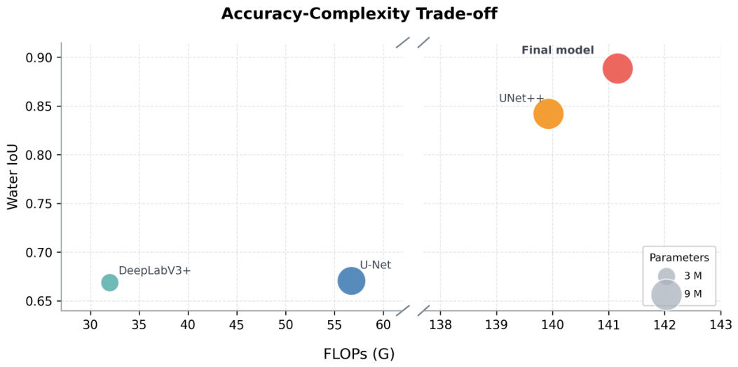
Figure 6 compares Water IoU, FLOPs, and parameter count. The final model increases the UNet++ parameter count from 9,160,866 to 9,165,540, an addition of 4674 parameters (0.051%). Measured cost increases from 139.9241 to 141.1572 G, or 0.88%. Complete-scene model forward inference required approximately 3.7 min per scene on the specified GPU under the $512\times 512$, stride-256 protocol, excluding feature construction, disk input/output, and vectorization. The modest overhead makes it unlikely that the observed change is explained solely by a substantial increase in capacity.

6.5. Practical Implications and Limitations

The feature experiment indicates that spectral indices provide the largest incremental gain over the optical-only input, while slope supplies a smaller complementary improvement in precision and overlap. RLRB and edge supervision also provide complementary gains under UNet++. However, cross-backbone validation of RLRB has not been performed, and the manuscript therefore does not claim that it is a universally transferable module. Likewise, the loss coefficients are empirically fixed settings rather than demonstrated global optima.

The model performs binary water segmentation; it does not classify water-body type, width class, size class, turbidity, or water depth. The qualitative cases are accordingly described through directly observable morphology, such as elongated water features, fragmented patches, spatially extensive regions, complex shorelines, and vegetation–water mixtures. No independent water-depth reference data were available.

The complete-scene workflow supports seven-channel input generation, weighted probability fusion across overlapping windows, NoData masking, and georeferenced outputs. Its main limitations are the concentration of acquisitions in two short 2025 warm-season windows, the fact that all five locked test scenes were acquired in May, the absence of explicit cloud and cloud-shadow masks, residual GF1/GF6 spectral-response differences without explicit harmonization, and the lack of cross-backbone testing. The current evaluation therefore characterizes scene-level spatial transfer within the available dataset rather than temporal, seasonal, or year-round generalization. Broader seasonal observations, explicit quality layers, independently documented radiometric preprocessing, and geodesic or equal-area analysis are priorities for future work.

7. Conclusions

This study developed a seven-channel UNet++ framework with residual-logit refinement for GF1/GF6 WFV surface-water extraction. The evaluation protocol locked five complete scenes, excluded non-test candidates intersecting an 8192 m spatial buffer during partitioning, and compared the learned models with the uncorrected rule-based initialization. The final configuration achieved an mIoU of 0.941, Water IoU of 0.889, and Water F1 of 0.941 on 2783 held-out tiles from the five locked scenes.

Controlled experiments showed that RLRB and edge-consistency supervision provide complementary gains under the UNet++ backbone, spectral indices supply the largest feature increment, and DEM-derived slope provides additional topographic information. The three-seed experiment characterizes only the training variability of the final configuration, and the complete-scene evaluation revealed scene-level variation that was not visible in the pooled tile-level result. RLRB adds only 4674 parameters and 0.88% measured computational cost, while average complete-scene forward inference requires approximately 3.7 min on a single NVIDIA GeForce RTX 5060 Laptop GPU. The conclusions are limited to binary surface-water segmentation and scene-level spatial transfer within the evaluated GF1/GF6 dataset; future work should examine broader seasons, explicit cloud-shadow quality layers, cross-sensor harmonization, cross-backbone transfer, and geodetically rigorous absolute-area estimation.