

Article

Satellite Remote Sensing of a Melting Glacier Albedo: Examples from EnMAP and an Intercomparison with Other Satellite and Ground Measurements


1
Department of Geography, Philipps Marburg University, 35032 Marburg, Germany
2
Helmholtz Centre for Geosciences, 14473 Potsdam, Germany
3
NASA Langley Research Center, Hampton, VA 23666, USA
4
Stevens Institute of Technology, Hoboken, NJ 07030, USA
5
Department of Environmental Science, Aarhus University, Frederiksborgvej 399, DK-4000 Roskilde, Denmark
6
National Centre for Climate Research, Danish Meteorological Institute, DK-2100 Copenhagen, Denmark
7
The Geological Survey of Denmark and Greenland, DK-1350 Copenhagen, Denmark
8
School of Earth and Environment, University of Canterbury, Canterbury 8140, New Zealand
9
Instituto de Hidráulica e Hidrología, Universidad Mayor de San Andrés, La Paz 699, Bolivia
*
Author to whom correspondence should be addressed.
Remote Sens. 2026, 18(17), 2929; https://doi.org/10.3390/rs18172929
Submission received: 19 May 2026 / Revised: 19 August 2026 / Accepted: 20 August 2026 / Published: 1 September 2026

Highlights

What is the main finding?
  • This study is aimed at the intercomparison of broadband albedo (BBA) of melting glaciers derived from multiple instruments and algorithms. It is found that various broadband glacier albedo satellite products provide similar spatial distributions. They are highly correlated. However, the derived values of BBA can differ by more than 5–10%, especially over bare land ice, which exceeds the target accuracy of 3–5%, as evidenced by the World Meteorological Organization Global Climate Observing System Program.
What are the implications of the main finding?
  • More efforts must be put into the development of highly accurate and full physics-based algorithms for the determination of glacier albedo from space that account for atmospheric correction and topography effects.

Abstract

Here, we study melting glacier surface albedo using satellite hyperspectral imagery from the Environmental Mapping and Analysis Program (EnMAP). The proposed broadband albedo (BBA) retrieval algorithm is based on radiative transfer theory and includes atmospheric and topography corrections. The comparison with ground and other satellite snow and ice albedo products is presented. Ways to improve current satellite snow and ice albedo retrieval algorithms are discussed. While the EnMAP-derived BBA is highly correlated with BBA retrieved from other spaceborne instrumentation and algorithms, the various modern snow and ice satellite BBA products can differ by more than 5–10% for snow and, especially, bare ice. Bare ice optical heterogeneity is high from variable roughness conditions and impurity content. Bare ice BBA uncertainties exceed requirements needed for highly accurate assessment of glacier climatic effects.

1. Introduction

The land surface albedo is the ratio of the solar light reflected from the Earth’s surface to the incident flux. It is a key forcing parameter controlling the partitioning of radiative energy between the atmosphere and surface [1,2,3]. Spectral and broadband (visible, near-infrared, and shortwave) albedo is an essential climate variable, which is monitored at the global scale with satellite sensors [4,5]. At present, much attention is attracted not only to the problem of the current global glacier spatial extent reduction but also to the detection of the decrease in glacier ice thickness [6] and albedo in a warming climate [3,7]. The United Nations has designated 2025 as the International Year of Glaciers’ Preservation, along with its proclamation of 21 March as the World Day for Glaciers starting in 2025, to highlight the importance of glaciers and ensure that those relying on them, and those affected by cryospheric processes, receive the necessary hydrological, meteorological, and climate services.
The spatial extent of glaciers (except debris or rock glaciers) can be monitored by optical satellite instrumentation because of the high optical contrast of bare land and snow-/ice-covered surfaces, which appear much brighter. In particular, the World Glacier Inventory [8] contains information for over 130,000 glaciers. Inventory parameters include geographic location, area, length, orientation, elevation, and classification. Additionally, the Randolph Glacier Inventory (RGI) is a global set of glacier outlines; it is intended as a snapshot of the world’s glaciers [9]. Although the spatial extent of glaciers changes with time, having the smallest spatial extent in summer, its temporal variation is not as pronounced as temporal changes in glacier albedo, which are influenced by atmospheric temperature and other atmospheric processes such as precipitation (liquid water and ice), mists and deposition of dust, soot, and other solid and liquid aerosol particles transported by atmospheric circulation. Both the spatial extent of glaciers and their albedo influence the radiative regime in respective areas. Therefore, future Glacier Albedo Inventory (GAI) must also contain the broadband albedo (BBA) as a function of both location and time. In addition, this inventory must contain the spectral albedo, which can be considered as a vector for each location in space and time. Clearly, such a worldwide snow and ice albedo inventory can be created only using multiple instruments based on various satellite platforms. Such a dataset will assist in a better understanding of both climate change and current/future sea level rise trends. An important point in this respect is the harmonization of various available snow and ice albedo global datasets derived by various algorithms from spectral solar light reflectance measured by various sensors with their specific technical parameters such as spatial resolution, spectral channel information, observation geometry, and revisit time. The first step in this process is understanding the differences between values of snow/ice albedo derived using various techniques and satellite platforms and their intercomparison with ground measurements [10,11,12,13,14,15,16,17,18].
The task of this paper is to propose the FAST semi-analytical algorithm for the determination of the spectral and broadband ALBedo (FASTALB) of melting glaciers from spaceborne satellite hyperspectral observations accounting for both the topographic and atmospheric effects. The algorithm has a high processing speed. Although the algorithm is generic in nature, it is applied to the hyperspectral Environmental Mapping and Analysis Program (EnMAP) measurements (https://www.enmap.org (accessed on 19 August 2026)), which is the German spaceborne imaging spectrometer mission. We also compare the broadband albedo derived from EnMAP with results obtained from ground-based and other satellite observations performed over a melting glacier.
The FASTALB is based on the approach proposed in [19], except that the topographic and improved atmospheric correction schemes have been added. In addition, the quality of retrieval is assessed via analysis of the root mean square difference between EnMAP spectral measurements and simulated spectra with account for the retrieved parameters for each pixel.

2. Broadband Surface Albedo

The broadband surface albedo A (also called the black sky broadband albedo) is determined by the following equation:
A = λ 1 λ 2 r p ( λ , μ 0 ) F λ d λ λ 1 λ 2 F λ d λ ,
where F λ is the bottom-of-atmosphere (BOA) incident solar light spectral irradiance, μ 0 is the cosine of the solar zenith angle, λ 1 is the initial wavelength, and λ 2 is the final wavelength used for the integration of the solar irradiance F λ at the bottom of the atmosphere (BOA), and r p ( λ , μ 0 ) is the directional–hemispherical reflectance (DHR) or spectral plane albedo defined as
r p ( μ 0 ) = 2 0 1 R ¯ ( λ , μ 0 , μ ) μ d μ ,
where μ is the cosine of the viewing zenith angle and
R ¯ ( λ , μ 0 , μ ) = 1 2 π 0 2 π R ( λ , μ 0 , μ , ϕ ) d ϕ
is the BOA directional reflectance R ( λ , μ 0 , μ , ϕ ) averaged with respect to the relative azimuthal angle ϕ . The white sky broadband albedo A W is determined in the same way as the black sky albedo A, except one needs to substitute the plane albedo by the spherical albedo in Equation (1):
r s ( λ ) = 2 0 1 r p ( λ , μ 0 ) μ 0 d μ 0 .
The blue sky albedo is defined as
A ¯ = ( 1 f ) A + f A W ,
where f is the diffuse light scattering fraction of atmospheric radiation.
In practice, one is interested in several values of the broadband albedo, which differ by limits of integration in the nominator of Equation (1) (see Table 1). The blue sky broadband albedo can be easily measured by ground-based pyranometers, which perform the 3D integration of solar light reflectance as given above in an automatic way. In particular, the pyranometer CMP21 (Kipp & Zonen, Delft, The Netherlands) performs measurements of the downward and upward (reflected) solar flux irradiances in the range 305–2800 nm and also in the range 708–2800 nm with the RG715 cut-off filter dome. This makes it possible to determine the visible, shortwave, and NIR blue sky BBA. Taking into account that the diffuse light scattering fraction is generally small over polar regions in cloud- and fog-free conditions, which is of interest for this work, the measured value is close to the black sky albedo (see Equation (5)).
The satellite measurements of BBA, being of great importance due to their global survey of worldwide glaciers, require the development of a comprehensive processing algorithms for the determination of the BOA spectral reflectance R ( λ , μ 0 , μ , ϕ ) , which can be used to derive both spectral and broadband albedo as discussed above. It should be pointed out that most satellite instruments measure the top-of-atmosphere (TOA) reflectance R T O A ( λ , μ 0 , μ , ϕ ) at a single viewing geometry ( μ , ϕ ) . Therefore, there is no essential information to perform integration as indicated in Equations (2) and (3). To avoid this problem, the correlations between BBA measured on the ground and TOA reflectances at several channels are used [13,14,15,20]. Such an approach is limited to areas where there are established networks of ground measurements [21,22]. For global satellite retrievals of BBA from space, the multiple observations of the same area from different directions during several days or even weeks are proposed [23,24,25]. This makes it possible to sample the same area from different observation directions and derive both BOA reflectance and BBA. The problem with this approach is that the surface could be drastically changed during the measurement time span due to precipitation, sudden temperature change, dust and soot aerosol deposition, etc. It should be pointed out that the usage of the geostationary observations (https://www.eumetsat.int/our-satellites/meteosat-series, last accessed on 19 August 2026) or multiple-view instrumentation [26] can partially mitigate this problem.
Yet another approach for the BBA determination has been proposed in [16]. It is based on the fact that snow reflectance is determined by the ice grain sizes, shapes, wetness, and pollution load [27]. For the case of glacier ice modeled as polluted bubbly ice, the size of bubbles and concentration of various pollutants are the main drivers of the spectral reflectance change [28,29,30]. Therefore, solving the inverse problem and determining respective local optical and microphysical parameters of snow and glacier ice from TOA spectral reflectance makes it possible to reconstruct the complete BOA reflectance and, therefore, determine both spectral and broadband albedo using satellite measurements of top of atmosphere (TOA) reflectance [11,12,16,29]. Following this approach, one can make more accurate spectral integrations, as shown in Equation (1), because the function R ( λ , μ 0 , μ , ϕ ) can be derived at any wavelength and not only at fixed channels as it is done in the traditional approach [23]. Also, in this advanced approach, no multiple observations of the same area are needed, and the whole glacier broadband albedo can be determined exactly at the time of measurements, which is a clear advantage over the traditional approach. Moreover, other albedo values, such as white sky and blue sky broadband albedo values, can be determined.

3. The Retrieval of Glacier Ice and Snow Albedo Using Asymptotic Radiative Transfer Theory

In this work, we improve the broadband and spectral snow and glacier ice albedo algorithm proposed in [19], accounting for topographic effects. The algorithm is based on asymptotic radiative transfer and finds that the snow and glacier ice reflection function depends mainly on just four spectrally neutral parameters, both for snow and glacier ice.
These four spectrally neutral parameters can be considered as intrinsic characteristics of snow and glacier ice, respectively. Clearly, they determine not only the reflectance but also the broadband albedo, which is an integral of reflectance with respect to the wavelength and angular variables as discussed above. Therefore, the retrieval of albedo is reduced to the determination of four intrinsic parameters from single-view satellite measurements of spectral snow and glacier ice reflectance. Importantly, such an approach does not rely on either on multiple observations of a given target from different angles or any assumption on the microstructure parameters of snow and glacier ice (e.g., the size, shape and nature of light scattering centers), which is of clear advantage as compared to other techniques, especially those used for the characterization of complex random media, such as snow and glacier ice.
In particular, it has been shown that the BOA glacier reflection function R s u r f , black sky albedo, r p and the white sky albedo r s can be modeled using the following analytical expressions [19,31]:
R s u r f = a R exp α λ L R ,
r p = a p exp ( α ( λ ) L p ) ,
r s = a s exp ( α ( λ ) L s ) ,
where
α ( λ ) = α i c e ( λ ) + κ p o l ( λ ) ,                           κ p o l ( λ ) = κ 0 λ / λ 0 b ,
L R = ε R 2 L ,       L p = ε p 2 L ,       L s = ε s 2 L ,
ε R = ε s + b ( ξ , η ) 1 ,       ε p = ε s + u ( ξ ) 1 ,   ε s = ( 1 r l ) 1 ,
b ( ξ , η ) =   u ( ξ ) u η R 0 1 ξ , η ,           u ( ξ ) = 3 7 1 + 2 ξ ,
R 0 ξ , η is the solar light reflection function of a semi-infinite nonabsorbing layer of snow or glacier ice (after passing light through the air ice interface), ξ = 1 ( 1 μ 0 2 ) / n i c e 2 is the cosine of the solar zenith angle after penetration through the air–ice surface with the bulk ice refractive index n i c e , η = 1 ( 1 μ 2 ) / n i c e 2 is the cosine of the viewing zenith angle measured below the interface, α i c e ( λ ) is the bulk ice absorption coefficient, L is the effective absorption length, κ p o l ( λ ) is the function, which is proportional to the absorption coefficient of pollutants characterized by the Angström exponent b and the parameter κ 0 κ p o l ( λ 0 ) proportional to the load of pollutants, and r l is the internal diffuse reflection coefficient at the boundary glacier surface–air for the light coming from below. This coefficient is equal to zero for the case of snow, where the respective boundary is absent. In this particular case, Equations (6)–(12) transform to similar equations for snow [27].
The parameters a R , a p , and a s give the values of the reflection function, plane albedo, and spherical albedo for the case of nonabsorbing media ( α L 0 ). The derivation of four spectrally neutral parameters ( a R , L R , b , κ 0 ) from spectral reflectance can be performed using either the optimal estimation [10,11,12] or the analytical approach proposed in [27].
In this work, we shall determine the values of a R , L R , as proposed by [19]. Namely, it is assumed that the measurements in near-infrared are not affected by either snow pollutants or atmospheric effects. In this case, the sought parameters can be derived from measurements at two NIR channels ( λ 1 , λ 2 ) and Equation (6). Namely, it follows [19]:
a R = R s u r f σ ( λ 1 ) R s u r f 1 σ ( λ 2 ) ,                                 L R = C ln 2 R s u r f ( λ 2 ) R s u r f ( λ 1 ) ,
where
C = λ 2 4 π χ 2 ,                                                   σ = 1 λ 2 χ 1 λ 1 χ 2 1 ,
R s u r f ( λ j ) is the surface light reflectance at the wavelength λ j and χ j is the imaginary part of the complex refractive index of ice at the wavelength λ j . In this work, we suggest using the wavelengths λ 1 = 880 and λ 2 = 1048 nm, where it is possible to ignore the influence of both atmospheric effects and snow impurities on registered spectra. One can find that χ 1 = 3.35 × 10 7 and χ 2 = 2.204 × 10 6 in this case [32,33] and, therefore, σ = 1.74 ,   C = 65.86   mm .
For the case of polluted surfaces, two other parameters ( b ,   κ 0 ) must be determined. They are found using the approach proposed in [19,34]. Namely, one can ignore the absorption by ice in the visible. Then, it follows from Equation (6) that at two wavelengths in the visible region:
R s u r f ( λ 1 ) = a R exp κ p o l λ 1 L R ,   R s u r f ( λ 2 ) = a R exp κ p o l λ 2 L R .
Subsequently, one derives:
b = 2 ln z ( λ 1 / λ 2 ) ,           z = ln ( R s u r f ( λ 2 ) / a R ) ln ( R s u r f ( λ 1 ) / a R ) ,         κ 0 = L R 1 λ 1 λ 0 b ln 2 R s u r f ( λ 1 ) a R .
In particular, the EnMAP channels located in the visible region of the electromagnetic spectrum at 424 and 492 nm have been used in this work. In the case of neutrally spectral reflectance in the visible region, it follows that:
κ p o l = L R 1 ln 2 R s u r f ( λ 1 ) a R .
It should be pointed out that, unlike for the case of near-infrared measurements, one should account for atmospheric light scattering effects in the determination of parameters (b, κ 0 ). This has been done as discussed below.
We use the following approximation for the measured TOA reflectance [19,34,35]:
R m e a s ( λ ) = R a t m ( λ ) + R s u r f ( λ ) T a t m ( λ ) 1 r s ( λ ) r a t m ( λ ) T g a s ( λ ) ,
where atmospheric characteristics R a t m ( λ ) , T a t m ( λ ) , T g a s ( λ ) , and r a t m ( λ ) are calculated using the information on the spectral atmospheric optical thickness, as discussed in [17]. They are defined in Table 2.
The value of R s u r f ( λ ) can be derived from Equation (18) analytically:
R s u r f ( λ ) = R m e a s ( λ ) R a t m ( λ ) T ( λ ) + ( R m e a s ( λ ) R a t m ( λ ) ) r a t m ( λ ) ,
where we assumed that T g a s ( λ ) = 1 at the selected wavelength λ and r s ( λ ) R s u r f ( λ ) . The latter equation is valid only for Lambertian surfaces. However, the introduced error is negligible because atmospheric optical thickness in polar regions is small and, therefore, the last term in the denominator of Equation (18) is close to zero. Equation (19) is used in Equations (16) and (17) to evaluate the glacier surface parameters ( b , κ 0 ).
The derived parameters ( a R , L R , b , κ 0 ) make it possible to determine the BOA reflectance at each spectral channel using Equations (6) and (9). The determination of the black sky spectral albedo from BOA reflectance can be performed using the following formula, which follows from Equations (6) and (7):
r p = a p R s u r f ( λ ) a R m ,
where m = ε p / ε R . Let us estimate the parameter m assuming isotropic light scattering in glacier ice. Then, it follows that [36]:
R 0 1 ξ , η = 4 ξ + η H ( ξ ) H η ,
where [37]
H ( ξ ) = 4 u ( ξ ) 3
for the case studied. It follows from Equation (18) that:
b ( ξ , η ) = 3 4 ξ + η .
Therefore, one derives:
m = ε s 1 + 3 7 1 + 2 ξ ε s 1 + 3 4 η + ξ .
It follows that for typical observation conditions (say, ξ = 1/2, η = 1), the value of m only weakly depends on ε s , which is of clear advantage because of uncertainties related to the determination of this parameter for real-world glacier surfaces.
One can derive the glacier spherical albedo as well:
r s = a s r p / a p n ,
where
n = ε s ε s 1 + 3 7 1 + 2 ξ .
Equation (20) makes it possible to determine black sky spectral albedo directly from the values of the glacier reflectance R performed from a single observation direction, assuming that the internal reflection coefficient r l and the parameter a p are known. In this work, we take the value of r l = 0.454 [38,39] for flat surfaces with a refractive index of 1.31 (ice in the visible) and a ratio of Υ = a p / a R = 1. As explained above, for typical nadir satellite observations, the parameter m only weakly depends on r l . Therefore, it is not expected that our results will be considerably influenced by the choice of r l . The parameters a p and a R represent plane albedo and nadir reflectance of a glacier surface at no absorption. Generally, these parameters are different for smooth surfaces. However, taking into account that glacier surfaces are very rough, one can expect that these characteristics are close and ϒ 1 . The rough surface randomizes the angular distribution of escaped photons, acting as an effective diffuse plate, which is used to measure the plane albedo of glaciers in the field campaigns [19].
The same procedure can be applied for the white sky albedo. The broadband albedo (either white sky or black sky) can be derived using numerical integration, as given by Equation (1).

4. The Topographic Correction

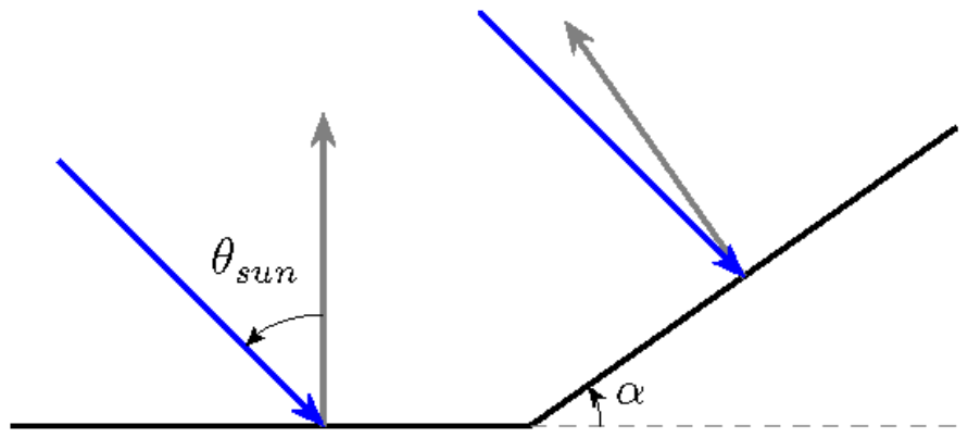
The plane albedo depends on the local incidence angle and, therefore, on the topography of the surface (Figure 1). The inclined glacier surface with the slope α in Figure 1 is illuminated by the sun at the solar zenith angle close to zero (almost nadir illumination), which makes it less reflective as compared to the horizontal glacier surface at the bottom illuminated by the sun with the solar zenith angle θ s u n . This is due to the fact that it is easier for the photons at oblique incidence to escape from the glacier underneath as compared to the case when photons penetrate the glacier along the perpendicular to the surface. In the last case, photons undergo more multiple light scattering and absorption events as compared to the case with θ s u n 0 . Therefore, they have smaller probabilities to survive the interaction with the surface and be reflected, leading to the darker appearance of the glacier, even if the optical properties of the horizontal and inclined glacier surfaces (see Figure 1) are absolutely the same. Thus, the glacier surface slope effect cannot be ignored. The situation with the reflection function is even more complicated because of the need to calculate not only the local incidence angle γ s u n but the local observation angle γ v i e w and the local relative azimuth Φ .
It is clear from our analysis that the information on local solar incidence and observation angles is essential for the determination of the glacier plane albedo. Although such information is readily available while performing ground measurements, where the nadir observation conditions can be easily secured, this is a more difficult task requiring a digital elevation model (DEM) and the extracted surface slope and aspect. In this work, we have used the European Space Agency DEM at a 30 m spatial resolution to estimate the slope α and aspect β of the surface [40] using:
tan 2 α = p 2 + q 2 ,   tan β = q / p ,
where
p = d z d x , q = d z d y
and (x,y,z) are the rectangular coordinates with z positive up, y positive to the north, and x positive to the east.
The slope and aspect of the tilted surface can be used to derive the local (at the tilted snow surface) solar zenith angle γ s u n and the local viewing zenith angle γ v i e w [41,42,43] via:
cos γ s u n = cos θ s u n cos α + sin θ s u n sin α cos ( φ s u n β ) ,
cos γ v i e w = cos θ v i e w cos α + sin θ v i e w sin α cos ( φ v i e w β ) .
The local relative azimuthal angle Φ can be easily derived from the invariance of the scattering angle with respect to the surface tilt [41]:
cos θ s u n cos θ v i e w + sin θ s u n sin θ v i e w cos ( φ s u n φ v i e w ) = cos γ s u n cos γ v i e w + sin γ s u n sin γ v i e w cos Φ .
The TOA spectral radiance is taken here from the EnMAP L1C data. We use the tabular data for the solar irradiance at the top of atmosphere E 0 provided in [44] to derive the spectral reflectance at the TOA:
R m e a s = π I m e a s u r e d E 0 cos θ s u n ,
where I m e a s u r e d is the TOA radiance as measured by the satellite instrument. We calculate the measured TOA reflectance using an approximation:
R s i m ( λ , θ s u n , θ v i e w ) = R a t m ( λ , θ s u n , θ v i e w ) + R s u r f ( λ , γ s u n , γ v i e w , Φ ) T a t m ( λ , θ s u n , θ v i e w ) 1 r s ( λ ) r a t m ( λ ) T g a s ( λ , θ s u n , θ v i e w ) ,
where
R s u r f = π I B O A ( γ s u n , γ v i e w , Φ ) E 0 cos γ s u n ,
and I B O A ( γ s u n , γ v i e w , Φ ) is the BOA reflectance of the inclined glacier surface. Equation (33) with the term R s u r f defined by the angles γ s u n , γ v i e w , and Φ (see Equation (34)) is used by us for the solution of the inverse radiative transfer problem for the case of tilted glacier surfaces by substituting the radiative transfer problem for a tilted snow surface by a well-known radiative transfer problem for a flat vertically and horizontally homogeneous surface with a modified term R s u r f . It should be pointed out that atmospheric radiative transfer characteristics listed in Table 1 are defined for the black underlying surface. Therefore, the change in angular variables in these terms is not needed. Equation (33) transforms to the standard equation for the horizontal surface at the inclination angle equal to zero.
The influence of the neighborhood (adjacency effects) for the case studied in this work is negligible and, therefore, the respective term is absent in Equation (33), as has been done in the popular Atmospheric/Topographic CORrection for satellite imagery software [45].

5. The Application of the Algorithm for the Retrieval of Broadband Albedo Using EnMAP Hyperspectral Measurements

Let us apply the algorithm described above to the satellite hyperspectral measurements over melting glaciers in southern Greenland. Although the algorithm can be used for any hyperspectral instrument orbiting the planet at present, we concentrate on retrievals using the Environmental Mapping and Analysis Program (EnMAP), which is a German hyperspectral mission that monitors and characterizes the environment of the Earth on a global scale. The instrument measures the reflected solar radiance in the spectral range 418–2450 nm (224 channels) with a spatial resolution of 30 m. Further details on the instrument and its applications are given in [46] We have used EnMAP L1C radiance data provided by the German space agency (DLR) in a range of latitudes of 65.5–65.9N and longitudes of 38.4–39.4W (6 September 2025, 14:51:13UTC). The reflectance was calculated from the EnMAP L1C radiance using Equation (32). In most cases, the reflectance is in the range 0–1, with smaller values for bare ground and ocean. Before the application of the BBA retrieval algorithm, we have sorted pixels with respect to the underlying surfaces using thresholds given in Table 3.
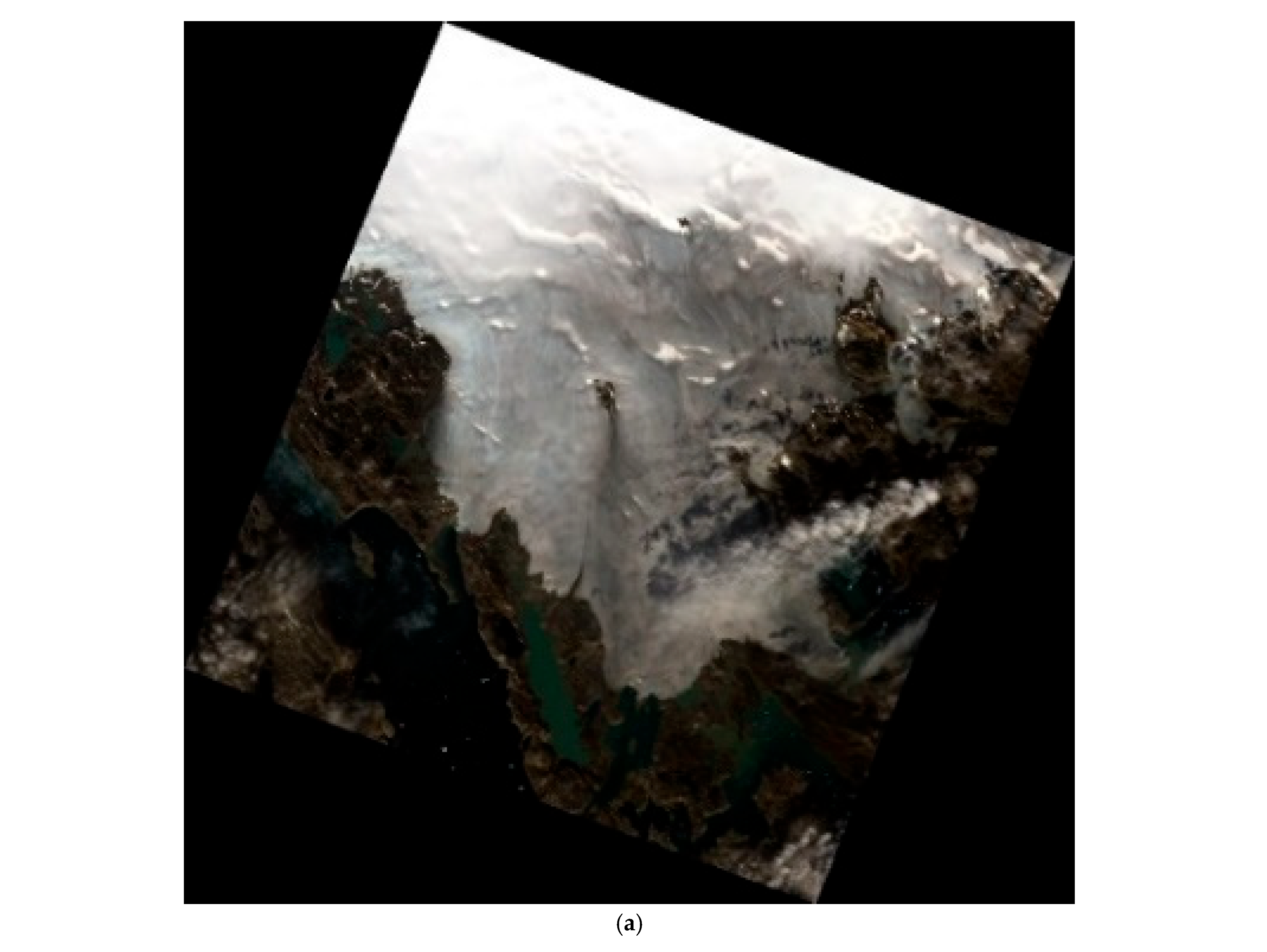
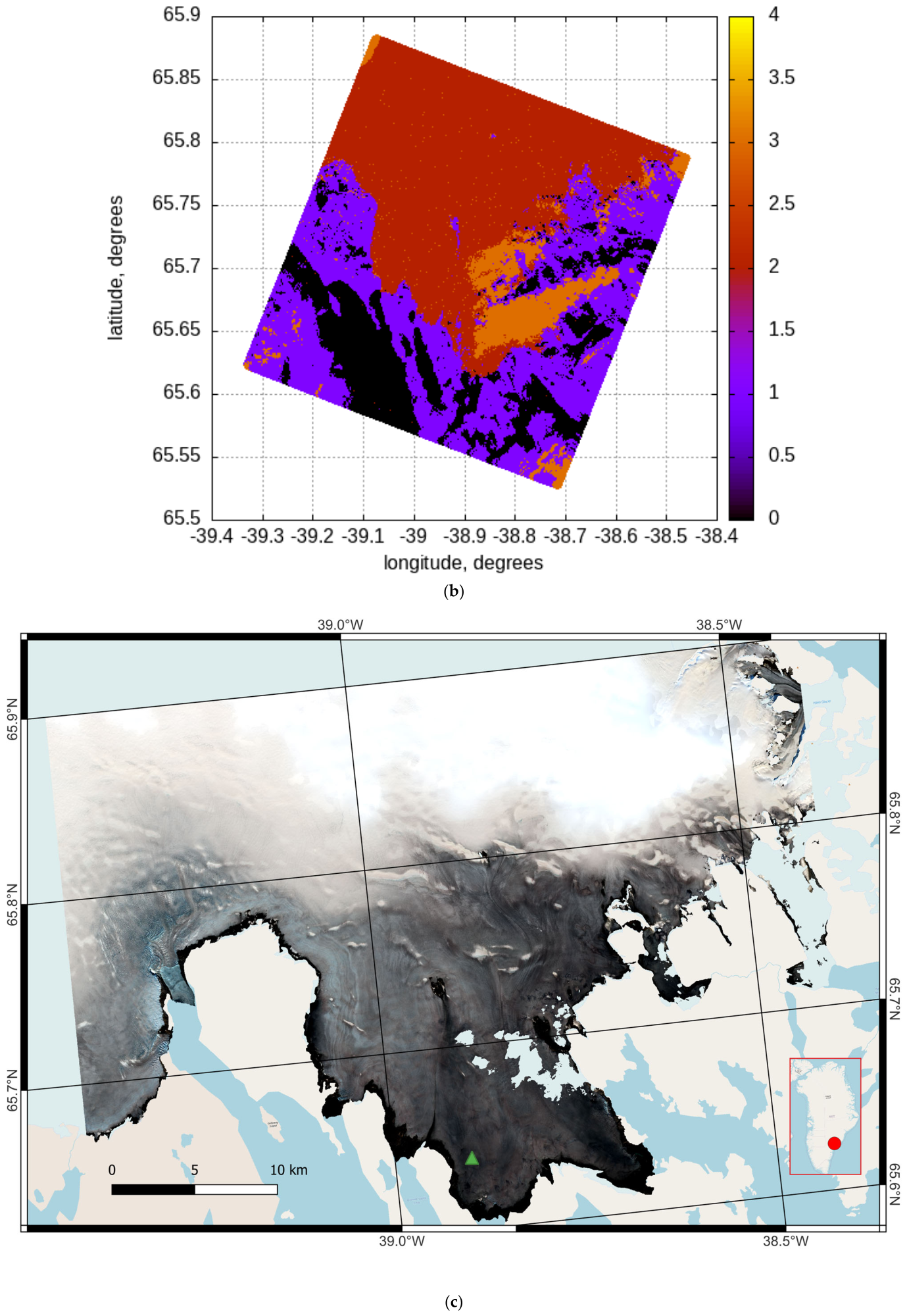
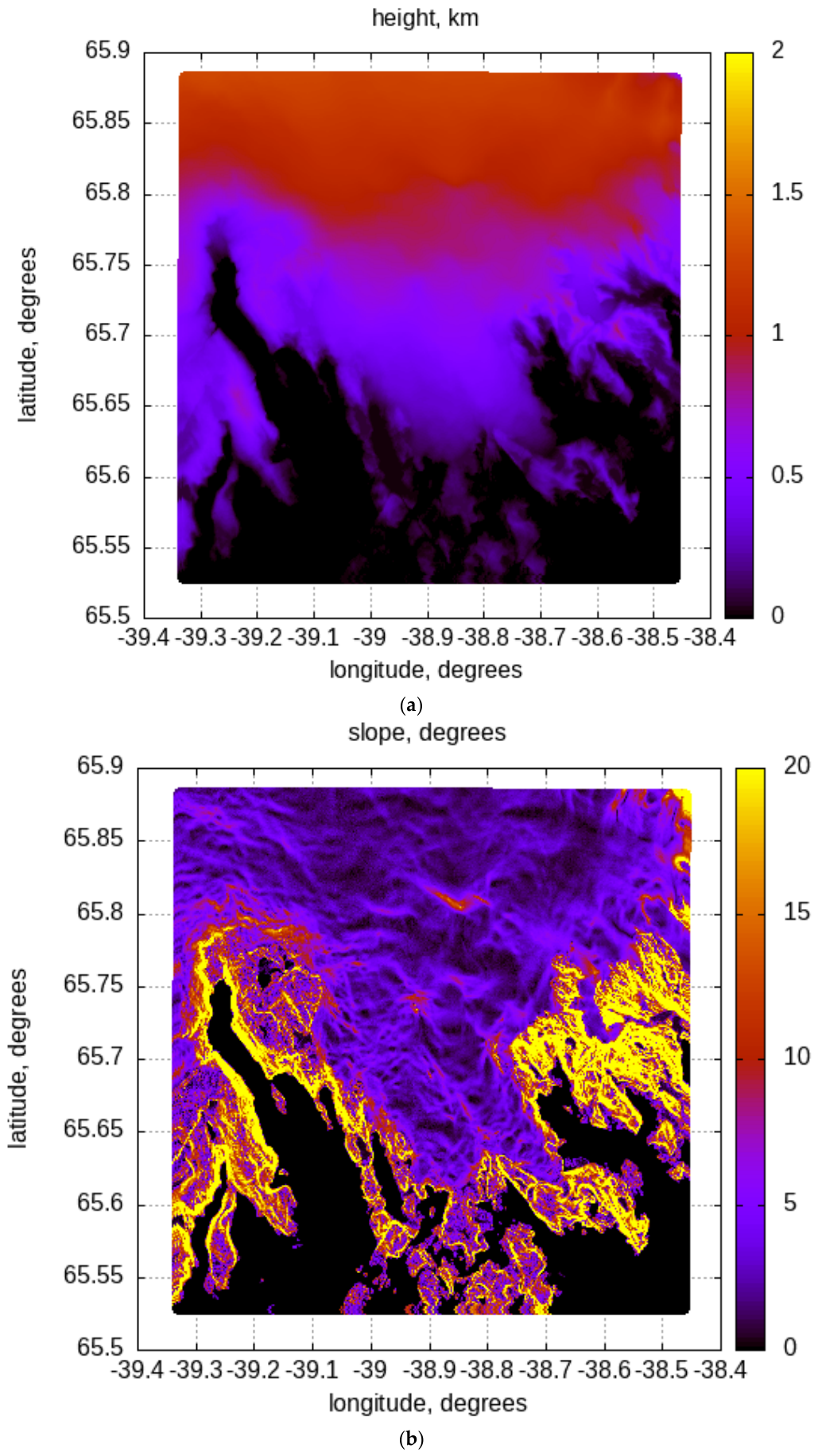
The illustration of the performance of the pixel identification algorithm together with the respective EnMAP and S-2 browse images appears in Figure 2. The analysis of Figure 2 suggests that the performance of the algorithm is satisfactory for our task related to the BBA determination for snow and bare ice areas. The spatial distribution of surface height (Figure 3a) and the derived slope distribution (Figure 3b) show that the surface height decreases toward the ocean, with slopes remaining below 5° across most snow and bare ice EnMAP pixels. Therefore, significant topographic effects on the retrieved albedo are not expected. This is particularly important for comparisons with other satellite albedo products with no topographic correction.
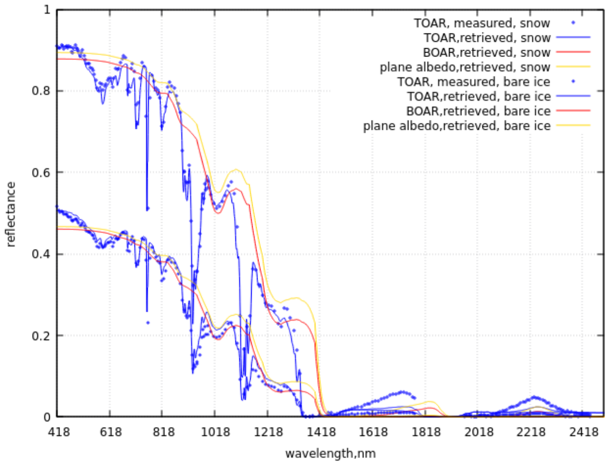
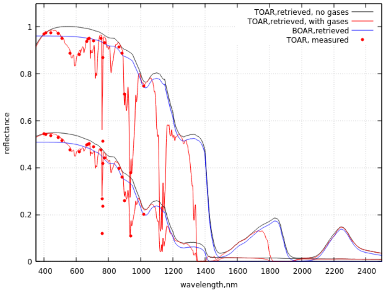
The algorithm makes it possible to derive not only the BOA reflectance (BOAR), but also one can find spectral plane albedo and reconstruct the TOA reflectance (TOAR), as demonstrated in Figure 4 for the two selected EnMAP pixels. We have used the vertical columns of water vapor and ozone provided in the respective L1C EnMAP file. In the calculations of the TOA reflectance, we have assumed that the spectral aerosol optical thickness can be described by the Angström law
τ a ( λ ) = τ a ( λ 0 ) ( λ / λ 0 ) ν ,
where λ 0 = 550   nm and ν is the Angström exponent. The Arctic atmosphere is usually clean with small values of the aerosol load and optical thickness [34]. Therefore, we have varied the aerosol optical thickness τ a ( 550   nm ) in the range 0.04–0.1 for a single pixel to minimize the normalized root mean square difference (NRMSD)
Λ = 1 N j = 1 N R j , s i m R j , m e a s 2 1 N j = 1 N R j , m e a s
and assume that the derived AOT does not change considerably on the scale of the EnMAP 30 × 30 km scene.
It should be pointed out that the retrievals are not based on the optimal estimation technique and some parameters (such as aerosol Angström exponent ν = 1.2) are assumed before the retrieval starts. Therefore, we do not minimize the NRMSD for all pixels and rather provide it in the output of the algorithm to understand the quality of retrievals. This makes it possible to increase the speed of calculations considerably and improve the retrievals using postprocessing, if necessary. We have selected the value of N = 110 in Equation (36). This means that reflectance values at λ > 1100   nm have not been accounted for in the NRMSD calculations.
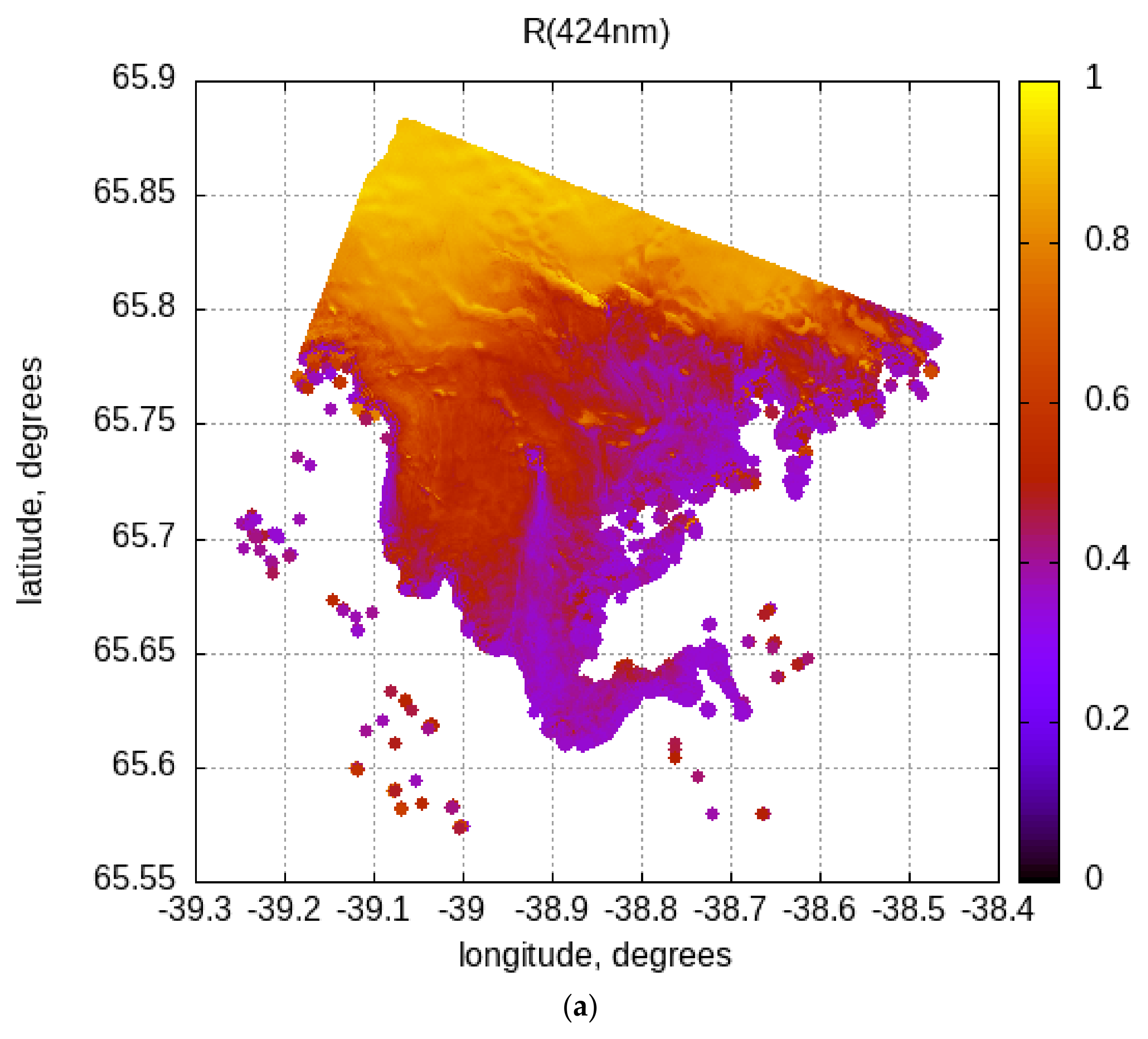
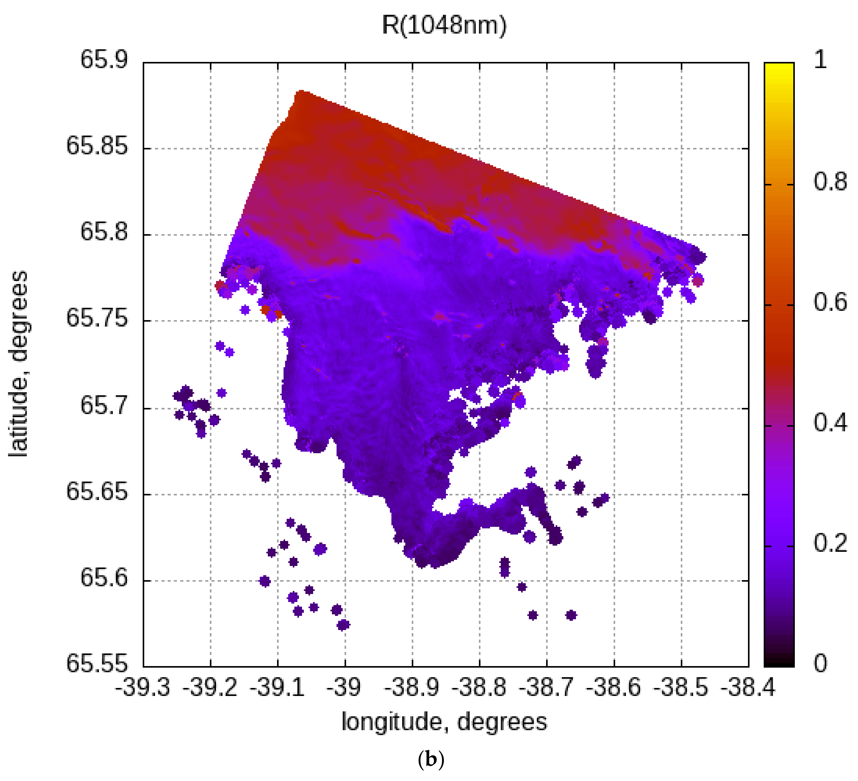
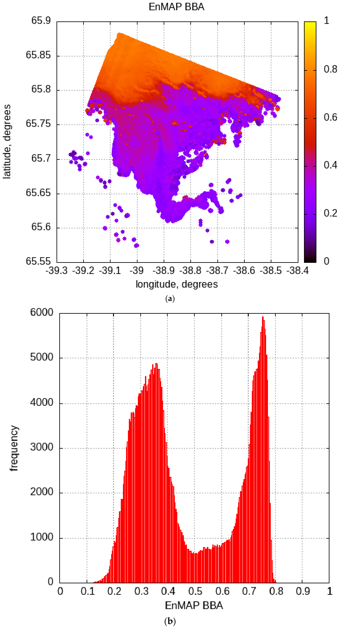
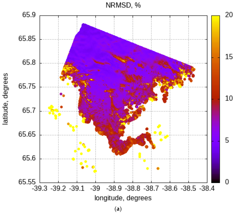
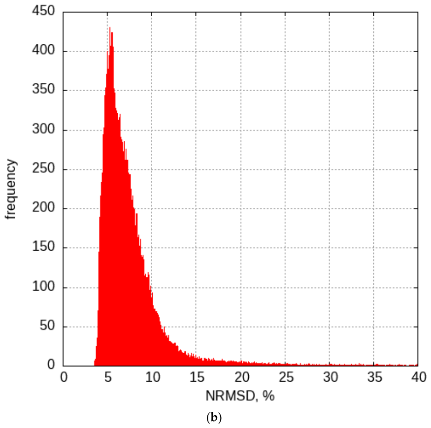
The EnMAP reflectances at 424 and 1048 nm are shown in Figure 5. The derived black sky BBA and its frequency distribution are given in Figure 6. The derived values of BBA for glacier ice and snow as derived by FASTALB appear reasonable. The BBA distribution is characterized by modes at 0.35 and 0.75 for glacier ice and snow, respectively. The spatial distribution of the normalized RMS differences calculated for the EnMAP spectral range 418–1048 nm appears in Figure 7 and is in the range 5–12% for most of the retrievals.
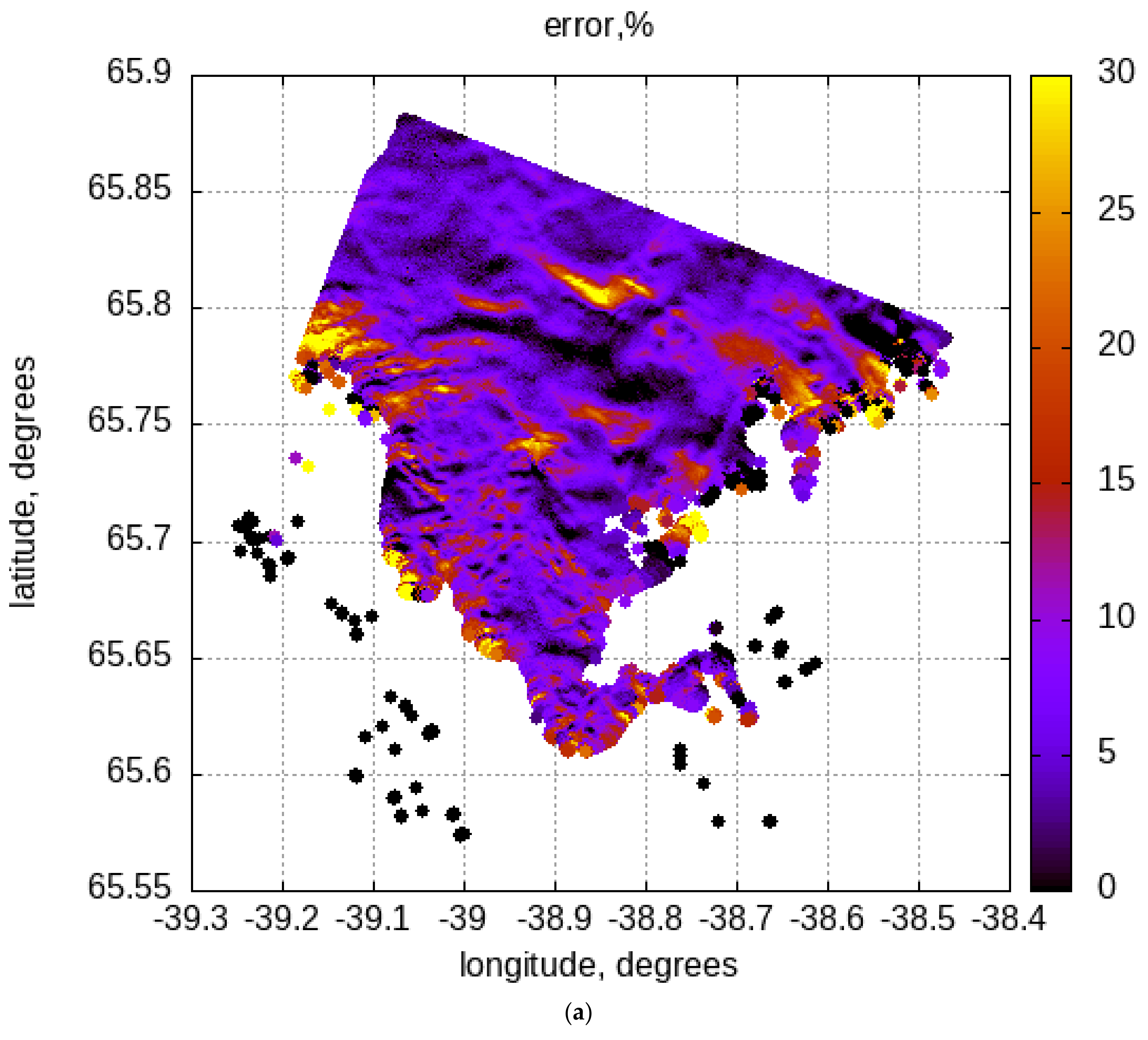
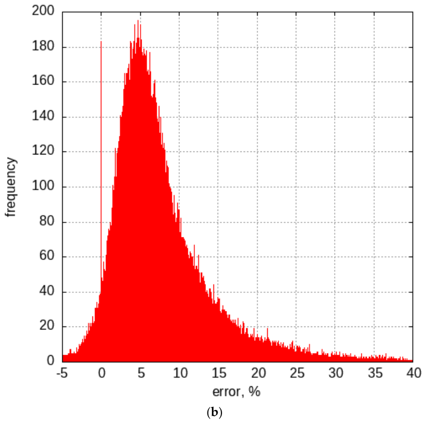
The spatial distribution and histogram of the relative BBA error (assuming zero surface slope) for the inclined glacier surface are shown in Figure 8. Neglecting the surface slope results in an overestimation of the glacier surface albedo by ~5% on average, consistent with the positive mean relative error. Generally, the influence of slopes on the BBA is very much reduced as compared to the influence of slopes on spectral reflectance and albedo (especially in ice absorption bands). The part of the error in the BBA calculations without accounting for slopes is not only due to an incorrect assumption on local incidence and observation angles but also due to the inaccuracy of the effective length determination for a sloppy terrain (see Equation (13)), especially in the case of bare ice surfaces.
The retrieved values of BBA are next intercompared with retrievals from other satellite missions and ground measurements at a single location in Greenland.

6. The Intercomparison of the Derived Broadband Albedo with Other Satellite BBA Products and Ground Measurements

6.1. The Comparison of Snow and Ice BBA Retrievals Performed by Multiple Spaceborne Instrumentation

6.1.1. The Description of Satellite Instruments and Algorithms

Validation of satellite-derived broadband albedo against ground measurements requires expensive field campaigns, often conducted under harsh conditions. In contrast, comparing BBA retrievals from different satellite instruments is relatively straightforward, although it remains limited by the availability of cloud-free observations.
In this section, we compare the derived EnMAP shortwave black sky broadband albedo with the respective values obtained from other spaceborne sensors. The main goal is to understand the consistency of the retrieval algorithms. The respective instruments and retrieval algorithms (except the EnMAP algorithm already described above) are now briefly introduced. The spatial collocation has been performed in the way described in [47].
OLCI/S-3
The Ocean and Land Colour Instrument (OLCI) [48] is a push-broom instrument sharing the field of view (FOV). The FOV of OLCI’s five cameras has a fan-shaped configuration in the vertical plane, perpendicular to the platform velocity. It records top-of-atmosphere radiance at 21 channels in the 400–1020 nm wavelength range. We used the Sentinel-3 Greenland snow and ice broadband albedo product SICEv3.0 (https://dataverse.geus.dk/dataset.xhtml?persistentId=doi:10.22008/FK2/7POQG5 (accessed on 19 August 2026)), where the snow albedo is computed using a fast atmospheric correction technique [17] and bare ice albedo is estimated via a simple linear regression between OLCI TOA and PROMICE albedo measurements [20]. In SICEv3.0 [49], bare ice is separated from snow using the bare ice onset albedo threshold of 0.565 [20]. The snow spectral albedo retrieval algorithm is based on the asymptotic radiative transfer theory. The BBA for snow is derived using Equation (1). The spatial resolution of the product is 500 m. Further details are given in [17].
SGLI
The Second Generation Global Imager (SGLI) was launched with the JAXA GCOM-C1 satellite in December 2017. The instrument acquires data in 19 spectral channels from 0.38 to 12 µm and includes polarization measurements in selected channels (https://www.eorc.jaxa.jp/JASMES/SGLI_NRT/index.html (accessed on 19 August 2026)). The SGLI ground spatial resolution is 250–1000 m, depending on the channel. Although the spatial resolution of the official SGLI snow albedo product is 1000 m, special processing at a resolution of 250 m has been performed for the scene studied in this work. The optimal estimation algorithm has been used [11,12]. It combines (i) a first guess from the machine learning technique, (ii) a fast Levenberg–Marquardt optimal estimation step, and (iii) posterior uncertainty analysis. The snow albedo and associated albedo uncertainty are calculated from retrieved snow parameters. The snow grain shape is approximated by the aggregated nonspherical Voronoi particles [50]. It has been found that at the Greenland SIGMA-A site, blue sky albedo retrievals agree within a root mean square difference (RMSD) = 0.048 and mean absolute percentage error = 3.3% compared to in situ measurements. Comparisons with albedo measured by the Greenland Climate Network (GC-NET) at Summit have an RMSE and MAPE of 0.035 and 3.6%. The current version of the algorithm is not valid for the bare glacier ice surfaces, and an enhanced version to rectify this problem is currently under development.
MODIS/TERRA
The Moderate Resolution Imaging Spectroradiometer (MODIS) (https://modis.gsfc.nasa.gov/) captures data in 36 spectral bands ranging in wavelength from 0.4 μm to 14.4 μm and at varying spatial resolutions (two bands at 250 m, five bands at 500 m, and 29 bands at 1 km). The NASA MODIS MCD43A1 product provides three model weighting parameters (isotropic, volumetric, and geometric) that describe the BRDF to characterize the anisotropic reflectance of the land surface [51]. These parameters are used to derive the integrated black sky and white sky albedos of various surfaces, including ice and snow [24]. They are provided daily for each MODIS spectral band at a 500 m spatial resolution and represent the best estimates from 16 days of surface reflectance data collected by the Terra (MOD09GA) and Aqua (MYD09GA) satellites, centered around the specific day of interest [25].
The bare ice and snow albedo used in this study was obtained from the NASA Terra satellite through the MOD10A1 broadband albedo product version 6.1 [52].
Landsat and MSI/S-2
We have used two BBA retrieval algorithms for Sentinel-2. They are described below.
  • Harmonized Landsat and Sentinel-2 product (HLS)
We utilized analysis-ready surface reflectance data from the NASA Harmonized Landsat and Sentinel-2 product (HLS) [53]. This product combines data from the Landsat 8 and 9 Operational Land Imager (OLI) and the Sentinel-2A/B/C MultiSpectral Instrument (MSI) sensors (https://www.earthdata.nasa.gov/data/instruments/sentinel-2-msi (accessed on 19 August 2026)) and applies a consistent set of algorithms for atmospheric correction, cloud and cloud–shadow masking, geographic co-registration, common gridding, bidirectional reflectance distribution function (BRDF) normalization, and bandpass adjustment to generate a seamless surface reflectance record. The black sky and white sky albedos in MODIS spatial resolution at HLS solar-view geometries are needed for the HLS S-2 product. Therefore, the MCD43A1 data were obtained from the NASA Earthdata Search engine (https://search.earthdata.nasa.gov/) accessed on 6 September 2025 in the area of interest. The BRDF is calculated for each spectral band using the Ross Thick-Li Sparse Reciprocal semi-empirical model [54]:
  B R D F θ v i e w ,   θ s u n ,   φ ,   λ = f i s o λ +   f v o l λ K v o l θ v i e w ,   θ s u n ,   φ + f g e o ( λ )   K g e o ( θ v i e w ,   θ s u n ,   φ )  
where φ is the relative azimuthal angle, Kvol and Kgeo are the prescribed volumetric and geometric kernels, respectively, and fiso, fvol, and fgeo are the isotropic, volumetric, and geometric parameters derived from 16 days of MODIS observations of the same target area in the absence of clouds. The volumetric and geometric kernels are calculated using the equations described in [54], with the HLS sun and view angles expressed in radians. The black sky and white sky albedos in MODIS spatial resolution at HLS solar-view geometries are calculated using the following polynomial approximations:
r p θ s u n , λ = f i s o λ ( g 0 i s o + g 1 i s o × θ s u n 2 + g 2 i s o × θ s u n 3 )   + f v o l λ ( g 0 v o l + g 1 v o l × θ s u n 2 + g 2 v o l × θ s u n 3 ) + f g e o ( λ ) ( g 0 g e o + g 1 g e o × θ s u n 2 + g 2 g e o × θ s u n 3 )
r s λ = f i s o ( λ ) × g i s o + f v o l ( λ ) × g v o l + f g e o ( λ ) × g g e o
where the coefficients gjk are listed in [24]. Finally, the spectral black sky and white sky albedos are transformed to broadband albedos using the conversion coefficients developed in [55].
S-2 surface reflectance data were downloaded for 6 September 2025 from the NASA Earthdata Search engine (https://search.earthdata.nasa.gov/). They included two scenes recorded at 13:53:56 and 14:14:13, respectively, which contained all seven spectral bands and a quality assessment layer with cloud masks, and information on the geometry of observations. First of all, the reflectances R at the following bands were extracted for processing: blue (0.45–0.51 μm), green (0.53–0.59 μm), red (0.64–0.67 μm), near-infrared (NIR, 0.85–0.88 μm), the shortwave infrared bands 1 (SWIR 1, 1.57–1.65 μm) and 2 (SWIR 2, 2.11–2.29 μm); the cloud masks; the sun zenith angle; the sun azimuth angle; the view zenith angle; and the view azimuth angle. These bands were clipped to the area of interest, and the cloud mask was used to screen clouds and cloud shadows. In HLS, the surface reflectance products are normalized for a nadir view by applying the c-factor approach [56]. However, this method is not applicable for generating albedo. Thus, the nadir-view reflectance was divided by the c-factor to obtain non-view-angle-corrected surface reflectance.
After calculating these quantities, the spectral albedo-to-nadir reflectance ratios γ are determined for both black sky albedo and white sky albedo at HLS solar-view geometries in MODIS spatial resolution:
γ p θ s u n , λ = r p θ s , λ / B R D F θ v i e w ,   θ s u n ,   φ ,   λ
γ s λ = r s λ / B R D F θ v i e w ,   θ s u n ,   φ ,   λ
Next, HLS data is reprojected to the MODIS sinusoidal projection, aggregated to 500 m spatial resolution, and then a cluster-based unsupervised classification is performed. The ratios γ calculated with Equations (40) and (41) are sampled for homogeneous pixels covered by more than 60% of the same cluster class, and the mean of all >60% class-specific γ ratios is applied to the HLS pixels classified as the respective cluster class to obtain medium-resolution black sky and white sky albedo:
r p ,   H L S θ s , λ = γ p θ s , λ R θ s , θ v , φ ,   λ
r s ,   H L S λ = γ s λ R θ s , θ v , φ ,   λ .
Finally, the spectral black sky and white sky albedos are transformed to broadband albedos using the conversion coefficients developed in [55].
  • Ice surface optimized, harmonized Landsat and Sentinel 2 product (ICEHLS)
In addition, an ice surface optimized, harmonized Landsat and Sentinel 2 (S2) dataset (ICEHLS) was used to derive S2 albedo for the study area. The dataset applies cross-sensor calibration to harmonize S2 using Landsat 8/9 imagery as the reference image, following the workflow adapted from [56,57]. It ensures radiometric consistency across sensors and improves temporal sampling for glacial environments. Cloud and cloud–shadow contamination were removed using the weakly supervised, deep learning-based Cloud Score+ product [58] implemented in Google Earth Engine [59], which has demonstrated improved performance over traditional cloud masking methods. We used the visible and near-infrared (NIR) bands from the S2 components of the ice surface-optimized, harmonized Landsat and Sentinel 2 dataset to take advantage of high spatial resolution (10 m) after harmonization. Broadband albedo was then computed using the narrow-to-broadband conversion algorithm described in [13]. This algorithm was originally developed for the Greenland Ice Sheet and has been validated in glacier environments across the Arctic and in alpine settings, yielding correlation coefficients ranging from 0.68 to 0.92 [14]. The resulting albedo product, therefore, represents spatially consistent, atmospherically corrected, surface broadband albedo suitable for assessing seasonal and interannual variability in glacier surface conditions. In the comparisons, we have used a 30 m spatial resolution version of the product.

6.1.2. The Intercomparison of Broadband Albedo Retrieved from Multiple Satellite Retrieval Algorithms

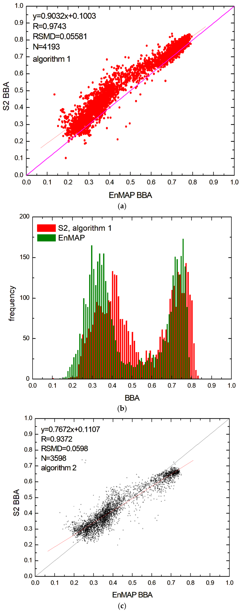
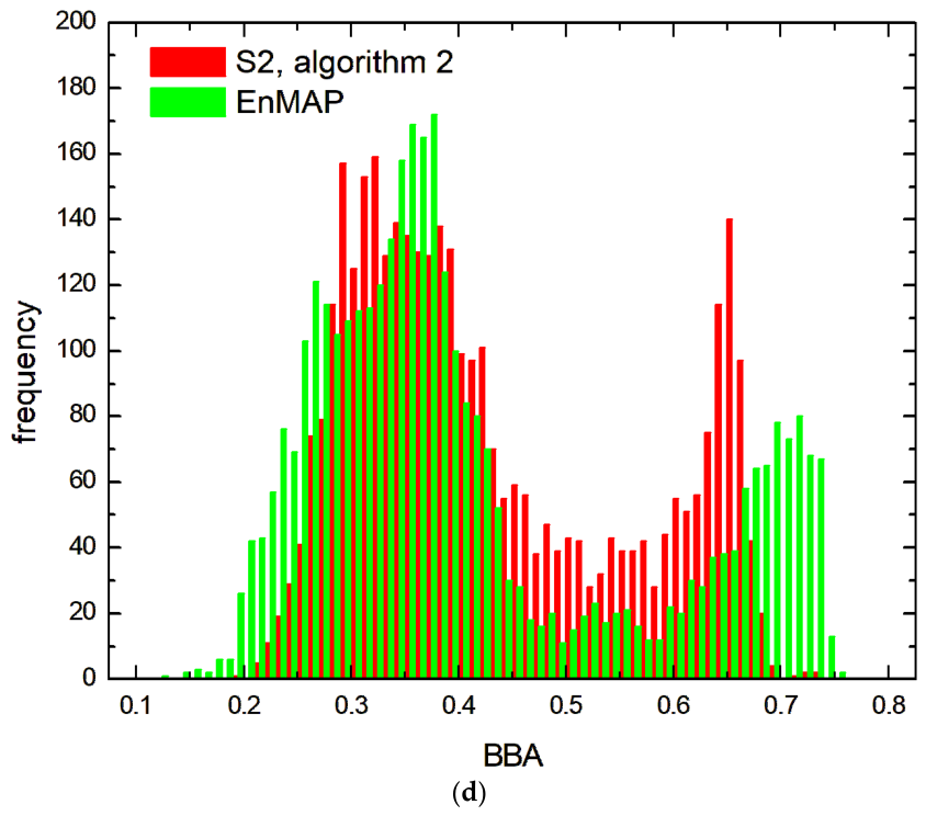
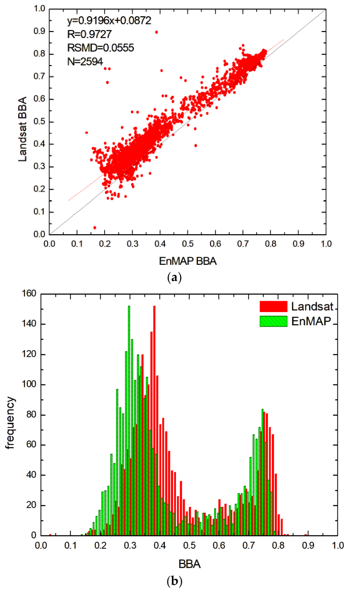
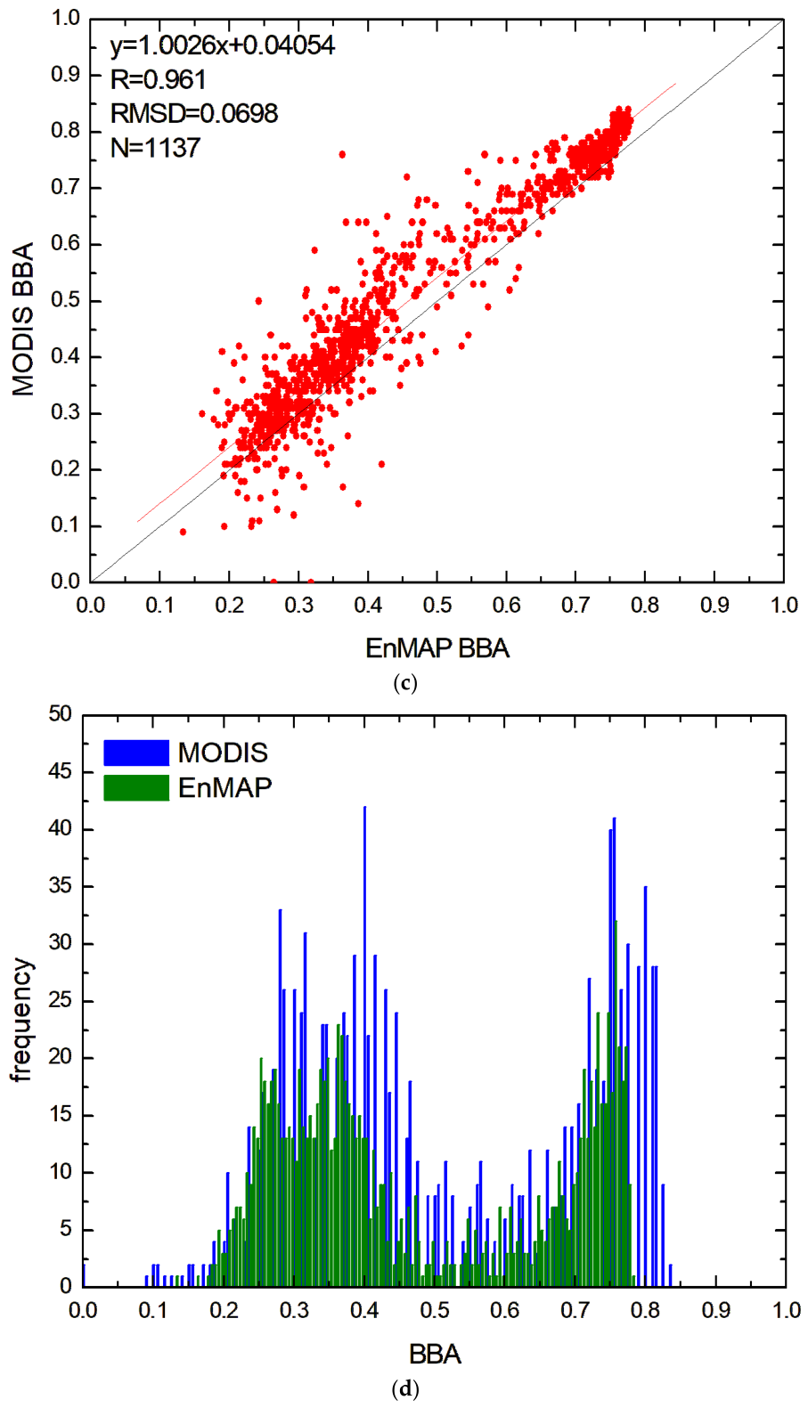
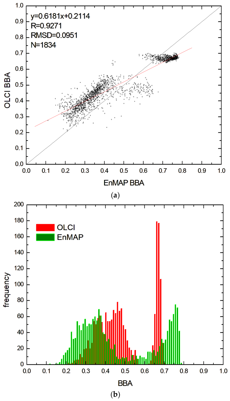
Correlation plots of various satellite BBA products versus the EnMAP BBA are presented in Figure 9, Figure 10 and Figure 11. All products show high correlation, with OLCI/S3 exhibiting modestly lower values, especially in the snow–ice transition region (BBA 0.4–0.6) and over wet snow (BBA > 0.6). It follows that the values of BBA derived from various instruments and algorithms do not differ considerably, with somewhat smaller values of BBA as derived from EnMAP. This is not necessarily a drawback of the EnMAP algorithm because it has been found that the BBA values derived from MODIS, S2, and Landsat are biased high as compared to ground measurements [15]. The statistical parameters related to the intercomparison studied reported above are given in Table 4.
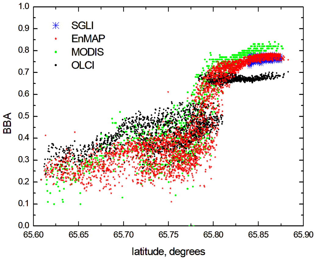
The latitudinal dependence of BBA derived from EnMAP and other satellites appears in Figure 12. We have found that the average black sky BBA for the part of the image covered by snow is 0.778 according to EnMAP. It is equal to 0.766 according to spatially and time-collocated SGLI data. The difference is below 2%, which confirms the consistency of both retrieval techniques over snow-covered areas. MODIS and OLCI have positive and negative biases as compared to EnMAP and SGLI for the snow-covered part of the image. All instruments show an increase in snow albedo with latitude, as one may expect.
An important point to understand is the variability of the glacier albedo derived from different instruments for the same area. We have selected two areas—one is covered by melting snow (65.83–65.84N; 38.9–39W), and another is covered primarily by glacier ice (65.75–65.76N, 38.72–38.82W) for 6 September 2025. The results of average black sky SW BBA retrievals for these areas appear in Table 5. One can see that EnMAP, SGLI, MODIS, and S-2 HLS algorithms produce roughly equivalent results for the black sky SW BBA, with differences below 6%. The Landsat measurements are absent for this specific area on 6 September 2025. The derived values of albedo provided by OLCI and MSI/S-2 ICEHLS algorithms are about 10% smaller than the EnMAP retrievals. Although the differences are relatively small, they exceed the maximal error range (5%) in the respective satellite product recommended by GCOS, if the results derived from OLCI and MSI/S-2 ICEHLS algorithms are taken into account. Otherwise, the consistency of the products is almost in the range proposed in [60] (just a 6% difference among four independent instruments and algorithms).
The situation is more complex for the observations over bare glacier ice, where the derived values of the BBA are in the range of 0.30–0.45, depending on the sensor. The relative bias with respect to EnMAP measurements is in the range of [−13%, 24%], which is clearly outside GCOS requirements. Therefore, the reason for the differences between respective algorithms over melting glaciers must be understood and reduced with possible improvements of the BBA retrieval strategies. Again, the results derived from EnMAP, MODIS, and S-2 HLS algorithms are relatively close (the absolute difference below 0.06). The difference between Landsat and EnMAP measurements is about 0.04. The current version of the SGLI algorithm cannot be applied to the glacier ice regions. OLCI and S-2 ICE HSL algorithms give the largest differences from the EnMAP results with the BBA in the range of 0.43–0.45.
Summing up, the derived values of BBA are in the range of 0.67–0.78 (16% difference) and 0.3–0.45 (50% difference), which is well outside GCOS requirements of 5% [60]. Such a large variability of the results derived from various satellite platforms points to the fact that not all algorithms can be used, for instance, for albedo temporal trend studies. Also, the fusion of the results derived from multiple satellite platforms is in question.
Differences in retrieved broadband albedo (BBA) are not caused solely by variations in spatial and spectral resolution or the number of spectral channels among satellite instruments. The specific design and assumptions of the individual retrieval algorithms applied to the same dataset also play a significant role. In particular, the OLCI snow algorithm is based on radiative transfer modeling developed for dry snow conditions. This may partly explain the biases observed in this study when compared with EnMAP hyperspectral retrievals, which are more representative of melting snow. Additionally, these algorithms use different atmospheric correction techniques, and not all of them consider surface anisotropy. The correction for surface anisotropy is different for snow and ice.
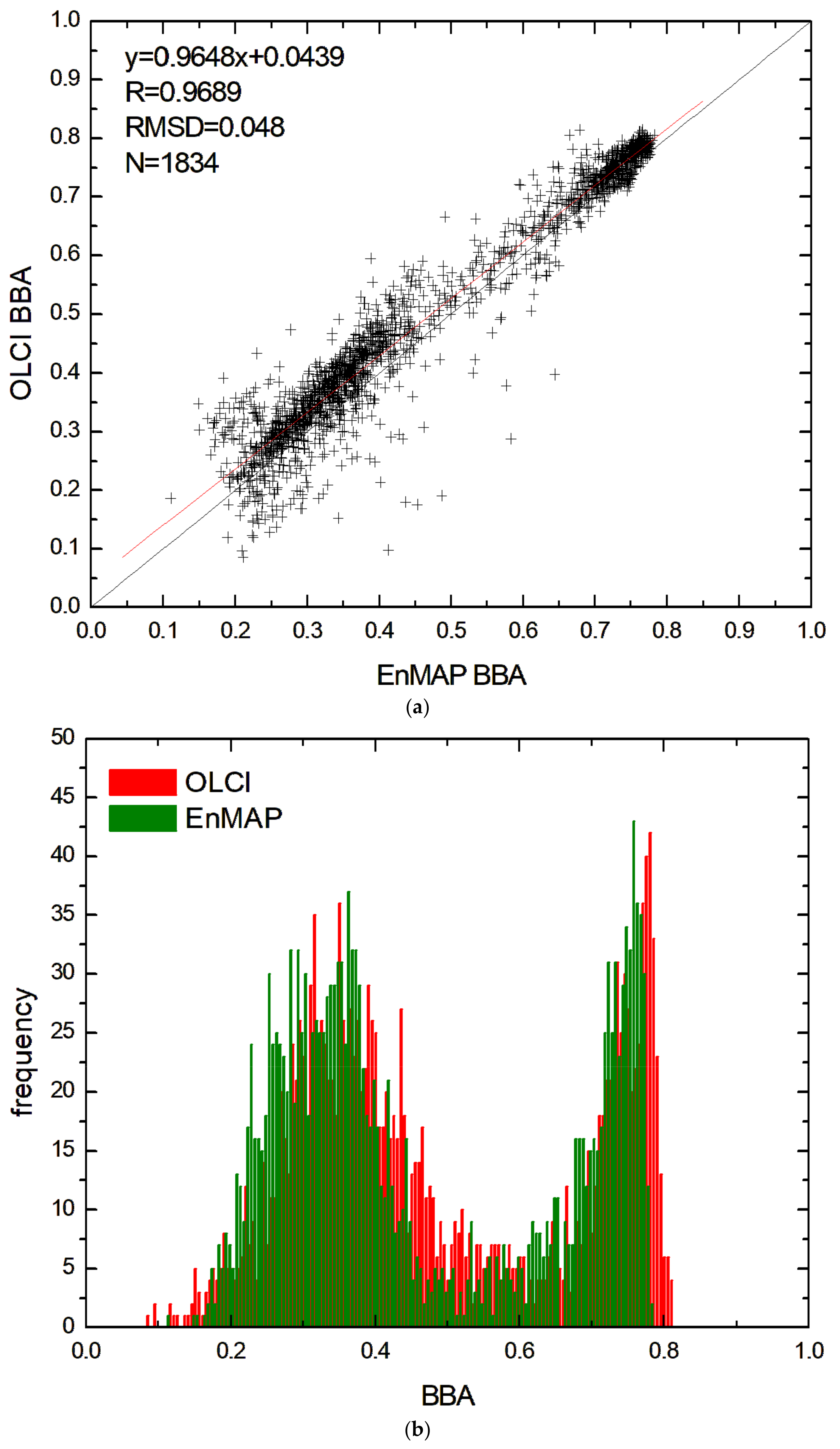
To test this hypothesis, we applied the EnMAP retrieval algorithm (described above) to the OLCI data. The following four OLCI channels have been used in the retrievals: 400 nm, 510 nm, 865 nm, and 1020 nm, which are close to the channels used for EnMAP retrievals (424 nm, 492 nm, 880 nm, 1048 nm). The results given in Figure 13 have been derived not for the native OLCI spatial resolution (300 m) but rather for the re-processed 500 m spatial resolution OLCI dataset [49]. Therefore, our retrievals have been performed for the 500 m spatial resolution product as well. The results of BBA retrievals derived from OLCI and EnMAP using the same algorithm (except for a slightly different number of channels) are shown in Figure 13. One can see that the results are highly correlated. The small bias and scatter of the results can be explained by the inhomogeneity of the surface, the different spatial resolution of instruments, and not 100% coverage of OLCI pixels (especially at the edges) by EnMAP BBA retrievals. The intercomparison of measured OLCI spectra with those simulated using the same approach as used in the results given in Figure 4 is presented in Figure 14. One can see that the retrieved surface characteristics can be used to explain all details of the measured OLCI spectra (except those inside the oxygen A-band influenced by the OLCI smile effect not accounted for in the simulation software).

6.2. Ground Measurements

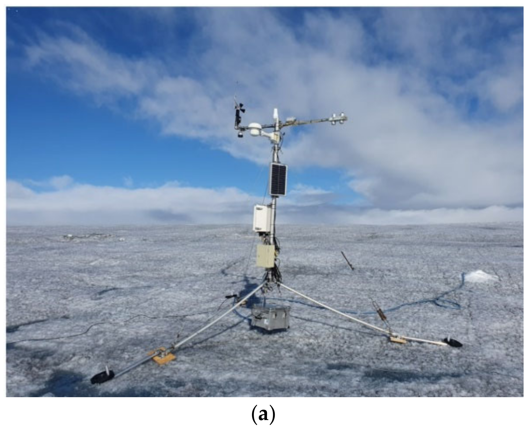
In this section, we compare the EnMAP-derived broadband albedo (BBA) with ground-based measurements acquired on 6 September 2025 at the Programme for Monitoring of the Greenland Ice Sheet and Greenland Climate Network (PROMICE) automatic weather station TAS_L (65.6390°N, 38.8993°W) [21,22]. A photograph of the station taken on the same day (Figure 15a) shows that, although the sun was not obscured by clouds directly above the station, nearby clouds were present at the time of acquisition. These clouds may have affected the quality of the ground measurements.
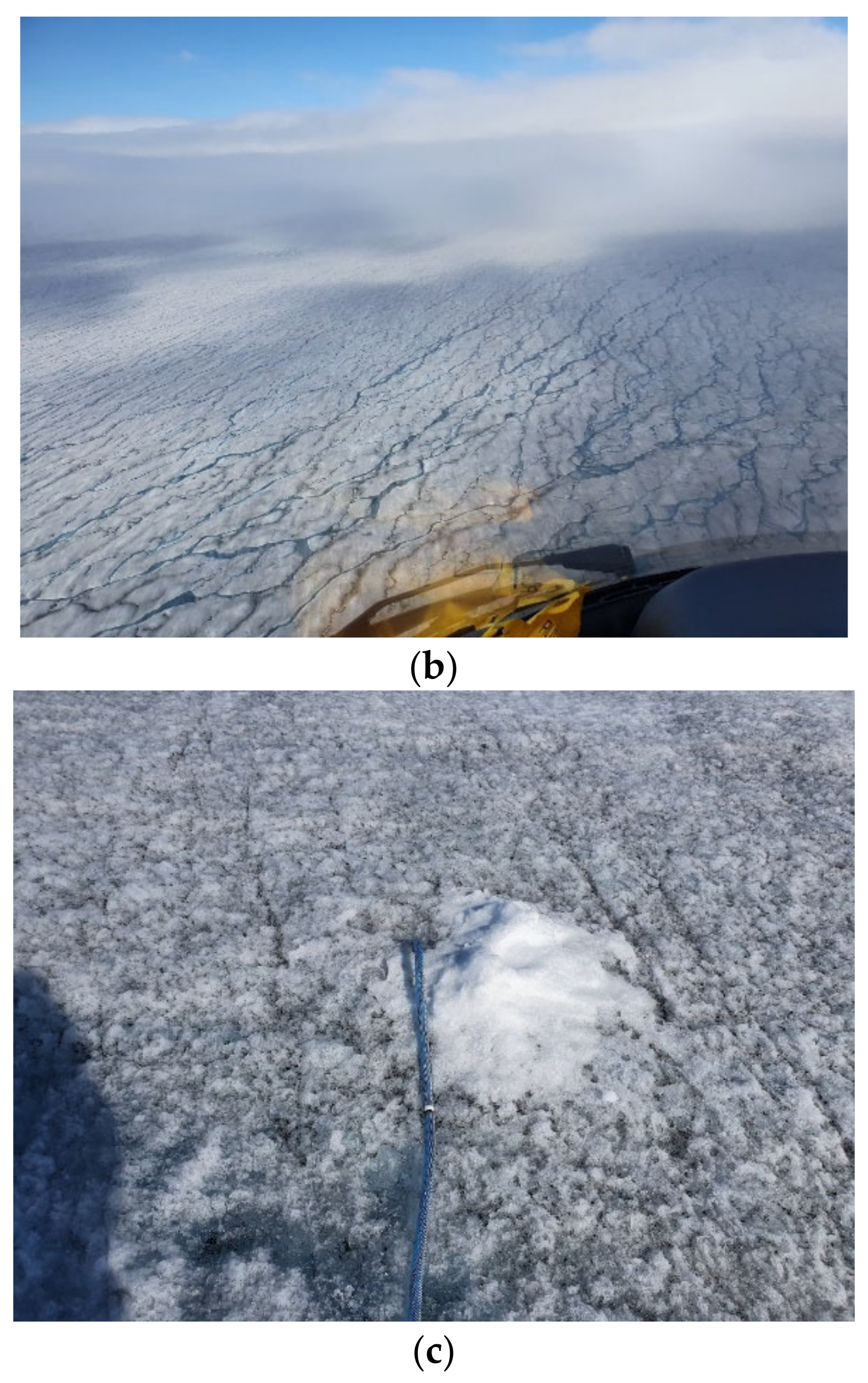
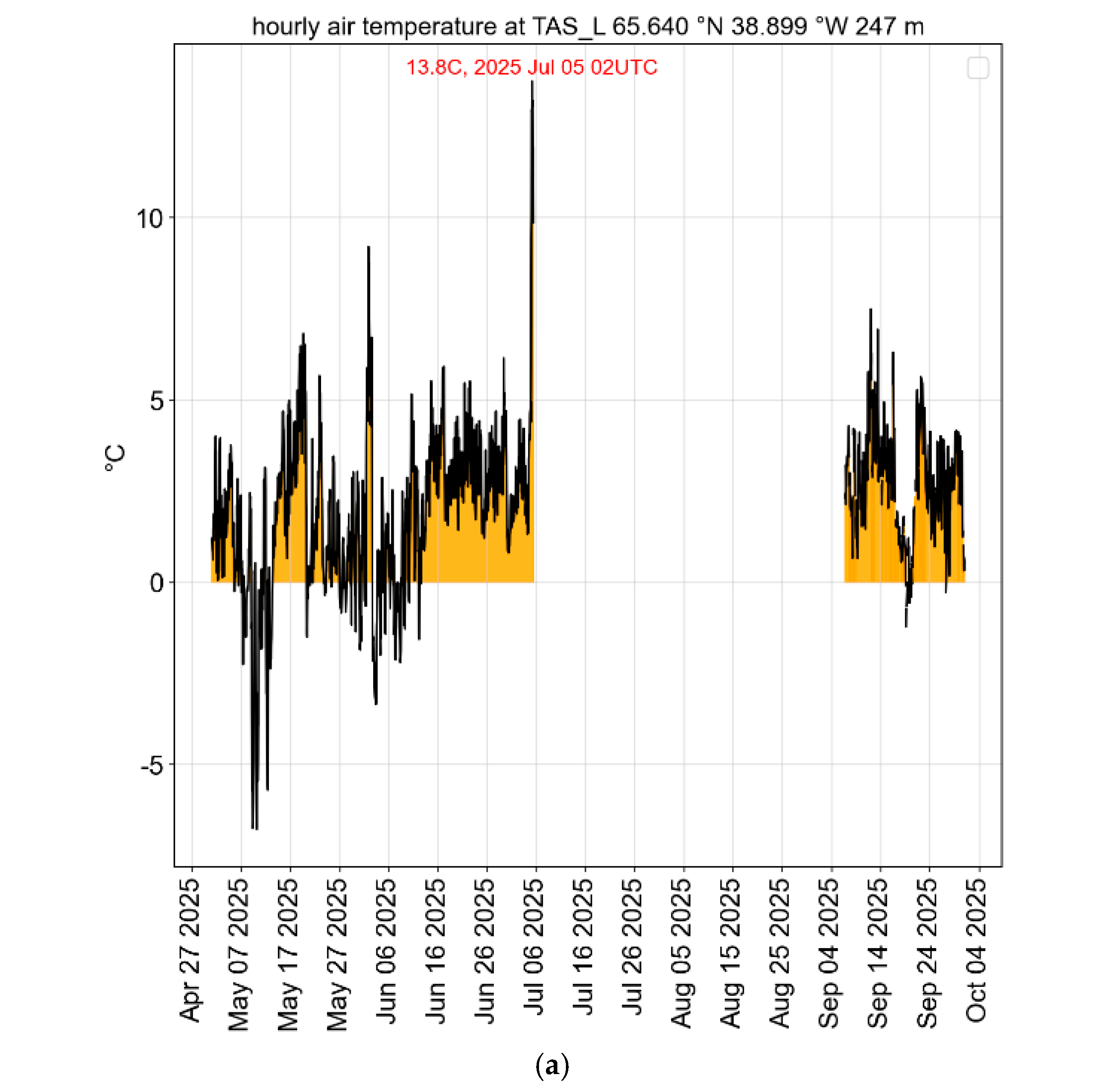
An aerial photo of the glacier surface structure taken at the time of satellite measurements around the station in Figure 15b indicates a network of water channels on the glacier ice surface, which may influence the accuracy of retrievals. These water channels are absent directly at the station (see Figure 15c). It follows from Figure 15c that dark material is present on the ice surface. Those are primarily dispersed cryoconites, which consist of mineral dust, organic matter, and microbes (like cyanobacteria). It is the biology that produces a material to “glue” those together and form their habitats, called biologically active impurities [61,62,63,64,65,66].
The temporal changes of the ground-measured and S2-derived BBA and temperature at the station are given in Figure 16. The station recorded that air temperatures were above 0 °C at the station from the middle of June until the end of September 2025. It follows both from satellite and ground observations that the value of BBA drops from the values around 0.85 at the start of the melting season at the end of May to the values around 0.3 at the peak of the melting season at the end of June. As follows from the analysis of the PROMICE database, the BBA was around 0.28 on 6 September 2025 (noon).
The satellite missions used in the intercomparisons at the TAS_L location are given in Table 6 together with the retrieved values of BBA, their spatial resolution, and the measurement time on 6 September 2025. One can conclude that the measurements with instruments having higher spatial resolution (S2, EnMAP, and Landsat) give the absolute difference with ground measurements smaller than 0.02. The time difference (except for MODIS) was just within 3 h from solar noon. Therefore, we may neglect possible changes in the snow and glacier ice temporal evolution.
It follows from the data shown in Table 6 that although retrieved and ground-measured BBA over the glacier ice do not differ by more than 13% from the ground value, there is a considerable scatter among retrievals from different instruments for the glacier ice case. Therefore, the usage of BBA from different satellites for the glacier albedo temporal changes must be taken with caution. Also, one should take into account that the spatial area for the BBA measurement at the ground (2 m 2 ) is ca. four orders of magnitude smaller as compared to the size of the satellite pixel. Therefore, the results shown in Table 6 cannot be considered as a true validation due to the inhomogeneity of the glacier ice surfaces.
The surface albedo belongs to the essential climate variables, which shall be monitored with an accuracy of 5%, with a horizontal resolution of 250 m as the minimum requirement to be met as outlined by the World Meteorological Organization Global Climate Observing System GCOS [60]. The ideal requirement is 3% error and 10 m spatial resolution. One can see that S2, Landsat, and EnMAP provide the results (for the single location) close to the ideal combined GCOS requirements of a high spatial resolution and accuracy. However, dedicated ground-based campaigns collocated in space and time domains with satellite measurements are urgently needed to quantify the accuracy of satellite retrievals over bare ice—also taking into account the error of ground measurements, e.g., due to the error in the vertical pointing of the instrument and the influence of the instrument shadowing effects. Some differences could be due to the fact that PROMICE network measurements provide the blue sky BBA, which is not the case for satellite measurements given in Table 6.
The results provided by OLCI/S3 and MODIS are given for the orientation only and cannot be considered as final ones because of sharply different spatial scales (2 m for ground measurements and 500 m for satellite measurements). In this case, the ground footprint (2 m × 2 m = 4 m2) is ~4.8 orders of magnitude smaller than the satellite footprint (500 m × 500 m = 250,000 m2). This difference in footprint is of special importance for inhomogeneous surfaces, such as the melting glacier studied in this work (see Figure 15).

7. Conclusions

We applied a modified version of the snow and glacier ice broadband albedo (BBA) retrieval algorithm proposed in [19] to EnMAP data acquired over a melting Greenland glacier, where surface albedo ranged from 0.2 to 0.8. The modifications included terrain slope correction, improved atmospheric correction, and an updated conversion from reflectance to albedo that accounts for the internal diffuse reflection coefficient and an additional free parameter.
An important avenue for future work is the empirical determination of this parameter pair from simultaneous spectral reflectance and albedo measurements over different glacier surfaces. For fresh snow, these parameters are known by definition.
At the PROMICE station TAS_L, the EnMAP-retrieved BBA over bare ice was 0.30, slightly higher than the ground measurement of 0.28. This difference is consistent with the large-scale mismatch between the satellite pixel (30–500 m) and the ground footprint (2 m), as well as possible instrument pointing and shadowing effects.
The EnMAP BBA retrievals were compared with products from Landsat, Sentinel-2, MODIS, OLCI, and SGLI. All products showed high correlation with EnMAP-retrieved BBA. The somewhat lower correlation obtained for OLCI can be attributed to (1) the relative simplicity of its bare ice algorithm (which uses top-of-atmosphere reflectance and only two fitting parameters) and (2) the known limitations of the OLCI snow algorithm for melting snow conditions.
Direct validation against ground measurements remains challenging due to the infrequent revisits of EnMAP over PROMICE stations. Nevertheless, the initial results presented here for bare ice and melting snow in Greenland, together with previous snow BBA retrievals over Concordia Station in Antarctica [67], are encouraging. A comprehensive, long-term validation effort is the subject of ongoing work.
A key finding of this study is that current satellite snow and ice albedo products can differ by more than 5–10% over snow and, especially, ice-covered surfaces. While such differences may be acceptable for some applications, they exceed the GCOS target accuracy of 5% (with a spatial resolution requirement of ≤250 m). The most stringent GCOS goals are 10 m spatial resolution and 3% absolute accuracy. We conclude that several modern algorithms (including those applied to EnMAP, SGLI, MODIS, Landsat, and Sentinel-2) produce mutually consistent results. However, dedicated ground validation campaigns—ideally supported by drones and autonomous systems—are urgently needed, despite the logistical difficulties posed by polar environments. Correlation with other satellite products is not independent validation because those products have their own retrieval assumptions, resolutions, viewing geometries, temporal windows, and snow/ice masks. Therefore, our multisensor analysis cannot be seen as the general validation work based on ground measurements. The results from SGLI, MODIS, OLCI, Landsat, and Sentinel-2 have been validated using ground measurements at multiple points for extended periods of time. Therefore, the consistency of the EnMAP results with data derived from multi-sensor analysis can indeed be used for the preliminary evaluation of the EnMAP BBA retrieval algorithm performance.
The reported BBA differences among various algorithms can be tolerated in snow hydrology studies and also in glacier melting time estimation based on satellite measurements. The glacier broadband albedo differences between various sensors over bare glacier ice cannot be tolerated in climatic studies and glacier albedo trend analysis. Therefore, further improvements are required in both satellite instrumentation and retrieval methodology. In particular, algorithms grounded in modern radiative transfer theory [11,12,16,19] should be prioritized. Enhanced atmospheric correction over snow and ice, as well as better treatment of surface topography and roughness, ice structure, surface anisotropic reflectance effects, and melt features (such as ponds and rivers; see Figure 15), are essential. On the measurement date (6 September 2025), active surface melting with water infiltration and ponding was observed (Figure 15), highlighting the complexity of the retrieval problem under real conditions. It is clear that the future improved EnMAP algorithm must include the estimation of the fraction of the EnMAP pixel covered by water channels (see Figure 15b). The account for the dispersed cryoconites (see Figure 15c) must also be directly addressed in the new version of the algorithm.
While 10 m spatial resolution, as has been proposed by GCOS for the surface BBA satellite product, is valuable for local-scale studies, it is currently impractical for regional or global applications. Daily global coverage at 10 m remains unrealistic in the near term, and even Greenland-wide coverage at this resolution exceeds present-day data-handling capacities. In contrast, a 250 m target is feasible. The OLCI sensor (300 m resolution) is, therefore, useful in this context. Quasi-daily OLCI-based BBA products at 500 m resolution are available [49] and could move closer to GCOS requirements by producing 300 m products, provided sufficient computing resources become available.

Author Contributions

Conceptualization, A.K., J.E.B., K.S. (Karl Segl) and J.B.; methodology, A.K.; software, A.K., K.S. (Knut Stamnes), N.C., W.L., S.F., A.W., J.E.B., R.B.N. and P.F.; validation, A.K., N.C., W.L., S.F., A.W., J.E.B., R.B.N. and P.F.; formal analysis, A.K.; investigation, A.K.; data curation, all authors; writing—all authors; visualization, A.K.; supervision, J.B.; project administration, J.B.; funding acquisition, A.K. and J.B. All authors have read and agreed to the published version of the manuscript.

Funding

This research has been funded by the German Science Foundation (DFG project KO 3671/8-1/AOBJ712291). Jason Box and Rasmus Bahbah’s work was supported by the European Space Agency (the EO Science for Society ESRIN CCN 4000125043/18/I-NB). Shunan Feng was supported by the Novo Nordisk Foundation (grant No. NNF24OC0094957) and the Deep Purple Project, funded by the European Research Council (ERC) under the European Union’s Horizon 2020 research and innovation program (grant agreement No. 856416). Pablo Fuchs was supported by a University of Canterbury Doctoral Scholarship.

Data Availability Statement

The original contributions presented in this study are included in the article. Further inquiries can be directed to the corresponding author.

Acknowledgments

Alexander Kokhanovsky is grateful to Rudolf Richter for important insights related to accounting for topography and the atmospheric correction scheme and to Baptiste Vandecrux for useful discussion of PROMICE measurements, OLCI retrievals, and providing photos in Figure 15. Thanks also go to the Institute of Hydraulics and Hydrology in Bolivia for providing access to resources and facilities necessary to complete this research. The authors are grateful to the ESA for providing S2, S3, and Copernicus Digital Elevation Model data, NASA for access to Landsat, MODIS, and VIIRS data, JAXA for SGLI/C-GCOM data, and the PROMICE network for the ground albedo and temperature data.

Conflicts of Interest

The authors declare no conflict of interest.

References

  1. Box, J.; Wehrlé, E.; van As, A.; Fausto, D.; Kjeldsen, R.S.; Dachauer, K.K.; Ahlstrøm, A.P.; Picard, G. Greenland ice sheet rainfall, heat and albedo feedback impacts from the mid-August 2021 atmospheric river. Geophys. Res. Lett. 2022, 49, e2021GL097356. [Google Scholar] [CrossRef] [Scilit]
  2. Hansen, J.; Nazarenko, L. Soot climate forcing via snow and ice albedos. Proc. Natl. Acad. Sci. USA 2004, 101, 423–428. [Google Scholar] [CrossRef] [Scilit]
  3. Singh, V.P.; Singh, P.; Haritashva, U.K. (Eds.) Encyclopedia of Snow, Ice and Glaciers; Springer: Dordrecht, The Netherlands, 2011. [Google Scholar]
  4. Bertoncini, A.; Aubry-Wake, C.; Pomeroy, J.W. Large-area high spatial resolution albedo retrievals from remote sensing for use in assessing the impact of wildfire soot deposition on high mountain snow and ice melt. Remote Sens. Environ. 2022, 278, 113101. [Google Scholar] [CrossRef] [Scilit]
  5. Ryan, J.C.; Cooley, S.W.; Webb, E.E. Revisiting trends in Greenland Ice Sheet albedo using the combined MODIS and VIIRS record. Earth Space Sci. 2026, 13, e2025EA004731. [Google Scholar] [CrossRef] [Scilit]
  6. Millan, R.; Mouginot, J.; Rabatel, A.; Morlighem, M. Ice velocity and thickness of the world’s glaciers. Nat. Geosci. 2022, 15, 124–129. [Google Scholar] [CrossRef] [Scilit]
  7. Zeitz, M.; Reese, R.; Beckmann, J.; Krebs-Kanzow, U.; Winkelmann, R. Impact of the melt–albedo feedback on the future evolution of the Greenland Ice Sheet with PISM-dEBM-simple. Cryosphere 2021, 15, 5739–5764. [Google Scholar] [CrossRef] [Scilit]
  8. WGI. World Glaciers Inventory Dataset. 2026. Available online: https://nsidc.org/data/glacier_inventory/ (accessed on 15 July 2026).
  9. RGI 7.0 Consortium. Randolph Glacier Inventory—A Dataset of Global Glacier Outlines, Version 7.0; National Snow and Ice Data Center (NSIDC): Boulder, CO, USA, 2023. [Google Scholar] [CrossRef]
  10. Bohn, N.; Di Mauro, B.; Colombo, R.; Thompson, D.R.; Susiluoto, J.; Carmon, N.; Turmon, M.J.; Guanter, L. Glacier ice surface properties in South-West Greenland Ice Sheet: First estimates from PRISMA imaging spectroscopy data. J. Geophys. Res. Biogeosci. 2022, 127, e2021JG006718. [Google Scholar] [CrossRef] [Scilit]
  11. Chen, N.; Li, W.; Fan, Y.; Zhou, Y.; Aoki, T.; Tanikawa, T.; Niwano, M.; Hori, M.; Shimada, R.; Matoba, S.; et al. Snow parameter retrieval (SPR) algorithm for the GCOM-C/SGLI sensor: Validation over the Greenland ice sheet. Front. Environ. Sci. 2025, 13, 1541041. [Google Scholar] [CrossRef] [Scilit]
  12. Chen, N.; Li, W.; Aoki, T.; Tanikawa, T.; Hori, M.; Shimada, R.; Stamnes, K. Snow parameter retrieval algorithm enhanced by optimal estimation (SPR-OE) and its validation over Greenland. IEEE Trans. Geos. Remote Sens. 2026, 64, 4000111. [Google Scholar] [CrossRef] [Scilit]
  13. Feng, S.; Cook, J.M.; Anesio, A.M.; Benning, L.G.; Tranter, M. Long time series (1984–2020) of albedo variations on the Greenland ice sheet from harmonized Landsat and Sentinel-2 imagery. J. Glaciol. 2023, 69, 1225–1240. [Google Scholar] [CrossRef] [Scilit]
  14. Feng, S.; Cook, J.M.; Onuma, Y.; Naegeli, K.; Tan, W.; Anesio, A.M.; Benning, L.G.; Tranter, M. Remote sensing of ice albedo using harmonized Landsat and Sentinel 2 datasets: Validation. Int. J. Remote Sens. 2024, 45, 7724–7752. [Google Scholar] [CrossRef] [Scilit]
  15. Fuchs, P.; Purdie, H.; Anderson, B.; MacDonell, S.; Dadic, R.; Katurji, M. Inter-comparison of medium-resolution satellite albedo retrieval techniques over snow and ice. Int. J. Remote Sens. 2025, 47, 1390–1422. [Google Scholar] [CrossRef] [Scilit]
  16. Kokhanovsky, A.A.; Lamare, M.; Danne, O.; Brockmann, C.; Dumont, M.; Picard, G.; Arnaud, L.; Favier, V.; Jourdain, B.; Le Meur, E.; et al. Retrieval of snow properties from the Sentinel-3 Ocean and Land Colour Instrument. Remote Sens. 2019, 11, 2280. [Google Scholar] [CrossRef] [Scilit]
  17. Kokhanovsky, A.; Vandecrux, B.; Wehrlé, A.; Danne, O.; Brockmann, C.; Box, J.E. An improved retrieval of snow and ice properties using spaceborne OLCI/S-3 spectral reflectance measurements: Updated atmospheric correction and snow impurity load estimation. Remote Sens. 2022, 15, 77. [Google Scholar] [CrossRef] [Scilit]
  18. Shuai, Y.; Masek, J.G.; Gao, F.; Schaaf, C.B. An algorithm for the retrieval of 30-m snow-free albedo from Landsat surface reflectance and MODIS BRDF. Remote Sens. Environ. 2011, 115, 2204–2216. [Google Scholar] [CrossRef] [Scilit]
  19. Kokhanovsky, A.; Chevrollier, L.; Wehrlé, A.; Segl, K.; Chabrillat, S. A simple analytical model for the reflection function of flat glacier ice surfaces and its application for optical remote sensing of glaciers. J. Quant. Spectrosc. Radiat. Transf. 2026, 351, 109717. [Google Scholar] [CrossRef] [Scilit]
  20. Wehrlé, A.; Box, J.E.; Niwano, M.; Anesie, A.A.; Fausto, R. Greenland bare-ice albedo from PROMICE automatic weather station measurements and Sentinel-3 satelite observations. GEUS Bull. 2021, 47. [Google Scholar] [CrossRef] [Scilit]
  21. Fausto, R.S.; van As, D.; Mankoff, K.D.; Vandecrux, B.; Citterio, M.; Ahlstrøm, A.P.; Andersen, S.B.; Colgan, W.; Karlsson, N.B.; Kjeldsen, K.K.; et al. Programme for Monitoring of the Greenland Ice Sheet (PROMICE) automatic weather station data. Earth Syst. Sci. Data 2021, 13, 3819–3845. [Google Scholar] [CrossRef] [Scilit]
  22. Fausto, R.S.; How, P.; Vandecrux, B.; Lund, M.C.; Box, J.E.; Mankoff, K.D.; Andersen, S.B.; van As, D.; Bahbah, R.; Citterio, M.; et al. PROMICE | GC-NET automatic weather station data. Earth Syst. Sci. Data 2026, 18, 2829–2873. [Google Scholar] [CrossRef] [Scilit]
  23. Liang, S.; Fang, H.; Chen, M.; Shuey, C.J.; Walthall, C.; Daughtry, C.; Morisette, J.; Schaaf, C.; Strahler, A. Validating MODIS land surface reflectance and albedo products: Methods and preliminary results. Remote Sens. Environ. 2002, 83, 149–162. [Google Scholar] [CrossRef] [Scilit]
  24. Schaaf, C.B.; Gao, F.; Strahler, A.H.; Lucht, W.; Li, X.; Tsang, T.; Strugnell, N.C.; Zhang, X.; Jin, Y.; Muller, J.P.; et al. First operational BRDF, albedo nadir reflectance products from MODIS. Remote Sens. Environ. 2002, 83, 135–148. [Google Scholar] [CrossRef] [Scilit]
  25. Schaaf, C.; Wang, Z. MODIS/Terra+Aqua BRDF/Albedo Model Parameters Daily L3 Global—500m V061; NASA EOSDIS Land Processes Distributed Active Archive Center: Sioux Falls, SD, USA, 2021. [CrossRef]
  26. Fougnie, B.; Marbach, T.; Lacan, A.; Lang, R.; Schlüssel, P.; Poli, G.; Munro, R.; Couto, A.B. The multi-viewing multi-channel multi-polarisation imager—Overview of the 3MI polarimetric mission for aerosol and cloud characterization. J. Quant. Spectrosc. Radiat. Transf. 2018, 219, 23–32. [Google Scholar] [CrossRef] [Scilit]
  27. Kokhanovsky, A. Snow Optics, 2nd ed.; Springer: Weinheim, Germany, 2025. [Google Scholar]
  28. Dadic, R.; Mullen, P.C.; Schneebeli, M.; Brandt, R.E.; Warren, S.G. Effects of bubbles, cracks, and volcanic tephra on the spectral albedo of bare ice near the Transantarctic Mountains: Implications for sea glaciers on Snowball Earth. J. Geophys. Res. Earth Surf. 2013, 118, 1658–1676. [Google Scholar] [CrossRef] [Scilit]
  29. Stamnes, K.; Hamre, B.; Stamnes, J.J.; Ryzhikov, G.; Biryulina, M.; Mahoney, R.; Hauss, B.; Sei, A. Modeling of radiation transport in coupled atmosphere-snow-ice-ocean systems. J. Quant. Spectrosc. Radiat. Transf. 2011, 112, 714–726. [Google Scholar] [CrossRef] [Scilit]
  30. Whicker, C.A.; Flanner, M.G.; Dang, C.; Zender, C.S.; Cook, J.M.; Gardner, A.S. SNICAR-ADv4: A physically based radiative transfer model to represent the spectral albedo of glacier ice. Cryosphere 2022, 16, 1197–1220. [Google Scholar] [CrossRef] [Scilit]
  31. Zege, E.P.; Katsev, I.L. Reflection and transmission of light by a scattering layer with reflecting boundaries. J. Appl. Spectrosc. 1979, 31, 327–332. [Google Scholar] [CrossRef] [Scilit]
  32. Picard, G.; Libois, Q.; Arnaud, L. Refinement of the ice absorption spectrum in the visible using radiance profile measurements in Antarctic snow. Cryosphere 2016, 10, 2655–2672. [Google Scholar] [CrossRef] [Scilit]
  33. Warren, S.G.; Brandt, R.E. Optical constants of ice from the ultraviolet to the microwave: A revised compilation. J. Geophys. Res. 2008, 113, D14220. [Google Scholar] [CrossRef] [Scilit]
  34. Kokhanovsky, A.; Tomasi, C. (Eds.) Physics and Chemistry of Arctic Atmosphere; Springer: Berlin/Heidelberg, Germany, 2020. [Google Scholar]
  35. Kokhanovsky, A.; Box, J.E.; Vandecrux, B.; Mankoff, K.D.; Lamare, M.; Smirnov, A.; Kern, M. The determination of snow albedo from satellite measurements using fast atmospheric correction technique. Remote Sens. 2020, 12, 234. [Google Scholar] [CrossRef] [Scilit]
  36. Ambartsumian, V.A. On diffuse reflection of light from turbid media. Dokl. AN SSSR 1943, 8, 257–265. [Google Scholar]
  37. Kokhanovsky, A.A. Cloud Optics; Springer: Dordrecht, The Netherlands, 2006. [Google Scholar]
  38. Jud, D.B. Fresnel reflection of diffusely incident light. J. Res. Natl. Bur. Stand. 1942, 29, 329–332. [Google Scholar] [CrossRef] [Scilit]
  39. Saunderson, J.L. Calculation of the color pigmented plastics. J. Opt. Soc. Am. 1942, 32, 727–736. [Google Scholar] [CrossRef] [Scilit]
  40. European Space Agency. Copernicus Digital Elevation Model (DEM). 2023. Available online: https://registry.opendata.aws/copernicus-dem/ (accessed on 19 August 2026).
  41. Dumont, M.; Sirguey, P.; Arnaud, Y.; Six, D. Monitoring spatial and temporal variations of surface albedo on Saint Sorlin Glacier (French Alps) using terrestrial photography. Cryosphere 2011, 5, 759–771. [Google Scholar] [CrossRef] [Scilit]
  42. Dumont, M.; Arnaud, L.; Picard, G.; Libois, Q.; Lejeune, Y.; Nabat, P.; Voisin, D.; Morin, S. In situ continuous visible and near-infrared spectroscopy of an alpine snowpack. Cryosphere 2017, 11, 1091–1110. [Google Scholar] [CrossRef] [Scilit]
  43. Picard, G.; Dumont, M.; Lamare, M.; Tuzet, F.; Larue, F.; Pirazzini, R.; Arnaud, L. Spectral albedo measurements over snow-covered slopes: Theory and slope effect corrections. Cryosphere 2020, 14, 1497–1517. [Google Scholar] [CrossRef] [Scilit]
  44. Fontenla, J.N.; Harder, J.; Livingston, W.; Snow, M.; Woods, T. High-resolution solar spectral irradiance from extreme ultraviolet to far infrared. J. Geophys. Res. Atmos. 2011, 116, D20. [Google Scholar] [CrossRef] [Scilit]
  45. Richter, R. Atmospheric/Topographic Correction for Satellite Imagery: ATCOR-2/3 User Guide; DLR IB 565-02/12; DLR: Wessling, Germany, 2012. [Google Scholar]
  46. Chabrillat, S.; Foerster, S.; Segl, K.; Beamish, A.; Brell, M.; Asadzadeh, S.; Milewski, R.; Ward, K.J.; Brosinsky, A.; Koch, K.; et al. The EnMAP spaceborne imaging spectroscopy mission: Initial scientific results two years after launch. Remote Sens. Environ. 2024, 315, 114379. [Google Scholar] [CrossRef] [Scilit]
  47. Kokhanovsky, A.A.; Nauss, T.; Schreier, M.; von Hoyningen-Huene, W.; Burrows, J.P. The Intercomparison of Cloud Parameters Derived Using Multiple Satellite Instruments. IEEE Trans. Geosci. Remote Sens. 2007, 45, 195–200. [Google Scholar] [CrossRef]
  48. Donlon, C.; Berruti, B.; Buongiorno, A.; Ferreira, M.-H.; Féménias, P.; Frerick, J.; Goryl, P.; Klein, U.; Laur, H.; Mavrocordatos, C.; et al. The Global Monitoring for Environment and Security (GMES) Sentinel-3 mission. Remote Sens. Environ. 2011, 120, 37–57. [Google Scholar] [CrossRef] [Scilit]
  49. Bahbah, R.; Box, J.; Vandecrux, B.; Wehrlé, A.; Mankoff, K.; Perše, M. SICEv3.0 Greenland Snow and Ice Broadband Albedo and Surface Optical Properties from Sentinel-3’s OLCI at 500m Resolution, 2017–2025; GEUS Dataverse: Copenhagen, Denmark, 2023. [Google Scholar] [CrossRef]
  50. Tanikawa, T.; Kuchiki, K.; Aoki, T.; Ishimoto, H.; Hachikubo, A.; Niwano, M.; Hosaka, M.; Matoba, S.; Kodama, Y.; Iwata, Y.; et al. Effects of snow grain shape and mixing state of snow impurity on retrieval of snow physical parameters from ground-based optical instrument. J. Geophys. Res. Atmos. 2020, 125, e2019JD031858. [Google Scholar] [CrossRef] [Scilit]
  51. Lucht, W.; Schaaf, C.B.; Strahler, A.H. An algorithm for the retrieval of albedo from space using semiempirical BRDF models. IEEE Trans. Geosci. Remote Sens. 2000, 38, 977–998. [Google Scholar] [CrossRef] [Scilit]
  52. Hall, D.K.; Riggs, G.A. MODIS/Terra Snow Cover Daily L3 Global 500m SIN Grid, Version 6; MOD10A1 [Data Set]; NASA National Snow and Ice Data Center Distributed Active Archive Center: Boulder, CO, USA, 2016. [Google Scholar] [CrossRef] [Scilit]
  53. Ju, J.; Zhou, Q.; Freitag, B.; Roy, D.P.; Zhang, H.K.; Sridhar, M.; Mandel, J.; Arab, S.; Schmidt, G.; Crawford, C.J.; et al. The harmonized Landsat and Sentinel-2 version 2.0 surface reflectance dataset. Remote Sens. Environ. 2025, 324, 114723. [Google Scholar] [CrossRef] [Scilit]
  54. Wanner, W.; Li, X.; Strahler, A.H. On the derivation of kernels for kernel-driven models of bidirectional reflectance. J. Geophys. Res. 1995, 100, 21077–21089. [Google Scholar] [CrossRef] [Scilit]
  55. Li, Z.; Erb, A.; Sun, Q.; Liu, Y.; Shuai, Y.; Wang, Z.; Boucher, P.; Schaaf, C. Preliminary assessment of 20-m surface albedo retrievals from Sentinel-2A surface reflectance and MODIS/VIIRS surface anisotropy measures. Remote Sens. Environ. 2018, 217, 352–365. [Google Scholar] [CrossRef] [Scilit]
  56. Roy, D.P.; Zhang, H.K.; Ju, J.; Gomez-Dans, J.L. A general method to normalize Landsat reflectance data to nadir BRDF adjusted reflectance. Remote Sens. Environ. 2016, 176, 255–271. [Google Scholar] [CrossRef] [Scilit]
  57. Roy, D.P.; Kovalskyy, V.; Zhang, H.K.; Vermote, E.F.; Yan, L.; Kumar, S.S.; Egorov, A. Characterization of Landsat-7 to Landsat-8 reflective wavelength and normalized difference vegetation index continuity. Remote Sens. Environ. 2016, 185, 57–70. [Google Scholar] [CrossRef] [Scilit]
  58. Pasquarella, V.J.; Brown, C.F.; Czerwinski, W.; Rucklidge, W.J. Comprehensive Quality Assessment of Optical Satellite Imagery Using Weakly Supervised Video Learning. In Proceedings of the 2023 IEEE/CVF Conference on Computer Vision and Pattern Recognition Workshops (CVPRW), Vancouver, BC, Canada, 17–24 June 2023; pp. 2125–2135. [Google Scholar] [CrossRef] [Scilit]
  59. Gorelick, N.; Hancher, M.; Dixon, M.; Ilyushchenko, S.; Thau, D.; Moore, R. Google Earth Engine: Planetary-scale geospatial analysis for everyone. Remote Sens. Environ. 2016, 202, 18–27. [Google Scholar] [CrossRef] [Scilit]
  60. GCOS. The 2022 GCOS Implementation Plan (GCOS-244); World Meteorological Organization (WMO): Geneva, Switzerland, 2022; p. 98. Available online: https://library.wmo.int/idurl/4/58104 (accessed on 19 August 2026).
  61. Chevrollier, L.-A.; Cook, J.M.; Halbach, L.; Jakobsen, H.; Benning, L.G.; Anesio, A.M.; Tranter, M. Light absorption and albedo reduction by pigmented microalgae on snow and ice. J. Glaciol. 2023, 69, 333–341. [Google Scholar] [CrossRef] [Scilit]
  62. Chevrollier, L.-A.; Wehrlé, A.; Cook, J.M.; Blukis, R.; Stevens, I.T.; Benning, L.G.; Anesio, A.M.; Tranter, M. Surface processes darkening the southwesten ice sheet of Lalaallit Nunaat (Greenland). Sci. Adv. 2026, 12, eady9482. [Google Scholar] [CrossRef] [Scilit]
  63. Cook, J.M.; Hodson, A.J.; Gardner, A.S.; Flanner, M.; Tedstone, A.J.; Williamson, C.; Irvine-Fynn, T.D.L.; Nilsson, J.; Bryant, R.; Tranter, M. Quantifying bioalbedo: A new physically based model and discussion of empirical methods for characterising biological influence on ice and snow albedo. Cryosphere 2017, 11, 2611–2632. [Google Scholar] [CrossRef] [Scilit]
  64. Cook, J.M.; Tedstone, A.J.; Williamson, C.; McCutcheon, J.; Hodson, A.J.; Dayal, A.; Skiles, M.; Hofer, S.; Bryant, R.; McAree, O.; et al. Glacier algae accelerate melt rates on the south-western Greenland Ice Sheet. Cryosphere 2020, 14, 309–330. [Google Scholar] [CrossRef] [Scilit]
  65. Tedstone, A.J.; Cook, J.M.; Williamson, C.J.; Hofer, S.; McCutcheon, J.; Irvine-Fynn, T.; Gribbin, T.; Tranter, M. Algal growth and weathering crust state drive variability in western Greenland Ice Sheet ice albedo. Cryosphere 2020, 14, 521–538. [Google Scholar] [CrossRef] [Scilit]
  66. Williamson, C.J.; Cook, J.; Tedstone, A.; Yallop, M.; McCutcheon, J.; Poniecka, E.; Campbell, D.; Irvine-Fynn, T.; McQuaid, J.; Tranter, M.; et al. Algal photophysiology drives darkening and melt of the Greenland Ice Sheet. Proc. Natl. Acad. Sci. USA 2020, 117, 5694–5705. [Google Scholar] [CrossRef] [Scilit]
  67. Kokhanovsky, A.A.; Brell, M.; Segl, K.; Bianchini, G.; Lanconelli, C.; Lupi, A.; Petkov, B.; Picard, G.; Arnaud, L.; Stone, R.S.; et al. First Retrievals of Surface and Atmospheric Properties Using EnMAP Measurements over Antarctica. Remote Sens. 2023, 15, 3042. [Google Scholar] [CrossRef] [Scilit]
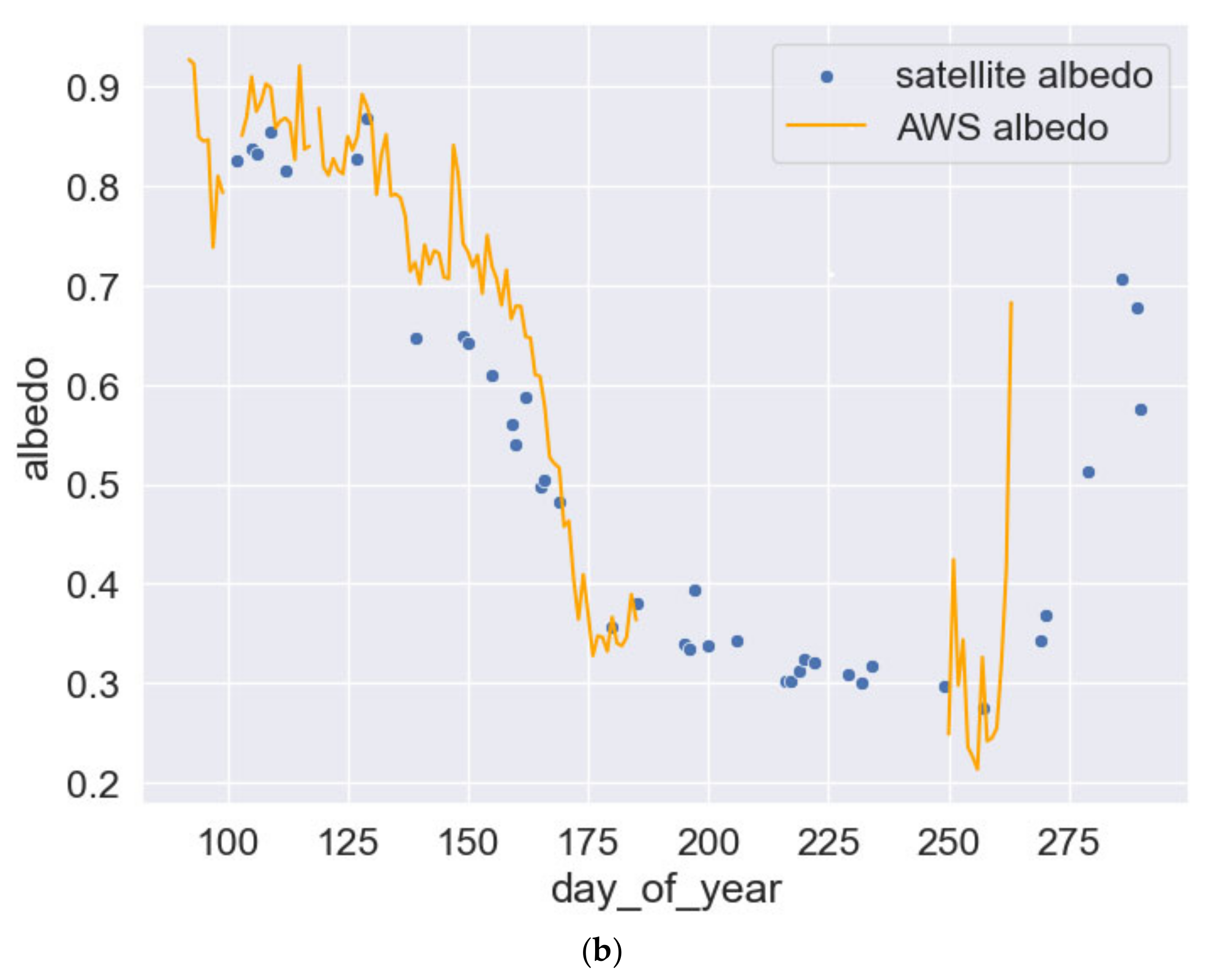
Figure 1. The geometry of the problem.
Remotesensing 18 02929 g001
Figure 2. (a) The EnMAP true color browse images of the area. (b) The illustration of the performance of the pixel identification algorithm (0-water, 1-bare land, 2-glacier ice and snow surfaces, 3-clouds, see color bar). (c) MSI (S-2) browse image of the studied area.
Remotesensing 18 02929 g002aRemotesensing 18 02929 g002b
Figure 3. The glacier height (a) and derived slope (b) spatial distributions.
Remotesensing 18 02929 g003
Figure 4. The spectral measured and retrieved TOA and BOA reflectances and BOA plane albedo over snow (upper curves) and bare ice (lower set of curves) for two selected EnMAP ground pixels (snow-covered and bare ice ground scene with lower reflection). The calculations have been performed using Equation (33) for TOAR, Equation (6) for BOAR, and Equation (7) for plane albedo.
Remotesensing 18 02929 g004
Figure 5. EnMAP reflectances at channels 424 (a) and 1048 nm (b) over snow and glacier ice.
Remotesensing 18 02929 g005aRemotesensing 18 02929 g005b
Figure 6. The retrieved spatial distribution and frequency of black sky EnMAP BBA.
Remotesensing 18 02929 g006
Figure 7. The spatial distribution of EnMAP NRMSD (in percent) (a) and its frequency (b).
Remotesensing 18 02929 g007aRemotesensing 18 02929 g007b
Figure 8. The spatial distribution of the error of retrievals without accounting for the surface slope (a) and its frequency distribution (b).
Remotesensing 18 02929 g008aRemotesensing 18 02929 g008b
Figure 9. The intercomparison of shortwave black sky BBA spatially collocated retrievals using EnMAP and two S2 algorithms (a,b)—algorithm 1: HLS, (c,d)—algorithm 2: ICEHLS).
Remotesensing 18 02929 g009aRemotesensing 18 02929 g009b
Figure 10. The intercomparison of shortwave black sky BBA spatially collocated retrievals using Landsat (a,b), MODIS (c,d), and EnMAP data.
Remotesensing 18 02929 g010aRemotesensing 18 02929 g010b
Figure 11. The intercomparison of shortwave black sky BBA spatially collocated retrievals using OLCI and EnMAP data ((a)—correlation plot, (b)—frequency distribution of BBA).
Remotesensing 18 02929 g011
Figure 12. The latitudinal dependence of BBA derived using EnMAP and other instruments. The vertical spread of data for the same instrument is due to slight dependence of the BBA on the longitude. The dependence of BBA on the latitude (especially in the ice-snow transition zone) is more pronounced.
Remotesensing 18 02929 g012
Figure 13. The same as in Figure 11, except the OLCI BBA results have been derived using the EnMAP retrieval algorithm.
Remotesensing 18 02929 g013
Figure 14. The spectral measured and retrieved TOA and BOA reflectances and BOA plane albedo over snow (upper set of curves) and bare ice (lower set of curves) for two selected OLCI ground pixels (snow-covered and bare ice ground scene with lower reflection). The calculations have been performed using Equation (33) for TOAR, Equation (6) for BOAR, and Equation (7) for plane albedo.
Remotesensing 18 02929 g014
Figure 15. (a) The TAS_L PROMICE station. The photo is taken on 6 September 2025 (courtesy B. Vandecrux). One can see that a cloud system approaches the station. (b) The photo is taken on 6 September 2025, several kilometers from the TAS_L PROMICE station. One can see the network of ice/melting water channels on the surface of the glacier. (c) The example of the surface texture at the station.
Remotesensing 18 02929 g015aRemotesensing 18 02929 g015b
Figure 16. The temporal behavior of temperature and albedo at the ground PROMICE TAS_L station (a). The satellite albedo is derived using ESA S-2 satellite measurements in the framework of the ICEHLS algorithm discussed above (b).
Remotesensing 18 02929 g016aRemotesensing 18 02929 g016b
Table 1. Various definitions of the black sky broadband albedo depending on the spectral integration limits λ 1 ,   λ 2 . The visible broadband albedo also includes the part of the UV range (350–400 nm).
BBAShortwave
(SW)
Visible
(VIS)
Near-Infrared (NIR)
NotationA A V I S A N I R
λ 1 , nm 350350700
λ 2 , nm 25007002500
Table 2. The atmospheric radiative transfer characteristics used in the retrieval process. The spectral functions R a t m ( λ ) , T a t m ( λ ) , and r a t m ( λ ) are determined under the assumption that gaseous absorption in the atmosphere is absent.
Radiative Transfer CharacteristicNotion
TOA reflectance for black underlying surface R a t m ( λ )
Two-way TOA transmittance for black underlying surface T a t m ( λ )
Atmospheric spherical albedo for black underlying surface r a t m ( λ )
Two-way gaseous TOA transmittance for black underlying surface T g a s ( λ )
Table 3. Thresholds for the pixel identification procedure. The thresholds are applied in the order given in the table. In the case of clouds, all thresholds must be satisfied simultaneously.
Underlying SurfaceThresholdsIndex
WaterR (1026 nm) < 0.060
Bare landR (418 nm) < 0.351
CloudsR (1379 nm)/R (2120 nm) < 0.03
R (418 nm) > 0.35, R (1235 nm)/R (418 nm)   0.3
3
Bare glacier ice and snowIf all criteria above are not met2
Table 4. The values of the correlation coefficient R, the RMSD, linear regression (y = ax + b) coefficients, and the sample size (N) as derived using EnMAP and multiple satellite observations.
InstrumentRRMSDabN
Landsat0.97270.05550.91960.08722594
MSI/S2, algorithm 10.97430.05580.90320.10034193
MSI/S2, algorithm 20.93720.05980.76720.11073598
OLCI/S30.92710.09510.61810.21141834
MODIS0.96100.06981.00260.04051137
Table 5. The difference between BBA derived from various retrieval techniques and instruments for the selected snow and glacier ice areas.
InstrumentBBA (Snow)BBA (Glacier Ice)Bias/Relative Bias (Snow)Bias/Relative Bias (Glacier Ice)
EnMAP0.74030.3447--
SGLI0.7553-0.0150/2.0%-
OLCI0.67710.4506−0.0642/−9.5%0.1059/+23.5%
MODIS0.78460.30600.0443/5.6%−0.0387/−12.65%
Landsat-0.38840.0437/11.3%0.0437/11.25
S-2/algorithm 10.78760.4085+0.0473/6.0%0.0638/15.6%
S-2/algorithm 20.66530.4251−0.0750/−11.3%0.0804/18.9
Table 6. The intercomparison with ground measurements (the value of ground measurements was 0.28 at noon on 6 September 2025).
InstrumentBlack Sky BBADifference
(Satellite–Ground)
Spatial
Resolution, m
Time of
Measurements
EnMAP0.299+0.019/7%3014:51
Landsat0.265−0.015/−5%3013:54
MSI/S2, algorithm 10.265−0.015/−5%3014:14
MSI/S2, algorithm 20.294+0.014/+5%3014:14
OLCI/S30.309+0.029/10%50013:32
MODIS/
TERRA
0.244−0.036/13%50016 days
Disclaimer/Publisher’s Note: The statements, opinions and data contained in all publications are solely those of the individual author(s) and contributor(s) and not of MDPI and/or the editor(s). MDPI and/or the editor(s) disclaim responsibility for any injury to people or property resulting from any ideas, methods, instructions or products referred to in the content.



