Machine-Learning-Based Radar Quantitative Precipitation Estimation Using Intra-Hour Temporal Features from Dual-Polarization Observations

Highlights

What are the main findings?

• Intra-hour temporal features derived from ten consecutive 6 min dual-polarization radar observations provide additional information for hourly QPE beyond instantaneous radar intensity.
• Feature importance diagnostics show that dominant predictors shift from ZH-related descriptors at 0–5 mm h⁻¹ to KDP-derived descriptors in higher rainfall intensity classes.

What are the implications of the main findings?

• ML-based radar QPE should incorporate physically meaningful representations of intra-hour polarimetric evolution, rather than relying mainly on algorithm selection.
• Rainfall-imbalance-aware evaluation is necessary because natural rainfall distributions may mask systematic errors in heavy rainfall estimation.

Abstract

Hourly precipitation is a standard variable for hydrological applications, flood warning, and quantitative assessment of precipitation-related hazards. Weather radar provides high-frequency observations, but these sub-hourly measurements must be linked to hourly rain-gauge accumulations for radar-based quantitative precipitation estimation (QPE). This study develops a machine-learning-based hourly radar QPE framework using intra-hour temporal features from dual-polarization observations. Each hourly gauge accumulation was matched with ten consecutive 6 min radar observations. Six temporal features were derived from dual-polarization observations, including the mean, sum, standard deviation, linear trend, maximum, and skewness. The results show clear rainfall regime dependence in the contribution of polarimetric variables. Evaluation of machine-learning models confirms the value of intra-hour temporal features, with the best-performing model achieving an RMSE of 3.96 mm h⁻¹, compared with 6.42 mm h⁻¹ for the linear baseline. The experiments further show that the complete temporal feature set improves QPE performance. Diagnostic evaluation also indicates that model bias is sensitive to the representation of heavy rainfall samples. These findings suggest that ML-based radar QPE should emphasize physically meaningful intra-hour polarimetric features and rainfall-imbalance-aware sampling.

1. Introduction

Accurate quantitative precipitation estimation (QPE) is fundamental to hydrologic applications and flood early warning, especially for warm-season convective precipitation, which is highly intermittent and spatially heterogeneous [1,2]. Weather radar provides high-temporal- and high-spatial-resolution observations and has therefore become a cornerstone of real-time precipitation monitoring. Compared with conventional single-polarization radar, dual-polarization systems offer improved microphysical characterization through polarimetric variables, including horizontal reflectivity (ZH), differential reflectivity (ZDR), and specific differential phase (KDP). These measurements can improve QPE accuracy and robustness under calibration uncertainty, signal attenuation, and natural variability in raindrop size distributions [3,4,5,6].

Despite these advantages, radar-based QPE still faces considerable challenges. Conventional parametric relations, including ZH–R, KDP–R, and hybrid polarimetric formulations, are highly sensitive to precipitation regime, melting-layer contamination, and regional variability [7,8]. As a result, their coefficients are often non-stationary, limiting transferability and generalizability. In addition, operational implementations frequently rely on single-scan estimates or simple temporal aggregation, which may inadequately represent sub-hourly storm evolution [9,10]. This limitation becomes particularly evident when 6 min radar observations are related to hourly gauge accumulations, because reducing within-hour variability to a single aggregated value can obscure storm growth, decay, and structural evolution that are relevant to hourly rainfall totals [11].

Machine-learning (ML) approaches provide a promising alternative by learning nonlinear relationships between multidimensional radar predictors and surface rainfall without prescribing fixed microphysical assumptions. Recent studies have shown that ML methods can exploit interactions among ZH, ZDR, and KDP and thereby improve QPE performance [12,13,14]. Nevertheless, several aspects merit further investigation. First, the temporal mismatch between sub-hourly radar sampling and hourly gauge accumulation is often handled implicitly, rather than through explicit representation of intra-hour evolution [15,16]. Second, a systematic comparison across different ML algorithm families remains valuable for robust model selection and uncertainty assessment in radar-based QPE [17]. Third, the contribution of dual-polarization variables to ML-based QPE is still rarely interpreted in a rainfall-regime-dependent manner, particularly with respect to how the relative importance of ZH, ZDR, and KDP changes with rainfall intensity [18]. In addition, the scarcity of heavy-rain samples may bias models toward light-rain regimes, leading to the underestimation of intense precipitation.

In this study, we develop and evaluate an hourly QPE framework that improves rainfall estimation by explicitly incorporating intra-hour radar evolution. A large radar–gauge matched dataset over eastern China during the summers of 2021 and 2022 is used, in which each hourly gauge accumulation is paired with a sequence of consecutive 6 min dual-polarization radar mosaics. From these sequences, we derive hourly predictors from ZH, ZDR, and KDP, so that each hourly sample contains information on radar intensity, variability, and temporal evolution within the accumulation period. Eight representative regression algorithms from different ML families are then systematically compared. Their performance is evaluated using graphical diagnostics and quantitative metrics, and the contribution of dual-polarization variables is examined through feature importance analysis for the full sample and for different rainfall intensity classes. This study investigates whether incorporating intra-hour radar evolution can enhance hourly QPE, how different ML algorithm families respond to such evolution-aware predictors, and how the contribution of polarimetric variables varies across rainfall intensity regimes.

The remaining parts of this paper are organized as follows. In Section 2, the dataset, quality control, radar–gauges matching and feature construction are described. The performance of the eight QPE algorithms and the dependence on dual-polarization predictors across rainfall regimes are analyzed in Section 3. In Section 4, the implications and limitations are discussed, and the conclusions are summarized in Section 5.

2. Data and Methods

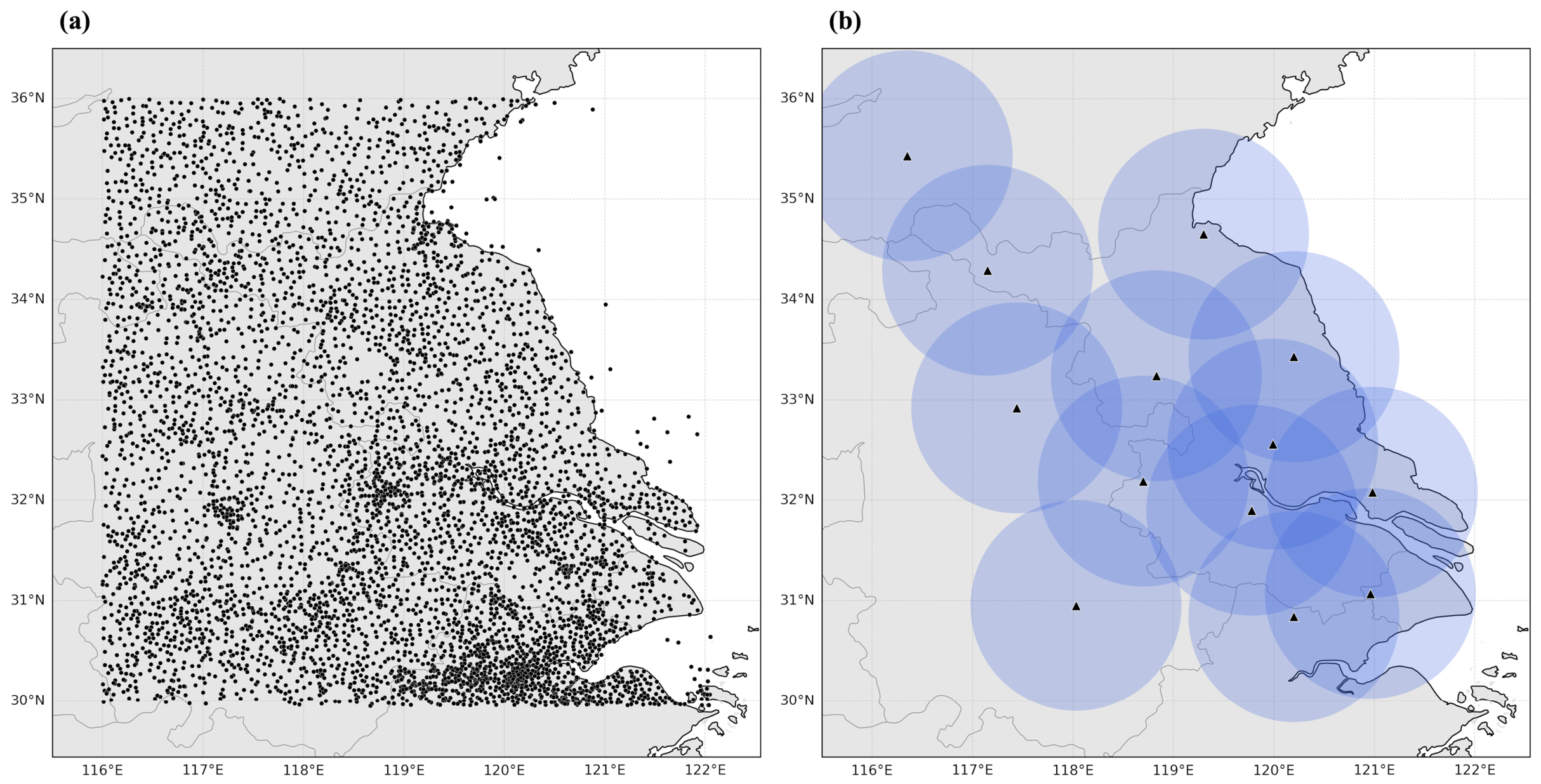
The dataset used in this study comprised S-band dual-polarization radar mosaic products and surface rain-gauge measurements over eastern China during the warm seasons of 2021 and 2022, specifically from June to August in each year (Figure 1). The regional radar mosaics were generated from volume scan data collected by 13 S-band dual-polarization weather radars at 6 min intervals. All radars used the same operational volume coverage pattern, with each volume scan consisting of nine elevation angles: 0.5°, 1.5°, 2.4°, 3.4°, 4.3°, 6.0°, 9.9°, 14.6° and 19.5°. The operational maximum scanning range was 230 km. In this study, however, only quality-controlled radar observations within 110 km of the radar sites were used for radar–gauge matching and QPE model development, in order to reduce range-related uncertainties associated with beam broadening, beam overshooting, and vertical representativeness at longer ranges. This volume scanning strategy is consistent with the operational scanning configuration of the China New Generation Weather Radar network, which has been described in previous studies [19]. Non-meteorological echoes, including ground clutter, anomalous propagation, and other spurious signals, were identified and removed using a logic-based fuzzy-logic classification algorithm [20]. After quality control, the polar-coordinate radar observations were interpolated onto a Cartesian grid with a horizontal resolution of 0.01° to generate three-dimensional regional radar mosaics. The machine-learning QPE framework used these quality-controlled gridded radar mosaics, rather than raw polar-coordinate volume scans from individual radars, as the radar input data. Specifically, ZH, ZDR, and KDP were extracted from the 3 km constant-altitude mosaic level for radar–gauge matching and QPE model development.

Hourly accumulated precipitation observations from 5489 operational surface rain gauges were used as reference measurements. The gauge observations had undergone routine operational quality control through the Meteorological Data Operation System (MDOS) of the China Meteorological Administration. Each gauge was paired with the radar mosaic grid point covering the gauge location, forming 5489 fixed rain-gauge–radar grid point pairs. These pairs were repeatedly matched in time with hourly gauge accumulations and ten consecutive 6 min radar mosaics to generate the hourly sample set. Samples with missing gauge precipitation, negative or physically invalid precipitation values, or missing radar mosaic variables at the corresponding gauge location were excluded before model training and evaluation.

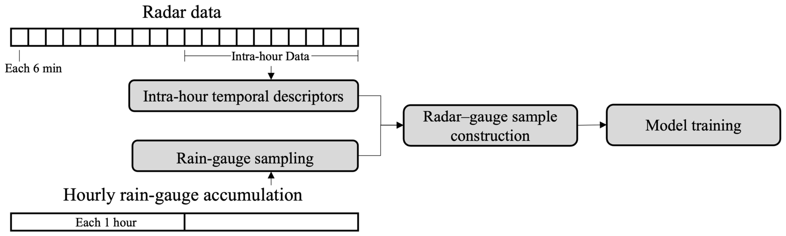
For each hourly rain-gauge accumulation ending at time t, ten consecutive 6 min radar mosaics at the 3 km constant-altitude level within the corresponding accumulation period were extracted, namely at t-54 min, t-48 min, …, and t min (Figure 2). At each radar time step, ZH, ZDR and KDP at the gauge location were sampled from the quality-controlled 3 km gridded mosaics using nearest-neighbor interpolation. The resulting 10-step radar mosaic sequence was then converted into an 18-dimensional feature vector by calculating six intra-hour temporal descriptors for each of the three polarimetric variables. The corresponding hourly gauge precipitation was used as the supervised learning target. Therefore, each machine-learning sample followed a sequence-to-scalar structure, in which the intra-hour radar evolution was encoded as radar-derived predictors and paired with one hourly gauge precipitation value.

To compactly represent intra-hour storm evolution, time-series features were derived from the 10-frame radar sequence for each polarimetric variable (

Table 1. Definitions of the six intra-hour temporal descriptors for each polarimetric radar variable, ZH, ZDR, and KDP. 

Feature	Statistical Interpretation	Definition
mean	Mean state within the hourly accumulation period	$\overline{X}={\displaystyle \frac{1}{N}}{\displaystyle \sum _{i=1}^N}X,N=10$
sum	Within-hour temporal aggregation in the native radar measurement space	$X_{\mathrm{sum}}={\displaystyle \sum _{i=1}^N}{X}_i$
std	Intra-hour variability	$X_{\mathrm{std}}=\sqrt{{\displaystyle \frac{1}{N-1}}{\displaystyle \sum _{i=1}^N}{\left(X_i-\overline{X}\right)}^2}$
slope	Linear temporal tendency	$\mathrm{Slope}\mathrm{coefficient}\mathrm{from}\mathrm{a}\mathrm{least}\text{-}\mathrm{squares}\mathrm{linear}\mathrm{fit}\mathrm{of}{X}_i$$\mathrm{against}\mathrm{the}\mathrm{scan}\mathrm{index}i$.
Max	Maximum intensity	$X_{\max }=\max \{X_i{\}}_{i=1}^N$
skew	Asymmetry of distribution	$X_{\mathrm{skew}}={\displaystyle \frac{1}{N}}{\sum }_{i=1}^N{\left({\displaystyle \frac{X_i-\overline{X}}{\sigma }}\right)}^3,\sigma$ is the sample standard deviation

Note: X denotes one of the three polarimetric radar variables, ZH, ZDR, or KDP. Each descriptor was calculated separately for the three variables; therefore, the complete predictor set contains 18 variables for each sample.

). Specifically, six statistical descriptors, including the mean, sum, standard deviation, linear trend, maximum, and skewness, were calculated for each of ZH, ZDR, and KDP, yielding 18 predictors for each radar–gauge matched sample. These features were designed to characterize the intensity level, within-hour temporal aggregation, temporal fluctuation, evolutionary tendency, peak state, and distributional asymmetry of polarimetric signatures within the hourly accumulation period. The descriptors were calculated in the native units of the operational radar mosaic products, namely dBZ for ZH, dB for ZDR, and deg km⁻¹ for KDP. For logarithmic variables such as ZH and ZDR, these descriptors should be interpreted as statistical summaries in the radar measurement space, rather than as linear physical accumulations.

Eight representative regression algorithms from different model families were evaluated for hourly quantitative precipitation estimation (QPE), including Ridge regression, k-nearest neighbors (KNN), multilayer perceptron (MLP), random forest (RF), Extremely Randomized Trees (ExtraTrees), Gradient Boosting Decision Trees (GBDTs), Histogram-based Gradient Boosting Decision Trees (HGBDTs), and XGBoost. These algorithms were selected to represent linear, instance-based, neural-network, bagging-ensemble, and boosting-ensemble modeling frameworks. For the scale-sensitive models, namely Ridge, KNN, and MLP, the predictor variables were standardized to zero mean and unit variance using StandardScaler embedded in a scikit-learn pipeline (version 1.5.1). The scaler was fitted only on the training data and then applied to the test data, thereby ensuring consistent preprocessing and avoiding data leakage.

Model training, hyperparameter tuning, and performance evaluation were implemented in Python (3.12.7) using the scikit-learn and XGBoost libraries (version 2.1.4) [21,22]. The radar–gauge matched samples were randomly divided into training and test subsets, with 70% of the samples used for model training and hyperparameter tuning and the remaining 30% retained for independent testing. All preprocessing steps, including feature standardization for scale-sensitive models, were fitted only on the training subset and then applied to the test subset to avoid data leakage. Hyperparameters were optimized using grid search with cross-validation on the training subset, and fixed random seeds were used where applicable to improve reproducibility. Model performance was evaluated using mean absolute error (MAE), root mean square error (RMSE), and the coefficient of determination (R²), together with scatterplot-based diagnostic analysis.

Three traditional radar QPE baselines, namely ZH–R, KDP–R, and ZH–ZDR–R, were implemented for comparison with the machine-learning models (

Table 2. Calibrated coefficients of the traditional radar QPE baselines. 

Baseline QPE	Form	Calibrated Relation
ZH–R	$R=a{Z}_H^b$	$R=0.5025Z_H^{0.3200}$
KDP–R	$R=a{\left(K_{DP}^{*}\right)}^b$	$R=11.8511{\left(K_{DP}^{*}\right)}^{0.3914}$
ZH–ZDR–R	$\ln \left(R\right)={\mathsf{\beta }}_0+{\mathsf{\beta }}_1\ln \left(Z_H\right)+{\mathsf{\beta }}_{2}ZDR$	$R=0.5044Z_H^{0.3193}\exp \left(0.004745ZDR\right)$

Note: R denotes scan-level rain rate in mm h⁻¹. Where ZH is in dBZ. $K_{DP}^{\mathrm{*}}=\max \left(K_{DP},0.01\right)$. ZDR is in dB. For each hourly sample, the calibrated relation was first applied separately to the ten 6 min radar scans within the hourly accumulation period. The resulting scan-level rain rate estimates were then converted to 6 min rainfall amounts and summed to obtain the hourly radar-based precipitation estimate. All coefficients were calibrated using only the 2021–2022 training subset.

). For these traditional baselines, the empirical relations were first applied separately to each of the ten 6 min radar scans within the hourly accumulation period to obtain scan-level rain rate estimates. The resulting scan-level rain rates were then converted to 6 min rainfall amounts and summed to match the corresponding hourly gauge precipitation. ZH was converted from dBZ to linear reflectivity before fitting. The ZH–R and KDP–R baselines were expressed as power-law relations, $R=a{\mathit{ZH}}^b$ and $R=aKD{P}^b$, respectively, while the ZH–ZDR–R baseline was expressed as $\ln \left(R\right)={\mathsf{\beta }}_0+{\mathsf{\beta }}_1\ln \left(Z_H\right)+{\mathsf{\beta }}_{2}ZDR$. The coefficients of these relations were calibrated only on the 2021–2022 training subset and then directly evaluated on the independent June 2024 dataset. The June 2024 data were not used for coefficient fitting or model tuning.

Rainy samples were defined as hourly gauge precipitation ≥ 1.0 mm h⁻¹ and stratified into six rainfall intensity classes: 1–5, 5–10, 10–25, 25–50, 50–100, and ≥100 mm h⁻¹. A stratified random split was then performed with a fixed random seed of 42, assigning 70% of the samples to model training and hyperparameter tuning and 30% to the holdout test set. The eight-model intercomparison used the complete 70% training set and was evaluated primarily on the complete 30% holdout test set. To diagnose model behavior under a less long-tailed rainfall distribution, a capped rainfall-intensity-balanced diagnostic subset was constructed from the independent holdout test set and used only for evaluation; up to 6000 samples were retained from each rainfall class without replacement, with smaller classes retained in full, resulting in 24,656 samples using a fixed random seed of 1042. A separate capped balanced training subset was constructed from the 70% training set only for the MLP training distribution sensitivity experiment, not for the main eight-model comparison; up to 12,000 samples were retained from each rainfall class without replacement, resulting in 49,531 samples using a fixed random seed of 542. Detailed sample counts for each subset are provided in Table S2.

3. Results

3.1. Analysis of Dual-Polarization Radar Dependence

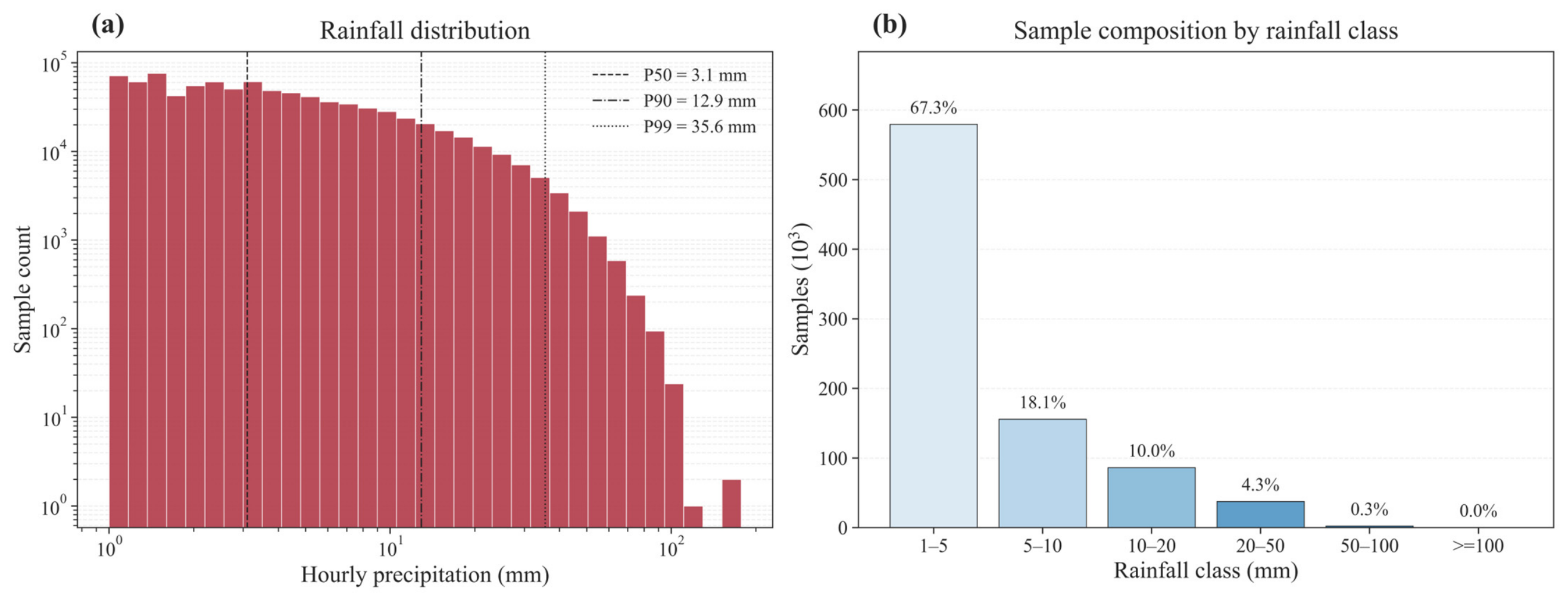
Figure 3 shows the distribution of hourly gauge precipitation. The rainfall samples exhibit a pronounced right-skewed structure, with frequency decreasing rapidly as precipitation intensity increases (Figure 3a). The median, 90th percentile, and 99th percentile are 3.1, 12.9, and 35.6 mm h⁻¹, respectively. The class-wise composition further highlights this imbalance (Figure 3b). Specifically, 67.3% of the samples fall within the 1–5 mm h⁻¹ class, 18.1% within 5–10 mm h⁻¹, and 10.0% within 10–20 mm h⁻¹, while only 4.3% exceed 20 mm h⁻¹. This distribution demonstrates a clear long-tail structure, indicating that model training is mainly constrained by the abundant lower-intensity samples, whereas the statistical support for rainfall above 20 mm h⁻¹ is much more limited.

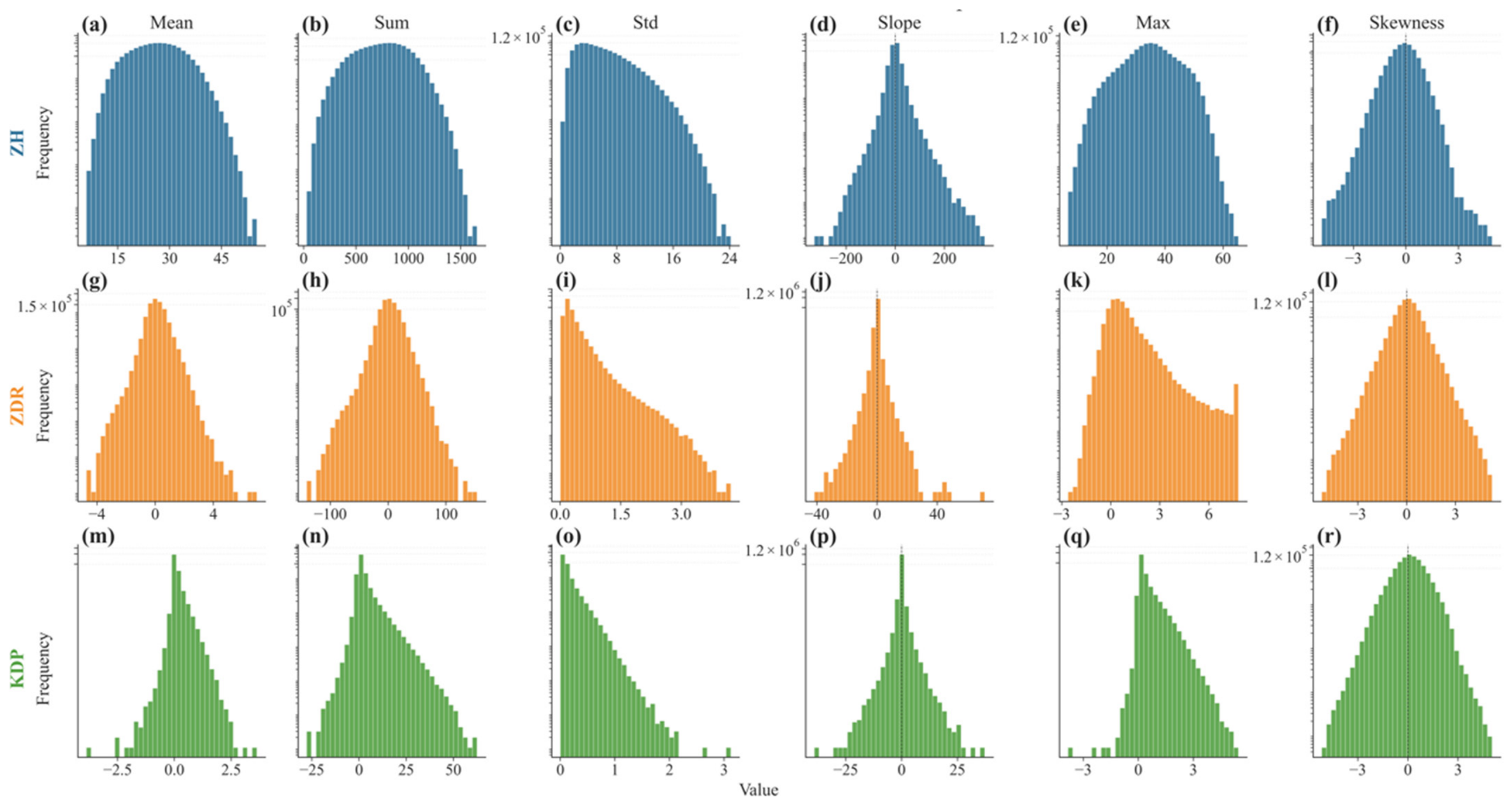
Figure 4 presents the distributions of the intra-hour radar-derived features for ZH, ZDR, and KDP. For ZH, the mean, sum, standard deviation, and maximum are mainly concentrated within low-to-moderate ranges, indicating that most samples are associated with weak-to-moderate echo intensity. The slope distribution is sharply centered near zero, suggesting that persistent intensification or weakening within the hourly accumulation period occurs only in a limited subset of samples. In contrast, the features derived from ZDR and KDP exhibit broader and less regular distributions, particularly for the sum, standard deviation, maximum, and skewness. Some KDP-derived descriptors show a considerable number of negative or near-zero values. This behavior is mainly associated with weak-rainfall samples, for which the true KDP is close to zero and the phase-derived KDP estimate is more susceptible to residual ΦDP noise, smoothing-window effects, and local nonuniform beam filling. Therefore, small negative KDP values should be interpreted as retrieval uncertainty around zero rather than physically negative rainfall intensity. Because light rainfall dominates the matched dataset, such values are frequently reflected in the KDP_mean and KDP_sum distributions. These values were retained after quality control rather than being artificially truncated to zero, in order to avoid distorting the weak-rainfall KDP distribution. This behavior suggests that these polarimetric variables are more sensitive to variations in raindrop shape, liquid-water content, and the internal structural evolution of precipitation systems. Moreover, the relatively broad spreads of standard deviation, slope, and skewness across the three variables indicate substantial diversity in sub-hourly radar evolution among different samples.

These distributional characteristics have direct implications for the QPE problem addressed in this study. On the one hand, the strong imbalance of rainfall samples suggests that accurate estimation of high-intensity precipitation is intrinsically more difficult than that of light rainfall, because heavy-rain samples provide much weaker statistical support for model training and evaluation. On the other hand, the radar predictors exhibit marked heterogeneity not only in magnitude but also in temporal variability and asymmetry, indicating that hourly precipitation cannot be adequately represented by instantaneous radar intensity alone, particularly when sub-hourly radar observations are matched to hourly gauge accumulations [15,16]. Instead, the within-hour evolution of polarimetric signatures may contain additional information relevant to rainfall estimation. These characteristics provide a physical and statistical basis for incorporating multi-feature radar representations into the machine-learning framework and for subsequently examining model performance across different rainfall regimes.

3.2. Feature Importance of Dual-Polarization Radar Predictors

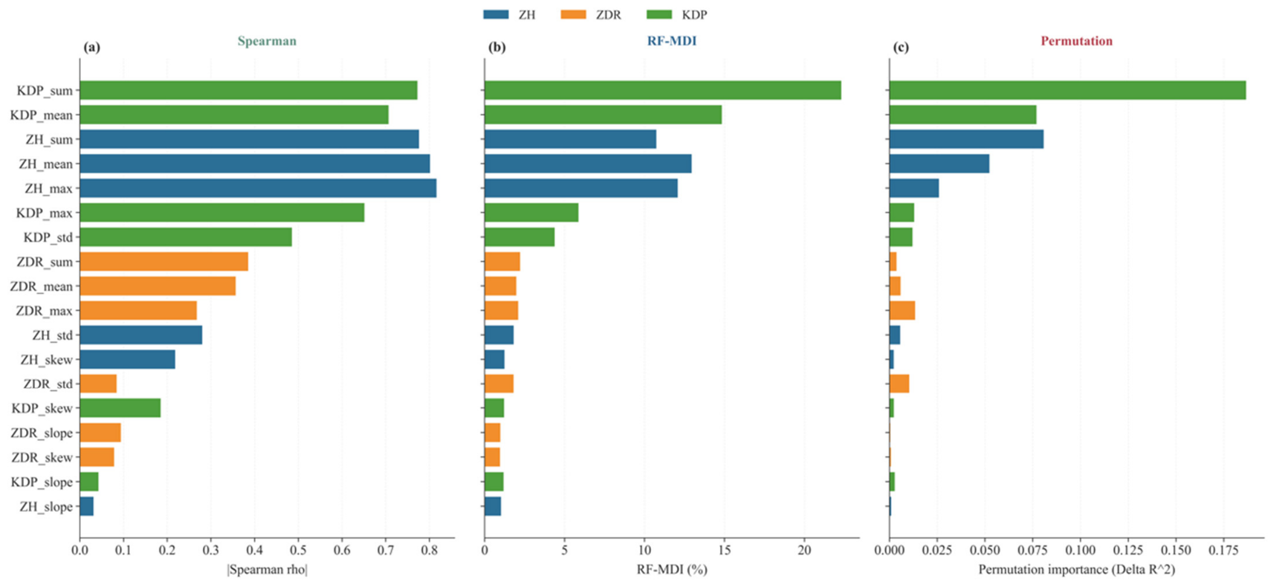
To provide a more reliable assessment of predictor relevance in hourly QPE, feature importance was analyzed using a multi-diagnostic framework that combined absolute Spearman rank correlation, random forest mean decrease in impurity (RF-MDI), and test set permutation importance. These diagnostics quantify predictor relevance from different angles, including marginal monotonic association with rainfall, contribution to the RF decision structure, and actual performance degradation after feature perturbation. Using these complementary measures reduces reliance on any single ranking criterion and provides a more robust interpretation of predictor importance. In total, 2,712,451 quality-controlled radar–gauge matched samples were retained for this analysis. Because the number of samples decreased sharply with increasing rainfall intensity, especially for extreme rainfall, the rain-rate-stratified importance analysis was limited to bins below 100 mm h⁻¹; the ≥100 mm h⁻¹ bin contained only 15 samples and was therefore excluded to avoid unstable estimates.

At the full-sample level, the importance ranking is consistently dominated by KDP- and ZH-related predictors, whereas ZDR-derived features play a secondary but non-negligible role (Figure 5). Across all three metrics, KDP_sum emerges as the most influential predictor, or one of the most influential predictors, while KDP_mean, ZH_sum, ZH_mean, and ZH_max also rank prominently. This overall pattern indicates that hourly precipitation is jointly constrained by reflectivity magnitude and phase-based accumulation. The strong contribution of ZH-related predictors reflects the first-order dependence of rainfall on echo intensity, whereas the prominence of KDP-derived predictors highlights the added value of differential phase information, which is closely related to liquid-water content, raindrop concentration, and intense rain-bearing regions [23,24]. By contrast, ZDR-derived variables contribute less strongly at the full-sample level, suggesting that differential reflectivity is not the primary predictor of hourly rainfall amount, but rather a complementary descriptor of raindrop shape, size sorting, and microphysical variability.

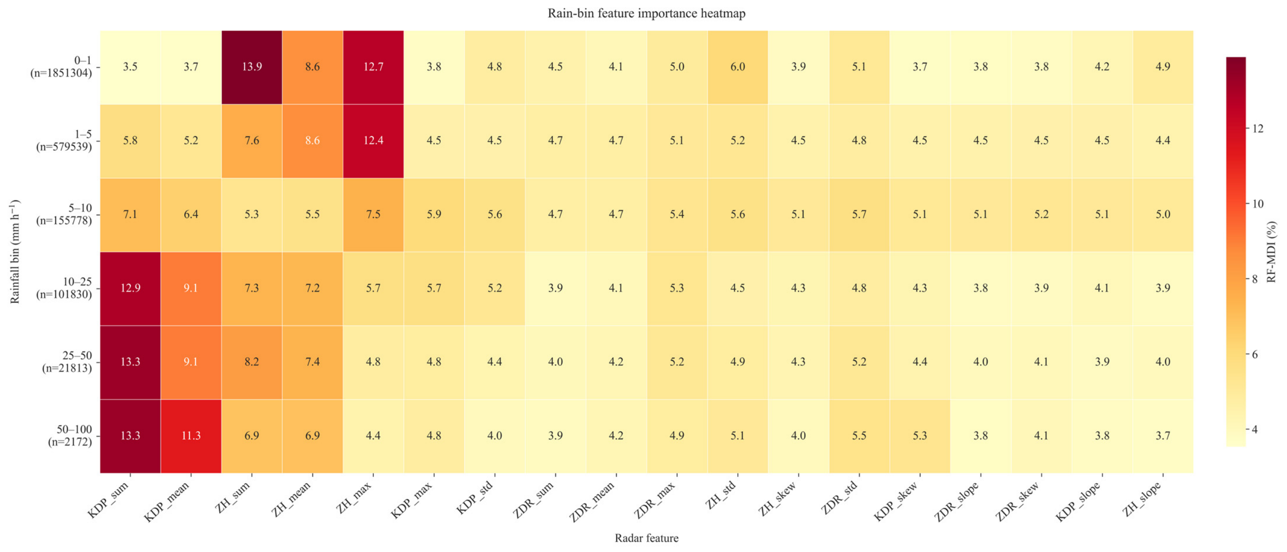
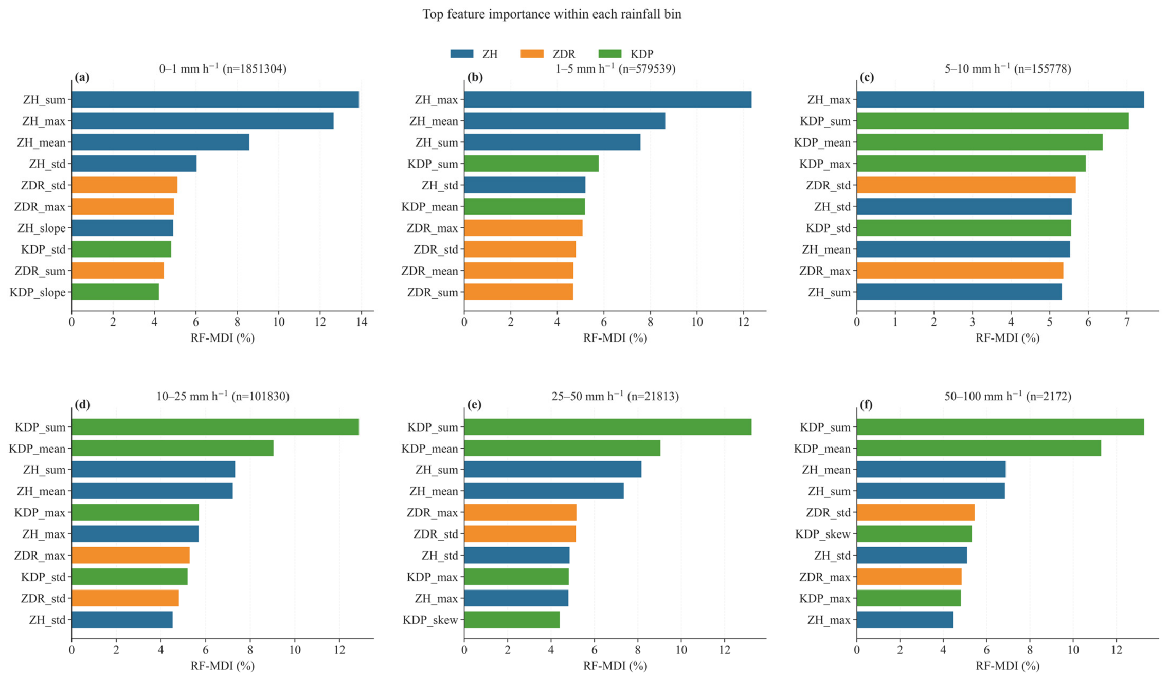
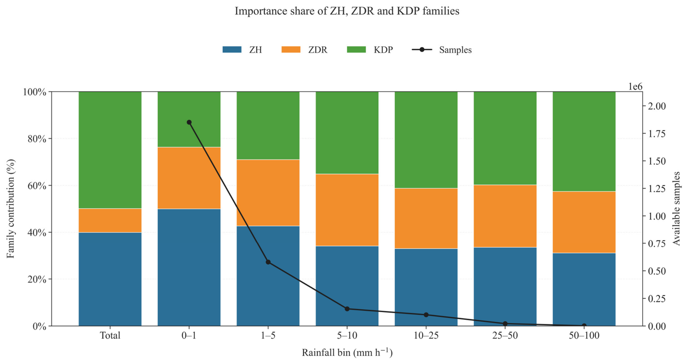
Although the overall ranking is informative, it partly masks the strong heterogeneity of predictor importance across rainfall regimes. This regime dependence becomes evident when the RF-MDI analysis is repeated separately for each rainfall bin (Figure 6, Figure 7 and Figure 8). In the 0–1 and 1–5 mm h⁻¹ classes, the leading predictors are dominated by ZH-based descriptors such as ZH_sum, ZH_max, and ZH_mean. Correspondingly, the family-level contribution of ZH reaches about 50.0% in the 0–1 mm h⁻¹ bin and remains as high as 42.7% in the 1–5 mm h⁻¹ bin (Figure 8). This result indicates that, under weak-rainfall conditions, hourly accumulation is primarily constrained by the bulk magnitude of reflectivity. Physically, this behavior is expected because KDP is typically small in light rain and is therefore more susceptible to noise, while ZDR carries less direct rainfall information when hydrometeor populations are relatively small and microphysical contrast remains limited.

As rainfall intensity increases, the dominant information source gradually shifts from reflectivity-based predictors toward phase-based predictors. In the 5–10 mm h⁻¹ class, KDP-derived features become comparable to the leading ZH predictors, and in the 10–25, 25–50, and 50–100 mm h⁻¹ classes, KDP_sum becomes the highest-ranked feature, with KDP_mean also remaining among the top contributors (Figure 6 and Figure 7). At the family level, the contribution of KDP rises to about 41.2%, 39.8%, and 42.6% in the 10–25, 25–50, and 50–100 mm h⁻¹ bins, respectively (Figure 8), clearly exceeding its contribution in the light-rain regime. This transition from ZH-dominated importance in the 0–1 and 1–5 mm h⁻¹ classes to KDP-enhanced or KDP-dominated importance in the 10–25, 25–50, and 50–100 mm h⁻¹ classes is physically meaningful. Under stronger precipitation, KDP becomes more robust and more sensitive to rainwater content, while reflectivity-based estimates are more easily affected by nonlinearity, calibration uncertainty, and saturation-like behavior at high echo intensity. The results therefore suggest that the controlling radar information for hourly QPE is not fixed, but varies systematically with rainfall regime.

A supplementary diagnostic analysis was added to assess predictor collinearity and robust group-level importance (Figure S1). The Spearman correlation matrix shows substantial collinearity among several predictors, especially between mean and sum descriptors derived from the same radar variable. The maximum absolute Spearman correlation reached 0.991, indicating that individual feature rankings should be interpreted with caution. Group permutation and ablation tests show that KDP-related predictors provide the largest radar variable family contribution, while temporal aggregation, maximum, and mean descriptors dominate at the descriptor level. The smaller ablation losses relative to group permutation effects indicate that correlated predictors can partially compensate for one another after model retraining, supporting the interpretation of feature importance at the group rather than single-variable level.

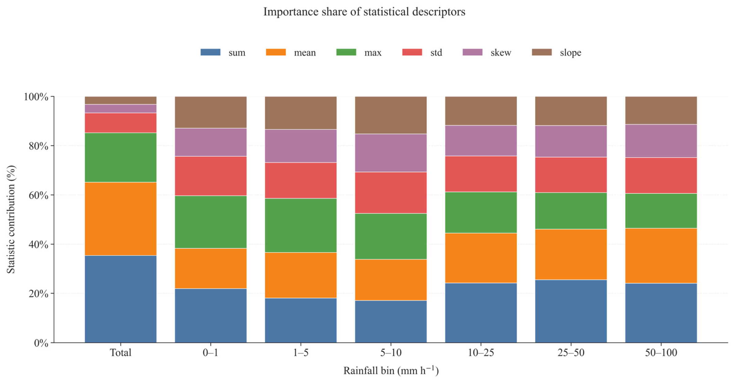
A similar rainfall intensity dependence is also evident when predictors are grouped by statistical descriptor rather than by radar variable family (Figure 9). At the full-sample level, sum, mean, and max are the three dominant descriptor types, contributing about 35.3%, 29.8%, and 20.1%, respectively. This indicates that hourly QPE depends primarily on within-hour temporal aggregation of radar signatures, average state, and peak intensity within the hour. However, the relative importance of these descriptor types also changes with rainfall intensity. In the 0–1 and 1–5 mm h⁻¹ classes, max and sum are both prominent, implying that short-lived reflectivity peaks and the persistence of radar signatures within the hour are both relevant for distinguishing lower hourly rainfall amounts. In contrast, in the 10–25 and 25–50 mm h⁻¹ classes, the contribution of sum and mean becomes more pronounced, suggesting that sustained radar signatures and their temporally aggregated descriptors provide more useful information than isolated peaks for estimating larger hourly totals. Descriptors representing temporal variability and temporal structure, including std, skew, and slope, do not dominate the ranking, but their contributions remain stable across most bins. This indicates that within-hour variability does not replace the mean or temporally aggregated signal level as the primary constraint on hourly rainfall, but provides complementary information for distinguishing rainfall processes with similar overall intensity but different temporal organization.

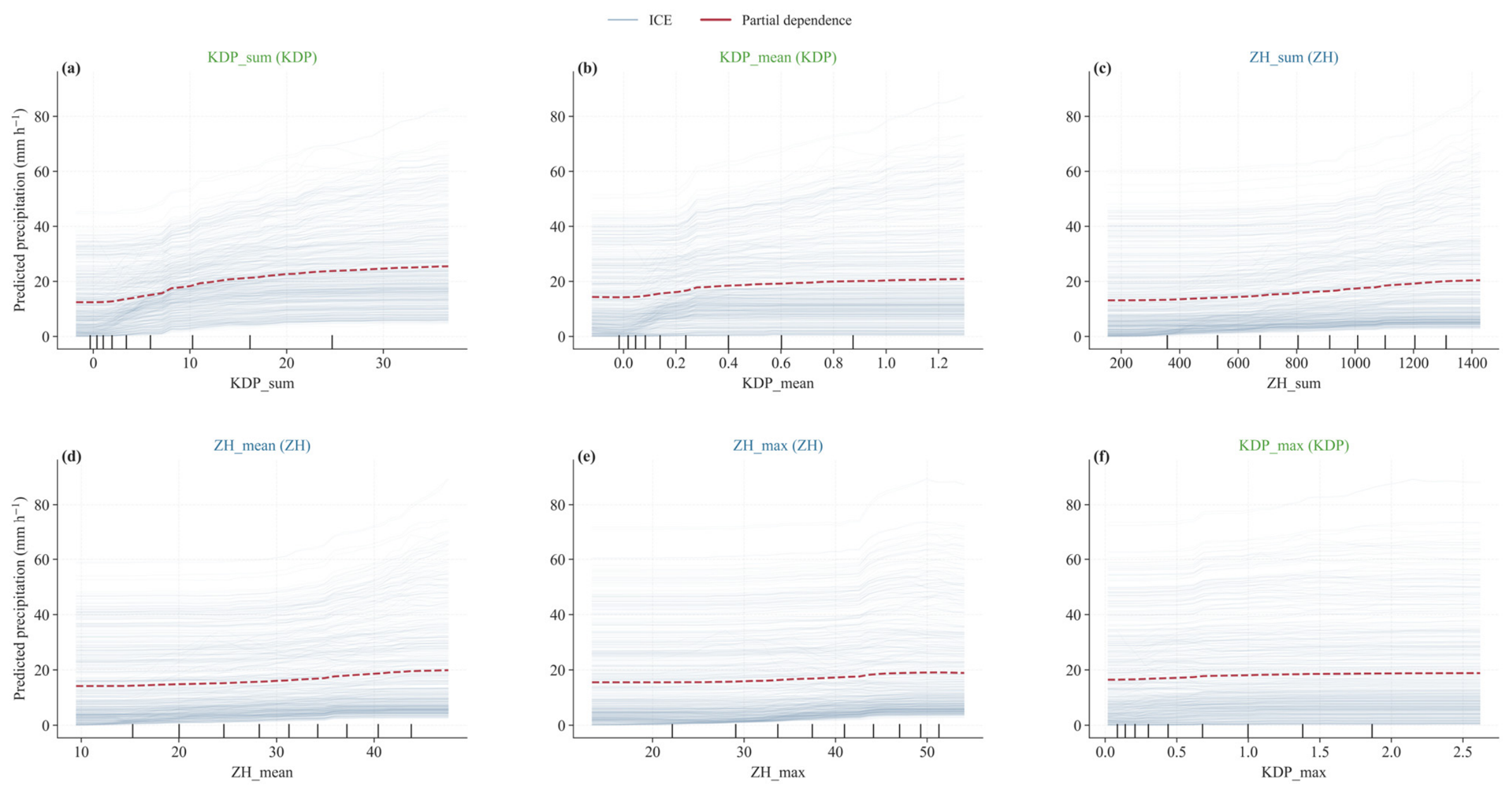
The partial dependence plot (PDP) and individual conditional expectation (ICE) diagnostics of the most influential predictors provide further support for the regime-dependent interpretation of radar information (Figure 10). The PDP curves describe the average marginal response of the model to a given predictor, whereas the ICE curves display the corresponding response for individual samples. The average PDP curves for KDP_sum, KDP_mean, ZH_sum, ZH_mean, ZH_max, and KDP_max all show positive but distinctly nonlinear relationships with RF-predicted hourly rainfall. Instead of following a single linear response, these curves exhibit segmented increases and varying slopes across the predictor range. For KDP_sum and KDP_mean, predicted rainfall increases rapidly after low-value thresholds and continues to increase at higher values, indicating that temporally aggregated and mean phase-based descriptors provide increasingly strong constraints as rainfall intensity increases. The ZH-based predictors also show generally increasing responses, but their slopes become flatter in some higher-value ranges, suggesting that the marginal gain in predictive information is not uniform across the full reflectivity range. The broad spread of the ICE curves indicates substantial sample-to-sample heterogeneity in predictor responses, implying that the influence of an individual radar feature depends on the surrounding multivariate context rather than acting independently.

Collectively, these analyses indicate a clear regime-dependent use of dual-polarization radar information in the ML-based hourly QPE framework. For light rainfall, the model primarily relies on reflectivity-related features, suggesting that the bulk magnitude of ZH provides the main constraint on weak hourly accumulations. As rainfall intensity increases, KDP-derived temporal aggregation and mean descriptors become increasingly prominent and eventually dominate in the 10–25, 25–50, and 50–100 mm h⁻¹ classes, consistent with the enhanced sensitivity of phase-based information to liquid-water content and intense rain-bearing regions. ZDR-derived features contribute across rainfall classes, but mainly as complementary microphysical indicators related to drop shape and size variability rather than as primary controls on rainfall amount. From the perspective of temporal feature types, sum, mean, and maximum features consistently outweigh variability-oriented features such as standard deviation, skewness, and slope, indicating that hourly QPE is primarily governed by within-hour temporal aggregation, mean state, and peak intensity within the accumulation period, while sub-hourly variability provides additional discrimination. The PDP and ICE analyses further suggest that these relationships cannot be fully represented by simple linear or single-power-law formulations. Overall, the results support the use of machine-learning models that can flexibly integrate nonlinear, multivariate, and rainfall-regime-dependent information from dual-polarization radar observations for hourly precipitation estimation.

3.3. Comparison of Machine-Learning QPE Algorithms

To assess the influence of regression framework selection on hourly radar-based QPE, all valid rainy samples were divided into training and testing subsets using a stratified 70/30 holdout strategy. The stratification was performed according to rainfall intensity classes, so that the primary holdout test set retained the natural long-tailed rainfall distribution while providing an independent evaluation of model generalization. Eight representative regression models were compared, covering linear regression, instance-based learning, neural networks, bagging ensembles, and boosting ensembles: Ridge, KNN, MLP, RF, ExtraTrees, GBDT, HGBDT, and XGBoost (Table S1). Because rainfall samples are highly imbalanced and heavy rainfall cases are rare but hydrologically important, an additional rainfall intensity-stratified diagnostic subset was constructed from the independent holdout set. This subset was used only for evaluation, not for model training, and was designed to reduce the dominance of light-rain samples in the performance statistics. Therefore, the natural 30% holdout set was used to quantify overall predictive performance under the observed sample distribution, whereas the diagnostic subset was used to examine the sensitivity of model errors and systematic bias to rainfall intensity sampling.

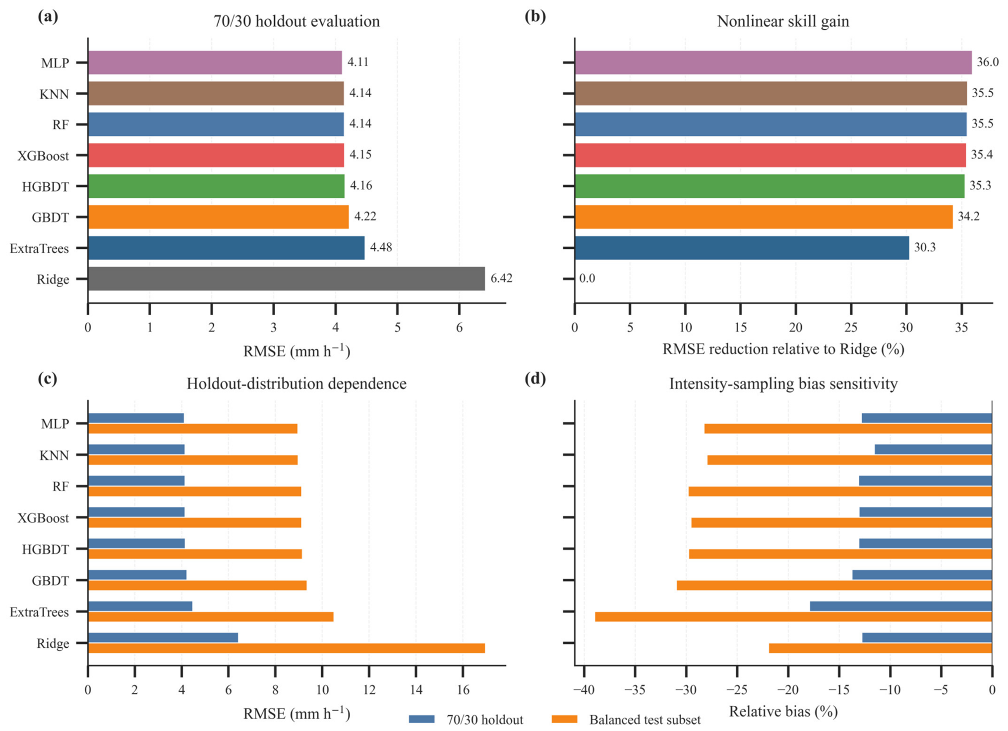
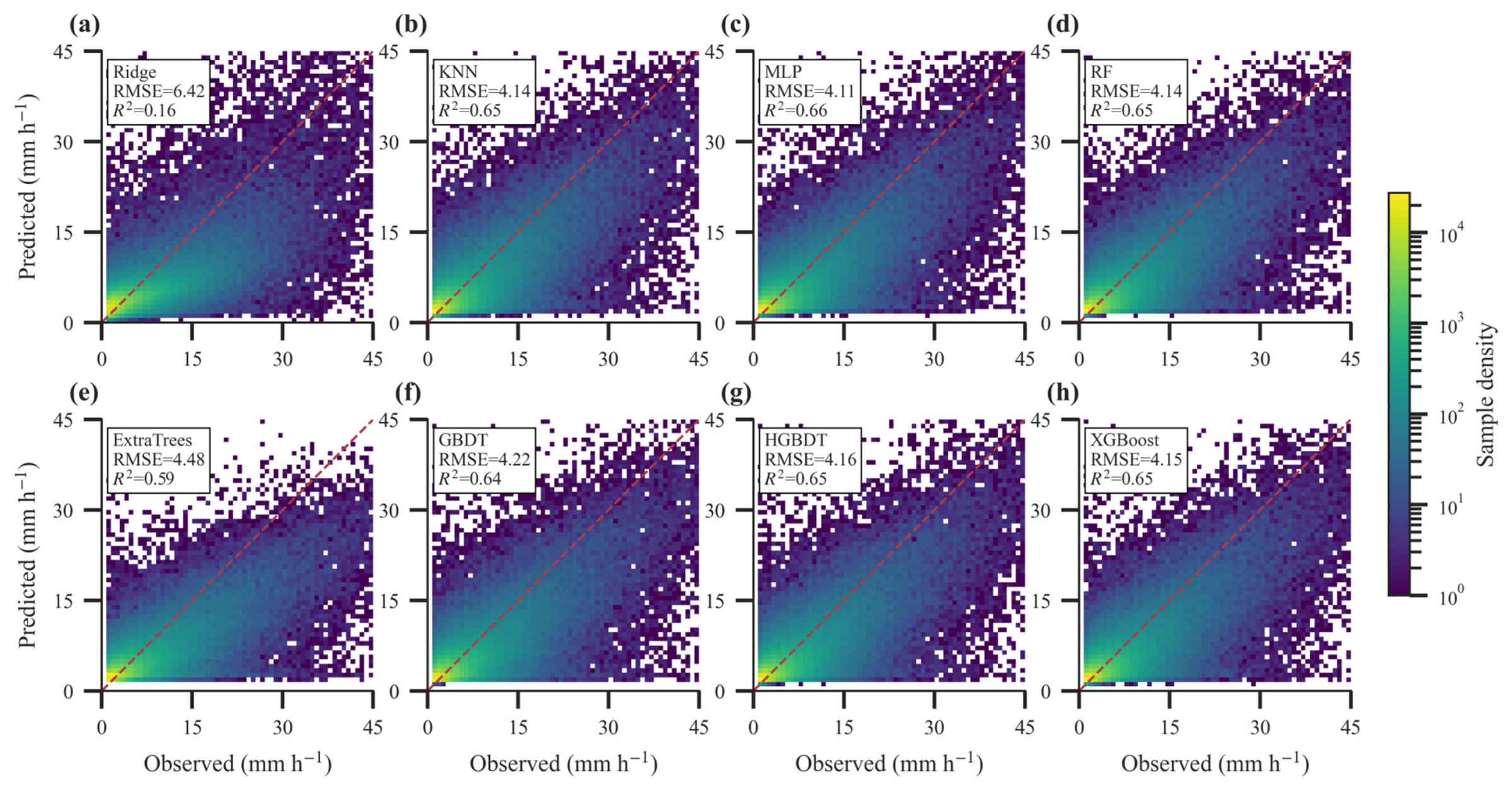
The overall evaluation shows a clear advantage of nonlinear models over the linear Ridge baseline (Figure 11a,b). Ridge yields the largest RMSE of 6.42 mm h⁻¹, whereas the nonlinear models reduce RMSE to 4.11–4.48 mm h⁻¹, corresponding to a reduction of approximately 30–36% relative to Ridge. MLP achieves the lowest RMSE, 4.11 mm h⁻¹, followed closely by KNN, RF, XGBoost, and HGBDT, whose RMSE values differ only slightly. This indicates that the primary improvement arises from the ability of nonlinear models to represent threshold-like responses and interactions among intra-hour dual-polarization features, rather than from the unique superiority of a single algorithm. The relatively small differences among the leading nonlinear models further suggest that the constructed radar features can be effectively exploited by multiple model families.

Model evaluation is also strongly affected by the rainfall intensity composition of the test samples (Figure 11c,d). All models exhibit larger RMSE on the rainfall-intensity-balanced diagnostic subset than on the natural 70/30 holdout subset, because the diagnostic subset increases the relative contribution of samples in the higher rainfall intensity classes. More importantly, the relative bias comparison reveals clear intensity sampling sensitivity. Although all models show negative relative bias under both test protocols, the bias becomes substantially more negative when the test subset is balanced by rainfall intensity. For example, the relative bias of MLP changes from 12.83% on the natural holdout subset to 28.27% on the balanced diagnostic subset, while that of XGBoost changes from 13.07% to 29.53%. This indicates that the apparent overall bias estimated from the natural holdout subset is partly moderated by the dominance of samples below 10 mm h⁻¹, for which the models tend to show near-zero or slight positive bias. When the contribution of moderate and heavy rainfall samples is increased, the systematic underestimation of larger rainfall amounts becomes much more evident. Therefore, model bias should not be interpreted as a fixed global quantity, but as a distribution-dependent diagnostic that is strongly influenced by the rainfall intensity composition of the evaluation set.

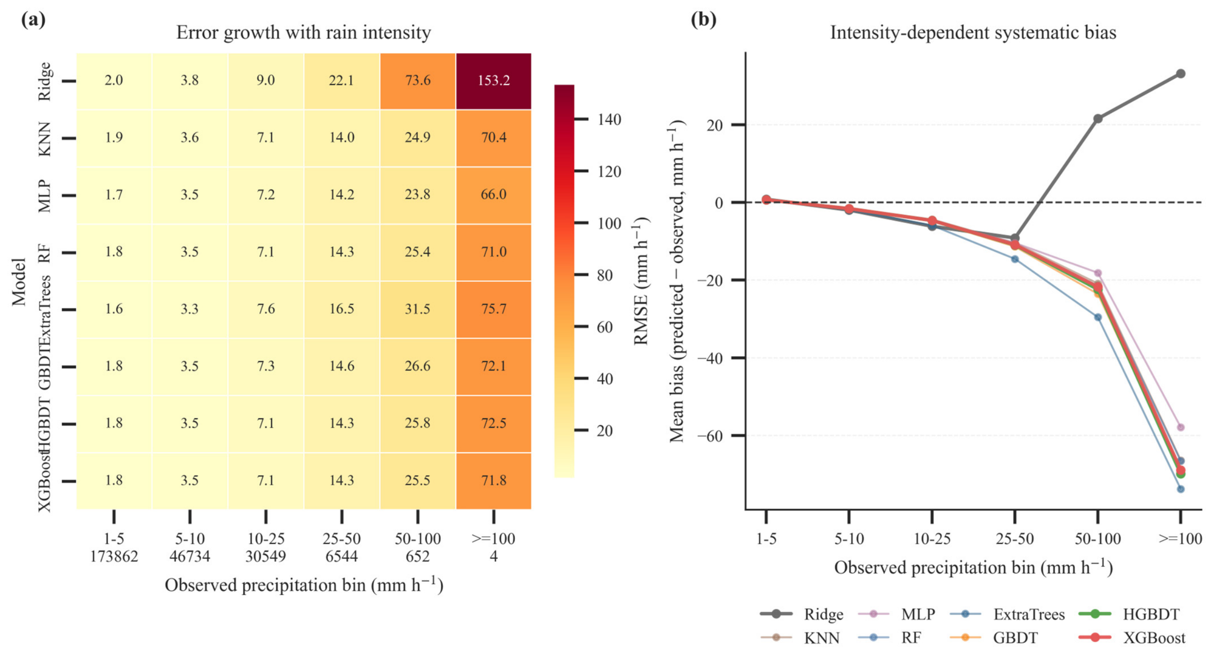
The rainfall-stratified diagnostics and observed–predicted density distributions jointly reveal the intensity-dependent structure of QPE errors (Figure 12 and Figure 13). For the nonlinear models, RMSE remains low in the 1–5 and 5–10 mm h⁻¹ bins, increases to approximately 7–8 mm h⁻¹ in the 10–25 mm bin, rises to about 14–17 mm h⁻¹ in the 25–50 mm h⁻¹ bin, and further increases to approximately 24–32 mm h⁻¹ in the 50–100 mm h⁻¹ bin. The bias curves show a consistent transition from near-zero or slight positive bias in the 1–5 and 5–10 mm h⁻¹ classes to increasingly negative bias in the 25–50 and 50–100 mm h⁻¹ classes, which explains the stronger negative relative bias observed on the rainfall-intensity-balanced diagnostic subset. The density scatterplots support this interpretation: compared with the pronounced prediction compression of Ridge, the nonlinear models produce more concentrated distributions along the 1:1 reference line, particularly for low-to-moderate rainfall. The irregular Ridge bias above 50 mm h⁻¹ is attributable to prediction compression toward the dominant low-to-moderate rainfall range and the limited statistical support of upper-tail samples, rather than to numerical non-convergence. However, upper-tail samples remain frequently below the 1:1 line, indicating persistent underestimation of high observed rainfall. Because only four samples are available in the >100 mm h⁻¹ bin, the corresponding statistics should be interpreted only qualitatively. These results show that the evaluated skill of ML-based QPE algorithms is strongly affected by the representation of heavy rainfall samples. When high-intensity rainfall is rare in the test set, overall metrics are dominated by weaker rainfall and may mask substantial errors in the upper tail.

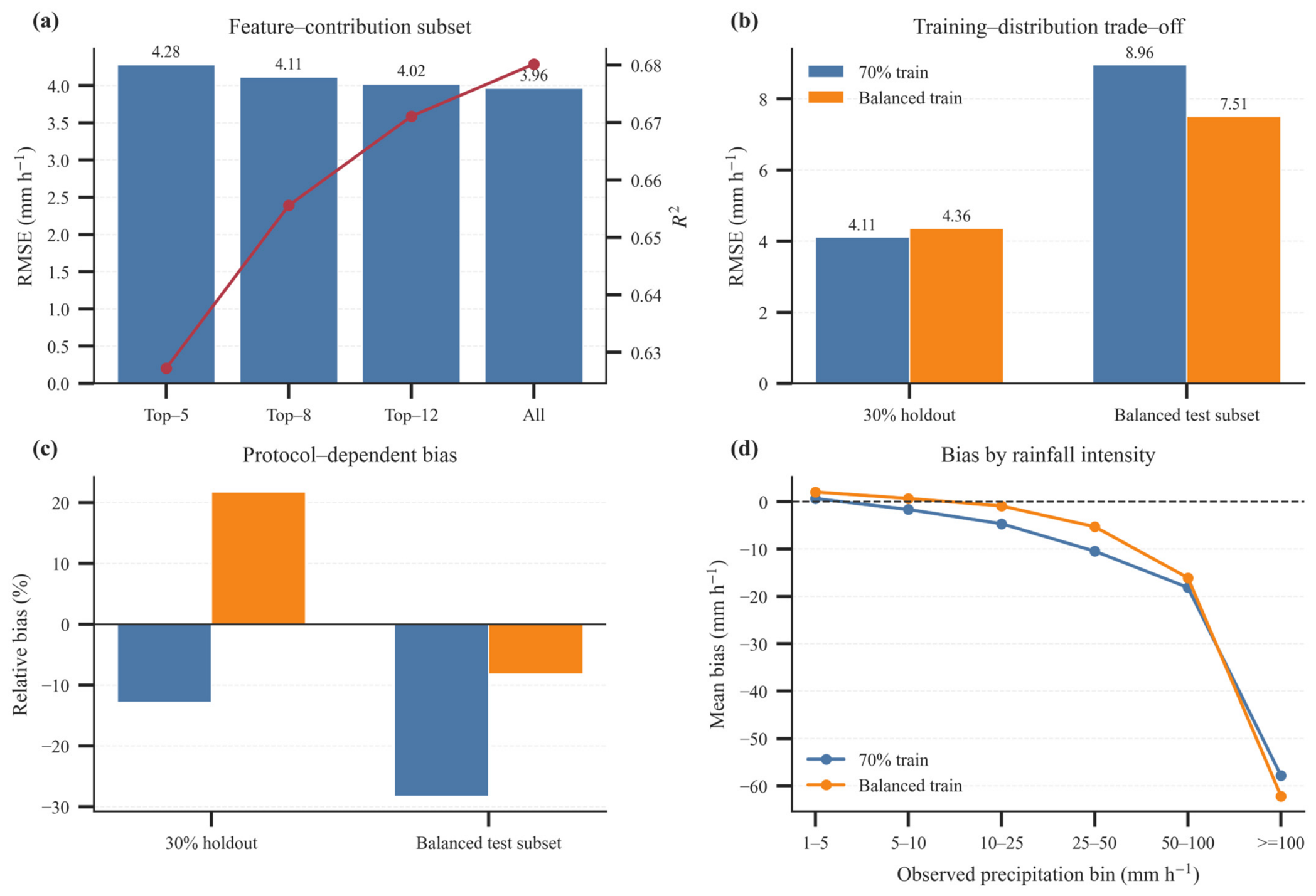
To assess the effect of feature subset size, the predictors were ranked according to their feature importance scores, and four input configurations were compared: the Top-5, Top-8, Top-12, and all 18 radar-derived features. The sensitivity experiments further demonstrate that model behavior is controlled by both feature completeness and rainfall sample distribution (Figure 14). For MLP, RMSE decreases from 4.28 mm h⁻¹ using the Top-5 predictors to 3.96 mm h⁻¹ using all 18 predictors, while R² increases from 0.627 to 0.680, indicating that lower-ranked temporal and distributional features provide useful incremental information. This suggests that hourly QPE benefits from a more complete representation of intra-hour radar evolution, rather than relying only on the most dominant predictors. Modifying the training distribution introduces a trade-off: balanced training slightly worsens performance on the natural holdout subset, with RMSE increasing from 4.11 to 4.36 mm h⁻¹, but improves performance on the rainfall-intensity-balanced diagnostic subset, reducing RMSE from 8.96 to 7.51 mm h⁻¹ and weakening the negative bias in moderate-to-heavy rainfall bins. These results indicate that the evaluated skill and bias of ML-based QPE models are shaped not only by the representation of heavy rainfall samples, but also by how effectively intra-hour polarimetric evolution is encoded. Therefore, ML-based radar QPE should increasingly emphasize physically informed representations of intra-hour polarimetric evolution and rainfall-imbalance-aware sampling strategies, rather than relying mainly on the selection of a particular machine-learning algorithm.

3.4. Independent Temporal Validation

To further evaluate the transferability of the proposed framework to unseen rainfall events, an independent temporal validation was conducted using all valid rainy samples from June 2024. The June 2024 dataset was completely excluded from model training, hyperparameter tuning, feature ranking, and coefficient calibration. The machine-learning models trained using the 2021–2022 radar–gauge dataset were directly applied to the June 2024 samples. To compare the proposed framework with established radar QPE baselines, three traditional radar–rainfall relations, including ZH–R, KDP–R, and ZH–ZDR–R, were also implemented. Their coefficients were calibrated only using the 2021–2022 training subset and then evaluated on the independent 2024 dataset.

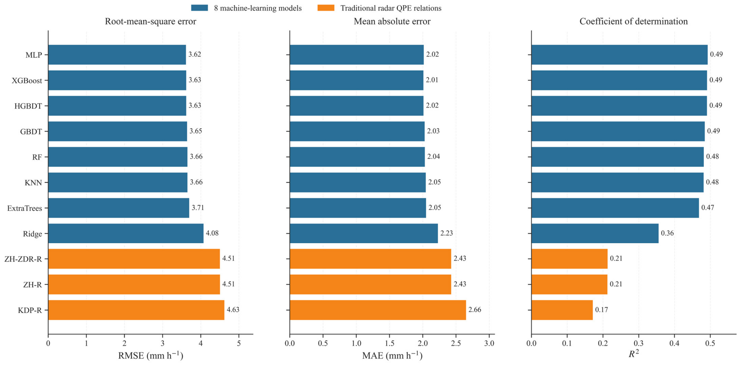
The independent validation confirms that the machine-learning models retain their advantage on unseen rainfall samples (Figure 15). The leading ML models achieve RMSE values of 3.62–3.66 mm h⁻¹, MAE values of 2.01–2.05 mm h⁻¹, and R² values of 0.48–0.49. In comparison, the traditional radar QPE relations yield higher RMSE values of 4.51–4.63 mm h⁻¹ and lower R² values of 0.17–0.21. Among the ML models, MLP achieves the lowest RMSE, while XGBoost and HGBDT show nearly identical performance. These results indicate that the improvement of the proposed temporal feature-based framework is not limited to the original 70/30 holdout experiment, but remains evident when applied to an independent month from a different year.

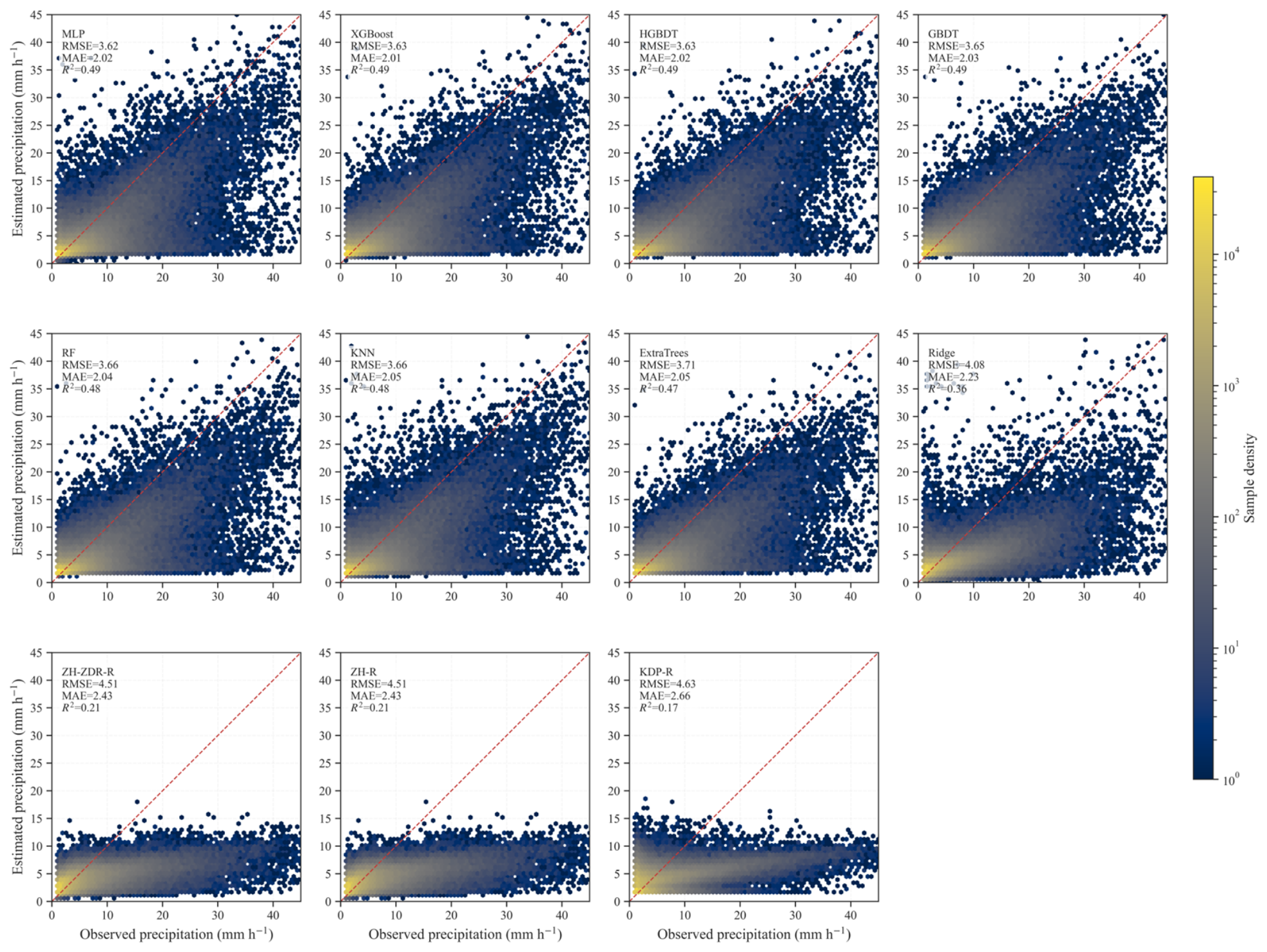
The density scatterplots further reveal differences in the error structure between the ML models and traditional radar QPE relations (Figure 16). The ML estimates show a more continuous distribution around the 1:1 reference line, whereas the traditional relations exhibit stronger prediction compression, particularly for higher observed rainfall intensities. This pattern indicates that the intra-hour temporal descriptors help the ML models better represent nonlinear radar–rainfall relationships than fixed-form empirical relations. Nevertheless, high-intensity rainfall samples remain more dispersed and are still frequently underestimated, suggesting that upper-tail rainfall estimation remains a key challenge even under independent temporal validation.

4. Discussion

This study highlights the importance of explicitly representing intra-hour polarimetric evolution for hourly radar QPE. Previous studies have emphasized that radar–rainfall estimation and radar–gauge comparison are strongly affected by spatiotemporal representativeness, sampling scale, and observation uncertainty, particularly in hydrological and urban applications that require short-duration rainfall information [9,25,26]. Recent radar–gauge merging studies have also shown the value of combining radar spatial information with gauge-based accumulation constraints for high-resolution rainfall estimation [27,28]. In this context, the proposed intra-hour temporal features provide a compact bridge between 6 min dual-polarization radar observations and hourly gauge accumulations by summarizing the mean state, within-hour temporal aggregation, peak intensity, temporal variability, trend, and distributional asymmetry of ZH, ZDR, and KDP. The feature subset experiment further shows that using the full set of intra-hour predictors improves model skill relative to using only the highest-ranked features, indicating that lower-ranked temporal and distributional features still provide complementary information through nonlinear interactions. This suggests that ML-based hourly QPE should emphasize intra-hour polarimetric feature representation, rather than relying solely on instantaneous radar intensity or a few dominant predictors.

The feature importance analysis further reveals that the value of dual-polarization information is rainfall-regime-dependent. In the 0–1 and 1–5 mm h⁻¹ classes, ZH-related features dominate, indicating that reflectivity magnitude provides the primary constraint on lower hourly accumulations. With increasing rainfall intensity, KDP-derived cumulative and mean descriptors become increasingly important, especially in the 10–25, 25–50, and 50–100 mm h⁻¹ classes, consistent with the stronger sensitivity of phase-based variables to liquid-water content and intense rain-bearing regions. This agrees with classical and recent polarimetric QPE studies showing that KDP and other phase-based measurements provide information beyond reflectivity and are particularly useful for constraining moderate-to-heavy rainfall [23,24,29,30]. This is consistent with disdrometer-based and polarimetric studies emphasizing the microphysical relevance of ZDR, particularly its association with raindrop shape, raindrop size distribution variability, and hydrometeor sorting [29,31]. These results extend previous ML-based radar QPE studies, which demonstrated the ability of machine-learning models to learn nonlinear relationships from operational or large radar–gauge datasets [13,14], by showing that the relative contribution of ZH, ZDR, and KDP is not fixed but changes systematically with rainfall intensity.

The algorithm comparison and sampling experiments further show that ML-based radar QPE is strongly affected by the representation of heavy rainfall samples. Although all nonlinear models outperform the Ridge baseline, the leading algorithms show comparable performance, suggesting that the main gain arises from nonlinear representation rather than from a specific model choice, consistent with previous ML-based QPE studies [13,32]. More importantly, model skill and bias vary substantially with the rainfall intensity composition of the test samples. The natural holdout subset is dominated by samples below 10 mm h⁻¹, whereas the rainfall-intensity-balanced diagnostic subset gives greater weight to the 25–50 and 50–100 mm h⁻¹ classes and therefore exposes stronger negative bias at higher rainfall intensities. This intensity-dependent error structure is consistent with previous radar QPE studies reporting larger uncertainties and underestimation at high rainfall intensities [9,29]. The balanced training experiment further indicates that increasing the representation of moderate and heavy rainfall can reduce negative bias in the diagnostic subset, but may slightly reduce average performance under the natural rainfall distribution. These results suggest that ML-based radar QPE should place greater emphasis on heavy rainfall-aware sampling and evaluation, together with physically meaningful representations of intra-hour polarimetric evolution.

Although no explicit convective–stratiform classification was performed, the rainfall-intensity-stratified diagnostics provide insight into convective-rainfall-relevant conditions because warm-season convective rainfall is typically associated with higher hourly rainfall intensity. The leading nonlinear models show broadly comparable behavior in the 25–50 and 50–100 mm h⁻¹ classes, whereas Ridge exhibits stronger prediction compression; nevertheless, all models show increased error and negative bias in these upper rainfall intensity classes, indicating that intense rainfall remains a common limitation.

In addition to radar-related uncertainties, gauge-related uncertainty should also be noted. Although the gauge observations used in this study had undergone routine operational quality control and were used as the reference measurements for model training and evaluation, they should not be interpreted as error-free rainfall truth. Gauge-based precipitation estimates may still be affected by wind-induced undercatch, intensity-dependent errors of tipping-bucket gauges during intense rainfall, missing-data screening uncertainty, and the representativeness mismatch between point-scale gauges and 0.01° radar mosaic grid cells. These uncertainties may influence both model training and independent evaluation, particularly for localized high-intensity rainfall. Therefore, the QPE performance reported in this study should be interpreted as performance relative to gauge-referenced hourly precipitation. Future work should evaluate the proposed framework across different regions, seasons, and independent rainfall events, particularly for high-intensity rainfall classes where sample availability remains limited.

5. Conclusions

To improve hourly radar quantitative precipitation estimation, this study developed a machine-learning-based framework using intra-hour temporal features derived from dual-polarization radar observations. Ten consecutive 6 min radar observations were matched with each hourly rain-gauge accumulation, and six temporal features were extracted from ZH, ZDR, and KDP. The main conclusions are as follows:

(1) The intra-hour temporal features provide useful information for hourly QPE beyond instantaneous radar intensity. Using all 18 temporal features outperformed the Top-5, Top-8, and Top-12 feature subsets, indicating that lower-ranked temporal and distributional features still contribute additional information through nonlinear interactions.

(2) The contribution of dual-polarization variables is clearly rainfall-intensity-dependent. ZH-related descriptors dominate the 0–1 and 1–5 mm h⁻¹ classes, whereas KDP-derived descriptors, especially KDP_sum and KDP_mean, become leading predictors in the 10–25, 25–50, and 50–100 mm h⁻¹ classes. This shift indicates that ML-based hourly QPE relies increasingly on phase-based information as rainfall intensity increases, while ZDR-derived descriptors provide complementary microphysical information.

(3) Nonlinear machine-learning models substantially improve QPE performance compared with the Ridge baseline. However, the differences among the leading nonlinear models are relatively small, suggesting that the main gain comes from nonlinear representation of radar–rainfall relationships rather than from the selection of a single optimal algorithm.

(4) Heavy rainfall sample scarcity remains an important limitation for ML-based radar QPE. Model skill and bias are sensitive to the rainfall intensity composition of the test samples. When samples in the 25–50 and 50–100 mm h⁻¹ classes receive greater weight, negative bias becomes more evident, showing that natural rainfall distributions can mask upper-tail errors.

Overall, these results indicate that ML-based radar QPE should not be developed only through algorithm comparison. Greater attention should be given to physically meaningful intra-hour polarimetric feature representation and rainfall-imbalance-aware sampling and evaluation strategies, especially for improving heavy rainfall estimation.

References

1. Gerard, A.; Martinaitis, S.M.; Gourley, J.J.; Howard, K.W.; Zhang, J. An Overview of the Performance and Operational Applications of the MRMS and FLASH Systems in Recent Significant Urban Flash Flood Events. Bull. Am. Meteorol. Soc. 2021, 102, E2165–E2176. [Google Scholar] [CrossRef] [Scilit]
2. Velásquez, N.; Krajewski, W.F.; Seo, B.-C. Assessing the Impact of Radar-Rainfall Uncertainty on Streamflow Simulation. J. Hydrometeorol. 2025, 26, 169–184. [Google Scholar] [CrossRef] [Scilit]
3. Ryzhkov, A.; Zhang, P.; Bukovčić, P.; Zhang, J.; Cocks, S. Polarimetric Radar Quantitative Precipitation Estimation. Remote Sens. 2022, 14, 1695. [Google Scholar] [CrossRef] [Scilit]
4. Tang, Y.-S.; Chang, P.-L.; Chang, W.-Y.; Zhang, J.; Tang, L.; Lin, P.-F.; Chen, C.-R. A Localized Quantitative Precipitation Estimation for S-Band Polarimetric Radar in Taiwan. J. Hydrometeorol. 2024, 25, 1697–1712. [Google Scholar] [CrossRef] [Scilit]
5. Wang, Y.; Cocks, S.; Tang, L.; Ryzhkov, A.; Zhang, P.; Zhang, J.; Howard, K. A Prototype Quantitative Precipitation Estimation Algorithm for Operational S-Band Polarimetric Radar Utilizing Specific Attenuation and Specific Differential Phase. Part I: Algorithm Description. J. Hydrometeorol. 2019, 20, 985–997. [Google Scholar] [CrossRef] [Scilit]
6. Zhang, J.; Tang, L.; Cocks, S.; Zhang, P.; Ryzhkov, A.; Howard, K.; Langston, C.; Kaney, B. A Dual-Polarization Radar Synthetic QPE for Operations. J. Hydrometeorol. 2020, 21, 2507–2521. [Google Scholar] [CrossRef] [Scilit]
7. Sanchez-Rivas, D.; Rico-Ramirez, M.A. Detection of the Melting Level with Polarimetric Weather Radar. Atmos. Meas. Tech. 2021, 14, 2873–2890. [Google Scholar] [CrossRef] [Scilit]
8. Tokay, A.; Hartmann, P.; Battaglia, A.; Gage, K.S.; Clark, W.L.; Williams, C.R. A Field Study of Reflectivity and Z–R Relations Using Vertically Pointing Radars and Disdrometers. J. Atmos. Ocean. Technol. 2009, 26, 1120–1134. [Google Scholar] [CrossRef] [Scilit]
9. Sokol, Z.; Szturc, J.; Orellana-Alvear, J.; Popová, J.; Jurczyk, A.; Célleri, R. The Role of Weather Radar in Rainfall Estimation and Its Application in Meteorological and Hydrological Modelling—A Review. Remote Sens. 2021, 13, 351. [Google Scholar] [CrossRef] [Scilit]
10. Zhang, J.; Howard, K.; Langston, C.; Kaney, B.; Qi, Y.; Tang, L.; Grams, H.; Wang, Y.; Cocks, S.; Martinaitis, S.; et al. Multi-Radar Multi-Sensor (MRMS) Quantitative Precipitation Estimation: Initial Operating Capabilities. Bull. Am. Meteorol. Soc. 2016, 97, 621–638. [Google Scholar] [CrossRef] [Scilit]
11. Nielsen, J.E.; Thorndahl, S.; Rasmussen, M.R. A Numerical Method to Generate High Temporal Resolution Precipitation Time Series by Combining Weather Radar Measurements with a Nowcast Model. Atmos. Res. 2014, 138, 1–12. [Google Scholar] [CrossRef] [Scilit]
12. Huang, F.; Hu, Z.; Zheng, J.; Wang, L.; Zhu, Y. Study on Quantitative Precipitation Estimation by Polarimetric Radar Using Deep Learning. Adv. Atmos. Sci. 2024, 41, 1147–1160. [Google Scholar] [CrossRef] [Scilit]
13. Shin, K.; Song, J.J.; Bang, W.; Lee, G. Quantitative Precipitation Estimates Using Machine Learning Approaches with Operational Dual-Polarization Radar Data. Remote Sens. 2021, 13, 694. [Google Scholar] [CrossRef] [Scilit]
14. Wolfensberger, D.; Gabella, M.; Boscacci, M.; Germann, U.; Berne, A. RainForest: A Random Forest Algorithm for Quantitative Precipitation Estimation over Switzerland. Atmos. Meas. Tech. 2021, 14, 3169–3193. [Google Scholar] [CrossRef] [Scilit]
15. Ochoa-Rodriguez, S.; Wang, L.-P.; Willems, P.; Onof, C. A Review of Radar-Rain Gauge Data Merging Methods and Their Potential for Urban Hydrological Applications. Water Resour. Res. 2019, 55, 6356–6391. [Google Scholar] [CrossRef] [Scilit]
16. Seo, B.-C.; Krajewski, W.F. Correcting Temporal Sampling Error in Radar-Rainfall: Effect of Advection Parameters and Rain Storm Characteristics on the Correction Accuracy. J. Hydrol. 2015, 531, 272–283. [Google Scholar] [CrossRef] [Scilit]
17. Mihuleţ, E.; Burcea, S.; Mihai, A.; Czibula, G. Enhancing the Performance of Quantitative Precipitation Estimation Using Ensemble of Machine Learning Models Applied on Weather Radar Data. Atmosphere 2023, 14, 182. [Google Scholar] [CrossRef] [Scilit]
18. Li, W.; Chen, H.; Han, L. Improving Explainability of Deep Learning for Polarimetric Radar Rainfall Estimation. Geophys. Res. Lett. 2024, 51, e2023GL107898. [Google Scholar] [CrossRef] [Scilit]
19. Min, C.; Chen, S.; Gourley, J.J.; Chen, H.; Zhang, A.; Huang, Y.; Huang, C. Coverage of China New Generation Weather Radar Network. Adv. Meteorol. 2019, 2019, 5789358. [Google Scholar] [CrossRef] [Scilit]
20. Zhang, S.; Huang, X.; Min, J.; Chu, Z.; Zhuang, X.; Zhang, H. Improved Fuzzy Logic Method to Distinguish between Meteorological and Non-Meteorological Echoes Using C-Band Polarimetric Radar Data. Atmos. Meas. Tech. 2020, 13, 537–551. [Google Scholar] [CrossRef] [Scilit]
21. Pedregosa, F.; Varoquaux, G.; Gramfort, A.; Michel, V.; Thirion, B.; Grisel, O.; Blondel, M.; Müller, A.; Nothman, J.; Louppe, G.; et al. Scikit-Learn: Machine Learning in Python 2018. arXiv 2011, arXiv:1201.0490. [Google Scholar]
22. Chen, T.; Guestrin, C. XGBoost: A Scalable Tree Boosting System. In Proceedings of the 22nd ACM SIGKDD International Conference on Knowledge Discovery and Data Mining; ACM: New York, NY, USA, 2016; pp. 785–794. [Google Scholar]
23. Thompson, E.J.; Rutledge, S.A.; Dolan, B.; Thurai, M.; Chandrasekar, V. Dual-Polarization Radar Rainfall Estimation over Tropical Oceans. J. Appl. Meteorol. Climatol. 2018, 57, 755–775. [Google Scholar] [CrossRef] [Scilit]
24. Cifelli, R.; Chandrasekar, V.; Lim, S.; Kennedy, P.C.; Wang, Y.; Rutledge, S.A. A New Dual-Polarization Radar Rainfall Algorithm: Application in Colorado Precipitation Events. J. Atmos. Ocean. Technol. 2011, 28, 352–364. [Google Scholar] [CrossRef] [Scilit]
25. Shehu, B.; Haberlandt, U. Relevance of Merging Radar and Rainfall Gauge Data for Rainfall Nowcasting in Urban Hydrology. J. Hydrol. 2021, 594, 125931. [Google Scholar] [CrossRef] [Scilit]
26. Wen, Y.; Schuur, T.; Vergara, H.; Kuster, C. Effect of Precipitation Sampling Error on Flash Flood Monitoring and Prediction: Anticipating Operational Rapid-Update Polarimetric Weather Radars. J. Hydrometeorol. 2021, 22, 1913–1929. [Google Scholar] [CrossRef] [Scilit]
27. Li, Q.; Peng, X.; Wang, Y. Radar–Gauge Merging of Hourly Rainfall Based on the Multisource Spatial Merging Network Model. J. Atmos. Ocean. Technol. 2025, 42, 729–741. [Google Scholar] [CrossRef] [Scilit]
28. Ryu, S.; Song, J.J.; Lee, G. Radar–Rain Gauge Merging for High-Spatiotemporal-Resolution Rainfall Estimation Using Radial Basis Function Interpolation. Remote Sens. 2025, 17, 530. [Google Scholar] [CrossRef] [Scilit]
29. Chen, G.; Zhao, K.; Zhang, G.; Huang, H.; Liu, S.; Wen, L.; Yang, Z.; Yang, Z.; Xu, L.; Zhu, W. Improving Polarimetric C-Band Radar Rainfall Estimation with Two-Dimensional Video Disdrometer Observations in Eastern China. J. Hydrometeorol. 2017, 18, 1375–1391. [Google Scholar] [CrossRef] [Scilit]
30. Voormansik, T.; Cremonini, R.; Post, P.; Moisseev, D. Evaluation of the Dual-Polarization Weather Radar Quantitative Precipitation Estimation Using Long-Term Datasets. Hydrol. Earth Syst. Sci. 2021, 25, 1245–1258. [Google Scholar] [CrossRef] [Scilit]
31. You, C.-H.; Suh, S.-H.; Jung, W.; Kim, H.-J.; Lee, D.-I. Dual-Polarization Radar-Based Quantitative Precipitation Estimation of Mountain Terrain Using Multi-Disdrometer Data. Remote Sens. 2022, 14, 2290. [Google Scholar] [CrossRef] [Scilit]
32. Cheng, Y.-Y.; Chang, C.-T.; Chen, B.-F.; Kuo, H.-C.; Lee, C.-S. Extracting 3-D Radar Features to Improve Quantitative Precipitation Estimation in Complex Terrain Based on Deep Learning Neural Networks. Weather Forecast. 2022, 38, 273–289. [Google Scholar] [CrossRef] [Scilit]
Figure 1. Spatial distribution of surface rain gauges and S-band dual-polarization weather radars in the study domain. (a) Distribution of surface rain gauges over eastern China; (b) distribution of S-band dual-polarization radar sites. Black dots indicate rain gauges, black triangles indicate radar sites, and blue shaded circles denote the 110 km radar range used for radar–gauge matching and QPE model development.
Remotesensing 18 02937 g001
Figure 2. Radar–gauge sample construction framework. Ten consecutive 6 min radar mosaics were matched with each hourly rain-gauge accumulation. The radar sequence was transformed into intra-hour temporal predictors for model input, while the corresponding hourly gauge precipitation was used as the supervised learning target.
Remotesensing 18 02937 g002
Figure 3. Distribution characteristics of hourly gauge precipitation. (a) Histogram of hourly precipitation; (b) sample composition across different rainfall classes.
Remotesensing 18 02937 g003
Figure 4. Distributions of radar-derived statistical descriptors for ZH, ZDR, and KDP. (a) mean of ZH; (b) sum of ZH; (c) standard deviation of ZH; (d) slope of ZH; (e) maximum of ZH; (f) skewness of ZH; (g) mean of ZDR; (h) sum of ZDR; (i) standard deviation of ZDR; (j) slope of ZDR; (k) maximum of ZDR; (l) skewness of ZDR; (m) mean of KDP; (n) sum of KDP; (o) standard deviation of KDP; (p) slope of KDP; (q) maximum of KDP; and (r) skewness of KDP.
Remotesensing 18 02937 g004
Figure 5. Global feature importance of radar-derived predictors for hourly precipitation estimation using all matched samples. (a) Absolute Spearman rank correlation between each predictor and hourly rainfall; (b) random forest mean decrease in impurity; (c) test set permutation importance measured as the decrease in R2 after feature perturbation. Colors denote predictor families associated with ZH, ZDR, and KDP. The full-sample RF model yields R2 = 0.780 and RMSE = 6.639 mm h−1 on the test set.
Remotesensing 18 02937 g005
Figure 6. Heatmap of rain-rate-stratified feature importance for radar-derived predictors. Columns denote radar predictors and rows denote hourly rainfall bins, with sample size given in parentheses. Values represent RF-MDI (%) within each rainfall class.
Remotesensing 18 02937 g006
Figure 7. Top-ranked radar-derived predictors within each observed hourly rainfall bin based on RF-MDI. (a) 0–1 mm h−1; (b) 1–5 mm h−1; (c) 5–10 mm h−1; (d) 10–25 mm h−1; (e) 25–50 mm h−1; and (f) 50–100 mm h−1. Each panel presents the ten highest-ranked predictors, with colors distinguishing the ZH, ZDR, and KDP variable families. The sample size for each rainfall bin is indicated by n.
Remotesensing 18 02937 g007
Figure 8. Relative contribution of ZH, ZDR, and KDP predictor families across rainfall bins. Stacked bars show the family-level share of RF importance for all samples and for each rainfall class, while the black line indicates the number of available samples in each bin.
Remotesensing 18 02937 g008
Figure 9. Relative contribution of statistical descriptor types across rainfall bins. Stacked bars show the contribution of six descriptor categories—sum, mean, max, std, skew, and slope—to RF importance for all samples and for each rainfall class.
Remotesensing 18 02937 g009
Figure 10. Partial dependence plots and individual conditional expectation (ICE) curves for the most influential radar-derived predictors. (a) KDP_sum; (b) KDP_mean; (c) ZH_sum; (d) ZH_mean; (e) ZH_max; and (f) KDP_max. Red dashed lines denote average partial dependence, and gray thin lines denote individual conditional expectation. These curves illustrate the nonlinear response of RF-predicted hourly rainfall to changes in key radar-derived predictors.
Remotesensing 18 02937 g010
Figure 11. Overall performance of the eight machine-learning QPE algorithms under the stratified 70/30 holdout evaluation. (a) RMSE on the natural holdout test subset; (b) RMSE reduction relative to the Ridge baseline; (c) RMSE comparison between the natural holdout subset and the rainfall-intensity-balanced diagnostic subset; (d) relative bias under the two evaluation protocols, illustrating the sensitivity of systematic bias to rainfall intensity sampling.
Remotesensing 18 02937 g011
Figure 12. Rainfall-intensity-dependent error and bias of the eight QPE algorithms. (a) RMSE across observed rainfall bins. The numbers below the x-axis indicate the number of test samples in each bin; (b) mean bias as a function of observed rainfall intensity. The dashed horizontal line denotes zero bias.
Remotesensing 18 02937 g012
Figure 13. Density scatterplots of observed hourly gauge precipitation versus precipitation estimated by the eight QPE algorithms: (a) Ridge; (b) K-nearest neighbors; (c) multilayer perceptron; (d) random forest; (e) extremely randomized trees; (f) gradient boosting decision tree; (g) histogram-based gradient boosting decision tree and (h) extreme gradient boosting. Colors indicate sample density on a logarithmic scale, and the red dashed line in each panel denotes the 1:1 reference line.
Remotesensing 18 02937 g013
Figure 14. Sensitivity of QPE performance to feature subset size and training-sample distribution. (a) Performance of MLP using the Top–5, Top–8, Top–12, and all 18 radar-derived features; (b) RMSE comparison between conventional 70% training and rainfall-intensity-balanced training under two test protocols; (c) relative bias under the two training strategies and test protocols; (d) mean bias across observed rainfall bins for the two training strategies. The horizontal dashed line denotes zero bias.
Remotesensing 18 02937 g014
Figure 15. Independent temporal validation of machine-learning QPE models and traditional radar QPE relations using June 2024 rainfall samples. RMSE, MAE, and R2 are compared for eight machine-learning models and three calibrated traditional radar QPE relations.
Remotesensing 18 02937 g015
Figure 16. Density scatterplots of observed versus estimated hourly precipitation for the independent June 2024 validation dataset. The red dashed line denotes the 1:1 reference line. Colors indicate sample density on a logarithmic scale.
Remotesensing 18 02937 g016