Author Contributions
Conceptualization, S.M., F.K. and N.D.; methodology, S.M. and A.A.; software, S.M. and A.A.; validation, S.M.; formal analysis, S.M.; investigation, S.M.; resources, F.K. and N.D.; data curation, S.M. and A.A.; writing—original draft preparation, S.M.; writing—review and editing, S.M., A.A., F.K. and N.D.; visualization, S.M. and A.A.; supervision, F.K. and N.D.; project administration, F.K. and N.D.; funding acquisition, F.K. and N.D. All authors have read and agreed to the published version of the manuscript.
Data Availability Statement
The entirety of the data used in this study is made available for public download (
Appendix A), including full-resolution LAZ point clouds from the 2016, 2023, and 2025 datasets, height-difference maps, derivative DEMs/DTMs, segmentation polygons, and processing notes. These data can be visualized and measured within the ALERTCalifornia Digital Atlas platform, enabling full-resolution point streaming [
53,
54]. All processing scripts are provided in
Appendix C. The complete outputs of the revision analyses (the threshold and boundary sensitivity sweeps,
Section 5.4.2 and
Section 5.4.3; the classification accuracy assessment,
Section 5.4.4), together with the perturbed boundary-scenario polygons, are provided in an
analysis directory within both dataset repositories, and the code repository (
Appendix C) has been updated with the corresponding scripts (
05_threshold_sweep.py through
08_accuracy_assess.py). The second round of revision analyses (the GPS-time acquisition-date reconstruction,
Section 3.1, and the inter-epoch co-registration check,
Section 5.4.5) are likewise deposited in the
analysis directory of each dataset repository, and the code repository has been further updated with
09_acquisition_dates.py and
10_registration_rmse.py.
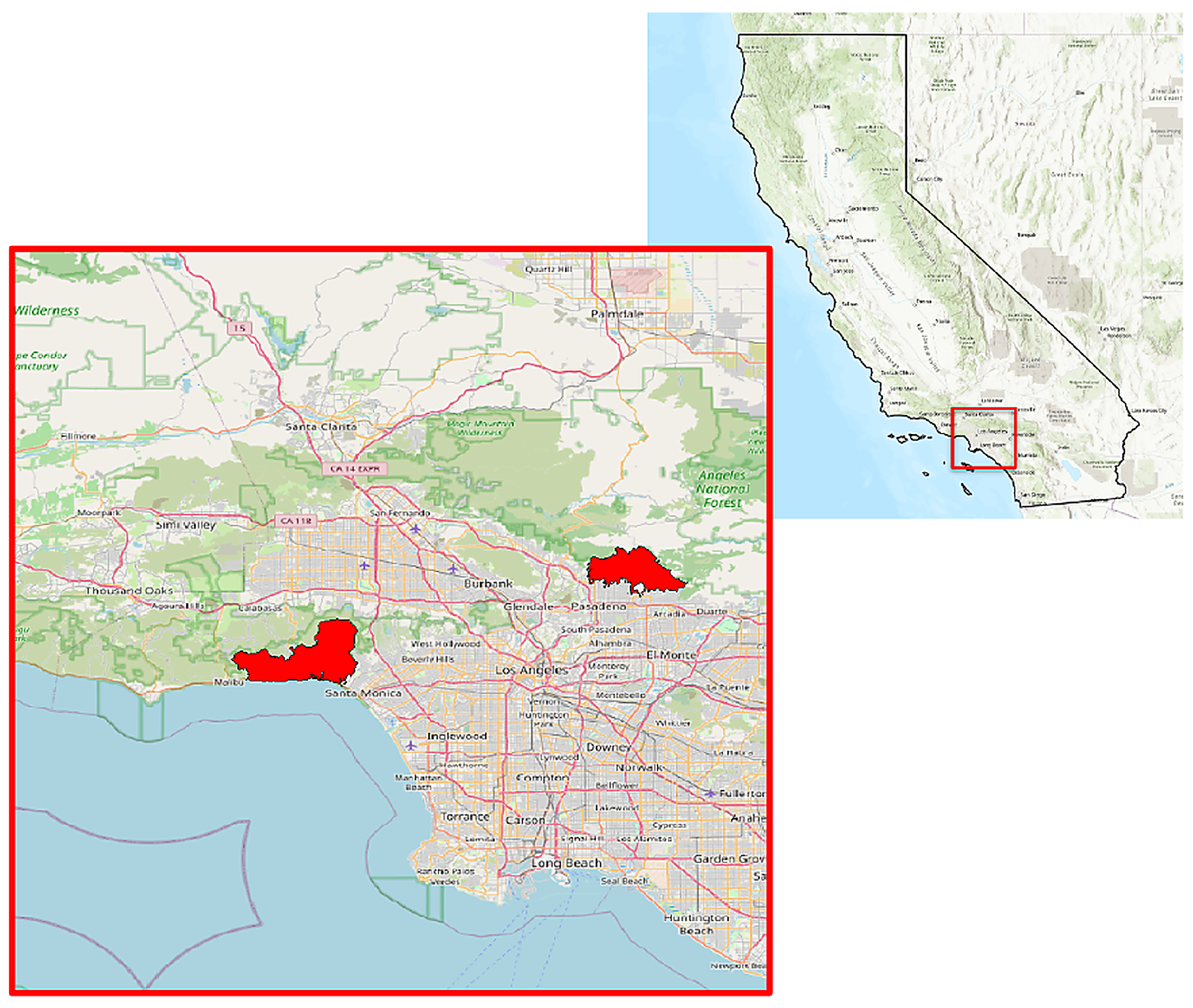
Figure 1.
The 2025 perimeters for Palisades and Eaton fires, within contextual map of California (Source: CALFIRE, OpenStreetMaps).
Figure 1.
The 2025 perimeters for Palisades and Eaton fires, within contextual map of California (Source: CALFIRE, OpenStreetMaps).
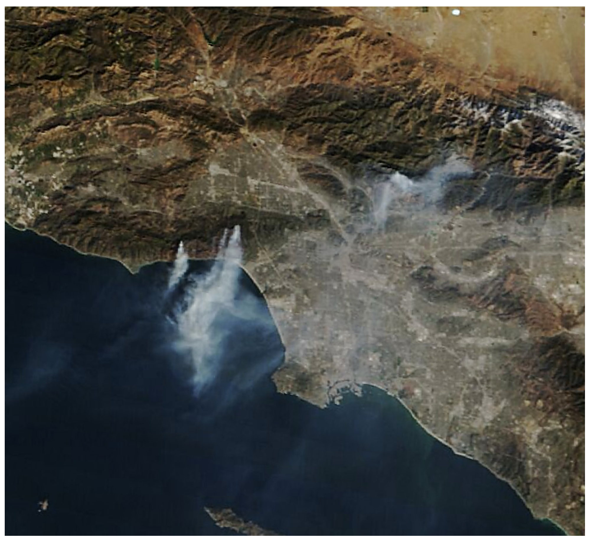
Figure 2.
Satellite image showing the smoke plume directions for the 2025 Palisades and Eaton fires (Source: NASA MODIS, 10 January 2025).
Figure 2.
Satellite image showing the smoke plume directions for the 2025 Palisades and Eaton fires (Source: NASA MODIS, 10 January 2025).
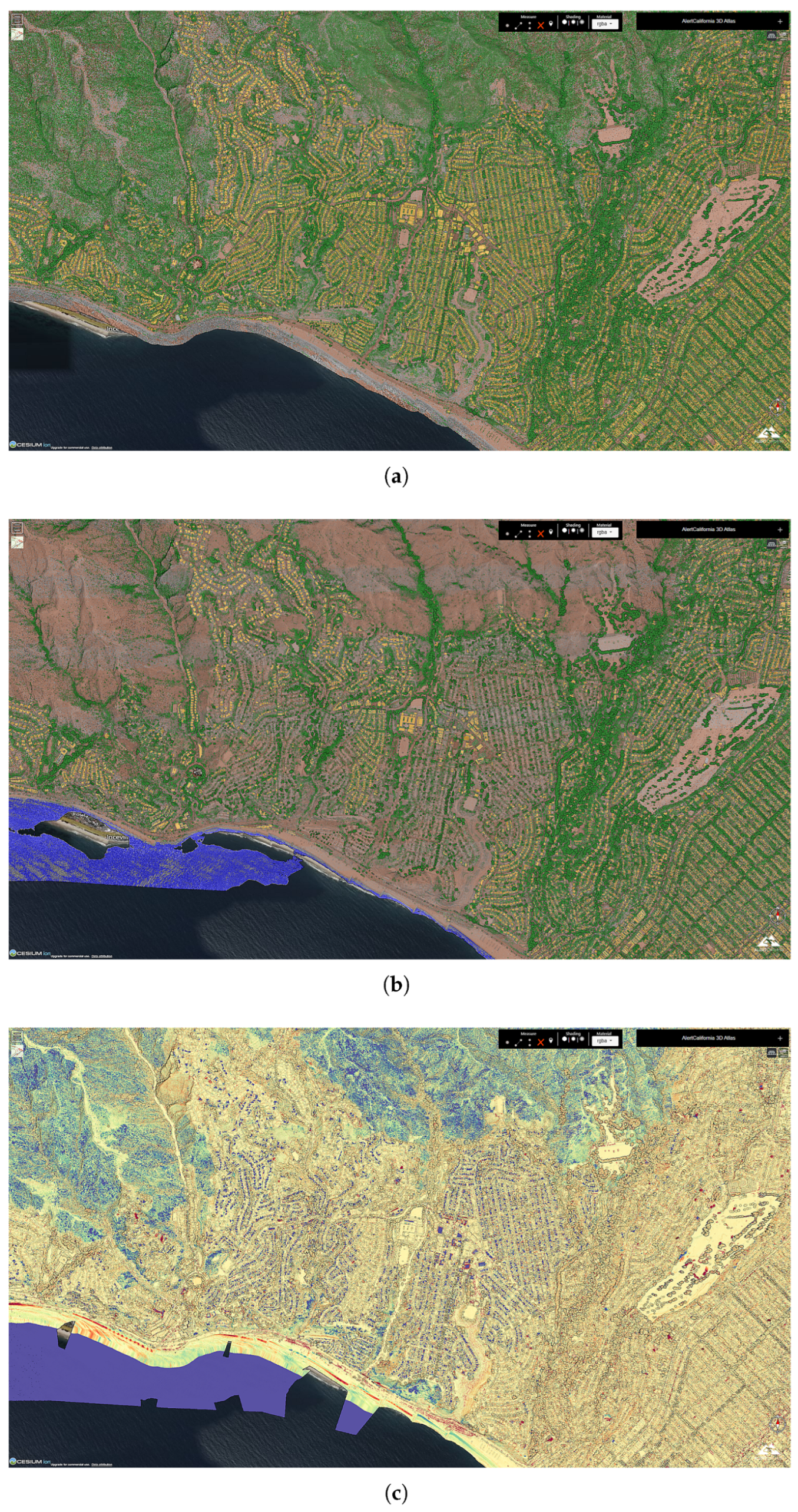
Figure 3.
Showing (a) pre-fire baseline classified LiDAR data from 2023, (b) post-fire classified data from 2025 and (c) a height difference map for 2023–2025, capturing overall change, highlighting areas with vegetation and infrastructure losses. In the classified panels (a,b), vegetation is shown in green, buildings in orange, ground in brown, and unclassified points in grey; in the height difference map (c), a diverging color scale encodes the per-cell change in surface height between the two epochs.
Figure 3.
Showing (a) pre-fire baseline classified LiDAR data from 2023, (b) post-fire classified data from 2025 and (c) a height difference map for 2023–2025, capturing overall change, highlighting areas with vegetation and infrastructure losses. In the classified panels (a,b), vegetation is shown in green, buildings in orange, ground in brown, and unclassified points in grey; in the height difference map (c), a diverging color scale encodes the per-cell change in surface height between the two epochs.
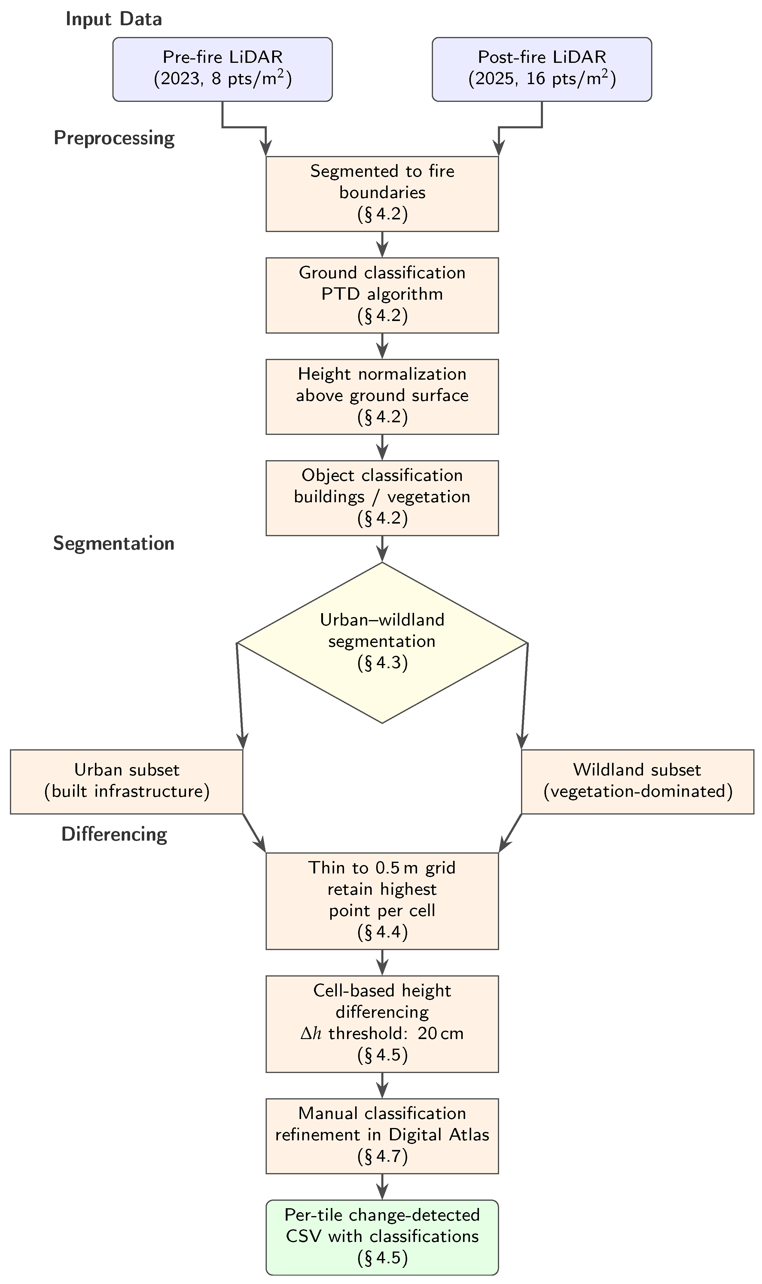
Figure 4.
Data- processing pipeline: from raw multi-temporal LiDAR to change-detected, classified point records. Both pre-fire and post-fire datasets are segmented, classified, and differenced on aligned 0.5 m grids. The output per-tile CSV files serve as input to the summarization and emissions pipeline (
Section 4.5).
Figure 4.
Data- processing pipeline: from raw multi-temporal LiDAR to change-detected, classified point records. Both pre-fire and post-fire datasets are segmented, classified, and differenced on aligned 0.5 m grids. The output per-tile CSV files serve as input to the summarization and emissions pipeline (
Section 4.5).
Figure 5.
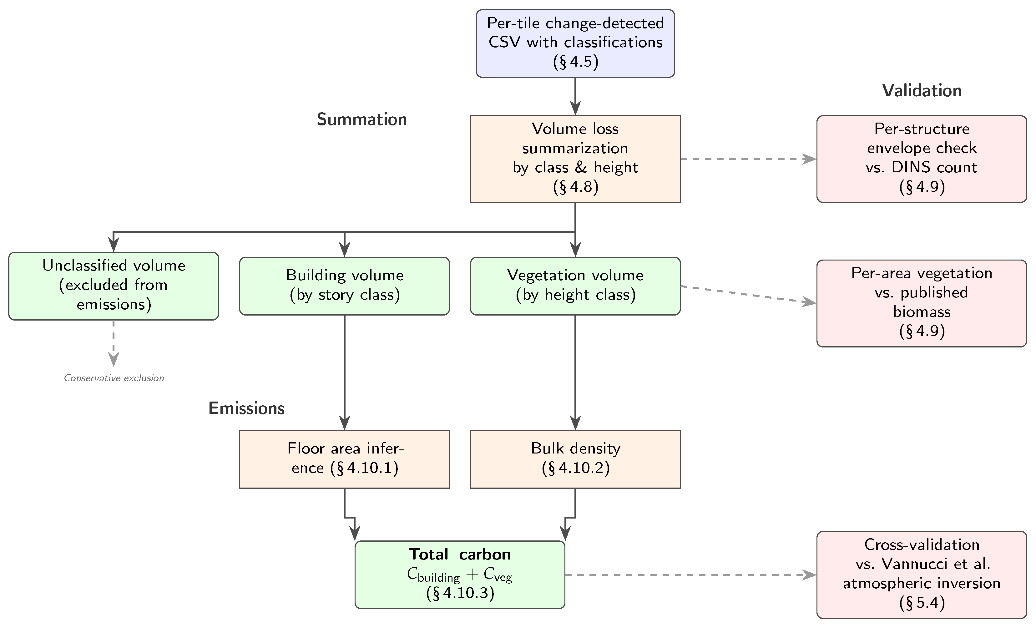
Summarization and carbon emissions pipeline. Change-detected records from the processing pipeline (
Figure 4) are aggregated by classification and height class, then converted to emitted carbon through class-specific pathways. Solid arrows denote the primary data flow through the pipeline, and dashed arrows indicate validation cross-checks against independent estimates. All unclassified categories are excluded from the emissions calculation as a conservative choice (
Section 4.8).
Figure 5.
Summarization and carbon emissions pipeline. Change-detected records from the processing pipeline (
Figure 4) are aggregated by classification and height class, then converted to emitted carbon through class-specific pathways. Solid arrows denote the primary data flow through the pipeline, and dashed arrows indicate validation cross-checks against independent estimates. All unclassified categories are excluded from the emissions calculation as a conservative choice (
Section 4.8).
Figure 6.
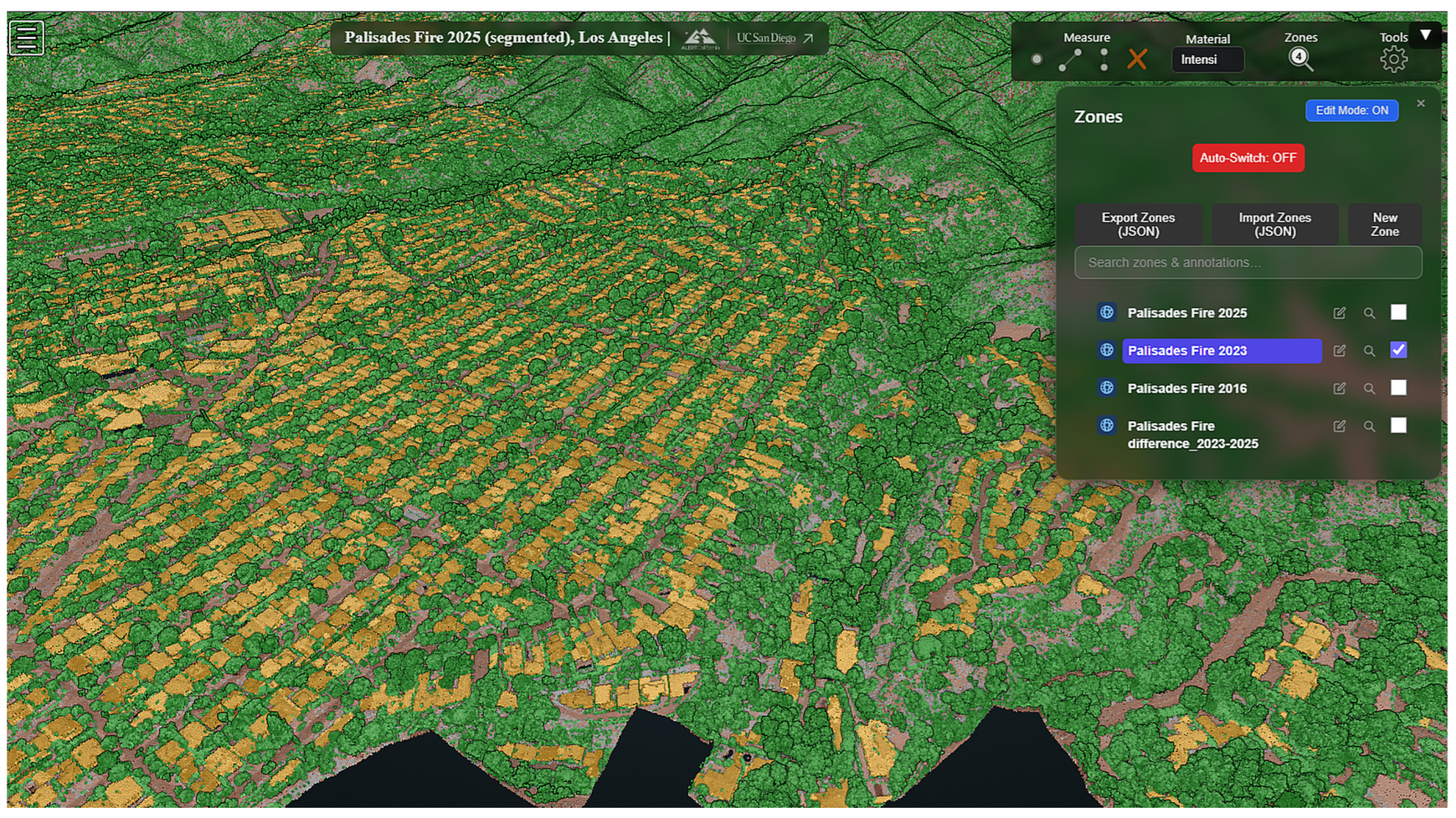
ALERTCalifornia Digital Atlas, based on the Potree WebGL viewer (version 1.8). The full-resolution data is shown in an interactive window, colored by classification and intensity, where vegetation is rendered in green, buildings in orange, ground in brown, and unclassified points in grey. The interface enables switching, reclassification, and segmentation between all data layers in the 4 zones shown in the top-right menu.
Figure 6.
ALERTCalifornia Digital Atlas, based on the Potree WebGL viewer (version 1.8). The full-resolution data is shown in an interactive window, colored by classification and intensity, where vegetation is rendered in green, buildings in orange, ground in brown, and unclassified points in grey. The interface enables switching, reclassification, and segmentation between all data layers in the 4 zones shown in the top-right menu.
Figure 7.
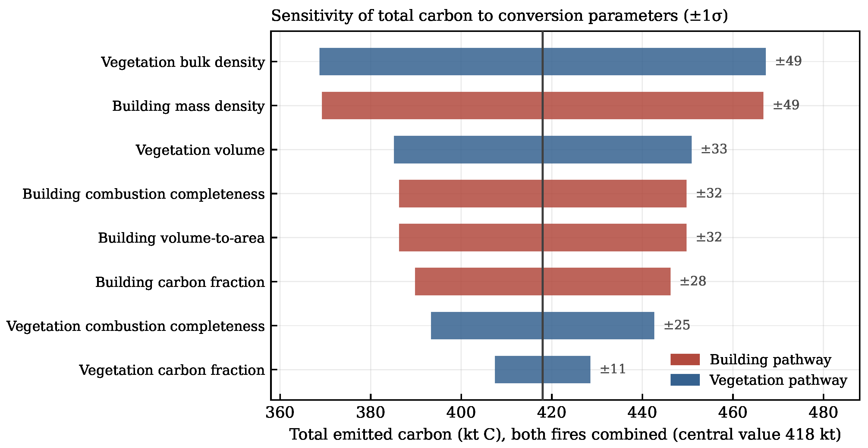
Sensitivity of total emitted carbon (both fires combined; central value 418 kt C) to each conversion parameter, with each varied by about its central value. Vegetation bulk density and building combustible mass density are the dominant contributors.
Figure 7.
Sensitivity of total emitted carbon (both fires combined; central value 418 kt C) to each conversion parameter, with each varied by about its central value. Vegetation bulk density and building combustible mass density are the dominant contributors.
Figure 8.
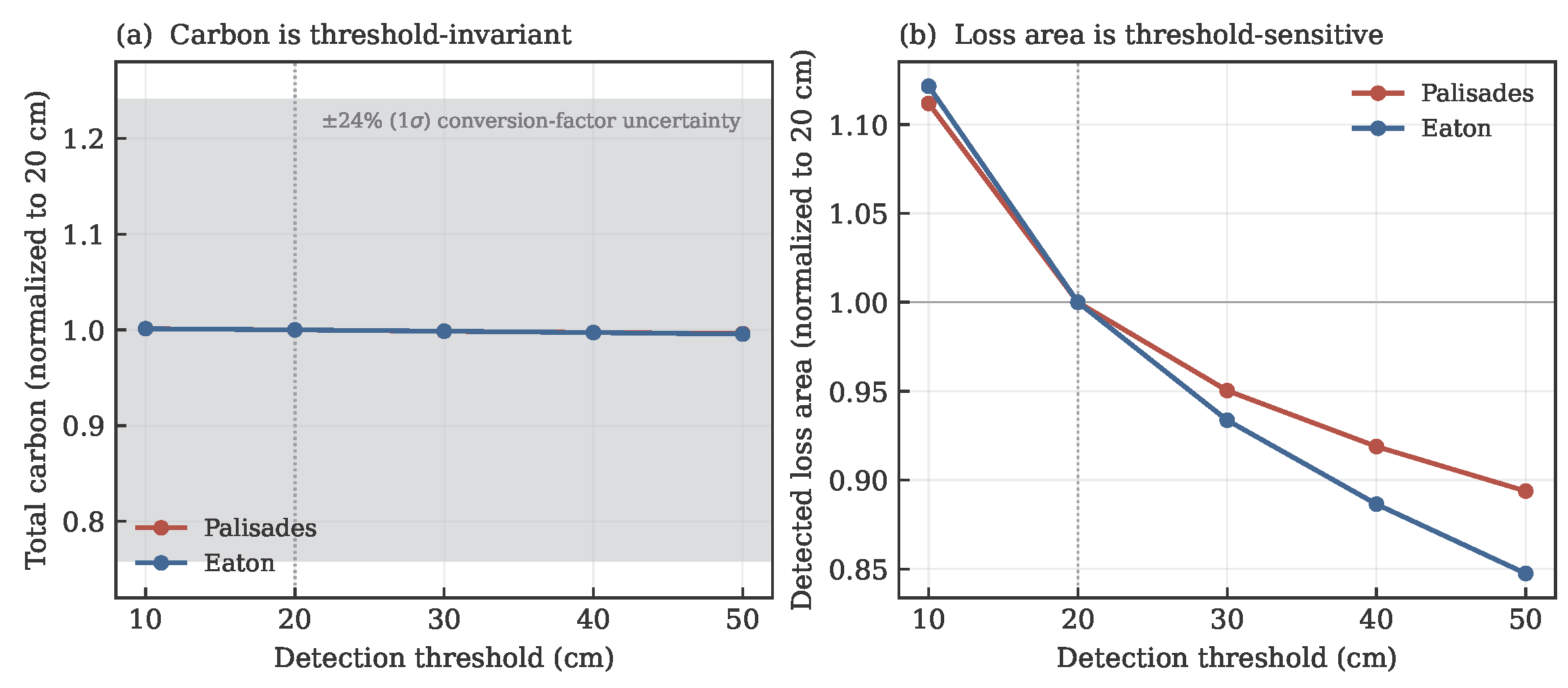
Threshold sensitivity of (a) total emitted carbon and (b) detected loss area, each normalized to the 20 cm baseline. Total carbon varies by less than 1% across the 10–50 cm sweep, well within the ±24% () conversion-factor uncertainty (shaded band), whereas detected loss area is threshold-sensitive. The dashed vertical line marks the 20 cm baseline threshold used throughout the analysis.
Figure 8.
Threshold sensitivity of (a) total emitted carbon and (b) detected loss area, each normalized to the 20 cm baseline. Total carbon varies by less than 1% across the 10–50 cm sweep, well within the ±24% () conversion-factor uncertainty (shaded band), whereas detected loss area is threshold-sensitive. The dashed vertical line marks the 20 cm baseline threshold used throughout the analysis.
Figure 9.
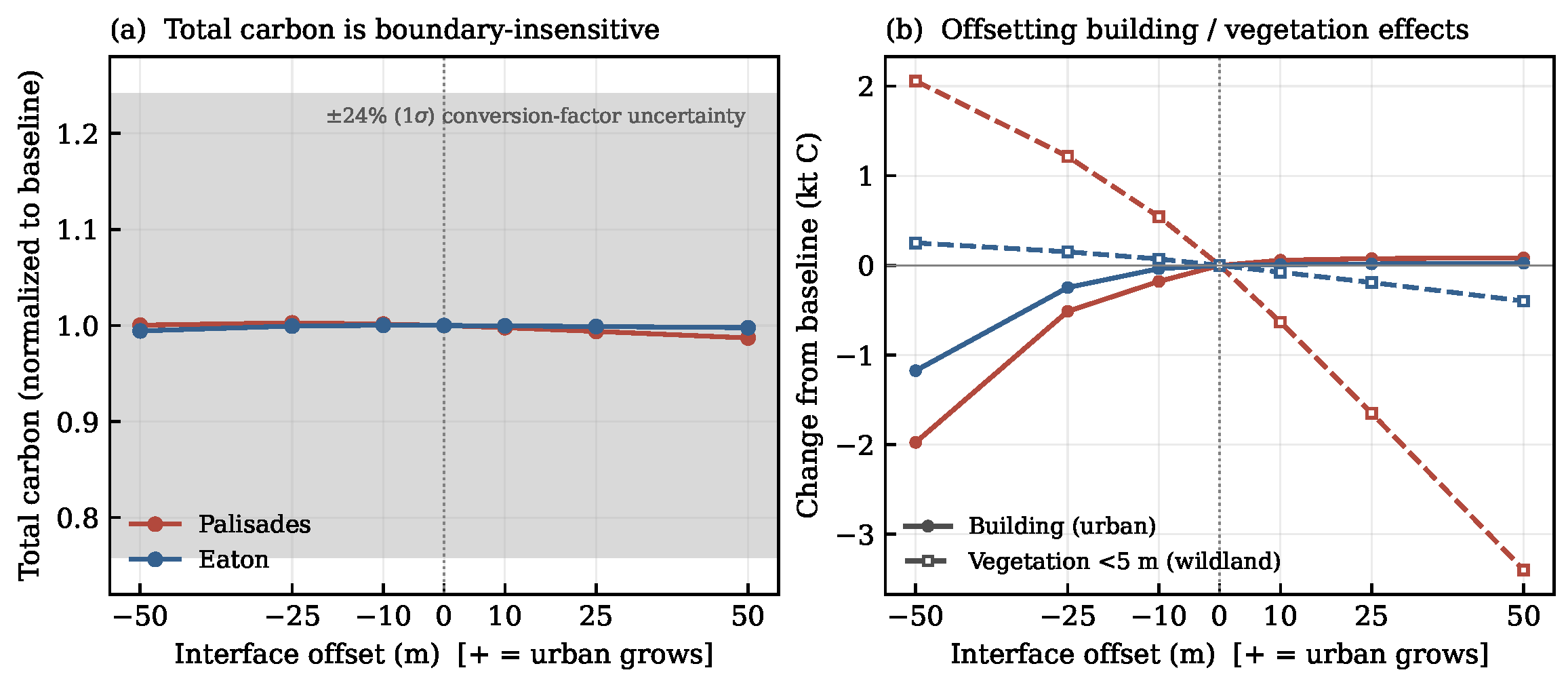
Urban/wildland boundary sensitivity. (a) Total emitted carbon normalized to the baseline boundary versus interface offset (positive = urban zone grows into wildland); variation stays within the ±24% () conversion-factor uncertainty (shaded band). (b) Change from baseline in the building (urban) and sub-5 m vegetation (wildland) carbon pathways, showing the partially offsetting response. In both panels, red denotes the Palisades fire and blue the Eaton fire; in (b), solid lines with filled markers denote the building (urban) pathway and dashed lines with open markers denote the sub-5 m vegetation (wildland) pathway. The vertical dashed line marks the zero-offset baseline boundary.
Figure 9.
Urban/wildland boundary sensitivity. (a) Total emitted carbon normalized to the baseline boundary versus interface offset (positive = urban zone grows into wildland); variation stays within the ±24% () conversion-factor uncertainty (shaded band). (b) Change from baseline in the building (urban) and sub-5 m vegetation (wildland) carbon pathways, showing the partially offsetting response. In both panels, red denotes the Palisades fire and blue the Eaton fire; in (b), solid lines with filled markers denote the building (urban) pathway and dashed lines with open markers denote the sub-5 m vegetation (wildland) pathway. The vertical dashed line marks the zero-offset baseline boundary.
Table 1.
CAL FIRE DINS damage and casualty totals.
Table 1.
CAL FIRE DINS damage and casualty totals.
| Damage Type | Eaton | Palisades |
|---|
| Structures Damaged | 1074 | 973 |
| Structures Destroyed | 9414 | 6837 |
| Confirmed Civilian Fatalities | 18 | 12 |
Table 2.
Source LiDAR datasets.
Table 2.
Source LiDAR datasets.
| USGS Dataset Name | Acquisition Dates | Mean Density |
|---|
| CA_LosAngeles_1_B23 | 8 January 2023–7 January 2024 | 8 pts/m2 |
| CA_LAPostWildfire_Eaton_C25 | 21 January 2025–22 January 2025 | 16 pts/m2 |
| CA_LAPostWildfire_Palisades_C25 | 21 January 2025 | 16 pts/m2 |
Table 3.
Vegetation bulk density assignments.
Table 3.
Vegetation bulk density assignments.
| Height Class | Dominant Community | (kg/m3) |
|---|
| <1 m | Coastal sage scrub/herbaceous | 0.9 |
| 1–5 m | Mixed/chamise chaparral | 2.0 |
| >5 m | Oak woodland/mixed canopy | 3.0 |
Table 4.
Destroyed gross floor area and building carbon emissions. Per-structure mean computed using DINS counts (6837 Palisades, 9414 Eaton). Uncertainty: ().
Table 4.
Destroyed gross floor area and building carbon emissions. Per-structure mean computed using DINS counts (6837 Palisades, 9414 Eaton). Uncertainty: ().
| Fire | 1-Story (m2) | 2-Story (m2) | 3+ (m2) | Total (m2) | Per-Struct. (m2) | C (kt) |
|---|
| Palisades | 484,935 | 1,327,481 | 301,666 | 2,114,082 | 309 | |
| Eaton | 644,982 | 751,200 | 105,336 | 1,501,518 | 160 | |
Table 5.
Vegetation carbon emissions by fire footprint. Under-1 m and 1–5 m classes include wildland-zone volumes only; the over-5 m class includes both wildland and urban zones. Uncertainty: ().
Table 5.
Vegetation carbon emissions by fire footprint. Under-1 m and 1–5 m classes include wildland-zone volumes only; the over-5 m class includes both wildland and urban zones. Uncertainty: ().
| Fire | <1 m (m3) | 1–5 m (m3) | >5 m (m3) | C (kt) | |
|---|
| Palisades | 463 | 91,452,885 | 32,315,777 | 107 | 43 |
| Eaton | 623 | 33,685,476 | 31,319,781 | 57 | 23 |
Table 6.
Per-structure envelope volume validation.
Table 6.
Per-structure envelope volume validation.
| Fire | Building Vol (m3) | DINS Count | Per-Struct. (m3) | In Range? |
|---|
| Palisades | 6,927,736 | 6837 | 1013 | Yes |
| Eaton | 5,184,649 | 9414 | 551 | Yes |
Table 7.
Threshold sensitivity of carbon and detected loss area. Carbon totals vary <1% across the 10–50 cm sweep, far within the ±23–24% () conversion-factor uncertainty; detected loss area is threshold-sensitive.
Table 7.
Threshold sensitivity of carbon and detected loss area. Carbon totals vary <1% across the 10–50 cm sweep, far within the ±23–24% () conversion-factor uncertainty; detected loss area is threshold-sensitive.
| Fire | Thr. (cm) | Building (kt C) | Veg. (kt C) | Total (kt C) | Loss Area (km2) |
|---|
| Palisades | 10 | 148.7 | 107.0 | 255.7 | 66.95 |
| 20 | 148.4 | 107.0 | 255.4 | 60.22 |
| 30 | 148.1 | 106.9 | 255.0 | 57.23 |
| 40 | 148.0 | 106.7 | 254.7 | 55.33 |
| 50 | 147.8 | 106.6 | 254.4 | 53.82 |
| Eaton | 10 | 105.5 | 57.3 | 162.8 | 35.32 |
| 20 | 105.4 | 57.2 | 162.6 | 31.49 |
| 30 | 105.3 | 57.1 | 162.4 | 29.40 |
| 40 | 105.2 | 56.9 | 162.1 | 27.92 |
| 50 | 105.2 | 56.7 | 161.9 | 26.69 |
Table 8.
Urban/wildland boundary-placement sensitivity. The interface is offset in/out by up to ±50 m (positive = urban grows into wildland; coastline and fire-perimeter edges held fixed). Total carbon varies by less than 1.4% for either fire, within the ±23–24% () conversion-factor uncertainty.
Table 8.
Urban/wildland boundary-placement sensitivity. The interface is offset in/out by up to ±50 m (positive = urban grows into wildland; coastline and fire-perimeter edges held fixed). Total carbon varies by less than 1.4% for either fire, within the ±23–24% () conversion-factor uncertainty.
| Fire | Offset (m) | Building (kt C) | Veg. (kt C) | Total (kt C) |
|---|
| Palisades | | 146.4 | 109.0 | 255.5 |
| 147.9 | 108.2 | 256.1 |
| 148.2 | 107.5 | 255.8 |
| 0 | 148.4 | 107.0 | 255.4 |
| 148.5 | 106.4 | 254.8 |
| 148.5 | 105.3 | 253.8 |
| 148.5 | 103.6 | 252.1 |
| Eaton | | 104.2 | 57.5 | 161.7 |
| 105.2 | 57.4 | 162.5 |
| 105.4 | 57.3 | 162.6 |
| 0 | 105.4 | 57.2 | 162.6 |
| 105.4 | 57.1 | 162.5 |
| 105.4 | 57.0 | 162.4 |
| 105.4 | 56.8 | 162.2 |
Table 9.
Accuracy-assessment sampling design: per-stratum population, area weight, and sample size (pooled across both fires).
Table 9.
Accuracy-assessment sampling design: per-stratum population, area weight, and sample size (pooled across both fires).
| Class | Zone | Population (Cells) | Weight | Sample n |
|---|
| Building | Urban | 12,497,621 | 0.034 | 100 |
| Building | Wildland | 62,736 | 0.0002 | 50 |
| Vegetation | Urban | 40,825,297 | 0.111 | 100 |
| Vegetation | Wildland | 254,478,813 | 0.694 | 175 |
| Unclassified | Urban | 6,943,051 | 0.019 | 100 |
| Unclassified | Wildland | 52,023,661 | 0.142 | 125 |
| Total | | 366,831,179 | 1.000 | 650 |
Table 10.
Classification confusion matrix for the retained loss cells (2023 class assignment; ). Rows are the mapped class; columns are the reference (true) class. Raw overall accuracy 99.2%; area-weighted overall accuracy 99.9% (±0.2); . UA: user’s accuracy; PA: producer’s accuracy (raw sample counts).
Table 10.
Classification confusion matrix for the retained loss cells (2023 class assignment; ). Rows are the mapped class; columns are the reference (true) class. Raw overall accuracy 99.2%; area-weighted overall accuracy 99.9% (±0.2); . UA: user’s accuracy; PA: producer’s accuracy (raw sample counts).
| Mapped | Reference | Total | UA |
|---|
| Building | Vegetation | Unclassified |
|---|
| Building | 146 | 2 | 2 | 150 | 97.3% |
| Vegetation | 0 | 274 | 1 | 275 | 99.6% |
| Unclassified | 0 | 0 | 225 | 225 | 100.0% |
| Total | 146 | 276 | 228 | 650 | |
| PA | 100.0% | 99.3% | 98.7% | | |
Table 11.
Error-adjusted loss areas for the retained inventory, following Olofsson et al. [
48]. Adjusted areas differ from the mapped areas by less than 0.15 km
2.
Table 11.
Error-adjusted loss areas for the retained inventory, following Olofsson et al. [
48]. Adjusted areas differ from the mapped areas by less than 0.15 km
2.
| Class | Mapped (km2) | Adjusted (km2) | 95% CI (km2) |
|---|
| Building | 3.14 | 3.14 | <0.01 |
| Vegetation | 73.83 | 73.72 | ±0.20 |
| Unclassified | 14.74 | 14.84 | ±0.20 |
Table 12.
Inter-epoch vertical co-registration on stable hard-surface control points. Bias is the mean (2025 minus 2023) elevation difference; RMSE is the root-mean-square difference; n is the number of the 40 sampled control points per fire that matched a cloud point within 1 m in both epochs.
Table 12.
Inter-epoch vertical co-registration on stable hard-surface control points. Bias is the mean (2025 minus 2023) elevation difference; RMSE is the root-mean-square difference; n is the number of the 40 sampled control points per fire that matched a cloud point within 1 m in both epochs.
| Fire | n | Bias (cm) | 95% CI (cm) | RMSE (cm) |
|---|
| Palisades | 37 | | to | 6.55 |
| Eaton | 27 | | to | 6.89 |
| Pooled | 64 | −5.84 | −6.67 to −5.02 | 6.70 |