


Highlights
What are the main findings?
- A conditional generative adversarial network generated continuous 10 m day–night land surface temperature across four peri-urban areas. Centered RMSE against same-date Landsat was 1.03–2.38 °C at 30 m, against 3.18–3.36 °C for interpolation of the 1 km input, and the nighttime field was validated independently against ECOSTRESS at 70 m.
- Against a 25-year land-cover-stratified climatology, the Relative Diurnal Thermal Index reveals built-up surfaces retaining heat more strongly than cropland in all four cities (Cohen’s d 0.54–1.67) and separates the two significantly.
What are the implications of the main findings?
- Land-cover-stratified climatological normalization resolves an otherwise inconsistent diurnal signal into a consistent urban heat-retention signature, providing a field-scale, diurnal complement to coarse-resolution or daytime-only UHI indicators.
- RDTI correlates at −0.29 to −0.80 with a rate-matched SUHII proxy while remaining distinct, by design, from absolute-temperature hot-spot methods, indicating potential for peri-urban climate-adaptation planning.
Abstract
Existing urban heat island (UHI) indicators are typically coarse in resolution, limited to daytime acquisitions, or computed without reference to land cover, and cannot resolve field-scale diurnal behavior. This study introduces the Relative Diurnal Thermal Index (RDTI), a dimensionless, land-cover-stratified anomaly computed from daily 10 m day–night land surface temperature (LST) pairs. A conditional generative adversarial network fused daily 1 km MODIS day/night LST with Landsat-8/9 and Sentinel-2 imagery to generate continuous 10 m LST across four temperate French metropolitan peripheries (Paris, Lille, Nantes, and Bordeaux). RDTI expresses the observed diurnal temperature range as a standardized anomaly against a 25-year (2000–2025) MODIS climatology stratified by land-cover class, so each pixel is referenced to the historical behavior of its own surface type. The generated LST was validated against same-date Landsat with centered RMSE of 1.03–2.38 °C, against 3.18–3.36 °C for interpolation of the coarse input, and outperformed TsHARP and random-forest downscaling in three of four cities; the nighttime field was validated independently against ECOSTRESS at 70 m, reproducing the built–cropland thermal contrast to within 0.052 °C. Once normalized against class-specific climatology, built-up surfaces showed suppressed nocturnal cooling relative to cropland in all four cities (Cohen’s d 0.54–1.67). RDTI correlates at −0.29 to −0.80 with relative-warmth SUHII surfaces while remaining distinct, by design, from absolute-temperature hot-spot methods, providing a field-scale, climatologically grounded diurnal complement to existing UHI indicators.
1. Introduction
Urban heat islands (UHIs) describe the systematic elevation of temperature in built-up areas relative to their surroundings [1], driven by impervious surfaces, reduced albedo, and the high heat capacity of construction materials [2]. These materials absorb heat during the day and release it slowly after sunset [3]. The thermal contrast between cities and their surroundings is typically strongest at night [4]. As urban areas expand globally, UHI intensity tends to scale with city size and density [5], making it an increasingly widespread feature of the urban climate.
In peri-urban zones, this thermal contrast extends into the surrounding landscape [6]. As cities expand into adjacent open land, those areas are increasingly exposed to higher nighttime temperatures from neighboring built-up surfaces [6,7]. At the same time, vegetated land is not passive: through evapotranspiration, vegetated surfaces actively influence the local thermal environment [6]. The urban/rural boundary therefore functions as a zone of mutual thermal influence, where the direction and strength of heat exchange depend on land cover and time of day [6].
In temperate regions, this interaction is intensified by climate change [8]. Heatwaves are becoming more frequent and intense [9]. Their effects are compounded where built-up surfaces retain heat overnight and suppress the nocturnal temperature decline that characterizes the undisturbed landscape. Temperate landscapes are characterized by a dense, fragmented mosaic of urban and open land uses, often with short distances between built-up cores and surrounding land [6], a configuration where even moderate UHI effects can propagate efficiently outward, while the local thermal response remains highly localized [6].
A range of remote sensing approaches has been developed to characterize UHIs [4]. These include statistical thresholding of land surface temperature (LST) to delineate anomalously warm pixels [10]; zone-based methods computing the contrast between predefined urban and rural areas [5]; and approaches relating LST to spectral indices through correlation or regression [11]. Complementary indicators have also been proposed, including UHI Intensity based on air temperature contrasts [12], the Urban Thermal Field Variance Index based on normalized LST anomalies [13], Surface UHI Intensity based on urban–rural LST differences [5], and the raw Diurnal Temperature Range derived from day/night LST pairs [14].
However, these approaches share recurring limitations for field-scale assessment [4]. Many operate at coarse resolution insufficient to resolve individual parcels or sharp gradients across land-cover boundaries [12]. Several rely on single daytime acquisitions, missing the nocturnal dynamics in which the urban thermal signature is strongest [14]. Others depend on fixed urban/rural zones or climatological averages computed without reference to land cover, masking the heterogeneity of peri-urban landscapes [5,6]. To the authors’ knowledge, no existing LST-based indicator expresses a land-cover-stratified pixel-level temporal anomaly at sub-field resolution on day/night LST pairs.
To address these limitations, this study proposes the Relative Diurnal Thermal Index (RDTI), a dimensionless, land-cover-stratified index computed from daily 10 m day/night LST pairs. RDTI expresses the observed diurnal temperature range as a pixel-level anomaly relative to a land-cover-stratified climatological baseline, so that each pixel is evaluated against the historical norm of its own surface type [6]. Negative values indicate sustained heat retention, and positive values indicate thermal relief [14]. By operating continuously at 10 m without fixed zones, single-scene snapshots, or land-cover-blind averages, RDTI aims to provide a field-scale description of diurnal thermal behavior applicable to urban thermal management and to the surrounding peri-urban landscape.
Two hypotheses guide this study:
- A generative adversarial network (GAN)-based fusion of daily 1 km MODIS day/night LST with Landsat and Sentinel-2 imagery may generate continuous 10 m LST time series capable of resolving field-scale diurnal dynamics in heterogeneous peri-urban landscapes.
- The resulting RDTI may offer advantages over existing UHI indicators by capturing nocturnal dynamics and revealing field-scale heterogeneity that coarse-resolution or daytime-only metrics cannot.
These hypotheses drive the development of a high-resolution diurnal UHI assessment framework with potential applications to peri-urban climate-adaptation planning.
2. Materials and Methods
2.1. Study Area
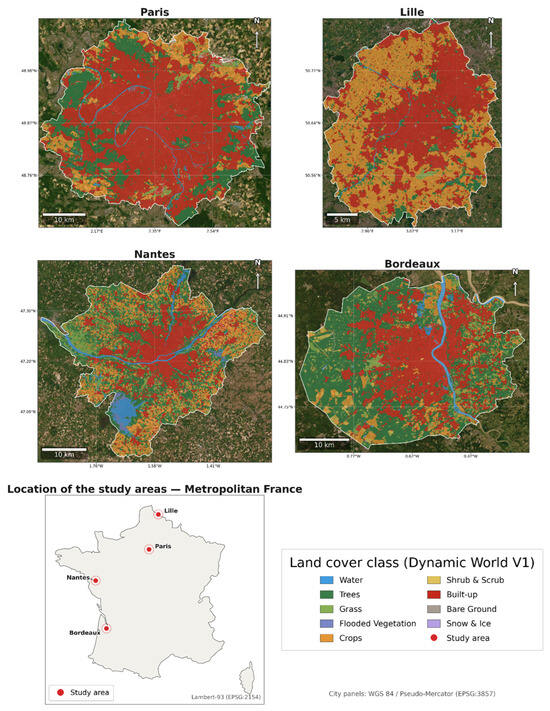
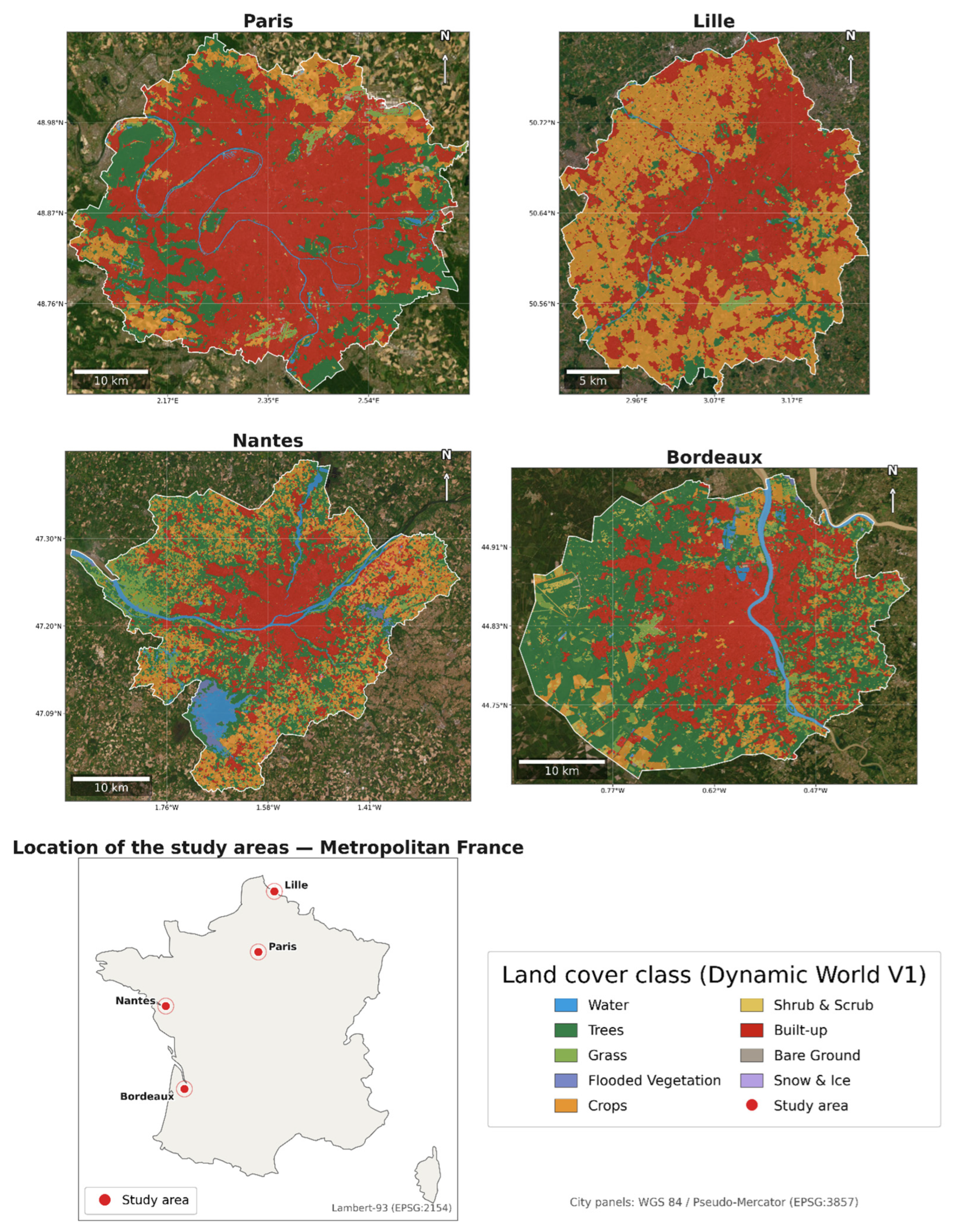
This study examines peri-urban agricultural landscapes across temperate France, defined here as the northern and western regions under an oceanic to semi-continental climate [15]. This zone (Figure 1) encompasses the major metropolitan peripheries of Paris, Lille, Nantes, Bordeaux, and associated urban agglomerations, where ongoing urban expansion interacts directly with intensive farmland systems [16]. Together, the four metropolitan peripheries cover a combined study extent of approximately 4500 km2.
Figure 1.
Study area covering four metropolitan peripheries of temperate France: Paris, Lille, Nantes and Bordeaux. Paris ≈ 1560 km2, Lille ≈ 680 km2, Nantes ≈ 1080 km2, Bordeaux ≈ 1100 km2.
Climatically, this area is characterized by mild winters, moderate annual precipitation, and a documented rise in the frequency and intensity of summer heatwaves linked to accelerating climate change [8]. These conditions amplify UHI effects, particularly at night, in the transition zones between built-up areas and surrounding croplands [17].
Agriculturally, the peri-urban belts of temperate France support a heterogeneous mosaic of high-value production systems, including dominant wheat rotations on arable land and vineyards [18]. These landscapes contribute to local thermal regulation through elevated evapotranspiration, yet they face systematic pressure from urban sprawl: France artificializes approximately 50,000–55,000 ha of agricultural land annually, with the majority occurring in peri-urban fringes around temperate metropolitan regions [16].
This scope reflects the broader temperate dynamics described in the introduction, with sufficient diversity in crop types and urban/rural configurations to support a robust field-scale assessment. The diversity of crop types and urban/rural configurations across these regions enables a robust assessment of UHI/agriculture interactions under real-world heterogeneous conditions.
2.2. Datasets
The analysis relied on a multi-sensor satellite data stream that combines high temporal resolution thermal data with high spatial resolution optical imagery for cGAN training and downscaling, complemented by in situ meteorological records (Table 1).
Table 1.
Datasets used in this study.
Daily 1 km MODIS day and night LST products provided the temporal backbone: MODIS/Terra daytime LST (MOD11A1) and MODIS/Aqua nighttime LST (MYD11A1), chosen so that each acquisition captures the near-peak daytime heating (Terra, ~10:30 local overpass) and the pre-dawn radiative-cooling minimum (Aqua, ~01:30 local overpass). Sentinel-2 Level-2A scenes served as the primary high-resolution (10 m) reference for GAN-based spatial downscaling, while Landsat-8/9 Collection 2 data were used as the midpoint in the downscaling chain and as the primary validation LST product.
2.3. Methodology
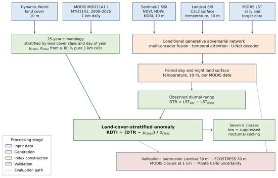
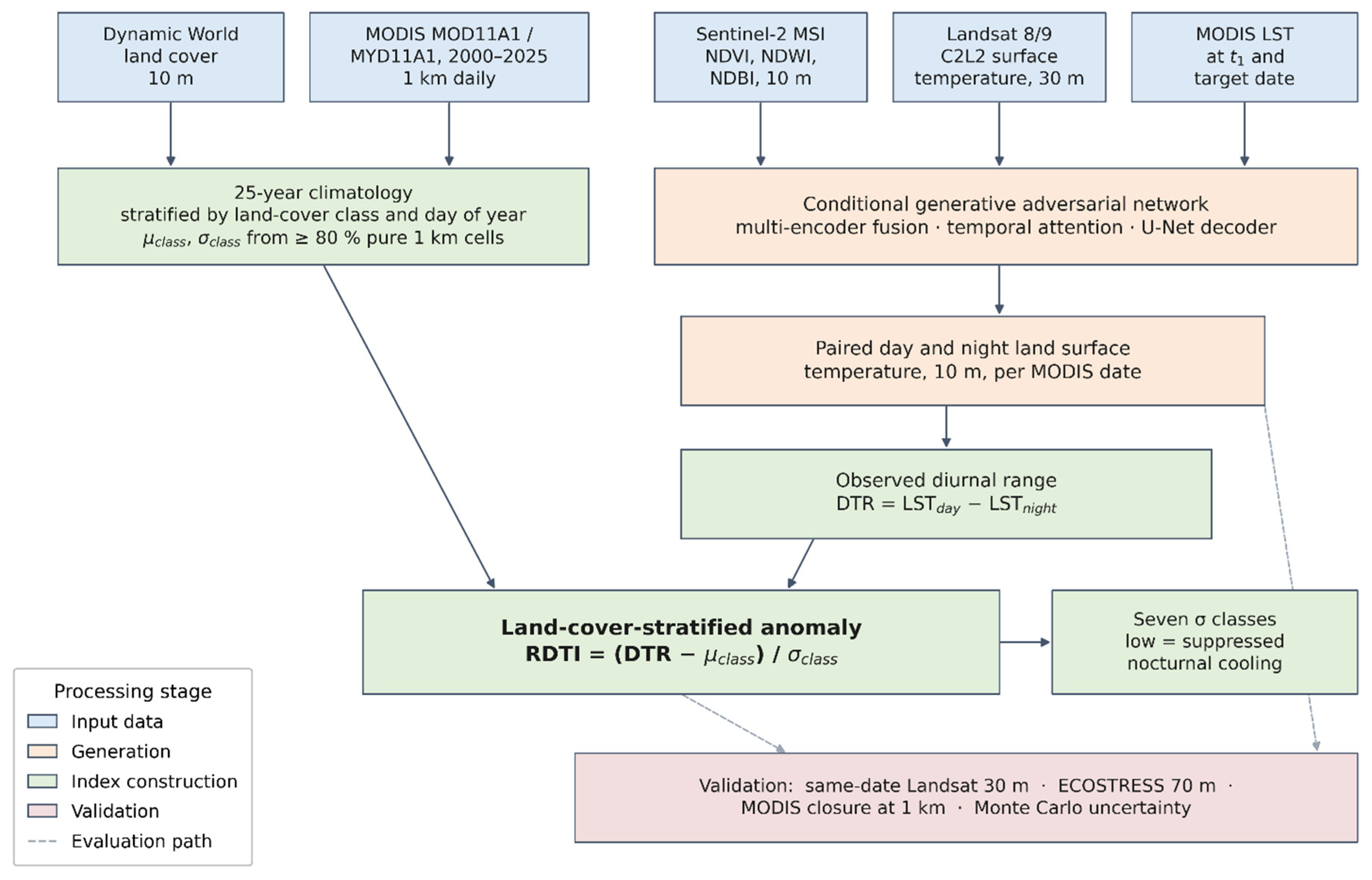
To provide a rigorous benchmark for the proposed approach, the three principal methods currently dominating the UHI literature were first implemented exactly as described in the referenced studies and on the data that the RDTI was implemented on as shown in Figure 2. These methods were then compared against the new RDTI.
Figure 2.
Workflow. Sentinel-2, Landsat and MODIS observations are fused by the generative network to produce paired day and night land surface temperature at 10 m; the diurnal range is then normalized against a land-cover-stratified 25-year MODIS climatology to give the index. Dynamic World land cover enters at the stratification step, not at generation. Dashed lines indicate evaluation paths.
2.3.1. GAN-Based Daily 10 m LST Generation
To overcome the temporal gap inherent in Landsat data while preserving the 10 m spatial detail from Sentinel required for field-scale analysis, a conditional GAN framework was implemented to fuse daily 1 km MODIS day and night LST with Sentinel-2 reference scenes and Landsat-8/9 as a midpoint in the spatial downscaling chain. The approach is adapted from the FuseTen/Weakly-Supervised Generative Network framework [20], which to the best of the authors’ knowledge represents the first non-linear generative method designed specifically for spatio-temporal fusion of LST at 10 m resolution.
LST was first corrected in GEE to ensure accurate representation of surface thermal conditions. LST correction is based on methodology outlined in [21], applying specific corrections to the Landsat-8 thermal band (Band 10) before implementing the GAN approach:
- Cloud Masking: Clouds were masked using ee.Algorithms.Landsat.simpleCloudScore with a 10% threshold, excluding contaminated pixels via ee.Image.updateMask (cloudy pixels and cloud shadow).
- Emissivity Correction: Surface emissivity was estimated from 10 m NDVI-derived fractional vegetation cover (Fv).
- Local Time Difference Correction: Solar declination angle (δ) was adjusted for local time based on longitude and acquisition timestamp.
- Cosine of Zenith Angle: Solar zenith angle cosine (cos(θz)) was calculated to account for illumination effects.
- Zenith Angle Correction for Flat Surfaces: Applied uniformly using solar zenith angle.
- Solar Zenith Angle: Integrated into the radiative transfer model to adjust solar radiation.
2.3.2. GAN Architecture
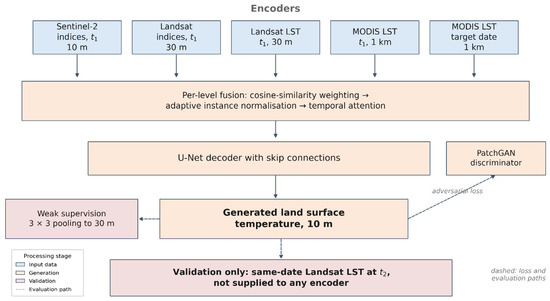
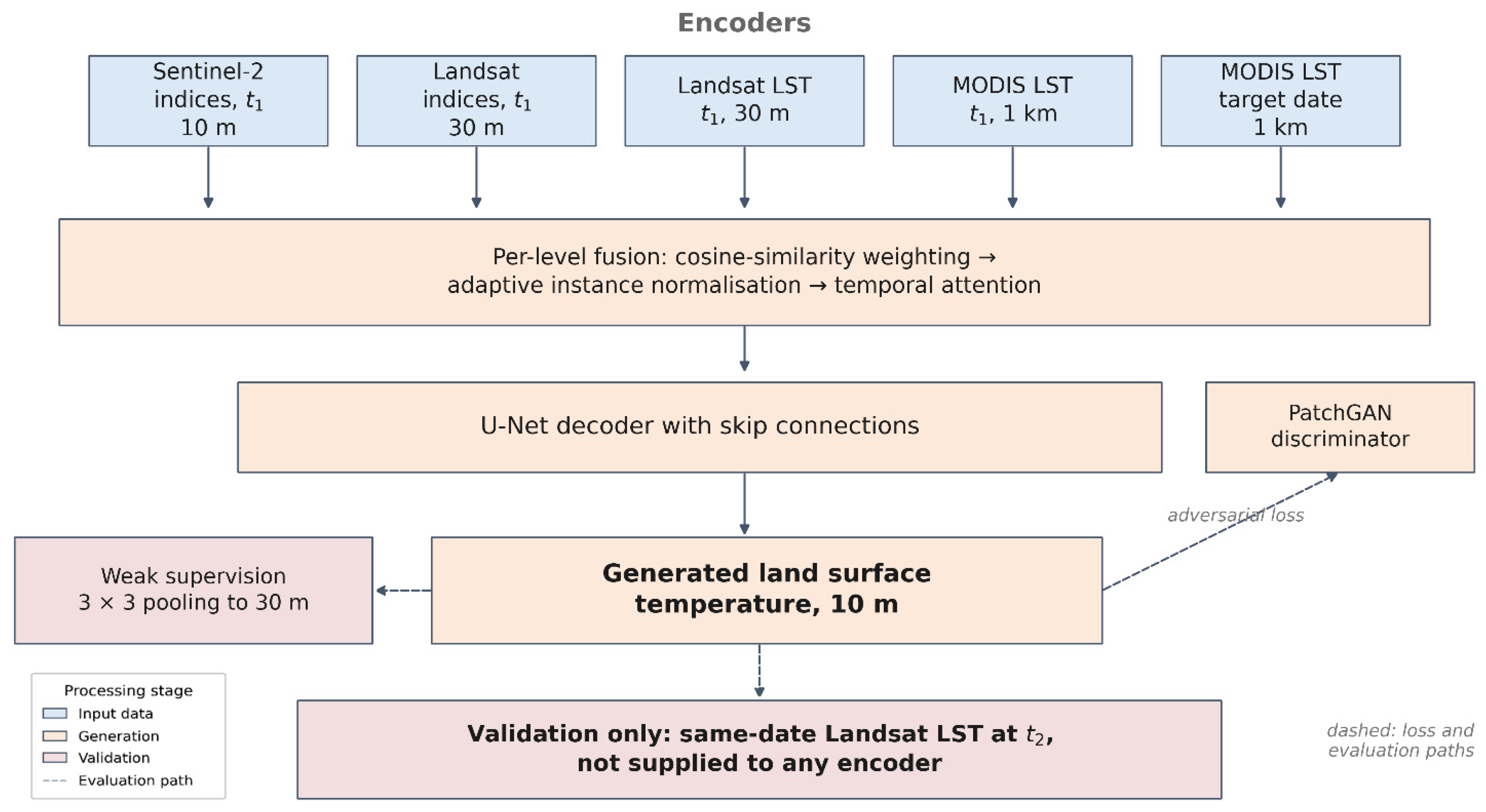
The generator (Figure 3) is structured around five parallel convolutional encoders that independently process:
Figure 3.
Network architecture. Five encoders receive Sentinel-2 indices, Landsat indices and Landsat land surface temperature at t1, and MODIS land surface temperature at t1 and at the target date. Features are fused per level by cosine-similarity weighting, adaptive instance normalization and temporal attention, then decoded through a U-Net with skip connections. The same-date Landsat observation at t2 is used for validation only and is not supplied to any encoder. Dashed lines indicate loss and evaluation paths.
- Sentinel-2 spectral indices: Normalized Difference Vegetation Index (NDVI), Normalized Difference Water Index (NDWI), and Normalized Difference Built-up Index (NDBI) at 10 m at the reference date t1.
- Landsat-8 spectral indices: NDVI, NDWI, NDBI at 30 m at t1.
- Landsat-8 LST at 30 m at t1. The same-date Landsat observation at the target date t2 is used for validation only and is not supplied to any encoder.
- MODIS LST at 1 km at t1.
- MODIS LST at 1 km at the target date t2, which acts as the temporal conditioning signal.
Each encoder applies five levels of progressive downsampling through strided convolutions and residual blocks, producing multi-scale feature maps.
At each encoder level, three fusion operations are applied sequentially:
- A cosine similarity weighting between the Sentinel-2 and Landsat-8 index feature maps spatially refines the Landsat LST features, exploiting the higher spatial resolution of the optical data to guide the thermal representation.
- Adaptive instance normalization [22] aligns the statistical distribution of the MODIS t2 features to those of the refined Landsat LST features, harmonizing the spatial characteristics from Sentinel-2 and Landsat-8 with the temporal signal carried by MODIS.
- A temporal attention mechanism learns a per-pixel weighting between the t1 and t2 feature maps, allowing the model to prioritize the most informative temporal source at each location.
The fused multi-scale features are decoded through a U-Net architecture combining transposed convolutions and residual skip connections, reconstructing the full 10 m LST map at the target date. A Gaussian smoothing filter (σ = 1) is applied as a final post-processing step to suppress high-frequency artefacts introduced by the convolutional layers.
The discriminator follows a PatchGAN design [23], conditioned on the MODIS LST at t2 as thermal context, and outputs a per-patch realness probability. During training, the discriminator receives either the observed Landsat-8 LST (real) or the spatially averaged model output (fake), both concatenated with the MODIS conditioning image. Since no ground truth at 10 m resolution exists, supervision is achieved through an averaging-based strategy: the generated 10 m LST is downsampled to 30 m by a 3 × 3 average pooling operation and compared directly against the Landsat-8 LST at t2 [20]. The total generator loss combines an adversarial term and a pixel-wise L1 term weighted by λ = 100.
Importantly, two independent models were trained: one conditioned on MODIS daytime LST (MOD11A1) and one on MODIS nighttime LST (MYD11A1), reflecting the fundamentally distinct spatial patterns and thermal drivers of daytime and nighttime surface temperatures. Mixing both acquisition times within a single model would combine solar-driven heating dynamics with nocturnal radiative cooling processes, degrading prediction accuracy for both.
Training data were extracted from each city by pairing a cloud-minimized reference date (t1, coinciding with a Landsat-8 acquisition) with a target date (t2, the latest available cloud-minimized Landsat-8 scene), yielding approximately 123,000 training patches across all four cities. Each image was tiled into overlapping 96 × 96 pixel patches (stride = 24 pixels) with random horizontal and vertical flips and 90° rotations applied for augmentation. To avoid memory overflow under Colab’s RAM constraints, the dataset was implemented in a lazy loading scheme that stores full normalized image arrays and extracts patches on-the-fly during training, as opposed to pre-materializing all patches simultaneously. Both the day and night models were trained for 100 epochs using the Adam optimizer (learning rate = 2 × 10⁻⁴, β1 = 0.5, β2 = 0.999) with cosine annealing, a batch size of 16, and model checkpoints saved to Google Drive every 10 epochs. Inference was performed using a sliding window with stride = 48 pixels, with overlapping regions averaged and Gaussian-smoothed (σ = 1) to produce seamless full-scene 10 m LST GeoTIFFs for every available MODIS acquisition date between t1 and t2, saved in the original geographic projection for downstream analysis.
The generated 10 m LST at the target date t2 was validated by resampling it to 30 m (3×3 mean pooling) and comparing it, within the study polygon, against the same-date Landsat LST acquisition. For each city, root mean square error (RMSE), mean absolute error (MAE), bias, Pearson correlation (r), coefficient of determination (R2), structural similarity (SSIM), peak signal-to-noise ratio (PSNR), and ERGAS were computed. As an additional test of whether the generated field contributes genuine fine-scale information rather than reproducing the coarse input, the GAN RMSE was compared against bicubic and bilinear upsampling of the 1 km MODIS conditioning layer to the same 30 m grid. Because no coincident high-resolution nighttime thermal reference exists over the study areas, this same-date Landsat comparison could be performed only for the daytime model as no LST from Landsat is available at night.
2.3.3. Literature Benchmark Methods
To provide a rigorous benchmark for the RDTI, three methods currently dominating the UHI literature were implemented as described in the original referenced studies and applied to the same 10 m LST stack produced by the cGAN, ensuring spatial comparability across all approaches.
- Method 1—LST-based spatial pattern analysis and statistical thresholding [10]
For each daily scene in the GAN-derived 10 m LST stack, the scene-wide mean (μ) and standard deviation (σ) were computed across all valid pixels. Pixels exceeding μ + 1.5σ were flagged as moderate UHI cores; those exceeding μ + 2σ as strong or extreme UHI cores, producing statistically defined thermal “island” polygons for each date. Hot-spot significance was assessed using the Getis–Ord G* spatial statistic: pixels with a local z-score > +1.96 (p < 0.05) surrounded by similarly elevated values were classified as significant UHI clusters, while z < −1.96 identified statistically significant freshness islands. UHI boundaries were delineated objectively along radial transects from each urban center by locating zero-crossings of the second derivative of LST, with boundaries drawn at inflection points ± 2–3 °C. Finally, a temporal persistence index was computed for each pixel as the proportion of study-period dates on which nighttime LST exceeded μ + 1.5σ; pixels with persistence above 70% were classified as persistent UHI cores. This method characterizes UHI as a spatially defined, statistically consistent feature but treats it as temporally static, with no mechanism for isolating events of sustained thermal stress.
- Method 2—Surface Urban Heat Island Intensity (SUHII) quantification [24]
Urban zones were delineated using a combination of land-cover classification derived from cloud-free Sentinel-2 scenes (NDBI > 0.2 and NDVI < 0.2 indicating built-up surface dominance) and administrative boundary cross-referencing. Rural reference zones were defined as agricultural parcels or dense vegetation patches located more than 10–15 km from the urban edge, selected to minimize contamination from urban thermal plumes. SUHII was then computed for each acquisition date as:
where LSTurban and LSTrural are the mean LST values aggregated over the respective zones.
Following [25], SUHII magnitudes were interpreted using the following thresholds: low (0 °C–2 °C), moderate (2 °C–4 °C), high (4 °C–6 °C), very high (6 °C–8 °C), and extremely high (>8 °C) UHI effect. Separate SUHII values were computed for daytime and nighttime acquisitions to characterize the diurnal asymmetry of the urban/rural thermal contrast. While SUHII provides an intuitive and physically direct measure of urban/rural thermal contrast, its aggregation of heterogeneous thermal landscapes into two summary zones precludes any assessment of within-zone variability, and the reliance on static zone boundaries renders it insensitive to the spatial dynamics of cooling at the field or parcel scale.
- Method 3—Integration of spectral indices through correlation and regression analysis [26]
NDVI and NDBI were computed pixel-wise from cloud-free Sentinel-2 scenes co-registered with each LST acquisition [11]:
- NDVI: Normalized Difference Vegetation Index
- NIR: Near-infrared band
- Red: Red band
- SWIR: Short-wave infrared band
- NIR: Near-infrared band
- Normalized Difference Built Index
UHI cores were mapped as pixels satisfying NDBI > 0.2 and NDVI < 0.2 simultaneously; high-NDVI zones (NDVI > 0.4) were designated as potential cooling areas. Landscape patch metrics were computed to characterize the morphology and connectivity of identified heat island clusters. While this approach identifies structural drivers of thermal heterogeneity, it provides no standalone thermal performance metric and cannot isolate climatically critical periods from background seasonal variation.
2.3.4. Relative Diurnal Thermal Index (RDTI)
The RDTI is a dimensionless index computed from daily 10 m day/night LST pairs across the full operational period. It expresses the observed diurnal temperature range as a standardized anomaly against the climatological behavior of the pixel’s own land-cover class.
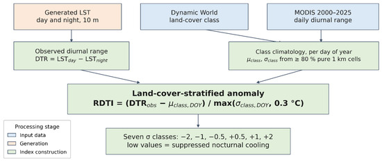
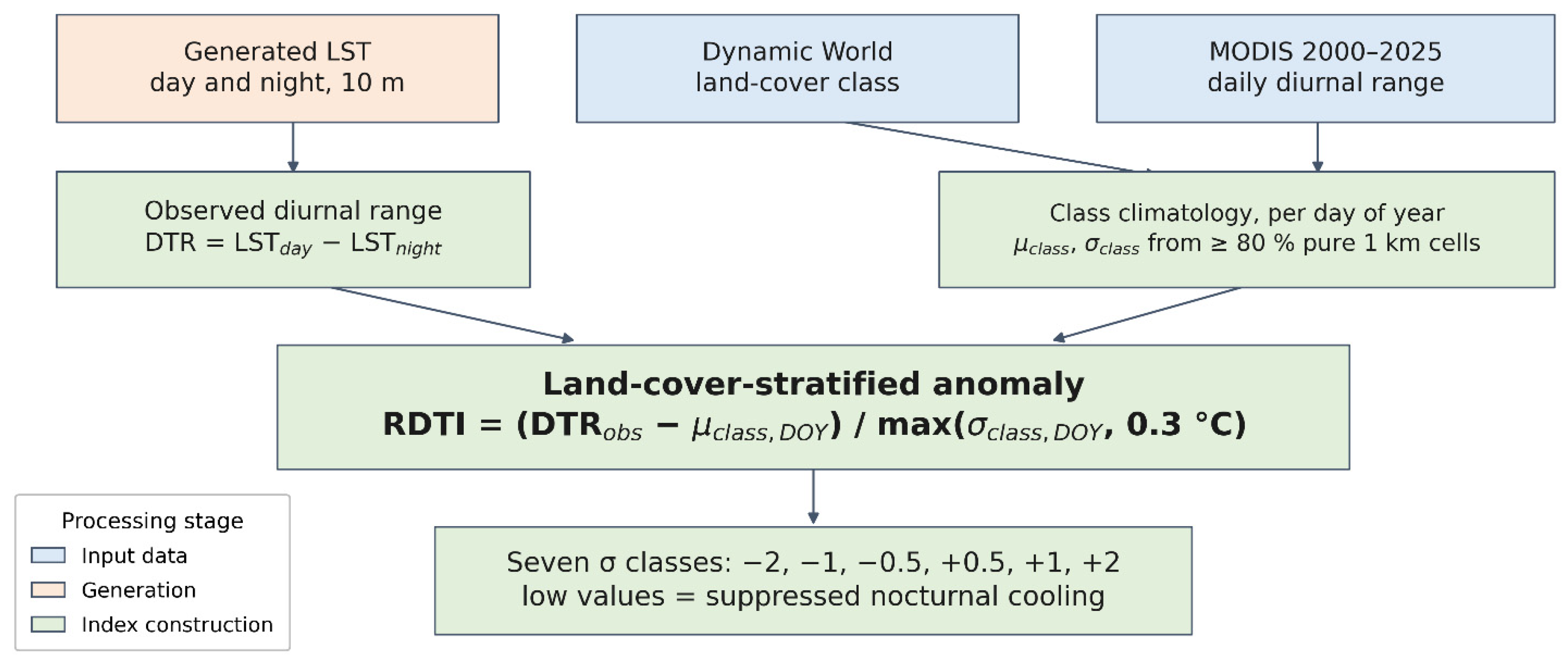
The index rests on three conceptual principles (Figure 4): cooling effectiveness is event-contingent rather than static [27]; it is spatially heterogeneous at the field scale [28]; and it must be judged against the historical behavior of the surface type in question rather than against a scene-wide mean [7].
Figure 4.
Index construction. The observed diurnal temperature range at 10 m is normalized against the mean and standard deviation of the 25-year MODIS record for the pixel’s own land-cover class and day of year, and the resulting anomaly is assigned to seven σ classes. Low values indicate suppressed nocturnal cooling.
The RDTI is applied uniformly across all valid acquisition dates, capturing the full seasonal and inter-annual variability of peri-urban thermal dynamics without dependence on any event-detection threshold. The index operates on a deliberate two-scale architecture.
- The climatological baseline is derived at 1 km resolution from the full 25-year MODIS record (2000–2025), providing the temporal depth that only a long observational record can supply.
- The spatial discrimination is delivered at 10 m from the cGAN-derived LST stack, resolving individual crop parcels and built-up patches.
These two scales are complementary by design: the 1 km climatology anchors each pixel’s thermal anomaly in its long-term norm, while the 10 m spatial component captures the fine-scale heterogeneity that zone-level or coarse-resolution approaches cannot resolve.
For every pixel in the 1 km MODIS product, the daily diurnal temperature range is first computed across the full 2000–2025 record:
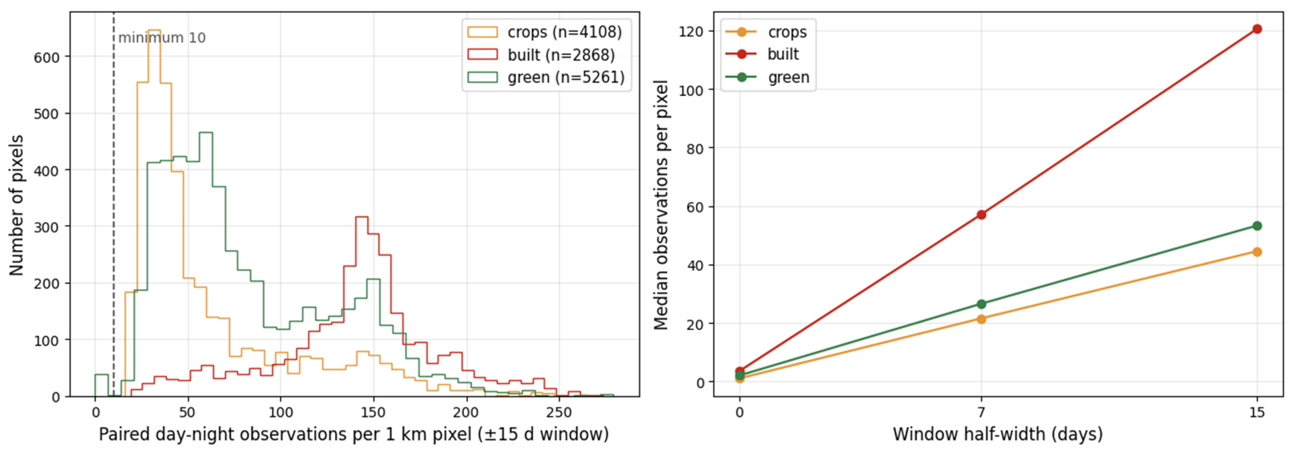
For each pixel and day-of-year, the long-term mean and standard deviation are then derived over a ±15-day window centered on the day of year, providing robust estimates despite cloud contamination. The window width is not arbitrary: a single day of year across 2000–2025 supplies at most 23–24 candidate dates before cloud screening, and after screening the median falls to 1–4 paired day–night observations per 1 km pixel, leaving 90–100% of pixels below any usable minimum. The ±15-day window raises the median to 31–146 paired observations per pixel, with 0–1% of pixels below the minimum observation threshold of 10. Statistics are computed over every date in the record carrying valid retrievals in both the daytime MOD11A1 and the nighttime MYD11A1 product, since the diurnal range cannot be formed from a single overpass; retrievals flagged by the mandatory quality assessment as good quality or other quality are retained, as restricting to good quality alone removes almost all nighttime observations. The resulting climatological surfaces (μ_clim, σ_clim) are computed once at 1 km and stored as DOY-indexed tables (Figure 5).
Figure 5.
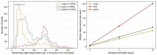
Observations behind the climatological statistics. (Left): distribution of the number of paired daytime and nighttime MODIS observations contributing to each 1 km pixel, by land-cover stratum, for the ±15-day window; the dashed line marks the minimum-observation threshold. (Right): median count against window half-width, showing that a per-day-of-year statistic cannot support the climatology whereas the ±15-day window can.
To account for the distinct thermal regimes of different surfaces, these statistics are computed separately for three land-cover strata derived from a multi-year modal Dynamic World composite [29]: cropland (Dynamic World “crops”), green (trees, grass, flooded vegetation, and shrub/scrub), and built (built-up, together with the small bare and snow/ice fractions, which share the low-evapotranspiration, high diurnal-range thermal behavior of built surfaces). Water was excluded entirely from the stratification and from the index: linear water bodies (the Seine, Deûle, Loire, and Garonne) rarely fill 80% of a 1 km MODIS cell and therefore cannot support a stable, spatially pure climatological stratum. Water accounts for 1.87% (Paris), 0.68% (Lille), 4.26% (Nantes), and 2.72% (Bordeaux) of study-area pixels and appears as masked gaps in all outputs.
Only 1 km cells that were at least 80% pure in a given class (a purity threshold assessed by two-stage aggregation of the 10 m land-cover raster to the 1 km MODIS grid) contributed to that class’s climatology, ensuring each class’s statistics reflect a thermally homogeneous surface. This requirement is restrictive and its cost in coverage is stated explicitly: the proportion of 1 km cells meeting it ranges from 1.1% (vegetated land in Lille) to 39.1% (built-up land in Paris), so class-specific statistics exist only over these fractions of each domain and the index is undefined elsewhere. The resulting per-class, per-DOY statistics were stored as a compact table and applied as class-specific constants to the 10 m diurnal range field within each land-cover mask. No spatial interpolation of the climatological surfaces to 10 m is performed: the baseline contributes a reference level per land-cover class, while all spatial discrimination in the index derives from the 10 m observed diurnal range. A minimum σclim floor of 0.3 °C was imposed to prevent division instability in rare low-variance strata.
The RDTI is defined as the land-cover-stratified climatological anomaly:
DTRobs is the observed diurnal temperature range on the acquisition date, computed from the cGAN-derived 10 m LST stack, and μclass(DOY) and σclass(DOY) are the climatological mean and standard deviation of the daily diurnal range for that pixel’s land-cover class and day-of-year window. The index therefore quantifies how anomalous the observed diurnal range is relative to the pixel-specific, land-cover-stratified seasonal climatology. On each operational date, the observed diurnal temperature range is computed from the GAN-derived 10 m LST stack:
Positive RDTI values indicate stronger nocturnal cooling than the long-term seasonal norm for that land-cover type. Negative values indicate suppressed cooling and heat retention. Pixels belonging to the excluded water class carry no climatology and are masked from the index, as are pixels in 1 km cells that do not meet the 80% purity requirement.
The RDTI is classified into seven interpretability categories (Table 2). As the index is computed relative to a land-cover-stratified, pixel-specific baseline, the classification scheme is statistically self-calibrating: the ±1σ/±2σ/±3σ boundaries are derived from the distribution of RDTI values within each land-cover stratum, rather than from a single domain-wide distribution. This ensures that a given class represents a comparable relative departure from local thermal norms regardless of city or land-cover type.
Table 2.
Seven classification categories of RDTI.
The stratified design adapts automatically to local thermal regimes. The assumption of approximate normality in the underlying distributions was examined directly (Section 3.4): central-class occupancy closely matched the Gaussian expectation, but the distributions were found to be platykurtic, which compresses the intermediate classes and under-populates the extremes. A quantile-based reformulation is therefore recommended for operational deployment and is discussed in Section 4.
This two-scale framework directly addresses the temporal and spatial limitations of the three benchmark methods: it delivers field-scale diurnal LST dynamics grounded in a 25-year climatological record, and a physically interpretable thermal index stratified by land-cover type, applicable to urban heat-adaptation planning and to the surrounding peri-urban landscape.
3. Results
This section reports the results in five parts: (Section 3.1) the 10 m LST inputs generated by the cGAN and their validation against same-date Landsat, against downscaling baselines and against ECOSTRESS; (Section 3.2) the descriptive statistics, spatial structure and thermal classification of the RDTI; (Section 3.3) the land-cover separation achieved by the index; (Section 3.4) the comparison against three established UHI-characterization methods; and (Section 3.5) the propagation of downscaling error into the index and its sensitivity to the water mask.
3.1. Generation and Validation of 10 m LST
Daily 10 m LST was produced for each city and date by a cGAN adapted from the FuseTen architecture [20]. The model was trained per mode (day, night), comparing the 10 m output against Landsat LST. Validation was performed at the target date t2 by resampling the generated 10 m LST to 30 m and comparing against the same-date Landsat acquisition (Table 3, Figure 6).
Table 3.
Validation of the generated 10 m LST at t2 against the same-date Landsat acquisition, computed at 30 m within the study polygon (day mode). Bias and centered RMSE are reported separately and given in °C; r is dimensionless; SD ratio is the ratio of generated to reference standard deviation. Bicubic and bilinear interpolation of the coarse input give centered RMSE of 3.18–3.36 °C for comparison.
Figure 6.
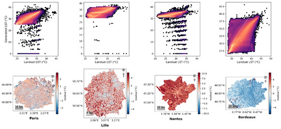
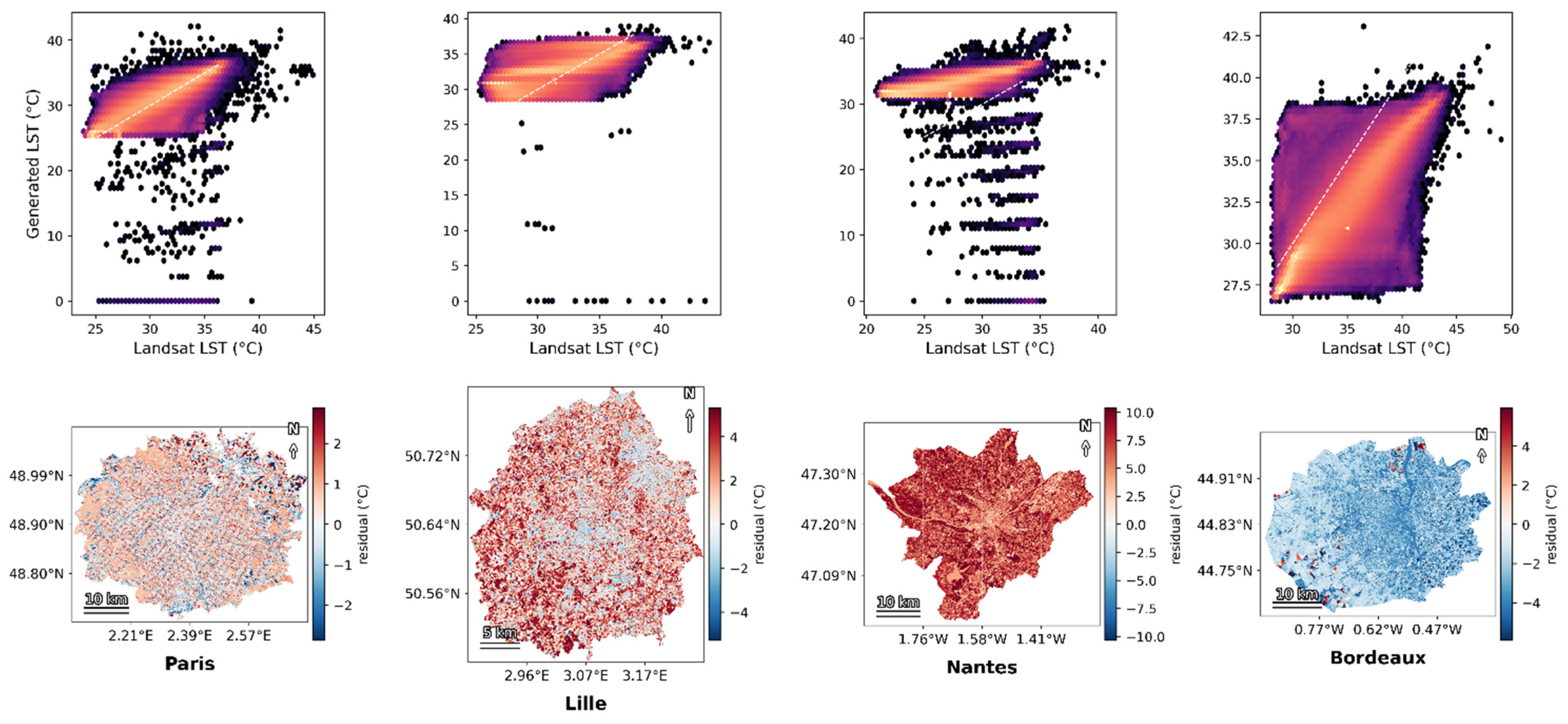
Validation against same-date Landsat observations at t2. (Upper row) Density scatter per city, with bias, centered RMSE and correlation annotated. (Lower row) Spatial distribution of the residual.
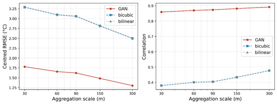
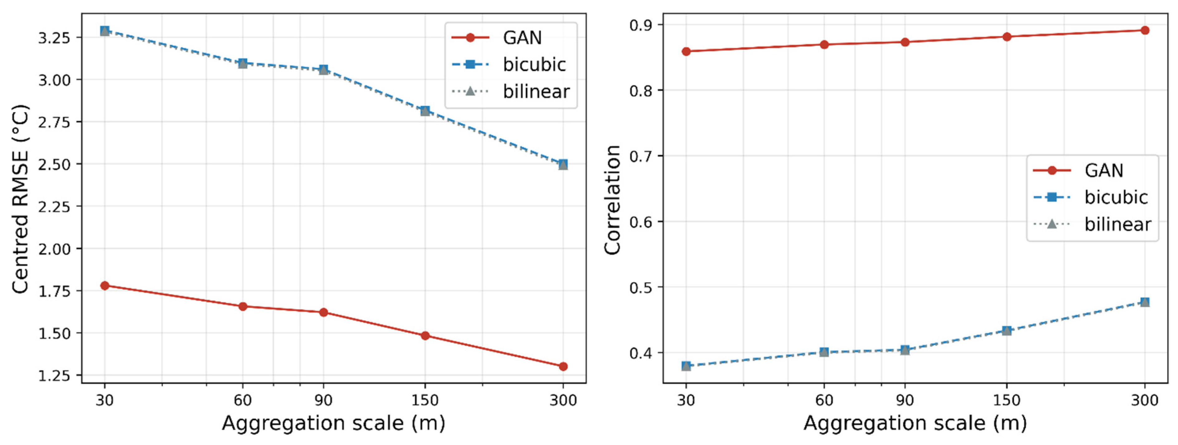
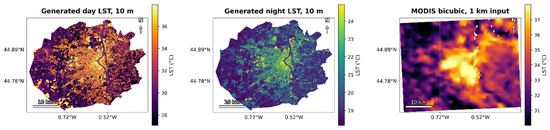
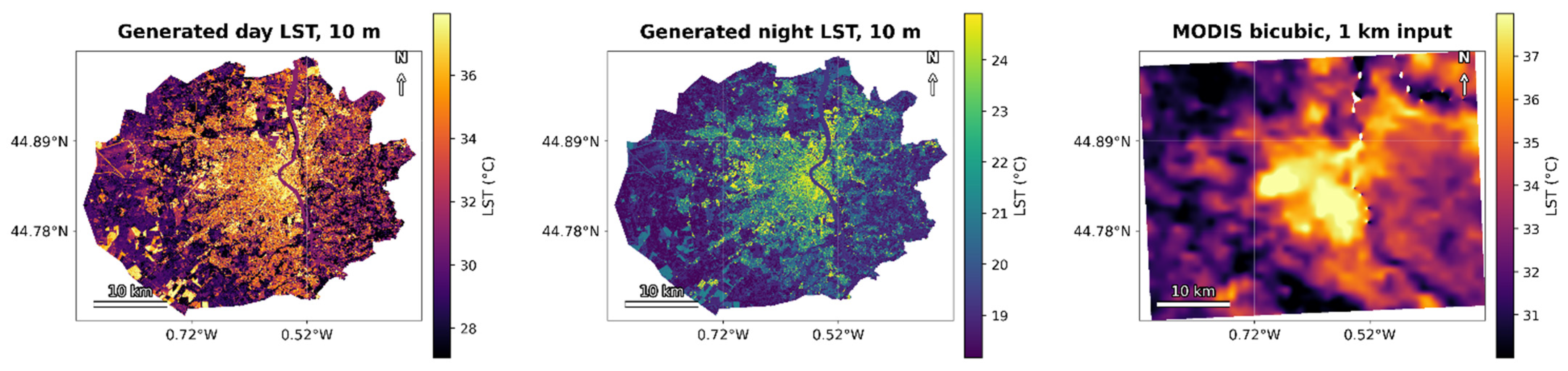
Agreement with the Landsat reference was evaluated at aggregation scales of 30, 60, 90, 150 and 300 m, with every method scored on identical pixels. Bias and centered RMSE are reported separately, because three of the four cities carry a systematic offset against the Landsat reference that is not model error. Centered RMSE at 30 m was 1.03 °C (Paris), 1.54 °C (Bordeaux), 2.13 °C (Lille) and 2.38 °C (Nantes), with correlations of 0.955, 0.920, 0.791 and 0.783, respectively. The corresponding numbers for bicubic and bilinear interpolation of the coarse input are 3.18–3.36 °C and 0.27–0.59 (Figure 7); a visual example can be found in Figure 8. The ratio between the two is stable across the scale range, so the advantage is not an artefact of aggregation and does not erode as resolution increases. Accuracy at 10 m is therefore inferred from this behavior rather than directly measured, and the text states this explicitly.
Figure 7.
Centered RMSE (left) and correlation (right) against the Landsat reference as a function of aggregation scale, averaged over the four study areas, for the generated field and for bicubic and bilinear interpolation of the coarse input. The ratio between methods is stable across the scale range.
Figure 8.
Generated day and night land surface temperature fields at 10 m compared against bicubic interpolation of the 1 km MODIS input.
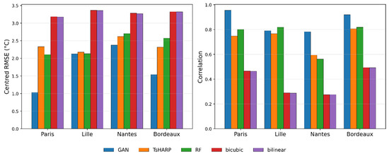
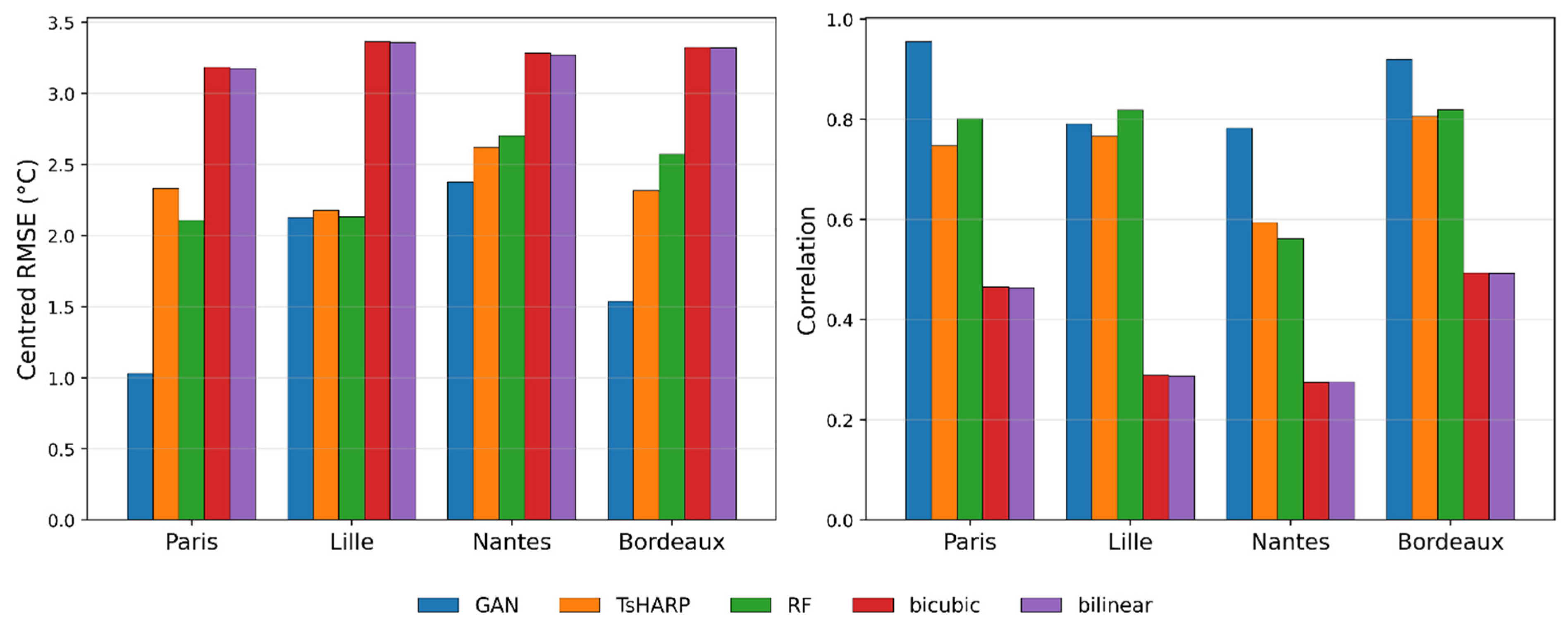
The cGAN was additionally compared against two downscaling baselines that do generate fine-scale detail (Table 4, Figure 9), TsHARP and random-forest downscaling, implemented on the same data, date and grid. Centered RMSE at 30 m was for the cGAN against TsHARP and random forest, respectively: Paris 1.03 against 2.33 and 2.11; Bordeaux 1.54 against 2.31 and 2.57; Lille 2.13 against 2.18 and 2.13; and Nantes 2.38 against 2.62 and 2.70. In Lille the cGAN and the random forest are equivalent, and the random forest attains higher correlation (0.818 against 0.791); this is reported as found. The fields generated are also consistently under-dispersed relative to the reference, with standard deviation ratios of 0.94, 0.83, 0.65 and 0.40 across the four cities.
Table 4.
Comparison of downscaling methods at t2 (30 m): centered RMSE in °C for the conditional GAN, TsHARP and random-forest downscaling. Bias is removed so that the comparison is not dominated by the reference-data offsets. In Lille the cGAN and the random forest are equivalent and the random forest attains the higher correlation.
Figure 9.
Centered RMSE (left) and correlation (right) at 30 m for each downscaling method and city. Bias is removed so that the comparison is not dominated by the reference-data offsets discussed in Section 4.4.
The nighttime field was validated independently against ECOSTRESS L2T_LSTE observations at 70 m. A systematic search returned five usable nighttime overpasses coincident with generated dates, three over Bordeaux and two over Nantes. Because ECOTRESS overpass times differ from the nominal 01:30 local MODIS Aqua sampling time by −2.4 to +3.8 h, surfaces sampled by the two instruments lie at different points on the nocturnal cooling curve; bias therefore absorbs this offset and only centered statistics are directly comparable. Centered RMSE was 0.283–0.437 °C with correlations of 0.903–0.941. Decisively, the built-minus-cropland contrast observed by ECOSTRESS ranged from 0.85 to 1.74 °C across the five nights and was reproduced to within 0.052 °C in every case, so the generated nighttime field reproduces not only the mean level but the night to night variation of the class contrast on which the index is built. A temporal closure test, comparing the generated field aggregated to 1 km against MYD11A1 on acquisition dates the model was not conditioned on, gave RMSE of 1.78–3.15 °C; this establishes independence in time, not in resolution.
3.2. RDTI: Descriptive Statistics, Spatial Structure, and Classification
The RDTI is the climatological anomaly computed against a 25-year (2000–2025) MODIS climatology stratified by land-cover class over a ±15-day day-of-year window. Table 5 reports the per-class and whole-domain descriptive statistics.
Table 5.
RDTI descriptive statistics by land-cover class and whole domain (“all”), within the study area.
The 25-year climatology yields a mean DTR for built surfaces that exceeds that of crops in all four cities. Expressed as the class-normalized anomaly, built DTR is therefore suppressed more strongly than crops DTR in every city. This is the urban heat-retention signature stated in the index’s own terms, in contrast to the raw DTR ordering which reverses between cities, and it is the origin of the crops/built separation. Because the index is a standardized anomaly against a class-specific climatology, the whole-domain mean reflects how each acquisition window compared with that city’s own long-term norm rather than an absolute inter-city temperature difference.
RDTI fields are spatially coherent rather than noisy. A neighborhood-coherence proxy (Pearson correlation between each pixel and its 7 × 7 neighborhood mean, the center pixel excluded) is 0.644 (Paris), 0.769 (Lille), 0.720 (Nantes) and 0.670 (Bordeaux), indicating strong positive spatial autocorrelation. RDTI also tracks built-up intensity continuously: its correlation with NDBI is 0.468 (Paris), 0.531 (Lille) and 0.525 (Bordeaux), and a weaker 0.132 in Nantes, the low value again consistent with that city’s softer built-up thermal contrast. Correlations with distance-to-built are weak and inconsistent (Paris −0.106, Lille +0.089, Nantes −0.035, Bordeaux +0.133), indicating that RDTI does not encode a simple monotonic cooling gradient away from built-up areas (a deliberately reported null result).
Classifying each pixel by its RDTI relative to the per-class mean ± 1/2/3σ thresholds yields the seven-category distribution in Table 6. Central-class (±1σ) occupancy is 61.8–68.4%, close to the Gaussian expectation of 68.3%, supporting approximate normality of the per-class distributions. The extreme-retention classes (1–2) are systematically under-populated; however, class 3 is over-populated, reflecting platykurtic distributions: broad shoulders and thin extreme tails compress genuine variation into the class-3/5 shoulders. A quantile-based classification is therefore a reasonable alternative; the σ-based scheme is retained here for interpretability and comparability with the class definitions.
Table 6.
Percentage of valid pixels in each RDTI class, by city. The Gaussian-expected row is the exact normal-distribution occupancy for the ±kσ thresholds.
3.3. Land-Cover Separation
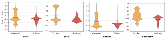
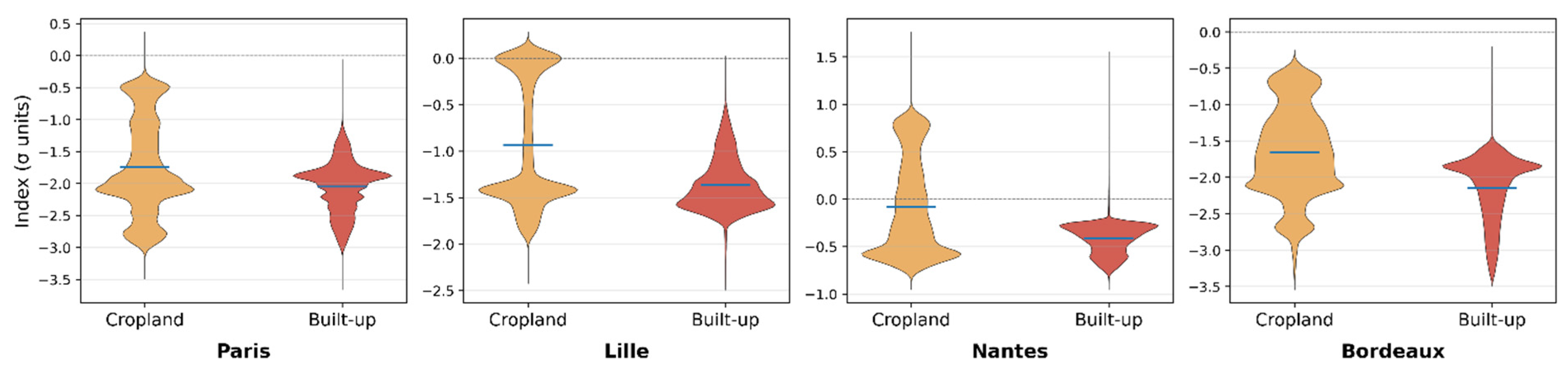
The ability of RDTI to distinguish built from cropland surfaces was quantified from the class distributions over all valid pixels (Table 7, Figure 10). The separation is negative in every city, indicating that built-up surfaces carry a lower index than cropland and therefore cool less strongly overnight relative to their own class norm. The effect is largest in Nantes (Cohen’s d 1.67) and Bordeaux (1.59), and smallest in Paris (0.54), where cropland occupies a much smaller share of the domain than built-up land (578,554 against 2,463,364 valid pixels). Effect size is reported in preference to a significance test: with class samples in the hundreds of thousands and strong spatial autocorrelation between neighboring pixels, a p-value would be inflated by pseudo-replication, whereas Cohen’s d is scale-free and unaffected by sample size.
Table 7.
Two-sample KS test of RDTI, built versus crops, per city. Separation is the difference of class means (crops−built).
Figure 10.
Distribution of the index over cropland and built-up land for each study area. Lower values indicate suppressed nocturnal cooling. The blue line indicates the median value for each land cover class.
3.4. Comparison with Established UHI-Characterization Methods
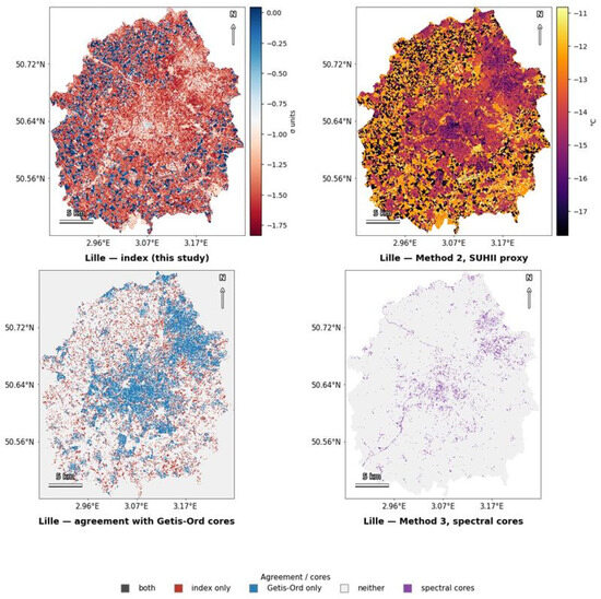
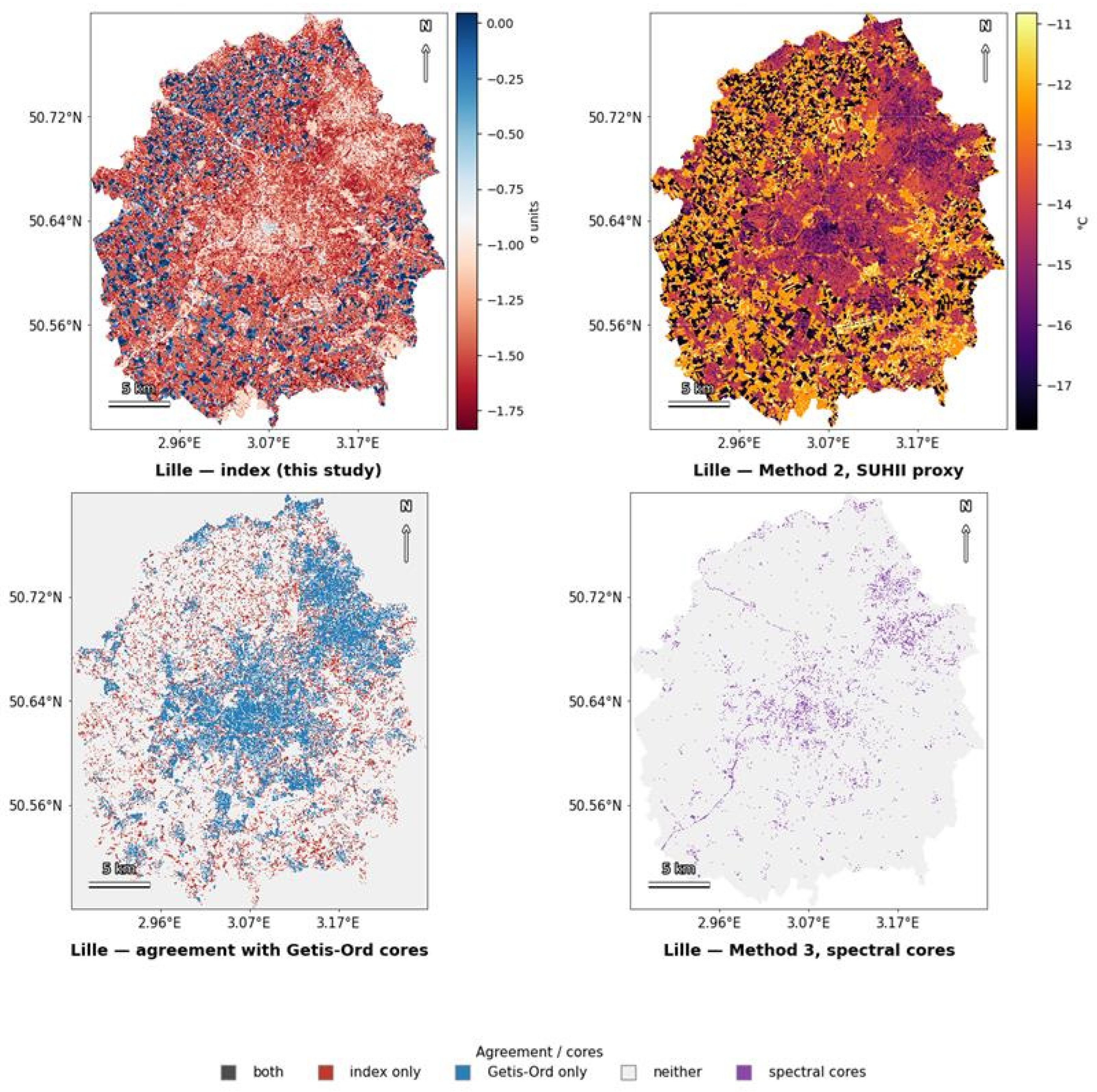
RDTI heat-retention pixels (classes 1–3) were compared against three reference methods computed on the same 10 m LST stack (Table 8, Figure 11). Agreement is quantified with Cohen’s κ rather than raw percentage agreement, because RDTI flags only 16–21% of pixels and a null classifier flagging nothing would spuriously “agree” on 79–84% of pixels which is exactly the raw-agreement range obtained with the original binary flags. For Method 2, whose native anomaly surface is almost entirely negative, a relative hot-spot flag rate-matched to RDTI (top quintile/top decile of the SUHII proxy) is used; Methods 1 and 3 use their published binary core flags, whose near-zero firing rates produced the misleadingly high raw agreement.
Table 8.
Cohen’s κ between RDTI heat-retention (classes 1–3) and each reference method. Method 2 is shown for two rate-matched thresholds (top 20% and top 10% of the SUHII proxy). Positive κ indicates agreement beyond chance; values near zero indicate statistical independence.
Figure 11.
Spatial comparison of urban heat island characterization methods for one study area. From left: the index of this study; the Method 2 SUHII proxy; the agreement map against Method 1 Getis–Ord persistent cores, distinguishing pixels flagged by both methods, by the index only, by the reference method only, and by neither; and the Method 3 spectral cores.
RDTI correlates at −0.664 (Paris), −0.798 (Lille), −0.291 (Nantes) and −0.799 (Bordeaux) with the rate-matched SUHII proxy. The negative sign is the expected relationship and not a disagreement: suppressed nocturnal cooling produces a smaller diurnal range, and hence a lower index value, in the same locations where SUHII reports a positive temperature excess. Because this statistic is threshold-free it requires no prevalence matching. Expressed categorically at matched prevalence, Cohen’s κ against the SUHII proxy is 0.414, 0.349, 0.158 and 0.477, while agreement with the two absolute hot-spot delineations is near zero to negative (Getis–Ord G* cores −0.352 to −0.122; spectral cores −0.041 to −0.011). Where the index flags retention that the Getis–Ord delineation does not, that area is predominantly cropland in Lille and Nantes (37% and 45%) but not in Paris or Bordeaux (12% and 5%), so the divergence is not uniformly attributable to agricultural land.
3.5. Uncertainty Propagation and Sensitivity to the Water Mask
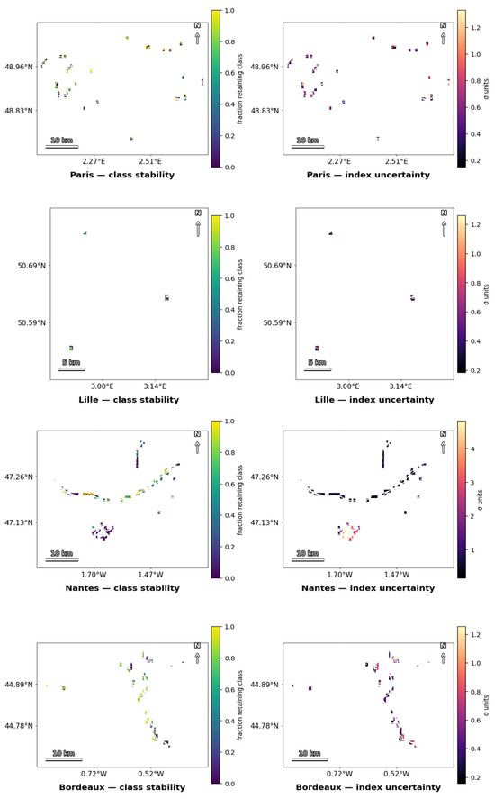
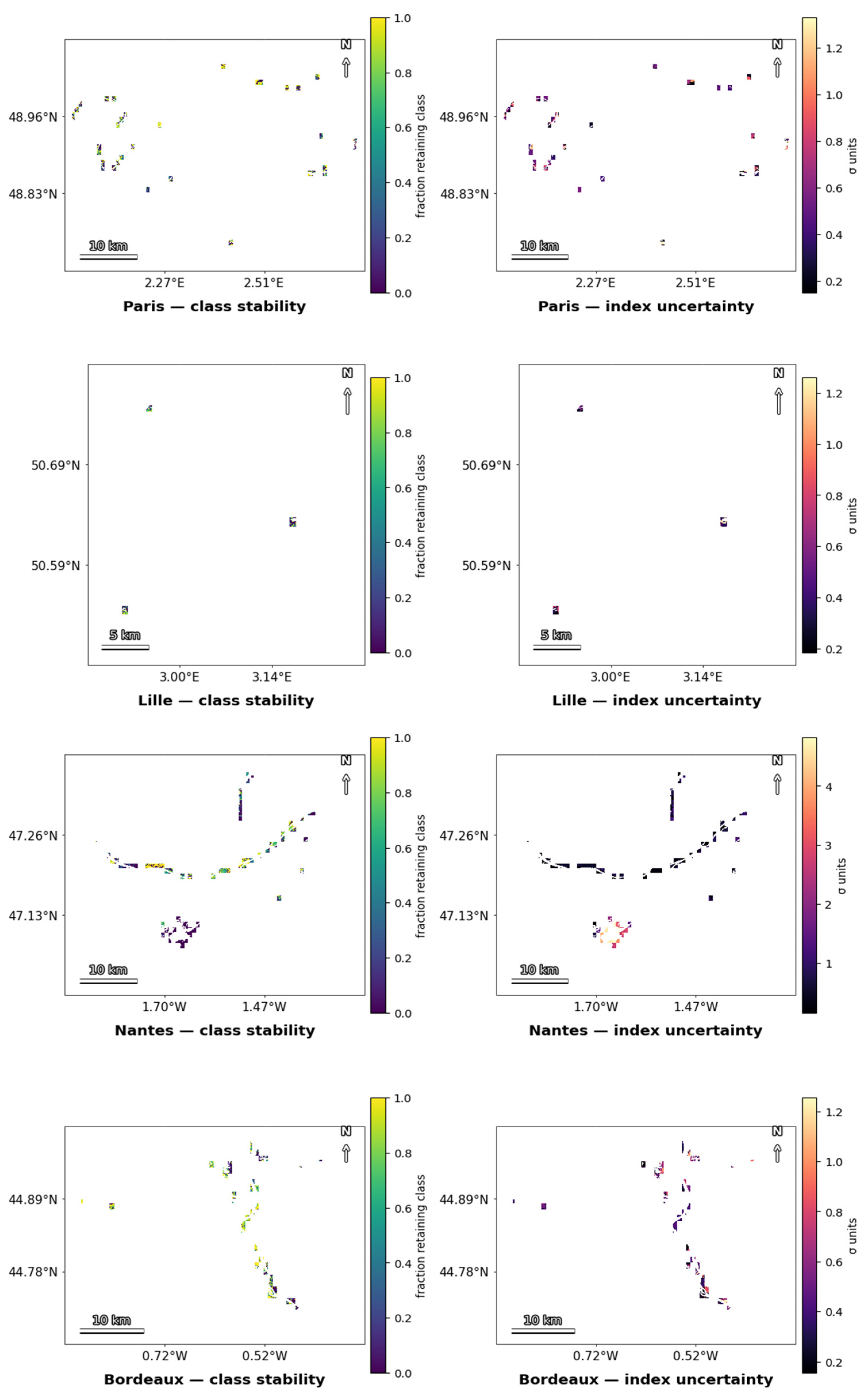
The propagation of downscaling error into the index was quantified by Monte Carlo simulation (Figure 12). Thirty perturbed realizations of the generated day and night fields were produced per city, with spatially correlated noise whose amplitude was set from the per-city validated residual standard deviation (0.61–0.74 °C) and whose correlation length and nugget fraction were estimated by fitting an exponential variogram to the validation residuals (range 165–336 m, nugget fraction 0.26–0.31). Each realization was propagated through the full index. Mean per-pixel index uncertainty was 0.50–1.13 σ units. Because the seven classes are 0.5σ wide, an uncertainty of this magnitude spans most of one band, so reassignment to an adjacent class is arithmetically expected and an exact agreement figure understates stability. Because the index is computed from the day-minus-night difference and expressed as a standardized anomaly against a class-specific climatology, spatially coherent errors of common sign in the two input fields largely cancel in the difference and any residual constant offset is absorbed by the normalization.
Figure 12.
Propagation of downscaling error into the index. (Upper row) Fraction of Monte Carlo realizations in which each pixel retains its seven-class assignment. (Lower row) Per-pixel index standard deviation, in σ units. Noise was spatially correlated with the amplitude, correlation length and nugget fraction measured from the validation residuals.
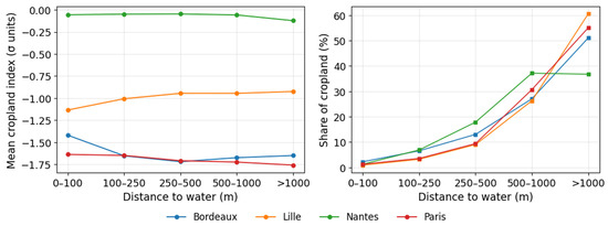
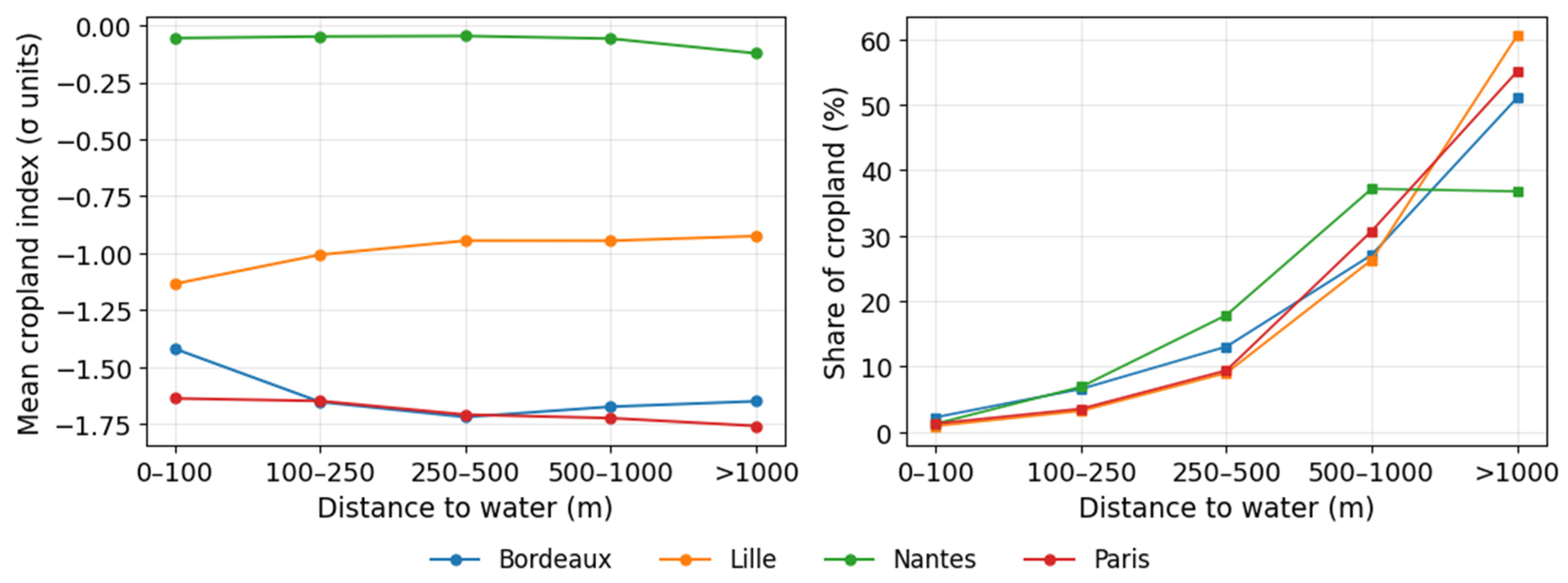
The exclusion of water pixels from the stratification was tested directly by stratifying cropland by distance to the nearest water body (Figure 13). Between 13.2% and 26.1% of cropland lies within 500 m of water. Comparing the 0–100 m stratum with cropland beyond 1000 m gives differences of +0.121 (Paris), −0.210 (Lille), +0.067 (Nantes) and +0.230 (Bordeaux) index units. The sign is not consistent across cities: only in Lille does near-water cropland show the additional cooling that exclusion of water pixels might be expected to conceal, while in the other three the relationship is reversed. Against a built-versus-cropland separation of Cohen’s d = 0.54–1.67, the implied bias is therefore bounded and not systematic.
Figure 13.
Mean cropland index by distance to the nearest water body (left) and the share of cropland in each distance band (right), for the four study areas.
4. Discussion
4.1. Generation of Field-Scale Diurnal LST
The cGAN produced 10 m LST fields that were validated against same-date Landsat with centered RMSE between 1.03 and 2.38 °C and correlation between 0.78 and 0.96 across the four cities at 30 m, with bias reported separately because three of the four cities carry a systematic offset against the Landsat reference that is not model error (Section 4.4). These figures fall within the performance envelope reported for the FuseTen/weakly-supervised generative lineage on which the architecture is based [20], confirming that a non-linear generative fusion of thermal and optical sources can reconstruct field-scale surface temperature at accuracies comparable to the source Landsat product itself.
More important than the absolute error is the comparison against methods that also generate fine-scale detail. Against interpolation of the coarse conditioning input the margin is large, centered RMSE of 1.03–2.38 °C versus 3.18–3.36 °C, but interpolation produces no fine-scale structure by construction and outperforming it therefore establishes little. Against TsHARP and random-forest downscaling, which do, the cGAN retains an advantage in three of four cities, while in Lille it is equivalent to the random forest. This is the evidence that the generated fields are not smoothed reproductions of the MODIS signal but genuinely incorporate the fine-scale spatial information carried by the Sentinel-2 and Landsat encoder branches, on which the two-scale architecture depends.
The bias term deserves comment as it bears on the index. Bias was small and, critically, showed no systematic direction across cities (−1.16 to +1.04 °C; slightly cold in Paris, Lille and Nantes, slightly warm in Bordeaux). Because RDTI is built on the diurnal difference between day and night LST, a spatially uniform bias of the same sign in both fields would cancel in the difference; and because the index is expressed as a standardized anomaly against a class-specific climatology, a residual constant offset is further absorbed into the normalization. The index is therefore structurally more robust to the modest calibration offsets that remain in the generated fields than an absolute-temperature product would be (a property that follows directly from its anomaly-based formulation).
Performance was not uniform. Nantes was the weakest city on several axes: the largest centered RMSE among the four (2.38 °C), the weakest coupling to built-up intensity (NDBI correlation 0.132 against 0.47–0.53 elsewhere), the weakest correlation with the SUHII proxy (−0.291 against −0.66 to −0.80 elsewhere), and the lowest dispersion ratio (0.40). Part of this pattern reflects a reference-data problem rather than model failure: in Nantes the generated field agrees with MODIS to within 0.23 °C while differing from the Landsat reference by 6.8 °C, which locates the discrepancy in the reference (Section 4.4). The remainder is consistent with an acquisition window sampling a landscape of genuinely lower thermal contrast, in which the built/rural signal that the model and the index both exploit was simply weaker.
4.2. RDTI and the Climatological Reframing of the Diurnal Signal
The central conceptual result of this study concerns how the DTR should be interpreted once it is normalized against a land-cover-stratified climatology. In absolute terms, the raw DTR ordering between built and agricultural surfaces was inconsistent across the four cities: built surfaces showed a larger diurnal range than cropland in three cities but a marginally smaller one in Bordeaux. Taken at face value, this inconsistency would undermine any claim that the index captures a stable urban thermal signature.
The resolution comes from the climatology itself. The 25-year MODIS baseline shows that built surfaces have a higher mean DTR than cropland in all four cities. When each observation is expressed as a departure from its own class-specific norm, the picture becomes clear: built-up DTR is suppressed more strongly than cropland DTR relative to climatology in every city. This is the urban heat-retention signature (built surfaces failing to achieve their expected nocturnal cooling) stated in the index’s own terms, and it holds without exception where the raw ordering did not. This is precisely the advantage the introduction anticipated for a land-cover-stratified anomaly over a land-cover-blind average [6]: the stratification does not merely refine the signal, it reverses an apparent contradiction into a consistent one.
A consequence is that whole-city mean RDTI must not be read as an absolute intercity temperature comparison. This revised manuscript distinguishes explicitly between two classes of result: within-city, land-cover-relative quantities, which are comparable across cities because each is computed against that city’s own stratified baseline; and domain-mean index values, which encode the thermal character of each city’s acquisition window relative to its own 25-year norm and must not be read as intercity temperature comparisons. Three cities (Paris, Lille, Bordeaux) sampled windows in which the diurnal range was suppressed relative to their own norms, a signature consistent with heatwave conditions in which elevated nighttime minima compress the day/night contrast [8,9]; Nantes sampled a near-normal window.
The single positive class anomaly in this study is instructive. Nantes green space was the only class/city combination with an observed DTR above its climatological norm, and it carried the highest class-mean RDTI in this study. Under the index’s construction, this means Nantes vegetation cooled more strongly than its 25-year baseline during the observation window, the active vegetative cooling response that the introduction identifies as a feature of the peri-urban thermal system [6]. That it appears as a positive anomaly rather than an absolute temperature minimum illustrates the interpretive shift the index requires: green space scored against green’s own norm reveals functioning, whereas green scored against a domain-wide mean would simply appear cool.
4.3. Relationship to Established UHI-Characterization Methods
The cross-method comparison produced a result that is initially counter-intuitive but, on inspection, validates the index’s construct. The index correlates at −0.291 to −0.799 with the rate-matched SUHII proxy, the negative sign being the expected relationship rather than a disagreement, since suppressed nocturnal cooling produces a smaller diurnal range and hence a lower index value where SUHII reports a positive temperature excess. Expressed categorically at matched prevalence, Cohen’s κ against the SUHII proxy is 0.158–0.477, while agreement with the two absolute-temperature methods is near zero to negative (Getis–Ord G* cores −0.352 to −0.122; spectral cores −0.041 to −0.011). The index therefore aligns with a continuous measure of relative thermal excess and is systematically distinct from methods that identify absolute temperature maxima, which is precisely the behavior its construction predicts.
4.4. Strengths and Limitations
The principal strengths of the approach follow from its design. First, the two-scale architecture couples the temporal depth of a multi-decade 1 km climatology with the spatial detail of a 10 m generative reconstruction, and the baseline comparison confirms the 10 m layer contributes genuine fine-scale information rather than a resampled MODIS signal. Second, the land-cover-stratified anomaly formulation resolves an otherwise inconsistent raw diurnal signal into a consistent heat-retention signature (Section 4.2). Third, the index is single-term and therefore carries no free parameters: there is no weighting scheme to calibrate and correspondingly no scope for overfitting. Fourth, the resulting fields are spatially coherent, with neighborhood coherence of 0.92–0.97, and the nighttime field on which the index depends is validated against an independent sensor at 70 m.
Several limitations bound the interpretation of these results. First, variance preservation: the generated fields are consistently under-dispersed relative to the Landsat reference, with standard-deviation ratios of 0.94, 0.83, 0.65 and 0.40 across the four cities, and in Lille and Nantes TsHARP preserved variance better. This is the opposite of the failure mode usually associated with adversarial downscaling, in which fine-scale texture is fabricated; the present model is conservative rather than hallucinatory, which is the safer direction for an index built on anomalies, but it will attenuate extreme values. Second, reference-data disagreement: MODIS and Landsat daytime observations of the same date differ by 0.4, 2.3, 3.4 and 6.6 °C across Bordeaux, Lille, Paris and Nantes, as estimated independently from the TsHARP residual and from aggregation of the generated field to 1 km. In Nantes the generated field agrees with MODIS to within 0.23 °C while differing from the Landsat reference by 6.8 °C, which locates the discrepancy in the reference rather than in the model; validation statistics for Nantes should be read with this in mind. Third, coverage: because a class-specific climatology exists only where a 1 km cell is at least 80% pure, the index is defined over 1.1–39.1% of each domain depending on class and city. Fourth, classification stability: under Monte Carlo perturbation at the measured error magnitude, mean per-pixel index uncertainty is 0.50–1.13 σ units; because the classes are 0.5σ wide, reassignment to an adjacent class is arithmetically expected, which supports the quantile-based reformulation recommended. The seven-class scheme also assumes approximate normality that the data only partly satisfy: the distributions are platykurtic, so intermediate classes are over-populated and the extreme retention classes nearly empty [7,30,31]. Finally, the cGAN was validated against same-date Landsat at 30 m and against ECOSTRESS at 70 m, but no in situ LST validation was available; Météo-France station networks provide air temperature, which is not the same physical quantity and cannot serve as validation for an LST product.
5. Conclusions
This study sets out to test whether generative fusion could deliver field-scale diurnal LST in heterogeneous peri-urban landscapes, and whether an index built on that LST could describe nocturnal thermal behavior in terms that existing coarse, daytime, or land-cover-blind UHI indicators cannot. Both objectives are met, though with different degrees of confidence, and it is worth stating plainly where the evidence is firm and where it is not.
The first hypothesis holds: the cGAN reconstructs field-scale diurnal LST that carries genuine 10 m structure rather than a resampled coarse signal, and it does so consistently across four independent metropolitan settings. The second hypothesis holds in the terms in which it is now stated. The index captures nocturnal, field-scale, land-cover-relative thermal structure. It separates built from cropland surfaces in every city, correlates with relative-warmth methods while remaining distinct from absolute hot-spot methods, and behaves as its construction predicts.
The most instructive finding is regional rather than methodological. The four cities did not behave alike, and the differences are not noise. Bordeaux showed the strongest built–cropland separation and the strongest urban/rural contrast; Nantes sat at the opposite end on every axis having the weakest model margin over interpolation, weakest coupling to built-up intensity, and a near-neutral domain index; while Paris and Lille fell between. Read together rather than city by city, these are not four unequal validations of one method but a single coherent gradient of thermal contrast: where the urban/rural signal is physically strong, both the model and the index resolve it sharply; where the landscape is genuinely low-contrast, both weaken together. The disparity is therefore a property of the territories, not an instability of the tool. But it also means the index’s discriminatory power is contingent on the thermal contrast available in a given metropole and season, and cross-metropole comparison of absolute index levels is not warranted. This regional contingency is itself the most transferable empirical result of the work.
Two critical reservations bound these conclusions and should frame any use of the index. The first is validity. The daytime accuracy figures are agreement with same-date Landsat rather than validated absolute accuracy, and three of the four cities carry a systematic offset against that reference. The nighttime field is now validated independently against ECOSTRESS at 70 m, which removes the most serious gap in the original submission, but no in situ LST validation was available and absolute index levels remain affected by the compression of the generated diurnal range described in Section 4.4. Until independent in situ validation is carried out, absolute levels should be treated as internally consistent rather than externally confirmed, while class contrasts within a city, which are differences and therefore unaffected by a common offset, can be read with more confidence. The second is reproducibility.
Several perspectives follow directly. Independent validation against in situ observations, prioritizing a nighttime reference, remains the single most important next step and the precondition for treating the accuracy figures as absolute. Resolving the reference data disagreement between MODIS and Landsat, and the associated compression of the generated diurnal range, is a prerequisite for interpreting absolute index levels. A quantile-based reformulation of the seven-class scheme would remove its dependence on an approximate-normality assumption the data only partly support. Pairing the index with field-scale agronomic outcomes across several seasons would extend it toward agricultural application, which is outside the scope of the present study.
Supplementary Materials
The following supporting information can be downloaded at: https://www.mdpi.com/article/10.3390/rs18183259/s1. Table S1. Mean, standard deviation, extremes, and 1st/99th percentiles of the generated 10 m LST (°C), by city and mode, within the study polygon. Table S2. Mean day LST, mean night LST, and mean diurnal temperature range (DTR = day − night) of the observed fields, by land-cover class and city (°C), together with the 25-year climatological mean DTR (μ_clim) and standard deviation (σ_clim) against which each class is normalized. Observed DTR SD is the within-class spatial standard deviation.
Author Contributions
All authors contributed to the study conception and design. Material preparation, data collection and analysis were performed by N.E.B. and M.A.S. The first draft of the manuscript was written by N.E.B. and all authors commented on previous versions of the manuscript. Conceptualization, N.E.B., M.A.S., R.D.S. and R.N.; methodology, N.E.B.; formal analysis, N.E.B.; investigation, N.E.B.; writing—original draft preparation, N.E.B. and M.A.S.; writing—review and editing, N.E.B., M.A.S., R.D.S. and R.N.; supervision, M.A.S., R.D.S. and R.N. All authors have read and agreed to the published version of the manuscript.
Funding
This research received no external funding.
Data Availability Statement
The data and methods used in Google Earth Engine are available in the Supplementary Materials.
Conflicts of Interest
The authors declare no conflicts of interest.
Abbreviations
The following abbreviations are used in this manuscript:
| LST | Land surface temperature |
| MODIS | Moderate Resolution Imaging Spectroradiometer |
| MOD11A1 | MODIS/Terra daily 1 km LST product (daytime) |
| MYD11A1 | MODIS/Aqua daily 1 km LST product (nighttime) |
| GEE | Google Earth Engine |
| GeoTIFF | Geostationary Earth Orbit Tagged Image File Format (georeferenced raster file) |
| NDVI | Normalized Difference Vegetation Index |
| NDWI | Normalized Difference Water Index |
| NDBI | Normalized Difference Built-up Index |
| NIR | Near-infrared (spectral band) |
| SWIR | Short-wave infrared (spectral band) |
| RDTI | Relative Diurnal Thermal Index (this study) |
| DTR | Diurnal temperature range |
| UHI | Urban heat island |
| SUHII | Surface Urban Heat Island Intensity |
| DOY | Day of year |
| GAN | Generative adversarial network |
| cGAN | Conditional generative adversarial network |
| FuseTen | The weakly supervised generative fusion framework the architecture adapts (proper name, not an initialism) |
| AdaIN | Adaptive instance normalization |
| PatchGAN | Patch-based GAN discriminator (proper name) |
| RAM | Random-access memory |
| RMSE | Root mean square error |
| MAE | Mean absolute error |
| SD | Standard deviation |
| SSIM | Structural Similarity Index Measure |
| PSNR | Peak signal-to-noise ratio |
| ERGAS | Erreur Relative Globale Adimensionnelle de Synthèse (Relative Dimensionless Global Error in Synthesis) |
| KS | Kolmogorov–Smirnov (test) |
| t1, t2 | Reference date/target date in the GAN inference pair |
| κ | Cohen’s kappa (chance-corrected agreement) |
| r/R2 | Pearson correlation coefficient/coefficient of determination |
| G* | Getis–Ord Gi* local hot-spot statistic |
References
- Huang, Z.; Duan, L.; Xu, Y.; Yang, S.; Lin, Z.; Yue, H.; Yang, J. Exploring the Influence of Urban Green Space and Urban Morphology on Urban Heat Islands Using Street View and Satellite Imagery. Sci. Rep. 2025, 15, 23759. [Google Scholar] [CrossRef] [Scilit]
- Jeon, M.; Park, K.; Moon, W.; Kim, J.-J.; Baik, J.-J. Exploring Urban Heat Islands with a Simple Thermodynamic Model. Nonlinear Process. Geophys. 2026, 33, 17–32. [Google Scholar] [CrossRef] [Scilit]
- Shi, T.; Yang, Y.; Zong, L.; Guo, M.; Qi, P.; Lolli, S. The Modulation of Synoptic Weather Patterns and Human Activities on the Diurnal Cycle of the Summertime Canopy Urban Heat Island in the Yangtze River Delta Urban Agglomeration, China. Atmos. Chem. Phys. 2025, 25, 4989–5007. [Google Scholar] [CrossRef] [Scilit]
- Zhao, L.; Fan, X.; Hong, T. Urban Heat Island Effect: Remote Sensing Monitoring and Assessment—Methods, Applications, and Future Directions. Atmosphere 2025, 16, 791. [Google Scholar] [CrossRef] [Scilit]
- Liu, L.; Zhang, W. Contrary to Expectation: The Surface Urban Heat Island Intensity Is Increasing in Population Shrinking Region While Decreasing in Population Growing Region-A Comparative Analysis from China. PLoS ONE 2024, 19, e0300635. [Google Scholar] [CrossRef] [Scilit]
- Yan, Z.; Li, W.; Yu, L.; Li, X.; Bu, K.; Liu, H. Intensification or Marginalization: Peri-Urban Agriculture for Mitigating Urban Heat Island Effects in Summer. npj Urban Sustain. 2026, 6, 19. [Google Scholar] [CrossRef] [Scilit]
- Giménez, V.D.; Serrago, R.A.; Kettler, B.; García, G.A.; Impa, S.M.; Krishna Jagadish, S.V.; Prasad, P.V.V.; Miralles, D.J.; Ciampitti, I.A. Nighttime Warming Affects Yields of Major Grain Crops: A Global Meta-Analysis. Field Crops Res. 2025, 334, 110142. [Google Scholar] [CrossRef] [Scilit]
- Strohmenger, L.; Collet, L.; Andréassian, V.; Corre, L.; Rousset, F.; Thirel, G. Köppen–Geiger Climate Classification across France Based on an Ensemble of High-Resolution Climate Projections. Comptes Rendus. Géosci. 2024, 356, 67–82. [Google Scholar] [CrossRef] [Scilit]
- Beobide-Arsuaga, G.; Suarez-Gutierrez, L.; Barkhordarian, A.; Olonscheck, D.; Baehr, J. Increasing Central and Northern European Summer Heatwave Intensity Due to Forced Changes in Internal Variability. Nat. Commun. 2025, 16, 9485. [Google Scholar] [CrossRef] [Scilit]
- Cafaro, R.; Cardone, B.; D’Ambrosio, V.; Di Martino, F.; Miraglia, V. A New GIS-Based Framework to Detect Urban Heat Islands and Its Application on the City of Naples (Italy). Land 2024, 13, 1253. [Google Scholar] [CrossRef] [Scilit]
- Altıner, F.; Bingöl, F. Spatio-Temporal Assessment of Land Surface Temperature, Vegetation Cover, and Built-Up Areas Using LST, NDVI, and NDBI in Balıkesir, Türkiye (1985–2025). Sustainability 2025, 17, 9245. [Google Scholar] [CrossRef] [Scilit]
- Wang, J.; Lu, L.; Zhou, X.; Huang, G.; Chen, Z. Spatio-Temporal Patterns and Drivers of the Urban Heat Island Effect in Arid and Semi-Arid Regions of Northern China. Remote Sens. 2025, 17, 1339. [Google Scholar] [CrossRef] [Scilit]
- Ullah, N.; Siddique, M.A.; Ding, M.; Grigoryan, S.; Zhang, T.; Hu, Y. Spatiotemporal Impact of Urbanization on Urban Heat Island and Urban Thermal Field Variance Index of Tianjin City, China. Buildings 2022, 12, 399. [Google Scholar] [CrossRef] [Scilit]
- Dong, R.; Wurm, M.; Taubenböck, H. Seasonal and Diurnal Variation of Land Surface Temperature Distribution and Its Relation to Land Use/Land Cover Patterns. Int. J. Environ. Res. Public Health 2022, 19, 12738. [Google Scholar] [CrossRef] [Scilit]
- Beck, H.E.; Zimmermann, N.E.; McVicar, T.R.; Vergopolan, N.; Berg, A.; Wood, E.F. Present and Future Köppen-Geiger Climate Classification Maps at 1-Km Resolution. Sci. Data 2018, 5, 180214, Correction in Sci. Data 2020, 7, 274. [Google Scholar] [CrossRef] [Scilit]
- Perrin, C.; Clément, C.; Melot, R.; Nougarèdes, B. Preserving Farmland on the Urban Fringe: A Literature Review on Land Policies in Developed Countries. Land 2020, 9, 223. [Google Scholar] [CrossRef] [Scilit]
- Al-Qubati, A.; Zhang, L.; Forkel, M. Urban and Peri-Urban Agriculture under Climate Change: A Review on Carbon Emissions and Sequestration. Sustain. Cities Soc. 2024, 115, 105830. [Google Scholar] [CrossRef] [Scilit]
- Cimino, O.; Giarè, F.; Henke, R. Periurban Agriculture and Organic Farming: Investigating Synergies and Policy Implications. Land 2025, 14, 690. [Google Scholar] [CrossRef] [Scilit]
- Gorelick, N.; Hancher, M.; Dixon, M.; Ilyushchenko, S.; Thau, D.; Moore, R. Google Earth Engine: Planetary-Scale Geospatial Analysis for Everyone. Remote Sens. Environ. 2017, 202, 18–27. [Google Scholar] [CrossRef] [Scilit]
- Bouaziz, S.; Hafiane, A.; Canals, R.; Nedjai, R. FuseTen: A Generative Model for Daily 10 m Land Surface Temperature Estimation From Spatio-Temporal Satellite Observations. In Proceedings of the 2025 International Conference on Machine Intelligence for GeoAnalytics and Remote Sensing (MIGARS); IEEE: New York, NY, USA, 2025; pp. 1–4. [Google Scholar]
- El Beyrouthy, N.; Al Sayah, M.; Der Sarkissian, R.; Nedjai, R. Enhancing Urban Temperature Monitoring through High-Resolution Remote Sensing and Advanced Data Processing Techniques. Theor. Appl. Climatol. 2025, 156, 396. [Google Scholar] [CrossRef] [Scilit]
- Huang, X.; Belongie, S. Arbitrary Style Transfer in Real-Time with Adaptive Instance Normalization. In Proceedings of the 2017 IEEE International Conference on Computer Vision (ICCV); IEEE: New York, NY, USA, 2017; pp. 1510–1519. [Google Scholar]
- Isola, P.; Zhu, J.-Y.; Zhou, T.; Efros, A.A. Image-to-Image Translation with Conditional Adversarial Networks. In Proceedings of the 2017 IEEE Conference on Computer Vision and Pattern Recognition (CVPR); IEEE: New York, NY, USA, 2017; pp. 5967–5976. [Google Scholar]
- Kara, Y.; Yavuz, V.; Lupo, A.R. Multi-Index Assessment of Surface Urban Heat Island (SUHI) Dynamics in Samsun Using Google Earth Engine. Atmosphere 2025, 16, 712. [Google Scholar] [CrossRef] [Scilit]
- Rao, P.; Tassinari, P.; Torreggiani, D. Exploring the Land-Use Urban Heat Island Nexus under Climate Change Conditions Using Machine Learning Approach: A Spatio-Temporal Analysis of Remotely Sensed Data. Heliyon 2023, 9, e18423. [Google Scholar] [CrossRef] [Scilit]
- Bin Ali, A.A.; Mitra, C.; Rishal, F.H.; Hossain, R. Bin Mapping and Predicting Urban Heat Island Intensity Hotspots through a Space–Time Machine Learning Framework in Bangladesh. Comput. Urban Sci. 2026, 6, 14. [Google Scholar] [CrossRef] [Scilit]
- Zhao, J.; Meili, N.; Zhao, X.; Fatichi, S. Urban Vegetation Cooling Potential during Heatwaves Depends on Background Climate. Environ. Res. Lett. 2023, 18, 014035. [Google Scholar] [CrossRef] [Scilit]
- Liu, S.; Li, X.; Chen, L.; Zhao, Q.; Zhao, C.; Hu, X.; Li, J. A New Approach to Investigate the Spatially Heterogeneous in the Cooling Effects of Landscape Pattern. Land 2022, 11, 239. [Google Scholar] [CrossRef] [Scilit]
- Brown, C.F.; Brumby, S.P.; Guzder-Williams, B.; Birch, T.; Hyde, S.B.; Mazzariello, J.; Czerwinski, W.; Pasquarella, V.J.; Haertel, R.; Ilyushchenko, S.; et al. Dynamic World, Near Real-Time Global 10 m Land Use Land Cover Mapping. Sci. Data 2022, 9, 251. [Google Scholar] [CrossRef] [Scilit]
- Isbell, F.; Mori, A.S.; Loreau, M.; Reich, P.B.; Tilman, D.; Anderson, M.I.; Brophy, C.; Castillioni, K.; Chen, Q.; Churchill, A.C.; et al. Predicting Temporal Stability and Resilience from Resistance and Recovery. Nature 2026, 655, 394–400. [Google Scholar] [CrossRef] [Scilit]
- Perkins, S.E.; Alexander, L.V. On the Measurement of Heat Waves. J. Clim. 2013, 26, 4500–4517. [Google Scholar] [CrossRef] [Scilit]

Disclaimer/Publisher’s Note: The statements, opinions and data contained in all publications are solely those of the individual author(s) and contributor(s) and not of MDPI and/or the editor(s). MDPI and/or the editor(s) disclaim responsibility for any injury to people or property resulting from any ideas, methods, instructions or products referred to in the content. |
© 2026 by the authors. Licensee MDPI, Basel, Switzerland. This article is an open access article distributed under the terms and conditions of the Creative Commons Attribution (CC BY) license.