Satellite-Based Seasonal Monitoring of PM_2.5-Related Trace Gases and Aerosol Loading over the Lazio Region

Highlights

What are the main findings?

• Seasonal mean patterns of NO₂, HCHO, CO and AOD revealed distinct combustion-related, photochemical and aerosol-loading regimes.
• K-means clustering of multi-gas satellite observations identified spatially coherent atmospheric regimes beyond traditional land-use classifications.

What are the implications of the main findings?

• The framework complements ground monitoring by highlighting spatial gradients and under-monitored areas.
• Open satellite and land-cover data can support transferable air-quality monitoring and mitigation strategies.

Abstract

Ground-based monitoring networks often provide uneven spatial coverage, limiting the characterization of air-quality in heterogeneous regions. This study proposes a data-driven framework that identifies spatially coherent atmospheric regimes from multi-gas satellite observations. The framework is applied to investigate the seasonal distribution of PM_2.5-related trace-gas indicators and aerosol loading over the Lazio region, central Italy, using TROPOMI-derived vertical column densities of NO₂, HCHO, and CO products together with MODIS-MAIAC Aerosol Optical Depth, and integrating satellite observations with land-cover, topographic, and ground-based NO₂ data. In this approach, TROPOMI provides spatially continuous information on atmospheric composition, unsupervised clustering identifies multi-gas patterns, and land information supports the interpretation of drivers of emission. The seasonal analysis showed winter NO₂ maxima associated with combustion-related emissions, urban areas, and transport corridors, while HCHO peaked during summer, reflecting enhanced VOC-related photochemical activity. CO displayed a more diffuse spatial distribution, consistent with its longer atmospheric lifetime and broader combustion-related sources. The multivariate classification highlighted the Sacco Valley as a multi-pollutant area, the Tiber Valley as a peri-urban agricultural corridor, and the Lepini Mountains as a cleaner sector. The proposed framework provides spatially explicit information useful for interpreting regional air-quality variability, identifying under-monitored sectors, and supporting monitoring and mitigation strategies.

1. Introduction

Fine particulate matter (PM_2.5, aerodynamic diameter ≤ 2.5 μm) is among the most studied air pollutants, given its harmful impacts on human health [1]. It has been classified as a Group 1 (carcinogenic to humans) carcinogen by IARC [2], and it is regulated in Europe by the Directive (EU) 2024/2881 by setting an annual limit value of 10 µg/m³ for the protection of human health, to be attained by 1 January 2030 [3].

PM_2.5 is the fraction of atmospheric aerosol that consists of a mix of solid and liquid particles from different sources with a diameter ≤2.5 μm, including organic and inorganic compounds, ions, and black carbon that are suspended in the air [4,5]. PM_2.5 can be directly emitted from natural and anthropogenic sources, or generated from precursors by photochemical transformation processes, mainly involving trace gases such as nitrogen oxides (NO_x), sulfur dioxide (SO₂), ammonia (NH₃), and volatile organic compounds (VOCs) [6]. Natural sources of PM_2.5 precursors (e.g., VOCs) include, for example, emissions from soil, vegetation and other biogenic emissions [7], while anthropogenic sources of PM2.5 precursors (e.g., NO₂, SO₂, NH₃) are mostly associated with industrial activities, vehicle exhaust gas, coal and gasoline combustion and agricultural activities, including livestock [8,9].

Decoupling the contributions of primary PM_2.5 emissions and its precursors remains a major challenge due to the variety of emission sources, atmospheric chemistry, seasonality, and land-use characteristics [10]. A multi-scale analysis of atmospheric chemical processes represents a key approach for a transition from generalized mitigation efforts to high-precision air quality management [11].

Observations derived from ground stations are often not evenly distributed, leading to potentially inaccurate estimations of PM_2.5 [12]. Satellite-based observations provide a powerful complement to ground-based measurements for investigating, monitoring and supporting mitigation strategies for PM_2.5-related pollution. Particularly, satellite data enable the estimation of both aerosol distributions and trace gases over large areas beyond the coverage of monitoring networks [13]. Among PM_2.5 precursors, nitrogen oxides (NOx) and volatile organic compounds (VOCs) play a central role in secondary aerosol formation through inorganic and organic pathways [14,15]. In satellite-based studies, NO₂ is commonly used as an indicator of NOx emissions from combustion sources [16], whereas formaldehyde (HCHO), produced during the oxidation of biogenic and anthropogenic VOCs, can provide indirect information on VOC-related photochemical activity. In addition to these precursor species, carbon monoxide (CO) provides complementary information on combustion-related emissions. CO is co-emitted with primary PM₂.₅ and gaseous precursors from both complete and incomplete combustion processes, and it therefore serves as a robust tracer of combustion-related emissions and has been used as a proxy for PM_2.5 [17].

Within this context, TROPOMI (TROPOspheric Monitoring Instrument), onboard the Sentinel-5 Precursor (S5P) mission, has emerged as a key tool for regional air quality assessment due to its daily global coverage and capability to retrieve the vertical column density (VCD) of key atmospheric trace gases at moderate spatial resolution [18,19].

Complementary to TROPOMI trace-gas observations, satellite-derived Aerosol Optical Depth (AOD) has proven to be a valuable indicator for assessing aerosol loading and identifying spatial pollution patterns over large areas [20]. The Multi-Angle Implementation of Atmospheric Correction (MAIAC) AOD product, derived from the Moderate Resolution Imaging Spectroradiometer (MODIS) instruments onboard NASA’s Terra and Aqua satellites [21], further enables the investigation of local-scale variability in complex and spectrally heterogeneous environments [22].

Although TROPOMI and MODIS-MAIAC products have been extensively applied for urban air quality assessment [23], fewer studies have investigated the spatial and seasonal variability of trace-gas indicators relevant for PM_2.5 across heterogeneous regional environments. This gap is particularly relevant in the Lazio region, where urban, agricultural, forested, and coastal emission sources coexist. Terenzi et al. (2025) demonstrated the capability of the MODIS-MAIAC product to reliably characterize long-term aerosol variability and distinguish urban and rural pollution gradients over the region [24].

This study investigates the spatial distribution and seasonal variability of three satellite-derived trace-gas indicators over the Lazio region. NO₂ and HCHO are used as indicators of NO_x- and VOC-related processes, respectively, while CO is included as a tracer of combustion-related emissions. Together, these species provide complementary information on air-pollution sources and atmospheric processes that may influence PM_2.5 levels and variability.

Seasonal distributions were analyzed and combined through k-means clustering to identify areas with similar multi-gas spatial patterns. Rather than classifying the territory according to predefined administrative or land-use categories, this approach identifies spatially coherent atmospheric regimes emerging from the combined behavior of the selected trace gases. This approach supports the interpretation of the spatial and seasonal patterns of the investigated trace gases, providing additional understanding into the emission sources and atmospheric processes relevant to regional air quality, including those potentially associated with PM_2.5 variability. Moreover, it allows to identify zones particularly exposed to multi-pollutant emissions and relevant to PM_2.5-related air-quality management, providing an additional tool to support mitigation and monitoring strategies. The novelty of this study lies in the integration of multiple satellite-derived trace gases with an unsupervised clustering approach to identify atmospheric regimes, rather than relying on predefined administrative or land-use boundaries. By combining TROPOMI observations, AOD, land-cover information, topography, and ground-based measurements, the proposed framework provides a spatially explicit interpretation of regional air-quality variability. This transferable methodology can support the identification of under-monitored areas and the optimization of air-quality monitoring strategies in heterogeneous regions.

2. Materials and Methods

2.1. Study Area

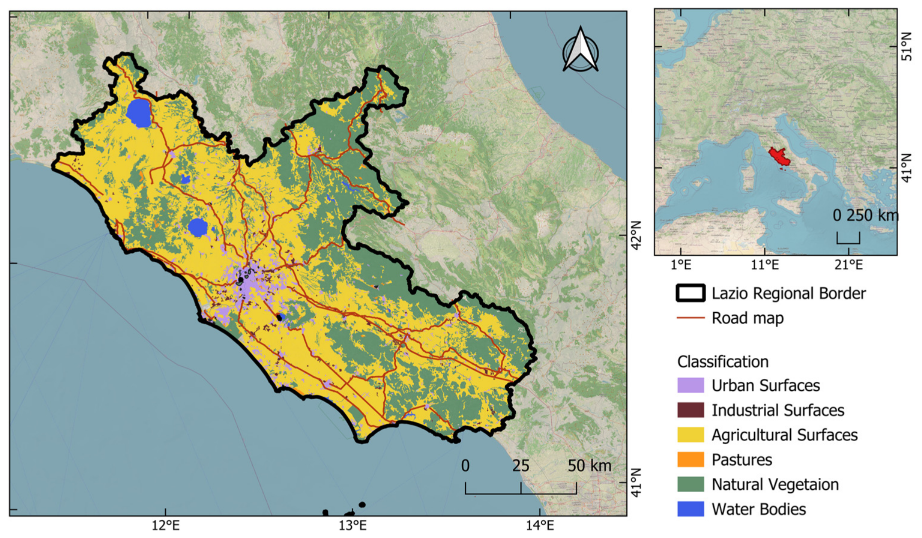
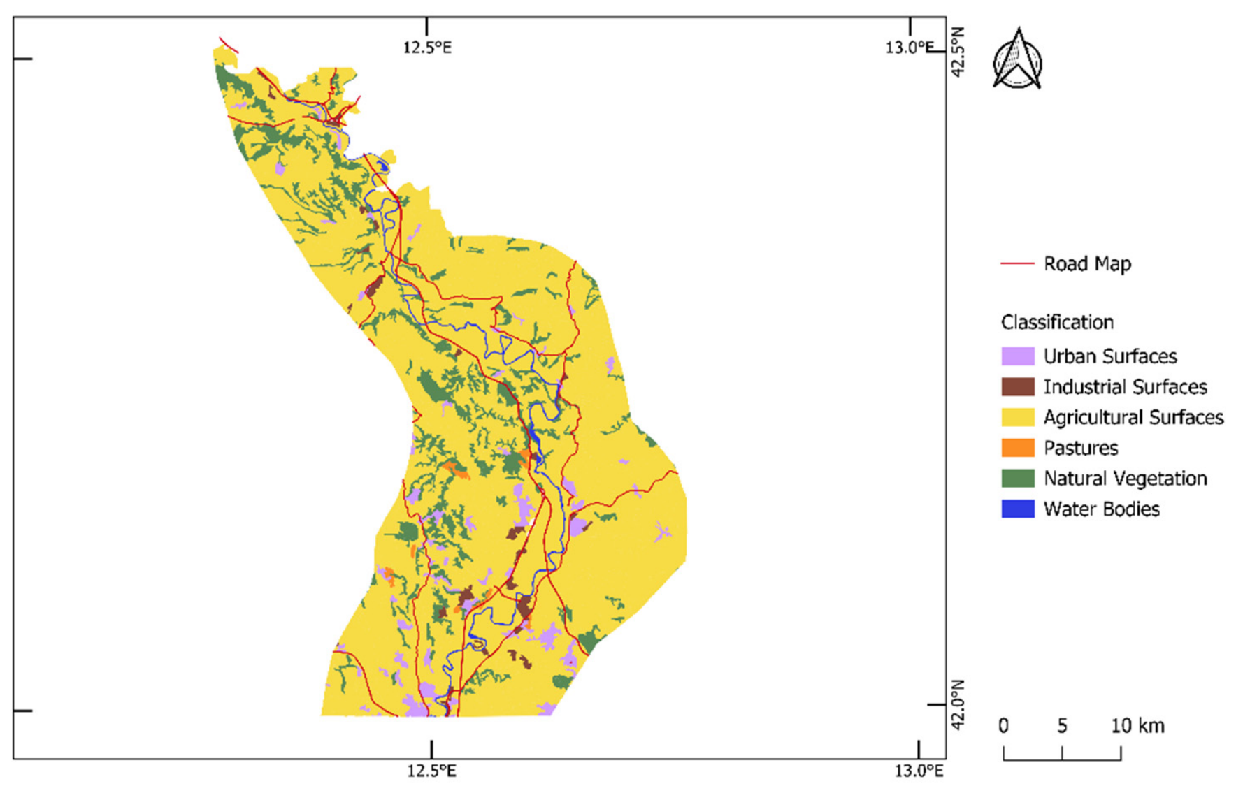
The Lazio region, located in central Italy, was selected as the study area because of its pronounced environmental and anthropogenic heterogeneity. Figure 1 provides the geographical context of the study area, showing the boundaries of the Lazio region and the land-cover classification, reinterpreted from the CORINE Land Cover (CLC) to derive environment categories consistent with the European Environment Agency (EEA) classification of air quality monitoring stations [25]. A road map (retrieved from OpenStreetMap, https://www.openstreetmap.org/relation/40784, accessed 8 July 2026) was also added to show the main road network. Only the principal highways and the main secondary roads are shown in the figure for the purposes of this study. A map showing the digital terrain model (DTM) [26] of the Lazio region is also included in the Supplementary Materials (Figure S1).

Urban surfaces are concentrated mainly in the Rome metropolitan area, clearly visible in purple in the center of the map, and in other major urban centers, while road corridors connect the coastal sector with inland areas and represent potential pathways of traffic-related emissions. Agricultural areas are widely distributed across lowland and peri-urban sectors, whereas natural vegetation dominates much of the inland, hilly, and mountainous territory. Industrial areas, coastal environments, and inland water bodies further contribute to the spatial heterogeneity of the region.

The coexistence of urban, industrial, agricultural, coastal, and rural environments results in strong contrasts in emission sources, land cover, and atmospheric conditions, making Lazio particularly suitable for investigating the spatial variability of satellite-derived trace-gas products. Previous studies have identified marked urban–rural gradients in trace-gas concentrations and aerosol loading, highlighting the influence of the Rome metropolitan area on surrounding environments [24,27]. Local meteorological processes, including sea-breeze circulation and boundary-layer dynamics, have been shown to play a key role in pollutant transport and accumulation within the region [28]. These characteristics provide a suitable framework for interpreting the spatial patterns of NO₂, HCHO, and CO and their relationships with regional emission sources and atmospheric processes.

2.2. Satellite Data

In this study, TROPOMI Products Algorithm Laboratory (PAL) Level 3 (L3-PAL) gridded products were used to investigate the spatial distribution of selected PM_2.5-related trace gases. L3-PAL products were retrieved from the S5P-PAL Data Portal (https://data-portal.s5p-pal.com/, last access: 2 July 2026) [29,30]. TROPOMI, a hyperspectral nadir-viewing spectrometer onboard the Sentinel-5 Precursor (S5P) mission, operates in a sun-synchronous ascending orbit with a local overpass time of approximately 13:30 [18,19]. The analysis focused on the tropospheric VCD of NO₂ [31], HCHO [32], and CO [33,34].

Monthly time-aggregated TROPOMI PAL products were employed to reduce the influence of short-term variability and to highlight persistent spatial patterns. They were selected as they are already provided as quality-screened and temporally aggregated gridded fields.

L3 PAL-products (including NO₂, HCHO and CO) downloaded from S5P-PAL Data Portal, are already filtered for Quality Assurance, by using: (i) qa_value > 0.75 for NO₂ data; and (ii) qa_value > 0.5 for HCHO and CO. NO₂ and HCHO PAL-products resulted to have, at the latitude of the study area, a grid-cell dimension of around 2.2 km × 1.8 km, while CO PAL a grid-cell dimension of 5 km × 3.6 km.

AOD data, which were included in the present study as a complementary indicator of aerosol burden, were retrieved from MODIS, a passive remote sensing instrument onboard NASA’s Terra and Aqua satellites [21]. The MODIS-MAIAC aerosol product (MCD19A2, Collection 6.1) was selected due to its high spatial resolution and improved aerosol retrieval performance (https://search.earthdata.nasa.gov/searcha; accessed on 25 August 2025). The MAIAC algorithm combines observations from both satellite platforms, providing AOD estimates at a spatial resolution of 1 km² and with observation frequency depending on satellite overpasses and atmospheric conditions [22]. For MODIS-MAIAC, AOD retrievals were restricted to the highest-quality pixels according to the AOD_QA product, whose reliability has been previously validated by Terenzi et al., 2025 [24]. Daily observations were averaged seasonally.

2.3. Data Processing and Seasonal Aggregation

Prior to the spatial and seasonal analyses, all satellite-derived products were harmonized under the same spatial, where possible, and temporal framework. The analysis covered the period from June 2018 to February 2024. Seasonal aggregates were estimated according to the conventional climatological definition of seasons: spring (MAM), summer (JJA), autumn (SON), and winter (DJF). For DJF, December was assigned to the following year.

All datasets were clipped to the Lazio administrative boundary and reprojected to the WGS84 coordinate reference system. Since NO₂ and HCHO had a higher spatial resolution compared to CO, CO was spatially harmonized onto the grid-cell dimension of NO₂, by resampling the coarser CO product to match the finer-resolution datasets using bilinear interpolation. The resampling procedure was performed in QGIS (version 3.34.15). This method assigns to each newly gridded pixel the distance-weighted average of the nearest four source-grid pixels, thus each interpolated value is constrained by the surrounding source values. For this reason, bilinear interpolation is suitable for spatially continuous data, as it preserves local gradients while avoiding returning artificial extremes and discontinuities [35,36]. Resampling was performed only to ensure spatial co-registration among variables and did not imply an increase in the native information content of the CO product.

2.4. Supporting Spatial Data

The identification and interpretation of the Regions of Interest (ROIs) also considered topographic information derived from the Continental Europe Digital Terrain Model (D.T.M) [26], with particular attention to valley areas (<450 m a.s.l.), where pollutant accumulation may be favored due to reduced ventilation and enhanced stability in low-elevation terrains [37]. The classification results were further interpreted in the context of findings reported in previous studies and subsequently compared with land-cover information [25] to investigate possible relationships between the observed air quality patterns and potential emission sources.

2.5. Ground-Based Monitoring Data

Hourly near-surface NO₂ concentrations were obtained from the ARPA Lazio air-quality monitoring network (https://www.arpalazio.it/, accessed on 10 July 2026) for the period June 2018–February 2024. Six stations located in the Sacco Valley–Lepini Mountains sector were selected (Alatri, Anagni S.F., Cassino, Colleferro O., Frosinone Mazzini, and Frosinone Scalo) based on their spatial location, continuity of the available records, and representation of different monitoring environments, including urban-background, urban-traffic, and industrial/suburban-background sites. Only observations validated by ARPA Lazio were retained, while missing or invalid records were excluded. Seasonal mean concentrations and boxplots were calculated from the valid hourly observations to assess the seasonal behavior and variability of NO₂ at each station.

2.6. Classification Approach

A classification approach based on K-means clustering was applied to multiple gaseous pollutants (NO₂, HCHO, and CO) to group areas with similar pollution characteristics. K-means is an unsupervised machine learning algorithm used for data clustering, which partitions unlabeled observations into homogeneous groups without requiring prior class definitions [38]. The classification was performed on seasonally averaged data to partially smooth the high spatial variability. The analysis was carried out using the SAGA “k-Means Clustering for Grids” tool in QGIS 3.44. The Hill-Climbing option was selected as the iterative optimization method, where the clustering is progressively improved by reallocating observations to reduce within-cluster variability. The algorithm was allowed to run for a maximum of 10 iterations, allowing the clustering solution to stabilize while keeping the computation time limited.

Before applying k-means clustering, the number of clusters was chosen based on a comparison of Elbow and Silhouette analysis performed on each gas; using both methods allows cluster selection to consider both internal compactness and separation among clusters [39]. In this study, the final number of clusters for each gas was chosen by comparing the results of Elbow and Silhouette analysis, selecting the solution that provided a balanced compromise between the two methods and physical significance depending on the gas distribution. Particularly, overlap between the distribution of values in clusters was considered, and a number of clusters that better allowed the identification of well-defined and diversified classes was generally favored. After applying the clustering procedure, eta-squared (η²) was calculated for the distribution of each gas in each cluster [40]. This allowed to assess the weight of each gas in the definition of classes and have a better understanding of phenomena seasonally influencing the clustering.

Clustering was first applied separately to each pollutant to evaluate individual spatial patterns and subsequently to the combined multi-pollutant normalized dataset to identify regions characterized by similar atmospheric composition. The spatial coherence of the clusters was then compared with elevation and land-cover information to support the definition of the ROIs. Land-cover and topographic information were therefore used as interpretative layers, rather than as input criteria for defining the clusters. While the AOD was not included in the multipollutant clustering, a spatial analysis was performed overlapping AOD data and the clustering results to explore the spatial consistency between the aerosol load and the precursors VCDs.

3. Results and Discussion

3.1. Seasonal Trends of Pollutants

Seasonal trends of the three selected trace-gas indicators were analyzed over the period 2018–2024 using tropospheric VCDs. The results for NO₂, HCHO and CO are presented in the following sections.

3.1.1. NO₂ Seasonal Trend

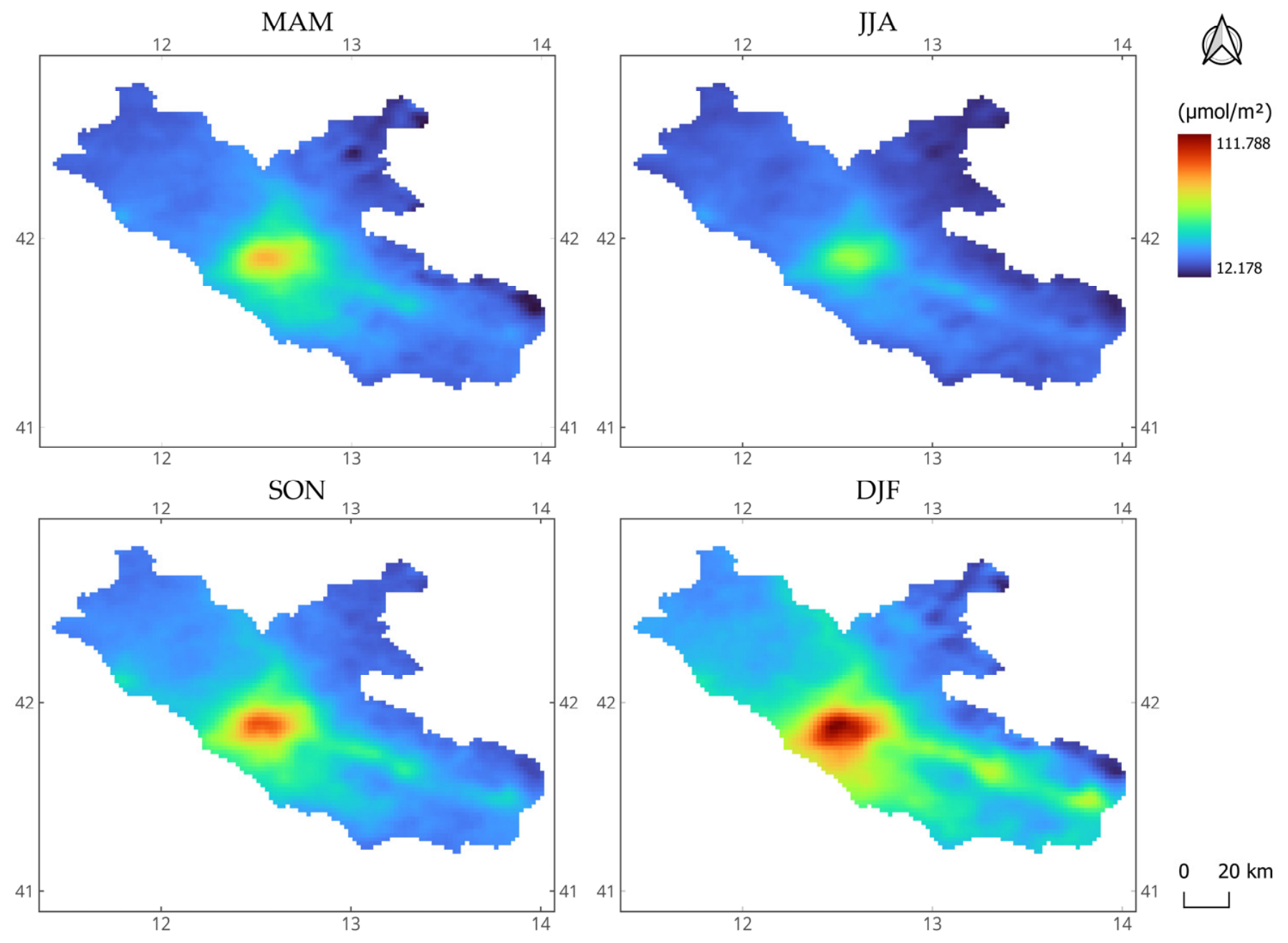
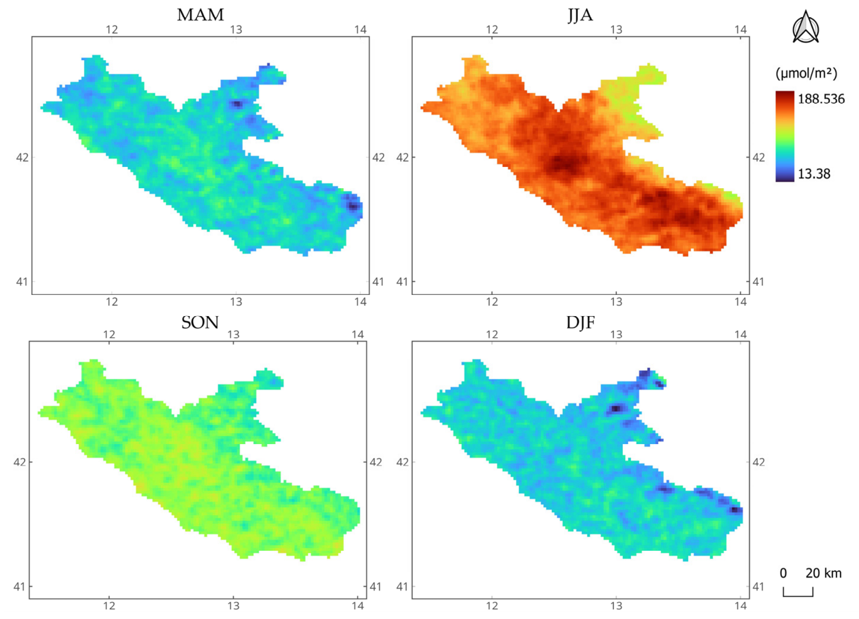
As shown in Figure 2, NO₂ tropospheric VCD values closely follow urban areas and main highways which can be spatially located using the study-area map reported in Figure 1, with a strong influence of anthropogenic emission sources, particularly in the metropolitan area of Rome, identified by the highest VCDs found in the center of the maps. Despite the presence of Rome, the NO₂ VCD spatial distribution in the rest of the region suggests that the observed NO₂ pattern is not only associated with the main urban agglomeration, but also with traffic-related linear emission sources and with the spatial organization of urban, industrial, and coastal sectors across the region. Tropospheric NO₂ follows the major road network particularly in valley areas (see Figure S1 of Supplementary Materials), where topographic confinement, reduced ventilation, and enhanced atmospheric stability may favor the accumulation of air pollutants [37]. In these areas, higher traffic intensity, the presence of local anthropogenic emission sources, and a high urbanization with limited natural vegetation further contribute to elevate NO₂ VCD values.

The highest values are observed around the Rome metropolitan area consistently in every season, confirming its role as the main regional hotspot. The seasonal statistics of NO₂ VCD over the Lazio region are reported in Table S1 of Supplementary Materials.

The analysis of the seasonal trend shows a clear seasonal variability. Levels peak during DJF, when the Rome hotspot becomes more intense; elevated values are also found toward the coastal area and along the main transport networks. This spatial pattern suggests a possible extension of the Rome pollution plume toward the coastal sector and surrounding regions. At the same time, the spatial distribution also highlights enhanced NO₂ levels outside the main metropolitan area, especially where major road corridors intersect densely populated, industrial, and peri-urban areas. This indicates that regional NO₂ variability is influenced by both concentrated urban emissions and more distributed anthropogenic sources. This increase is likely associated with higher emissions from domestic heating and road traffic, as the seasonal behavior of NO₂ is strongly linked to fossil-fuel combustion, which generally reaches its maximum during the cold season [41].

The lowest values are observed during JJA. Although the urban influence of Rome remains clearly visible, NO₂ levels are substantially reduced across the region. This decrease can be attributed to the shorter atmospheric lifetime of NO₂ under enhanced summertime photochemistry, promoted by stronger solar radiation and longer daylight hours, as well as the reduction of heating-related emissions during the warm season [42].

3.1.2. HCHO Seasonal Trend

Contrary to NO₂, formaldehyde exhibits a more widespread and homogeneous spatial distribution across the region (Figure 3), reflecting its predominantly secondary origin in the atmosphere [43]. HCHO is a ubiquitous VOC and an important intermediate product in the oxidation of both biogenic and anthropogenic non-methane VOCs (NMVOCs) and is commonly used as an indicator of VOC-related photochemical activity [44].

A marked seasonal cycle is evident, with the highest levels observed during JJA. In this season, elevated HCHO levels are distributed across most of the region, with particularly high values in the central and southern areas. When compared with the land-cover distribution reported in Figure 1, these areas correspond to a heterogeneous pattern of natural vegetation, agricultural surfaces, pastures, peri-urban areas, road corridors, and localized industrial or urban surfaces. Therefore, the observed HCHO enhancement cannot be attributed exclusively to vegetation. It also reflects the combined effect of regional photochemical activity and multiple VOC source types. This pattern is consistent with enhanced photochemical activity driven by higher temperatures, stronger solar radiation, and increased emissions of biogenic VOCs, which promote the formation of secondary formaldehyde. In particular, isoprene (C₅H₈), one of the main precursors of HCHO at the local scale, is emitted at high rates by vegetation during the warm season and is rapidly oxidized in the presence of NO_x [45,46], likely caused by heat stress, leading to enhanced HCHO production [47]. Moreover, the high temperatures and frequent drought conditions that characterize JJA can further stimulate biogenic VOC (BVOC) emissions as part of plant physiological responses to thermal and water stress, thereby contributing to the seasonal enhancement of atmospheric HCHO [48]. At the same time, anthropogenic VOC emissions from traffic, industrial activities, solvent use, and other urban or peri-urban sources may also contribute to HCHO formation, especially where these sources overlap with high photochemical reactivity and NO_x availability.

In contrast, DJF is characterized by the lowest mean HCHO levels at the regional scale. Reduced solar radiation, lower temperatures, and weaker biogenic emissions limit the oxidation processes responsible for HCHO production, resulting in a substantial seasonal decrease. The winter reduction also suggests that, although anthropogenic VOC sources may persist throughout the year, photochemical conditions are less favorable for secondary HCHO formation.

Unlike NO₂, no distinct urban hotspot is observed over the Rome metropolitan area, suggesting that regional photochemical production, and biogenic sources play a more important role than local combustion emissions in controlling the spatial distribution of HCHO across the Lazio region.

3.1.3. CO Seasonal Trend

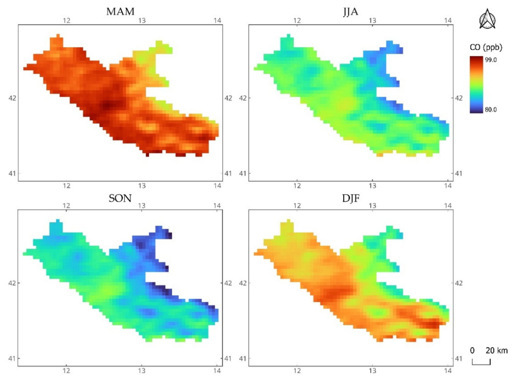
The seasonal trend of CO exhibits a relatively homogeneous spatial distribution across the Lazio region, with concentrations generally decreasing from the western and southwestern sectors toward the eastern mountainous areas, as shown in Figure 4.

Higher values are mainly associated with the lowland areas, where urban settlements, agricultural surfaces, and the main road network are concentrated, whereas lower concentrations characterize the mountain region, which is dominated by natural vegetation and lower anthropogenic presence.

A clear seasonal variability is also observed. CO VCDs are highest during MAM and remain relatively elevated in DJF, while JJA and SON exhibit the lowest values. The enhanced levels during spring and winter are consistent with the greater contribution of combustion-related emissions and with atmospheric conditions that favor CO accumulation [49]. Conversely, the lower concentrations observed during summer can be explained by more efficient atmospheric mixing and by the enhanced oxidation of CO by hydroxyl (OH) radicals under stronger solar radiation [50].

Unlike NO₂, CO does not display a distinct hotspot over the Rome metropolitan area, suggesting that its spatial distribution is less affected by localized emission sources and more strongly influenced by diffuse combustion activities, mainly of anthropogenic origin, occurring across the region. Moreover, the longer atmospheric lifetime of CO favors regional transport [49], making the identification of local emission sources more challenging. Therefore, although both NO₂ and CO are associated with combustion processes, NO₂ is more closely associated with localized emission sources, whereas CO, due to its longer atmospheric lifetime, better captures diffuse combustion signals and regional transport processes.

3.2. K-Means Classification for Individual Trace Gas

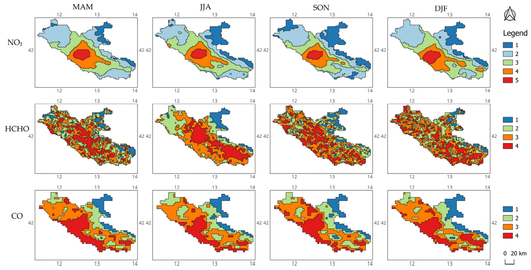
The results from the Silhouette and Elbow analysis (Figures S2–S4 of Supplementary Materials), together with results of the spatial distributions, allowed us to choose the more suitable number of clusters for each gas. The chosen values of clusters are k = 5 for NO₂, k = 4 for HCHO, and k = 4 for CO. While the Elbow results generally favored a reduced number of clusters, the Silhouette score always remained above 0.5, indicating reasonable values of k [39]. Therefore, the number of clusters was selected based on a statistical performance and the physical interpretability of the resulting spatial patterns. Particular consideration was given to spatial coherent regions rather than small, isolated or fragmented patches, while avoiding overlapping between values in different classes. A k-means classification was then performed for each pollutant separately.

Figure 5 shows the classification patterns for each selected gas.

Both CO and NO₂ exhibit a clear and a spatially well-defined classification, with only minor seasonal variations observed across the different periods analyzed for CO. NO₂ remains overall stable throughout all seasons, reflecting the persistence of combustion-related source areas, particularly around the Rome metropolitan area and along the main transport pathways. HCHO, on the other hand, displays a more pronounced and distinct classification during the JJA, when its absolute concentrations are higher compared to other seasons.

3.3. Combined Classification and Definition of ROIs

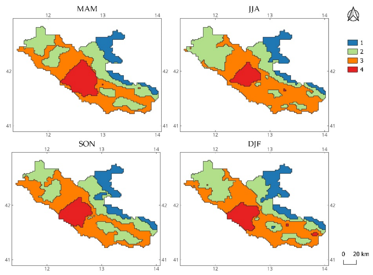
Following the preliminary analysis of each trace gas separately, CO, HCHO, and NO₂ were combined to define the regions of interest (ROIs) through a multivariate clustering approach. The individual-gas clustering and the multivariate clustering had different objectives. The former was used as a diagnostic step to describe the spatial variability of each trace gas separately, whereas the latter was designed to identify spatially coherent atmospheric regimes emerging from the joint behavior of NO₂, HCHO, and CO. Therefore, the same k was not imposed across the individual pollutants. To perform the multi-pollutant classification, a common k = 4 was chosen as a compromise solution supported by the Elbow and Silhouette analyses and further evaluated according to the spatial coherence and physical interpretability of the clusters. Although NO₂ alone showed higher spatial variability and was described with k = 5, using k = 5 increased the influence of the higher spatial variability of NO₂ on the combined classification, producing a more fragmented spatial pattern for CO and HCHO, with classes characterized by similar ranges of values. Therefore, k = 4 was retained to obtain a balanced multi-gas classification that preserved the combined information of NO₂, HCHO, and CO while maintaining a clear spatial interpretation. The resulting classification was designed to identify areas characterized by similar atmospheric patterns based on the joint variability of the three pollutants. The spatial distribution of the resulting clusters is shown in Figure 6.

Depending on the season, the spatial distribution of the four clusters changes (Figure 6), although their ranking consistently reflects progressively increasing multi-gas levels from the Blue to the Red class. The relative contribution of individual species to this gradient varies seasonally, reflecting changes in emission sources, photochemical activity, and atmospheric dispersion processes.

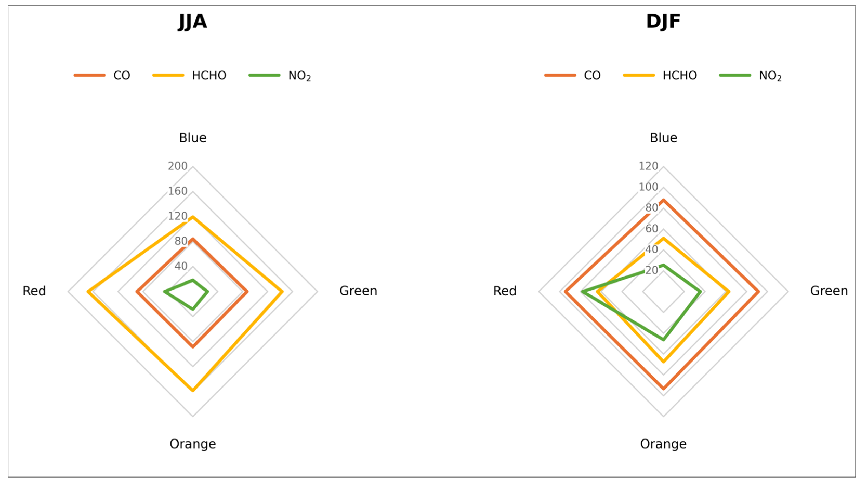
Figure 7 highlights differences in the mean seasonal VCDs of CO, HCHO and NO₂ for each cluster. The complete set of seasonal cluster values were used to quantify the percentage variation between the Blue and Red classes and are reported in Table S2 of the Supplementary Materials. JJA and DJF were selected because they represent contrasting seasonal conditions, characterized respectively by enhanced photochemical activity and by stronger accumulation of combustion-related pollutants under less dispersive atmospheric conditions.

In JJA (Figure 7, left), all three variables increase progressively from the Blue cluster to the Red cluster. Based on the raw seasonal cluster values reported in Table S2 of the Supplementary Materials, the strongest relative increase is observed for NO₂, which rises from 18.2 to 45.1 µmol m⁻² (+147.8%), followed by HCHO, which increases from 119.4 to 168.1 µmol m⁻² (+40.8%). CO shows only a limited increase, from 84.2 to 89.5 ppb (+6.3%), remaining comparatively homogeneous across the four classes. These results indicate that the summer cluster separation reflects the combined variability of the three gases. This pattern is consistent with the combined influence of anthropogenic NO_x-related emissions, VOC-related photochemical activity, and the broader-scale contribution of CO. In DJF (Figure 7, right), CO and NO₂ increase progressively from the Blue cluster to the Red cluster, whereas HCHO reaches its maximum in the Orange cluster and slightly decreases in the Red cluster. CO increases from 87.9 to 94.4 ppb (+7.4%), HCHO from 51.1 to 67.4 µmol m⁻² (+31.9%) from the Blue to the Orange cluster, before decreasing to 63.6 µmol m⁻² in the Red cluster; NO₂ rises from 25.3 to 77.8 µmol m⁻² (+207.5%). The winter gradient is therefore particularly driven by NO₂, which shows the largest relative increase among the three species, consistent with the stronger influence of combustion-related emissions and less favorable dispersion conditions during the cold season. CO also contributes to the winter multi-pollutant structure as a combustion-related tracer, although its variation among clusters remains comparatively limited.

Eta-squared (η²) was calculated to assess the weight of each gas on the k-means classification.

Table 1. Eta-squared (η²) values for each gas and season.

	CO	HCHO	NO2
MAM	0.82	0.24	0.73
JJA	0.74	0.70	0.76
SON	0.84	0.49	0.63
DJF	0.84	0.33	0.8

reports η² for each gas and season.

Higher values suggest a greater portion of variance explained by the specific variable. Thus, CO is the gas that most contributes to the k-means classification, as it shows high values in each season. HCHO has the highest seasonal variability, with the highest value in JJA, while NO₂ shows high values in each season, especially in winter and summer, where it surpasses CO. Thus, the summer η² values for all gases reflect the high level of atmospheric complexity, and as such anthropogenic emissions are complemented by biogenic and photochemical summer sources. On the other hand, in winter CO and NO₂ have similar impacts on the definition of clusters, while HCHO has less influence. This is due to high anthropogenic emissions, such as transport and heating, and atmospheric stagnation phenomena.

MAM and SON show intermediate values. MAM marks the transition to the warmer months, when the photochemical and biogenic sources of HCHO are still not fully active and the influence of this gas on clustering is at its lowest (η² equal to 0.24). In SON the influence of CO to the clustering is at its highest, while HCHO shows an intermediate value between summer and winter.

Comparing this insight with the low relative amplitude of the mean values (between 5.7% and 7.4%) and standard deviation values (around 1% of the mean) for CO, this gas contributes substantially to the separation of the clusters despite its relatively limited within-cluster variability, and may therefore represent a relatively homogeneous combustion-related background across the classified areas. NO₂ has generally slightly lower η² values, but shows a sharp increase in mean value between the orange and red clusters in all seasons (an increase of 60% to 70% between Orange and Red clusters compared to a 140–200% total increase between Red and Blue clusters), suggesting NO₂ probably drives the definition of the Red clusters, where transportation-related pollution is particularly present. Similarly, HCHO shows the sharpest increase between the Blue and Green clusters, thus driving this portion of the classification.

These results show that the Blue-to-Red cluster ranking represents a generally increasing multi-gas gradient in both seasons, but the relative weight of individual species changes seasonally. In JJA, cluster separation is more strongly influenced by HCHO and NO₂, whereas in DJF it is dominated by the marked increase in NO₂, with CO providing a more homogeneous combustion-related background contribution. Such variability likely reflects seasonal changes in emission sources, photochemical activity, and atmospheric dispersion processes.

3.3.1. Definition of ROIs

The seasonal multi-pollutant classification helped to highlight three main ROIs, graphically represented in Supplementary Materials Figure S5: the Tiber Valley, the Sacco Valley, and the Lepini Mountains. To quantitatively support the interpretation of the selected ROIs, seasonal mean values of NO₂, HCHO, and CO, together with the values of the whole Lazio region, were extracted for each region and are shown in

Table 2. Seasonal tropospheric VCD mean values of NO₂, HCHO, and CO in the selected ROIs and for the whole Lazio region.

(a) NO2 Mean (µmol m−2).
ROI	MAM	JJA	SON	DJF
Lazio region	31.34	26.63	35.9	42.52
Tiber Valley	36.97	30.89	41.02	46.49
Sacco Valley	32.44	28.38	37.72	49.42
Lepini Mountains	33.55	27.36	35.92	42.67
(b) HCHO mean (µmol m−2)
ROI	MAM	JJA	SON	DJF
Lazio region	65.12	149.3	93.08	63.09
Tiber Valley	70.07	163.73	98.21	63.34
Sacco Valley	64.01	168.64	95.81	69.58
Lepini Mountains	71.35	156.14	63.98	92.63
(c) CO mean (ppb)
ROI	MAM	JJA	SON	DJF
Lazio region	95.24	87.56	85.7	91.89
Tiber Valley	96.39	88.64	87.14	93.29
Sacco Valley	96.09	88.31	86.31	93.71
Lepini Mountains	94.49	86.83	84.43	90.51

. The whole set of the statistical values is reported in Supplementary Materials (Table S3).

These regions were selected because they represent spatially coherent features in the seasonal classifications and include different environmental conditions ranging from peri-urban valley regions, industrially developed lowlands, and cleaner mountains. These results indicate that the identified ROIs represent not only different pollution intensities, but also distinct atmospheric regimes characterized by varying contributions of combustion-related and photochemically driven atmospheric tracers. Thus, the ROIs should be interpreted as satellite-derived atmospheric regimes, not simply as predefined geographical units. Consequently, the multivariate approach provides a more comprehensive characterization of atmospheric variability than analyses based on individual trace gases alone.

A pronounced and spatially coherent pattern was also identified over the metropolitan area of Rome. However, Rome was not addressed in the present study as a specific ROI, as the urban area represents the dominant and already well-characterized regional hotspot [51]. The Rome metropolitan area is instead used as a reference source region for interpreting spatial gradients toward surrounding peri-urban and non-metropolitan areas, where the interaction between transported pollution, local emissions, and topography is less well characterized.

3.3.2. Focus on the Tiber Valley

The Tiber Valley (Figure 8) is characterized by the possible influence of pollution plumes originating from the Rome metropolitan area, combined with local emission sources and the effects of complex terrain. Valley morphology may favor pollutant accumulation through topographic confinement, reduced ventilation, and enhanced atmospheric stability [37].

The area was selected because, despite its marked environmental heterogeneity, it has received comparatively limited attention in previous studies. The valley is predominantly rural, with agricultural land representing the dominant land-cover type and supporting intensive agricultural activities along the irrigated Tiber River corridor. At the same time, the valley is crossed by major transportation infrastructures and is affected by nearby industrial activities, particularly in the southern sectors. These anthropogenic sources, together with the topographic confinement and reduced ventilation associated with the valley morphology, contribute to heterogeneous pollution conditions and spatially variable VCDs of atmospheric precursors. This interpretation is consistent with the seasonal mean values reported in [27], where the Lazio regional mean is also reported as a regional-scale reference. Within this context, the Tiber Valley shows NO₂ mean values higher than the regional average in all seasons, with DJF values reaching 46.49 µmol m⁻² compared with 42.52 µmol m⁻² for the whole Lazio region. This indicates that, despite its predominantly rural and agricultural character, the selected ROI is affected by atmospheric conditions above the regional mean for combustion-related trace-gas indicators. HCHO also shows a marked summer enhancement, reaching 163.73 µmol m⁻² in JJA compared with 149.30 µmol m⁻² for the Lazio region, suggesting enhanced VOC-related photochemical activity during the warm season. CO values are also slightly higher than the regional average, especially in MAM and DJF, supporting the possible contribution of combustion-related sources and transported pollution. Consistent with previous studies in the area [27], the observed patterns suggest the coexistence of local emissions and transported pollutants, resulting in a complex air-quality regime. The combination of diverse emission sources and terrain-induced transport processes makes the Tiber Valley a particularly suitable case study for investigating spatial variability in atmospheric composition within peri-urban environments.

3.3.3. Focus: On the Sacco Valley and the Lepini Mountains

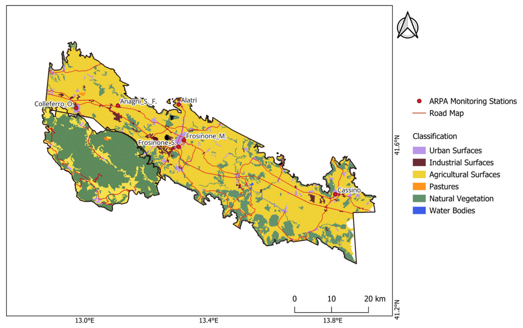
The Sacco Valley and the Lepini Mountains are reported together in Figure 9, as a unique sector, due to their close geographical proximity and their strongly contrasting environmental and pollution characteristics. This ROI encompasses two neighboring areas that differ substantially in terms of topography, land cover, and anthropogenic pressure.

The Sacco Valley showed elevated pollution levels due to the combined influence of urban emissions, industrial activities, and road traffic. This area has long been recognized as one of the main pollution hotspots in central Italy, owing to the concentration of industrial settlements and major transportation corridors, and has been extensively investigated because of its environmental and public health implications [52]. For this reason, it is widely monitored through a network of air quality and meteorological stations operated by ARPA Lazio (https://www.arpalazio.it/ambiente/aria/sistema-di-monitoraggio, accessed 10 July 2026). As shown in Figure 9, the ARPA stations are mainly located along the inhabited and industrialized valley floor, close to urban centers, peri-urban areas, and major transport corridors.

In addition, the Sacco Valley’s basin-like morphology shares some similarities, albeit on a smaller scale, with that of the Po Valley, favoring pollutant build-up under stable atmospheric conditions.

In contrast, the nearby Lepini Mountains exhibited lower NO₂ and CO levels despite their geographical proximity to the valley, consistent with their higher elevation, lower anthropogenic pressure, and extensive natural vegetation. This contrast is also evident in the seasonal mean values [53], with the Lepini Mountains showing lower DJF for NO₂ and CO than the Sacco Valley, respectively 42.67 µmol m⁻² and 90.51 ppb. However, HCHO shows a distinct behavior, with relatively high values in both JJA and DJF and a DJF mean value of 92.63 µmol m⁻², higher than those observed in the valley ROIs. This suggests a different atmospheric regime, likely influenced by biogenic VOC emissions, secondary photochemical processes, and possible interactions with transported pollutants from adjacent areas. The higher elevation, lower anthropogenic pressure, and the presence of extensive natural and forested areas likely enhance atmospheric dilution and deposition processes, mitigating pollutant accumulation [53]. Nevertheless, marginal sectors of the Lepini Mountains still showed evidence of influence from adjacent polluted areas, suggesting that pollutant transport from the Sacco Valley can affect surrounding mountainous environments under favorable meteorological conditions. The juxtaposition of these two contrasting environments provides a valuable framework for assessing how differences in emissions and topography shape local air quality over relatively short spatial scales.

3.4. Ground-Based Observations in the Sacco Valley

A focused analysis was also performed over the Sacco Valley–Lepini Mountains sector to compare the spatial information provided by satellite observations with the distribution and seasonal behavior of ground-based monitoring sites. This sector was selected because active ARPA monitoring stations are available, whereas no active ARPA stations are currently present in the Tiber Valley. NO₂ was selected as the representative pollutant for this comparison because it was the only species consistently monitored across the ARPA network, while observations of other pollutants considered in this study were available only at a limited number of stations or were not available.

As discussed in Section 3.2, the ARPA monitoring stations are mainly located at strategic sites along the inhabited and industrialized valley floor, close to urban and peri-urban areas as well as the major transport corridors. Consequently, although these stations provide valuable information on local near-surface NO₂ variability, their spatial distribution does not continuously cover the surrounding agricultural, natural, and mountainous areas, nor the inter-station gradients along the valley.

To facilitate the interpretation of the spatial distribution, the monitoring stations, presented in Figure 9, are identified hereafter by codes rather than by their full names. The correspondence between the station codes and the respective monitoring stations is reported in

Table 3. Seasonal NO₂ tropospheric VCD values in the Sacco Valley corresponding to the ARPA monitoring stations.

Station Code	ARPA Monitoring Station	Station Type	Latitude	Longitude	NO2 DJF (µmol m−2)	NO2 MAM (µmol m−2)	NO2 SON (µmol m−2)	NO2 JJA (µmol m−2)
ALA	Alatri	Urban Background	41.72729	13.33828	50.30	31.43	35.75	25.60
ASF	Anagni S. F.	Urban Background	41.73195	13.14033	56.90	40.56	47.51	35.58
CAS	Cassino	Urban Traffic	41.48845	13.83072	64.53	31.70	42.61	28.51
COL	Colleferro O.	Industrial, Suburban Background	41.73045	13.00406	57.09	41.18	44.71	31.95
FRM	Frosinone M.	Urban Background	41.63960	13.34897	61.96	38.52	43.65	31.01
FRS	Frosinone S.	Urban Traffic	41.62431	13.33091	64.61	39.24	45.32	32.47

, which also summarizes the mean seasonal tropospheric NO₂ VCD values extracted at the geographical coordinates of each monitoring station.

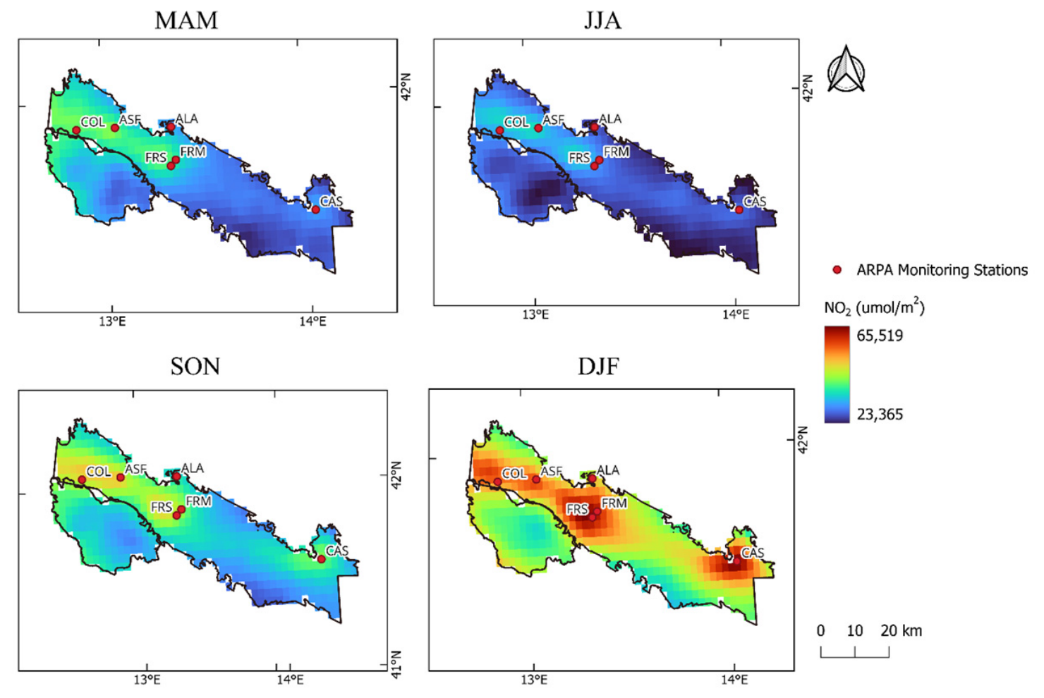
The seasonal NO₂ tropospheric VCD maps reported in Figure 10 show a coherent seasonal behavior, with reduced values during JJA and enhanced levels during DJF.

The VCD values extracted at the ARPA station locations confirm this seasonal pattern, with DJF maxima and JJA minima at all sites. However, these values should not be interpreted as direct equivalents of ground-level concentrations, because they represent column-integrated NO₂ amounts. Their main contribution is therefore to provide the spatial context of NO₂ column enhancements over the valley, rather than a point-by-point replication of near-surface measurements. In winter, the satellite signal highlights broader NO₂ enhancements along the valley and transport-related corridor, including areas between monitoring stations and sectors not directly sampled by the ground network. This spatial continuity cannot be fully resolved from point-based observations alone.

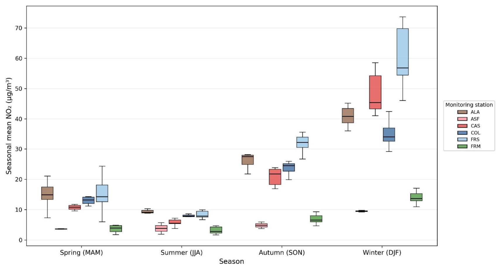
The ARPA seasonal boxplots shown in Figure 11 confirm a clear seasonal cycle in near-surface NO₂, with lower values during JJA and higher values during DJF, particularly at stations located in more urbanized or traffic-influenced contexts (e.g., ALA, CAS and FRS stations).

A further limitation concerns the spatial representativeness of ground-based observations in relation to the natural areas of the Lepini Mountains. The forested surfaces characterizing this sector may influence atmospheric NO₂ levels through vegetation uptake and deposition processes [54], while forest–urban edge effects may locally modify pollutant gradients [55]. However, the current ARPA monitoring network is mainly located in anthropized areas along the valley floor, and no station directly represents the surrounding forested and mountainous environments. Therefore, satellite observations provide useful complementary information by describing the spatial continuity of NO₂ columns across both monitored and unmonitored sectors. Some apparent differences between ground-based measurements and satellite-derived VCDs can also be interpreted in relation to station location and valley morphology. ALA station, for example, may be affected by relevant local near-surface NO₂ contributions, as suggested by the ground-based observations, but its position close to the margin of the valley may limit the development of persistent stagnation and columnar accumulation detectable in the satellite VCD field. By contrast, ASF and COL stations are more closely connected to the main valley corridor, where industrial activities, road traffic, and local accumulation processes may contribute to broader NO₂ column enhancements. This suggests that the VCD field is not only sensitive to local emissions at individual sites, but also to the spatial integration of emissions and accumulation processes over the valley.

A similar interpretation applies to the Frosinone area. FRM shows lower near-surface NO₂ levels than FRS, consistent with its urban background classification and lower direct exposure to traffic-related emissions. Nevertheless, the satellite VCD field indicates enhanced NO₂ over the broader Frosinone urban and valley context. This suggests that the ground-based measurement correctly represents the local monitoring environment, while satellite observation provides the wider spatial framework in which that site is embedded.

Ground stations remain essential for characterizing local exposure conditions and specific monitoring environments, such as urban background or traffic-influenced sites. Conversely, TROPOMI provides a spatially continuous view of NO₂ over the whole sector, allowing point-based measurements to be interpreted within a broader valley-scale context. The added value of the satellite-based approach therefore lies in identifying spatial gradients, areas characterized by enhanced columnar NO₂ levels, inter-station variability, and potentially unmonitored sectors influenced by anthropogenic NO₂ sources.

3.5. AOD Seasonal Trend and Spatial Overlay Analysis

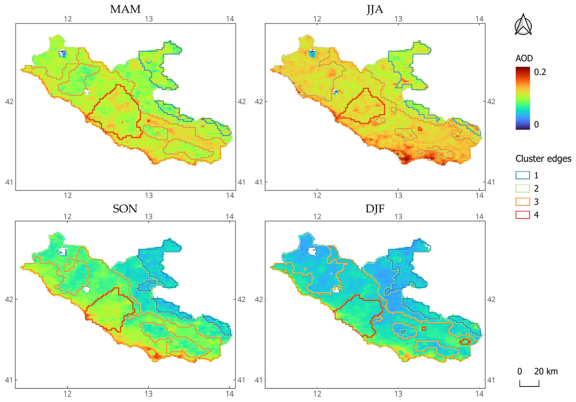
To complement the analysis of trace gases the seasonal variability of AOD was also investigated over the same period. The clusters identified through the multivariate classification of gases were consequently overlaid onto the AOD seasonal maps. Although AOD does not constitute a direct measure of near-surface PM_2.5 concentration, it provides a column-integrated indicator of aerosol loading and can therefore be used as complementary information to interpret the spatial patterns identified from trace-gas observation. Figure 12 shows the seasonal distribution of AOD across the Lazio region and the overlaid clusters.

A marked seasonal cycle is evident, with maximum values occurring during JJA and minimum values during DJF, reflecting the combined influence of enhanced photochemical activity and possible episodic long-range transport events of dust typical of the Mediterranean basin in summer [56,57]. A persistent coastal enhancement is also visible throughout the year, likely associated with marine aerosols and boundary-layer dynamics. However, this pattern may also partly reflect retrieval uncertainties near the coastline, where values within ±1–3 pixels from the coastline may be affected by cloud-mask artifacts (typically over detection), positive AOD biases, and surface bidirectional reflectance (BRF) uncertainties [22]. Seasonal mean AOD values for the selected ROIs and for the Lazio regional average are reported in

Table 4. Seasonal mean AOD values for the selected ROIs and Lazio regional average.

Area	SON AOD Mean	DJF AOD Mean	MAM AOD Mean	JJA AOD Mean
Lazio Regional Mean	0.084	0.063	0.107	0.123
Tiber Valley	0.084	0.061	0.109	0.118
Sacco Valley	0.088	0.069	0.119	0.124
Lepini mountains	0.077	0.056	0.106	0.124

, allowing a quantitative comparison between the aerosol burden observed in the ROIs. The whole set of the statistical values is reported in Supplementary Materials (Table S4).

In seasons characterized by lower regional aerosol loading and a weaker influence of large-scale external contributions (SON and DJF), the AOD distribution retains clearer spatial contrasts, allowing the contribution of local and regional processes to be more readily distinguished. The Sacco Valley consistently exhibits the highest AOD values, and the contrast with the regional background (Lazio region) is particularly evident during DJF and MAM. This behavior is also clearly visible in the difference between the Sacco Valley and the Lepini Mountains in all seasons except JJA. During summer, the influence of Saharan dust transport likely increases aerosol loading over the entire region [58,59], reducing spatial contrasts and producing a more homogeneous regional AOD distribution.

The AOD spatial distribution generally reflects the distribution of multi-gas clusters in all seasons except JJA. Particularly, in MAM, SON and DJF, the AOD precisely overlaps with the classes 1 and 2, where its values are lower. The mountain regions (class 1) are always well visible in the AOD distribution, as well as the vegetated regions of the Lepini Mountains and in the north of Lazio, identified by class 2. Classes 3 and 4, coincide with regions where AOD values are higher. In class 3, the AOD distribution reflects the edges of the class in correspondence of the ROIs of the Lepini Mountains and Sacco Valley, where increased concentrations of aerosol precursor gases, particularly NO₂ and HCHO, are found. This pattern suggests a possible contribution of local precursor emissions to secondary aerosol formation. Accordingly, in coastal regions, where there is likely a stronger contribution of non-gaseous aerosol, the AOD expresses a local distribution despite the class. Class 4 does not coincide with a clear peak in AOD, likely because this class is strongly influenced by NO₂ distribution over Rome, while the AOD reflects the combined contribution of different aerosol types within the atmospheric column. Moreover, in JJA the AOD and cluster distribution diverges; this result suggests that high inputs of aerosol and dust occurring during the summer overcome local emission sources and gas-derived aerosol, making the AOD spatial trend apparently independent from the gas distribution.

4. Conclusions and Further Steps

The combined use of satellite observations and clustering analysis performed in the present paper allowed the identification of major pollution hotspots, cleaner background areas, and transition zones with mixed atmospheric conditions. Satellite-based observations provide a powerful complement to ground-based monitoring for investigating, monitoring, and mitigating PM_2.5-related trace-gas indicators and aerosol loading. K-means clustering successfully identified major hotspots such as the Sacco Valley, cleaner environments such as the Lepini Mountains, and mixed-condition regions such as the Tiber Valley. These areas should not be interpreted simply as predefined geographical units, but as satellite-derived atmospheric regimes emerging from the combined seasonal behavior of NO₂, HCHO, and CO VCDs. The comparison with land cover data highlighted the dominant role of anthropogenic emissions in highly polluted areas, such as the Sacco Valley, while also suggesting a possible influence of elevation, lower anthropogenic pressure, and extensive natural vegetation on the observed spatial gradients.

Seasonal patterns of NO₂, HCHO, and CO were analyzed and subsequently combined through K-means clustering to identify areas characterized by similar multi-gas spatial patterns. These areas therefore reflect similarities in the satellite-observed behavior of the selected trace gases, linked to emissions and atmospheric chemistry, rather than generic atmospheric conditions. This data-driven approach allows atmospheric variability to be assessed independently of administrative boundaries or single land-cover classes, providing a spatially continuous framework for interpreting regional air-quality patterns.

TROPOMI provides a spatially continuous view of tropospheric NO₂ columns, whereas ground stations describe local conditions at selected points. Therefore, the added value of the satellite-based approach lies in extending the interpretation from discrete monitoring sites to a continuous regional framework, supporting the identification of spatial gradients, areas characterized by enhanced NO₂ levels, and potentially unmonitored areas influenced by anthropogenic NO₂ sources. This capability is particularly relevant for the Tiber Valley, where the absence of active ARPA stations limits the availability of spatially distributed ground-based information. More generally, the proposed framework is particularly useful in heterogeneous regions where conventional monitoring networks are sparse or unevenly distributed. The seasonal agreement between satellite and ground-based observations provides qualitative support for the interpretation of the satellite-derived spatial patterns, while reflecting the different atmospheric quantities and spatial scales represented by the two datasets.

This integrated analysis supports the development of seasonal and localized emission reduction strategies and improves the understanding of atmospheric processes affecting air quality in the Lazio region. Because it relies on openly available satellite products and ancillary land-cover information, the approach is potentially transferable to other regions characterized by complex terrain, mixed emission sources, or limited ground-based monitoring. It may also support decision-makers in identifying priority areas for monitoring optimization and targeted mitigation actions. Future work may include the integration of ground-based observations to further refine source attribution and improve air quality forecasting.

References

1. Liu, C.; Chen, R.; Sera, F.; Vicedo-Cabrera, A.M.; Guo, Y.; Tong, S.; Lavigne, E.; Matus Correa, P.; Valdes Ortega, N.; Achilleos, S.; et al. Interactive effects of ambient fine particulate matter and ozone on daily mortality in 372 cities: Two stage time series analysis. BMJ 2023, 383, e075203. [Google Scholar] [CrossRef] [Scilit]
2. International Agency for Research on Cancer. IARC Monographs Group 1 Classification List. 27 March 2026. Available online: https://monographs.iarc.who.int/list-of-classifications (accessed on 27 March 2026).
3. The European Parliament. Directive (EU) 2024/2881 of the European Parliament and of the Council of 23 October 2024 on Ambient Air Quality and Cleaner Air for Europe (Recast). 2024. Available online: http://data.europa.eu/eli/dir/2024/2881/oj (accessed on 27 March 2026).
4. Kang, S.; Choi, S.; Ban, J.; Kim, K.; Singh, R.; Park, G.; Kim, M.-B.; Yu, D.-G.; Kim, J.-A.; Kim, S.-W.; et al. Chemical characteristics and sources of PM2.5 in the urban environment of Seoul, Korea. Atmos. Pollut. Res. 2022, 13, 101568. [Google Scholar] [CrossRef] [Scilit]
5. Thangavel, P.; Park, D.; Lee, E.Y.-C. Recent Insights into Particulate Matter (PM2.5)-Mediated Toxicity in Humans: An Overview. Int. J. Environ. Res. Public Health 2022, 19, 7511. [Google Scholar] [CrossRef] [Scilit] [PubMed]
6. Yin, P.-Y. A Review on PM2.5 Sources, Mass Prediction, and Association Analysis: Research Opportunities and Challenges. Sustainability 2025, 17, 1101. [Google Scholar] [CrossRef] [Scilit]
7. Alam, M.J.; Karim, I.; Zaman, E.S.U. Seasonal dynamics and trends in air pollutants: A comprehensive analysis of PM2.5, NO2, CO, SO2 and O3 in Houston, USA. Air Qual. Atmos. Health 2025, 18, 2625–2642. [Google Scholar] [CrossRef] [Scilit]
8. Jeon, H.; Ko, D.-H.; Kim, W.; Bae, E.M.-S. Influence of agricultural ammonia and waste burning on PM2.5 composition in a livestock-intensive suburban region. Environ. Geochem Health 2026, 48, 278. [Google Scholar] [CrossRef] [Scilit] [PubMed]
9. Wang, M.; Kim, R.Y.; Kohonen-Corish, M.R.J.; Chen, H.; Donovan, C.; Oliver, E.B.G. Particulate matter air pollution as a cause of lung cancer: Epidemiological and experimental evidence. Br. J. Cancer 2025, 132, 986–996. [Google Scholar] [CrossRef] [Scilit] [PubMed]
10. Casallas, A.; Castillo-Camacho, M.P.; Guevara-Luna, M.A.; González, Y.; Sanchez, E.; Belalcazar, E.L.C. Spatio-temporal analysis of PM2.5 and policies in Northwestern South America. Sci. Total Environ. 2022, 852, 158504. [Google Scholar] [CrossRef] [Scilit]
11. Dong, J.; Liu, P.; Song, H.; Yang, D.; Yang, J.; Song, G.; Miao, C.; Zhang, J.; Zhang, L. Effects of anthropogenic precursor emissions and meteorological conditions on PM2.5 concentrations over the “2+26” cities of northern China. Environ. Pollut. 2022, 315, 120392. [Google Scholar] [CrossRef] [Scilit] [PubMed]
12. Li, Y.; Yuan, S.; Fan, S.; Song, Y.; Wang, Z.; Yu, Z.; Yu, Q.; Liu, Y. Satellite Remote Sensing for Estimating PM2.5 and Its Components. Curr. Pollut. Rep. 2021, 7, 72–87. [Google Scholar] [CrossRef] [Scilit]
13. Park, J.; Jung, J.; Choi, Y.; Lim, H.; Kim, M.; Lee, K.; Lee, Y.G.; Kim, J. Satellite-based, top-down approach for the adjustment of aerosol precursor emissions over East Asia: The TROPOspheric Monitoring Instrument (TROPOMI) NO2 product and the Geostationary Environment Monitoring Spectrometer (GEMS) aerosol optical depth (AOD) data fusion product and its proxy. Atmos. Meas. Tech. 2023, 16, 3039–3057. [Google Scholar] [CrossRef] [Scilit]
14. Al-Kindi, S.G.; Brook, R.D.; Biswal, S.; Rajagopalan, E.S. Environmental determinants of cardiovascular disease: Lessons learned from air pollution. Nat. Rev. Cardiol. 2020, 17, 656–672. [Google Scholar] [CrossRef] [Scilit] [PubMed]
15. Tucker, W.G. An overview of PM2.5 sources and control strategies. Fuel Process. Technol. 2000, 65–66, 379–392. [Google Scholar] [CrossRef] [Scilit]
16. Fioletov, V.; McLinden, C.A.; Griffin, D.; Zhao, X.; Eskes, E.H. Global seasonal urban, industrial, and background NO2 estimated from TROPOMI satellite observations. Atmos. Chem. Phys. 2025, 25, 575–596. [Google Scholar] [CrossRef] [Scilit]
17. Naeher, L.P.; Smith, K.R.; Leaderer, B.P.; Neufeld, L.; Mage, E.D.T. Carbon Monoxide as a Tracer for Assessing Exposures to Particulate Matter in Wood and Gas Cookstove Households of Highland Guatemala. Environ. Sci. Technol. 2001, 35, 575–581. [Google Scholar] [CrossRef] [Scilit] [PubMed]
18. van Geffen, J.; Eskes, H.; Compernolle, S.; Pinardi, G.; Verhoelst, T.; Lambert, J.-C.; Sneep, M.; ter Linden, M.; ter Linden, M.; Ludewig, A.; et al. Sentinel-5P TROPOMI NO2 retrieval: Impact of version v2.2 improvements and comparisons with OMI and ground-based data. Atmos. Meas. Tech. 2022, 15, 2037–2060. [Google Scholar] [CrossRef] [Scilit]
19. Veefkind, J.P.; Aben, I.; McMullan, K.; Forster, H.; de Vries, J.; Otter, G.; Claas, J.; Eskes, H.J.; de Haan, J.F.; Kleipool, Q.; et al. TROPOMI on the ESA Sentinel-5 Precursor: A GMES mission for global observations of the atmospheric composition for climate, air quality and ozone layer applications. Remote Sens. Environ. 2012, 120, 70–83. [Google Scholar] [CrossRef] [Scilit]
20. Van Donkelaar, A.; Martin, R.V.; Spurr, R.J.D.; Burnett, E.R.T. High-Resolution Satellite-Derived PM2.5 from Optimal Estimation and Geographically Weighted Regression over North America. Environ. Sci. Technol. 2015, 49, 10482–10491. [Google Scholar] [CrossRef] [Scilit] [PubMed]
21. Hollmann, R.; Merchant, C.J.; Saunders, R.; Downy, C.; Buchwitz, M.; Cazenave, A.; Chuvieco, E.; Defourny, P.; de Leeuw, G.; Forsberg, R.; et al. The ESA Climate Change Initiative: Satellite Data Records for Essential Climate Variables. Bull. Am. Meteorol. Soc. 2013, 94, 1541–1552. [Google Scholar] [CrossRef] [Scilit]
22. Lyapustin, A.; Wang, Y.; Korkin, S.; Huang, E.D. MODIS Collection 6 MAIAC algorithm. Atmos. Meas. Tech. 2018, 11, 5741–5765. [Google Scholar] [CrossRef] [Scilit]
23. Hammer, M.S.; van Donkelaar, A.; Li, C.; Lyapustin, A.; Sayer, A.M.; Hsu, N.C.; Levy, R.C.; Garay, M.J.; Kalashnikova, O.V.; Kahn, R.A.; et al. Global Estimates and Long-Term Trends of Fine Particulate Matter Concentrations (1998–2018). Environ. Sci. Technol. 2020, 54, 7879–7890. [Google Scholar] [CrossRef] [Scilit] [PubMed]
24. Terenzi, V.; Tratzi, P.; Paolini, V.; Ianniello, A.; Barnaba, F.; Bassani, E.C. Comprehensive Validation of MODIS-MAIAC Aerosol Products and Long-Term Aerosol Detection over an Urban–Rural Area Around Rome in Central Italy. Remote Sens. 2025, 17, 2051. [Google Scholar] [CrossRef] [Scilit]
25. European Environment Agency. CORINE Land Cover 2018 (Vector), Europe, 6-Yearly—Version 2020_20u1, May 2020; European Environment Agency: Copenhagen, Denmark, 2019; Available online: https://doi.org/10.2909/71C95A07-E296-44FC-B22B-415F42ACFDF0 (accessed on 15 February 2026). [CrossRef]
26. Hengl, T.; Leal Parente, L.; Krizan, J.; Bonannella, C. Continental Europe Digital Terrain Model at 30 m Resolution Based on GEDI, ICESat-2, AW3D, GLO-30, EUDEM, MERIT DEM and Background Layers. Zenodo. 2020. Available online: https://doi.org/10.5281/ZENODO.4724549 (accessed on 15 February 2026). [CrossRef]
27. Bassani, C.; Vichi, F.; Esposito, G.; Falasca, S.; Di Bernardino, A.; Battistelli, F.; Casadio, S.; Iannarelli, A.M.; Ianniello, A. Characterization of Nitrogen Dioxide Variability Using Ground-Based and Satellite Remote Sensing and In Situ Measurements in the Tiber Valley (Lazio, Italy). Remote Sens. 2023, 15, 3703. [Google Scholar] [CrossRef] [Scilit]
28. Di Bernardino, A.; Mazzarella, V.; Pecci, M.; Casasanta, G.; Cacciani, M.; Ferretti, E.R. Interaction of the Sea Breeze with the Urban Area of Rome: WRF Mesoscale and WRF Large-Eddy Simulations Compared to Ground-Based Observations. Bound.-Layer Meteorol. 2022, 185, 333–363. [Google Scholar] [CrossRef] [Scilit]
29. Eskes, H.; van Geffen, J.; Sneep, M.; Niemeijer, S.; Zehner, E.C. S5P Nitrogen Dioxide v02.03.01 Intermediate Reprocessing on the S5P-PAL System: Readme File; ESA: Paris, France, 2021. [Google Scholar]
30. Lange, K.; Richter, A.; Schönhardt, A.; Meier, A.C.; Bösch, T.; Seyler, A.; Krause, K.; Behrens, L.K.; Wittrock, F.; Merlaud, A.; et al. Validation of Sentinel-5P TROPOMI tropospheric NO2 products by comparison with NO2 measurements from airborne imaging DOAS, ground-based stationary DOAS, and mobile car DOAS measurements during the S5P-VAL-DE-Ruhr campaign. Atmos. Meas. Tech. 2023, 16, 1357–1389. [Google Scholar] [CrossRef] [Scilit]
31. European Space Agency. TROPOMI Level 2 Nitrogen Dioxide. Available online: https://doi.org/10.5270/S5P-s4ljg54 (accessed on 15 February 2026). [CrossRef] [Scilit]
32. European Space Agency. TROPOMI Level 2 Formaldehyde. Available online: https://doi.org/10.5270/S5P-vg1i7t0 (accessed on 15 February 2026). [CrossRef] [Scilit]
33. Copernicus Sentinel-5P (Processed by ESA), 2018, TROPOMI Level 2 Carbon Monoxide Products. Version 01. European Space Agency. Available online: https://doi.org/10.5270/S5P-1hkp7rp (accessed on 15 February 2026). [CrossRef] [Scilit]
34. Copernicus Sentinel-5P (Processed by ESA), 2021, TROPOMI Level 2 Carbon Monoxide Products. Version 02. European Space Agency. Available online: https://doi.org/10.5270/S5P-bj3nry0 (accessed on 15 February 2026). [CrossRef] [Scilit]
35. Atkinson, P.M. Downscaling in remote sensing. Int. J. Appl. Earth Obs. Geoinf. 2013, 22, 106–114. [Google Scholar] [CrossRef] [Scilit]
36. Keys, R. Cubic convolution interpolation for digital image processing. IEEE Trans. Acoust. Speech Signal Process. 1981, 29, 1153–1160. [Google Scholar] [CrossRef] [Scilit]
37. Wang, Y.; Hao, Y.; Zhou, Y.; Liu, J.; Dong, Y.; Long, J.; Li, W. Quantitative and mechanistic study of the effect of river valley topography on urban scale pollution dispersion. Environ. Pollut. 2025, 383, 126848. [Google Scholar] [CrossRef] [Scilit] [PubMed]
38. Sinaga, K.P.; Yang, M.-S. Unsupervised K-Means Clustering Algorithm. IEEE Access 2020, 8, 80716–80727. [Google Scholar] [CrossRef] [Scilit]
39. Borge, R.; Jung, D.; Lejarraga, I.; De La Paz, D.; Cordero, E.J.M. Assessment of the Madrid region air quality zoning based on mesoscale modelling and k-means clustering. Atmos. Environ. 2022, 287, 119258. [Google Scholar] [CrossRef] [Scilit]
40. Adams, M.A.; Conway, T.L. Eta Squared. In Encyclopedia of Quality of Life and Well-Being Research; Maggino, F., Ed.; Springer International Publishing: Cham, Switzerland, 2021; pp. 1–2. [Google Scholar] [CrossRef] [Scilit]
41. Huber, D.E.; Kerr, G.H.; Nawaz, M.O.; Runkel, S.; Anenberg, S.C.; Goldberg, E.D.L. Global NO2 changes between 2019 and 2024 as observed by TROPOMI in urban areas and emerging hotspots. Atmos. Chem. Phys. 2026, 26, 3783–3803. [Google Scholar] [CrossRef] [Scilit]
42. Shah, V.; Jacob, D.J.; Li, K.; Silvern, R.F.; Zhai, S.; Liu, M.; Lin, J.; Zhang, Q. Effect of changing NOx lifetime on the seasonality and long-term trends of satellite-observed tropospheric NO2 columns over China. Atmos. Chem. Phys. 2020, 20, 1483–1495. [Google Scholar] [CrossRef] [Scilit]
43. Luecken, D.J.; Napelenok, S.L.; Strum, M.; Scheffe, R.; Phillips, E.S. Sensitivity of Ambient Atmospheric Formaldehyde and Ozone to Precursor Species and Source Types Across the United States. Environ. Sci. Technol. 2018, 52, 4668–4675. [Google Scholar] [CrossRef] [Scilit] [PubMed]
44. Kuttippurath, J.; Abbhishek, K.; Gopikrishnan, G.S.; Pathak, E.M. Investigation of long–term trends and major sources of atmospheric HCHO over India. Environ. Chall. 2022, 7, 100477. [Google Scholar] [CrossRef] [Scilit]
45. Miller, C.C.; Jacob, D.J.; Marais, E.A.; Yu, K.; Travis, K.R.; Kim, P.S.; Fisher, J.A.; Zhu, L.; Wolfe, G.M.; Hanisco, T.F.; et al. Glyoxal yield from isoprene oxidation and relation to formaldehyde: Chemical mechanism, constraints from SENEX aircraft observations, and interpretation of OMI satellite data. Atmos. Chem. Phys. 2017, 17, 8725–8738. [Google Scholar] [CrossRef] [Scilit]
46. Wennberg, P.O.; Bates, K.H.; Crounse, J.D.; Dodson, L.G.; McVay, R.C.; Mertens, L.A.; Nguyen, T.B.; Praske, E.; Schwantes, R.H.; Smarte, M.D.; et al. Gas-Phase Reactions of Isoprene and Its Major Oxidation Products. Chem. Rev. 2018, 118, 3337–3390. [Google Scholar] [CrossRef] [Scilit] [PubMed]
47. Wolfe, G.M.; Kaiser, J.; Hanisco, T.F.; Keutsch, F.N.; de Gouw, J.A.; Gilman, J.B.; Graus, M.; Hatch, C.D.; Holloway, J.; Horowitz, L.W.; et al. Formaldehyde production from isoprene oxidation across NO x regimes. Atmos. Chem. Phys. 2016, 16, 2597–2610. [Google Scholar] [CrossRef] [Scilit] [PubMed]
48. Morfopoulos, C.; Müller, J.-F.; Stavrakou, T.; Bauwens, M.; De Smedt, I.; Friedlingstein, P.; Prentice, I.C.; Regnier, P. Vegetation responses to climate extremes recorded by remotely sensed atmospheric formaldehyde. Glob. Change Biol. 2022, 28, 1809–1822. [Google Scholar] [CrossRef] [Scilit] [PubMed]
49. Borsdorff, T.; Aan de Brugh, J.; Hu, H.; Aben, I.; Hasekamp, O.; Landgraf, E.J. Measuring Carbon Monoxide With TROPOMI: First Results and a Comparison With ECMWF-IFS Analysis Data. Geophys. Res. Lett. 2018, 45, 2826–2832. [Google Scholar] [CrossRef] [Scilit]
50. Khalil, M.A.K.; Rasmussen, R.A. The global cycle of carbon monoxide: Trends and mass balance. Chemosphere 1990, 20, 227–242. [Google Scholar] [CrossRef] [Scilit]
51. Di Bernardino, A.; Iannarelli, A.M.; Diémoz, H.; Casadio, S.; Cacciani, M.; Siani, A.M. Analysis of two-decade meteorological and air quality trends in Rome (Italy). Theor. Appl. Climatol. 2022, 149, 291–307. [Google Scholar] [CrossRef] [Scilit] [PubMed]
52. Trentalange, A.; Badaloni, C.; Porta, D.; Michelozzi, P.; Renzi, E.M. Association between air quality and neurodegenerative diseases in River Sacco Valley: A retrospective cohort study in Latium, central Italy. Int. J. Hyg. Environ. Health 2025, 267, 114578. [Google Scholar] [CrossRef] [Scilit] [PubMed]
53. Santos, A.; Pinho, P.; Munzi, S.; Botelho, M.J.; Palma-Oliveira, J.M.; Branquinho, E.C. The role of forest in mitigating the impact of atmospheric dust pollution in a mixed landscape. Environ. Sci. Pollut. Res. 2017, 24, 12038–12048. [Google Scholar] [CrossRef] [Scilit] [PubMed]
54. Delaria, E.R.; Place, B.K.; Liu, A.X.; Cohen, E.R.C. Laboratory measurements of stomatal NO2 deposition to native California trees and the role of forests in the NOx cycle. Atmos. Chem. Phys. 2020, 20, 14023–14041. [Google Scholar] [CrossRef] [Scilit]
55. Lindén, J.; Gustafsson, M.; Uddling, J.; Watne, Å.; Pleijel, E.H. Air pollution removal through deposition on urban vegetation: The importance of vegetation characteristics. Urban For. Urban Green. 2023, 81, 127843. [Google Scholar] [CrossRef] [Scilit]
56. Di Ianni, A.; Costabile, F.; Barnaba, F.; Di Liberto, L.; Weinhold, K.; Wiedensohler, A.; Struckmeier, C.; Drewnick, F.; Gobbi, G.P. Black Carbon Aerosol in Rome (Italy): Inference of a Long-Term (2001–2017) Record and Related Trends from AERONET Sun-Photometry Data. Atmosphere 2018, 9, 81. [Google Scholar] [CrossRef] [Scilit]
57. Gobbi, G.P.; Barnaba, F.; Di Liberto, L.; Bolignano, A.; Lucarelli, F.; Nava, S.; Perrino, C.; Pietrodangelo, A.; Basart, S.; Costabile, F.; et al. An inclusive view of Saharan dust advections to Italy and the Central Mediterranean. Atmos. Environ. 2019, 201, 242–256. [Google Scholar] [CrossRef] [Scilit]
58. Calidonna, C.R.; Avolio, E.; Gullì, D.; Ammoscato, I.; De Pino, M.; Donateo, A.; Lo Feudo, T. Five Years of Dust Episodes at the Southern Italy GAW Regional Coastal Mediterranean Observatory: Multisensors and Modeling Analysis. Atmosphere 2020, 11, 456. [Google Scholar] [CrossRef] [Scilit]
59. Di Bernardino, A.; Iannarelli, A.M.; Casadio, S.; Pisacane, G.; Siani, E.A.M. Spatial-temporal assessment of air quality in Rome (Italy) based on anemological clustering. Atmos. Pollut. Res. 2023, 14, 101670. [Google Scholar] [CrossRef] [Scilit]
Figure 1. Study area map of the Lazio region created with QGIS 3.42.2, showing the regional boundary, main road network and the principal land-cover classes. Background map: Environmental Systems Research Institute (ESRI) Satellite. The inset map highlights the location of the Lazio region (red) within Europe.
Remotesensing 18 03265 g001
Figure 2. Seasonal distribution of NO2 VCD (µmol m−2) across the Lazio region during spring (MAM), summer (JJA), autumn (SON), and winter (DJF).
Remotesensing 18 03265 g002
Figure 3. Seasonal distribution of HCHO VCD (µmol m−2) across the Lazio region during MAM, JJA, SON, and DJF.
Remotesensing 18 03265 g003
Figure 4. Seasonal distribution of CO VCD (ppb) across the Lazio region during MAM, JJA, SON, and DJF.
Remotesensing 18 03265 g004
Figure 5. Seasonal individual K-means classifications of NO2, HCHO, and CO over the Lazio region for MAM, JJA, SON, and DJF.
Remotesensing 18 03265 g005
Figure 6. Seasonal spatial distribution of the four clusters identified through the multivariate classification of CO, HCHO, and NO2. Colors indicate the cluster assignment (1 = Blue, 2 = Green, 3 = Orange, 4 = Red).
Remotesensing 18 03265 g006
Figure 7. Radar plots showing the mean values of CO (in ppb), HCHO and NO2 (both in µmol m−2) for the four clusters (Red, Orange, Green, and Blue) identified through the multivariate classification, for JJA (left) and DJF (right).
Remotesensing 18 03265 g007
Figure 8. Land-cover characteristics of the Tiber Valley.
Remotesensing 18 03265 g008
Figure 9. Land-cover characteristics of the Sacco Valley–Lepini Mountains sector. Locations of the ARPA monitoring stations are also included in the map.
Remotesensing 18 03265 g009
Figure 10. Seasonal distribution of TROPOMI tropospheric NO2 vertical column density (VCD) over the Sacco Valley study area (DJF, MAM, JJA and SON), with the locations of the ARPA Lazio air quality monitoring stations overlaid.
Remotesensing 18 03265 g010
Figure 11. Seasonal variability of ground-based NO2 concentrations measured at ARPA monitoring stations.
Remotesensing 18 03265 g011
Figure 12. Seasonal distribution of AOD and cluster edges across the Lazio region during MAM, JJA, SON, and DJF.
Remotesensing 18 03265 g012