CYGNSS Soil Moisture Performance in Guinea Savanna Region: Extended and Quadruple Collocation Evidence from Benue State, Nigeria

Highlights

What are the main findings?

• CYGNSS Level 3 soil moisture shows measurable but limited ETC-derived anomalytracking skill in Guinea savanna agriculture.
• Covariance-pathway QC did not detect significant CYGNSS–SMAP direct error correlation, but the SMAP-independent triplet gave a lower conservative CYGNSS estimate.

What are the implications of the main findings?

• CYGNSS performance is weakest under dry soils and Harmattan conditions, when agricultural drought monitoring is most critical.
• Operational use should rely on environment-aware correction using vegetation, soil moisture regime, precipitation history, land cover, and seasonal indicators.

Abstract

Reliable soil moisture information is essential for agricultural drought warning, but tropical smallholder regions often lack ground networks for validating satellite products. This study evaluates the Cyclone Global Navigation Satellite System (CYGNSS) Level 3 soil moisture product in Guinea savanna agriculture over Benue State, Nigeria, from 2021 to 2023 using reference-free collocation diagnostics. Extended Triple Collocation (ETC) was applied to CYGNSS, the Soil Moisture Active Passive (SMAP) Enhanced Level 3 product, and European Centre for Medium-Range Weather Forecasts fifth-generation land reanalysis (ERA5-Land) 31-day centered anomalies to estimate model-derived correlation with a latent soil moisture anomaly signal, estimated error standard deviation, and signal-to-noise ratio (SNR). A covariance-pathway Quadruple Collocation (QC) analysis then introduced the European Space Agency Climate Change Initiative active microwave soil moisture product (ESA CCI ACTIVE) as a fourth, structurally distinct product to test whether the CYGNSS–SMAP pair exhibited significant direct error correlation. The regional ETC configuration gave CYGNSS an estimated latent correlation of $r=0.425$, an estimated error standard deviation of $0.036{\mathrm{m}}^3{\mathrm{m}}^{-3}$, and an SNR of $-6.56$ dB. In the common quadruplet sample, the SMAP-inclusive CYGNSS estimate was $r=0.423$, whereas the SMAP-independent configuration gave $r=0.386$, indicating a modest configuration-dependent inflation of $\Delta r=0.0368$. However, the QC cross-error correlation was not statistically significant ($r_{\epsilon }=0.0007$, 95% confidence interval (CI) [$-0.0270$, $0.0283$]). Performance was weakest under dry soils $(r=0.331)$, where drought detection is most important. Harmattan diagnostics showed that dry-season ETC failure was associated with reduced anomaly variance and selective CYGNSS decoupling from SMAP and ERA5-Land rather than numerical ill-conditioning alone. Skill was higher over cropland $(r=0.447)$, shrubland or grassland $(r=0.455)$, and moderate precipitation conditions $(r=0.630)$, but lower over tree cover $(r=0.342)$. These findings indicate that uncorrected CYGNSS Level 3 soil moisture should not be used as a standalone year-round drought-monitoring product in Guinea savanna agriculture. Its strongest value is as part of environment-aware, bias-corrected, multi-sensor systems that account for vegetation, soil moisture state, precipitation history, land cover, and seasonality.

1. Introduction

1.1. Soil Moisture and Drought Monitoring in Rainfed Agriculture

Soil moisture regulates the exchange of water and energy between the land surface and atmosphere. It controls infiltration, runoff, evapotranspiration, plant water uptake, and the partitioning of rainfall into productive and nonproductive pathways [1,2]. In agricultural systems, soil moisture is often more informative than rainfall alone. Rainfall describes water input, while soil moisture shows whether water remains available to crops after infiltration, drainage, evaporation, and uptake.

This distinction is important in rainfed farming systems. Crop water stress can develop even after rainfall if the water is poorly distributed or the soil dries rapidly during sensitive growth stages [3,4]. In sub-Saharan Africa, smallholder production is highly exposed to rainfall variability. Soil moisture monitoring can support drought early warning, planting decisions, water management, and food-security assessment in these systems [5,6].

Benue State, Nigeria, is a strong example of this need. The state is widely recognized as a major food-producing region and supports rainfed cultivation of yam, cassava, rice, sorghum, soybean, and other staple crops. Farmers in the region are also increasingly required to adapt their agricultural practices to climate variability and related production risks [7,8,9,10]. Agricultural production depends on the timing, duration, and persistence of seasonal soil water. Reliable soil moisture information is therefore essential for monitoring agricultural drought risk in the region.

1.2. The Tropical Soil Moisture Observation Gap

Many tropical agricultural regions lack dense ground-based soil moisture networks. This weakens direct validation of satellite products and limits confidence in their operational use. The International Soil Moisture Network has improved access to ground observations, but large parts of sub-Saharan Africa remain poorly represented [5,11]. Benue State has no adequate in situ soil moisture network for conventional satellite validation.

This creates a difficult validation problem. Satellite products are needed because ground observations are sparse, but their quality cannot be assessed through ordinary ground comparison. Correlation with rainfall or land surface models can provide useful context, but it cannot estimate retrieval error variance, correlation with the unknown true signal, or signal-to-noise ratio. Reference-free methods are therefore needed for rigorous assessment in this environment [12,13,14].

1.3. CYGNSS as a High-Revisit Tropical Soil Moisture Opportunity

The Cyclone Global Navigation Satellite System (CYGNSS) offers a promising opportunity for tropical soil moisture monitoring. CYGNSS consists of eight microsatellites that receive reflected Global Positioning System signals within the tropical and subtropical belt between approximately 38°N and 38°S [15]. These reflected L-band signals are sensitive to surface dielectric properties and therefore to near-surface soil water content [16,17].

The main advantage of CYGNSS for agriculture is temporal sampling. Conventional L-band missions such as Soil Moisture Active Passive (SMAP) and Soil Moisture and Ocean Salinity (SMOS) provide accurate soil moisture estimates, but their revisit intervals are commonly measured in days [18,19,20]. Tropical rainfall is often convective and spatially variable. Soil wetting and drying can occur faster than the revisit interval of passive microwave missions. CYGNSS can sample tropical land more frequently, which makes it attractive for monitoring short-term wetting and drying cycles [15,21].

The CYGNSS Level 3 soil moisture product converts calibrated surface reflectivity into volumetric soil moisture through regression relationships trained against SMAP observations [21]. This design transfers information from a mature L-band mission to a high-revisit Global Navigation Satellite System Reflectometry (GNSS-R) constellation. It also creates a validation concern. If CYGNSS is trained against SMAP, then CYGNSS and SMAP retrieval errors may be correlated. This matters because standard collocation methods assume independent errors.

1.4. Why Existing CYGNSS Validation Is Insufficient

Published CYGNSS validation studies provide important evidence, but they do not fully resolve the West African Guinea savanna case. Several studies evaluated CYGNSS retrievals in temperate regions with in situ networks or used algorithms calibrated against SMAP and ground observations [21,22,23,24,25]. Other studies provided global or quasi-global assessments that identify broad performance patterns [26,27]. These studies do not directly answer whether uncorrected CYGNSS Level 3 soil moisture can support drought monitoring in tropical smallholder agriculture.

Guinea savanna agriculture presents linked retrieval challenges. Crop canopies develop seasonally, cropland and woodland are mixed within satellite footprints, rainfall is strongly seasonal, and Harmattan conditions can suppress soil moisture variability. These conditions differ from many temperate validation sites. They also interact with the SMAP-based training history of the CYGNSS Level 3 product. A regional validation study is therefore needed to separate actual tropical retrieval skill from performance that may be inflated by shared training dependence.

1.5. Study Relevance and Objectives

This study provides a reference-free regional assessment of CYGNSS Level 3 soil moisture performance in Guinea savanna agriculture. The collocation methods used here are established verification tools rather than new statistical techniques. The contribution of this study lies in its targeted application to a tropical smallholder agricultural region with no dense in situ soil moisture network, the explicit testing of the SMAP-inclusive CYGNSS configuration using a fourth structurally distinct product, and the diagnosis of environmental and Harmattan-period controls on retrieval behavior.

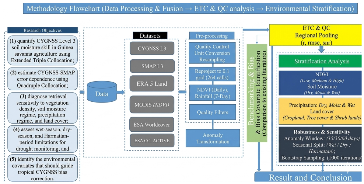
The objectives are to: (1) quantify Extended Triple Collocation (ETC)-derived CYGNSS Level 3 soil moisture performance in Guinea savanna agriculture as a latent statistical estimate rather than direct ground validation; (2) test whether the SMAP-inclusive collocation configuration produces a higher CYGNSS estimate than a SMAP-independent configuration using covariance-pathway Quadruple Collocation (QC); (3) diagnose retrieval sensitivity to vegetation density, soil moisture regime, precipitation regime, and land cover; (4) assess wet-season, dry-season, and Harmattan-period limitations using convergence, variance, covariance, and condition-number diagnostics; and (5) identify the environmental covariates that should guide future tropical CYGNSS bias correction.

2. Materials and Methods

2.1. Study Area

Benue State is located in the North Central geopolitical zone of Nigeria between approximately 6.44°N and 8.14°N, and 7.55°E and 9.94°E. It covers about 34,059 km² across 23 Local Government Areas. Elevation ranges from low-lying floodplains near the Benue and Katsina-Ala Rivers to upland areas approaching 450 m above sea level [28]. The state lies fully within the CYGNSS observation domain.

The climate is tropical savanna under the Koppen Aw classification [29]. Rainfall is strongly seasonal. The wet season generally extends from April to October, while the dry season extends from November to March under northeasterly Harmattan winds [30,31]. Annual rainfall commonly ranges from about 1200 to 1500 mm, with peak rainfall between July and September [7,31]. This seasonal cycle produces large soil moisture changes and provides a useful dynamic range for satellite evaluation.

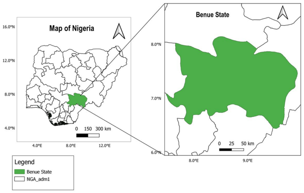
The land surface is an agricultural mosaic. ESA WorldCover 2021 indicates that cropland accounts for 46.6% of the study domain, tree cover for 29.2%, and shrubland or grassland for 24.2%. This mixture is important because GNSS-R retrievals respond differently over seasonal crop canopies, open savanna, and persistent woodland. The absence of a dense in situ soil moisture network makes Benue State an appropriate setting for collocation-based validation. Figure 1 shows the study area and the intended analysis-grid context.

2.2. Datasets

Six datasets were used for collocation analysis, environmental stratification, and robustness testing. They include one GNSS-R soil moisture product, one passive microwave product, one land surface reanalysis, one vegetation index product, one active microwave soil moisture product, and one land-cover product (

Table 1. Datasets used in the study.

Dataset	Source	Resolution	Period	Role in Analysis
CYGNSS L3 Soil Moisture v3.2	NASA PO.DAAC	0.1°	2021–2023	Target GNSS-R soil moisture product evaluated in all ETC and stratified performance analyses.
SMAP Enhanced L3 v6	NASA NSIDC	9 km	2021–2023	Passive microwave soil moisture product used in the primary ETC triplet and as the SMAP-inclusive benchmark.
ERA5-Land	ECMWF CDS	0.1°	2021–2023	Land surface model product and source of precipitation data used as the third member of the primary ETC triplet.
MODIS MOD13Q1 NDVI v61	NASA LP DAAC	250 m	2021–2023	Vegetation-density covariate used to stratify CYGNSS retrieval performance.
ESA CCI ACTIVE v09.2	CEDA and H-SAF	0.25°	2021–2023	Active microwave soil moisture product used as the fourth, structurally distinct product in Quadruple Collocation.
ESA WorldCover 2021 v200	ESA and Copernicus	10 m	Static	Land-cover product used to assign dominant cropland, shrubland or grassland, and tree-cover classes.

Abbreviations: CYGNSS, Cyclone Global Navigation Satellite System; L3, Level 3; SMAP, Soil Moisture Active Passive; ERA5-Land, fifth-generation land reanalysis; MODIS, Moderate Resolution Imaging Spectroradiometer; NDVI, Normalized Difference Vegetation Index; ESA CCI, European Space Agency Climate Change Initiative; GNSS-R, Global Navigation Satellite System Reflectometry; ETC, Extended Triple Collocation.

).

CYGNSS Level 3 Soil Moisture v3.2 was obtained from NASA PO.DAAC. The product provides volumetric soil moisture estimates derived from calibrated GNSS-R surface reflectivity through SMAP-trained regression relationships [21]. Only retrievals with uncertainty below 0.1 m³ m⁻³ were retained.

SMAP Enhanced Level 3 v6 was obtained from NASA NSIDC. SMAP measures L-band brightness temperature at 1.41 GHz and provides surface soil moisture estimates for the upper few centimeters of the soil column [18,20,32]. Descending morning overpasses were used because they are generally less affected by thermal disequilibrium than afternoon retrievals.

ERA5-Land was obtained from the ECMWF Climate Data Store. It provides hourly land surface variables at 0.1° resolution from an offline land surface model driven by ERA5 atmospheric forcing [33]. The 0 to 7 cm soil layer was used for surface soil moisture, and seven-day accumulated precipitation was used for stratification.

Moderate Resolution Imaging Spectroradiometer (MODIS) MOD13Q1 Normalized Difference Vegetation Index (NDVI) was used to characterize vegetation density [34]. The European Space Agency Climate Change Initiative (ESA CCI) ACTIVE v09.2 product was used as the fourth product for Quadruple Collocation. It is derived from active microwave scatterometer observations and is structurally distinct from CYGNSS and SMAP in sensor physics, frequency band, and retrieval chain [14,35]. This structural distinction does not imply perfect error independence, because land-surface products can still share indirect dependencies through vegetation state, topography, land-cover classification, soil texture, or common hydrometeorological forcing. ESA WorldCover 2021 was used to assign the dominant land cover class in each grid cell [36].

2.3. Spatial and Temporal Harmonization

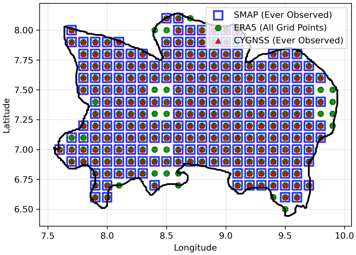
All datasets were harmonized to a common 0.1° grid with 264 spatial locations over Benue State. This grid matches the native resolution of ERA5-Land and the finer CYGNSS Level 3 gridding option. ERA5-Land fields were interpolated to the target grid. SMAP observations were averaged within 0.05° of each grid point. CYGNSS observations were assigned by nearest-neighbor matching within the same radius. MODIS NDVI was spatially averaged within each grid cell.

Temporal harmonization used daily matching. CYGNSS and SMAP observations were paired with ERA5-Land daily mean surface soil moisture. A valid ETC triplet required simultaneous CYGNSS, SMAP, and ERA5-Land observations after all quality filters. A valid quadruplet additionally required ESA CCI ACTIVE. The analysis period covered 2021 to 2023, equivalent to 1095 daily time steps. The harmonized analysis grid and the spatial coverage of the primary collocation products are shown in Figure 2.

2.4. Soil Moisture Anomaly Calculation

Collocation analysis was applied to soil moisture anomalies rather than raw values. This reduces systematic offsets among products and focuses the analysis on temporally varying departures from the local background state [14]. Anomaly processing is also useful for improving approximate linearity among products with different climatologies and dynamic ranges. The trade-off is that moving-window anomalies suppress part of the slowly varying seasonal component and may smooth very abrupt flash-drought onset or rapid post-rainfall recovery. The analysis should therefore be interpreted as a sub-seasonal anomaly-tracking assessment rather than a direct test of instantaneous soil moisture retrieval accuracy.

For each product and grid cell, anomalies were calculated using a 31-day centered moving window. This definition matches the implemented ETC and QC processing code used for all primary results. Let $x_{i,t}$ denote soil moisture from product i at time t. The moving-window mean and anomaly are

$${\overline{x}}_{i,t}^{\left(31\right)}={\displaystyle \frac{1}{n_{i,t}}}{\displaystyle \sum _{k=-15}^{15}}{x}_{i,t+k},x_{i,t}^{\prime }=x_{i,t}-{\overline{x}}_{i,t}^{\left(31\right)},$$

(1)

where $n_{i,t}$ is the number of valid observations for product i within the window from day $t-15$ to day $t+15$. The window was applied continuously across the 2021–2023 record without calendar-year restriction. Sensitivity tests using shorter and longer anomaly windows are reported in Section 3.8 and Appendix A.1.

2.5. Extended Triple Collocation

Extended Triple Collocation estimates error variance and correlation with an unknown latent signal without requiring ground truth [12,13]. These estimates are model-derived statistical quantities and should not be interpreted as direct validation against an absolute physical truth. Each product is represented as an affine function of the latent soil moisture anomaly:

$$x_i={\alpha }_i+{\beta }_i\theta +{\epsilon }_i,$$

(2)

where $x_i$ is the anomaly from product i, $\theta$ is the latent soil moisture anomaly signal, ${\alpha }_i$ is an intercept, ${\beta }_i$ is a scaling coefficient, and ${\epsilon }_i$ is a zero-mean random error. The standard assumptions are linearity, stationarity, error orthogonality with the latent signal, and zero error cross-correlation among products [13,14].

For a triplet $(X,Y,Z)$, the error variance of product X is estimated as

$${\sigma }_{{\epsilon }_X}^2={\sigma }_X^2-{\displaystyle \frac{{\sigma }_{XY}{\sigma }_{XZ}}{{\sigma }_{YZ}}},$$

(3)

with analogous expressions for Y and Z. The square root of this quantity is reported as the ETC-derived estimated error standard deviation, not as a ground-truth estimated error standard deviation. Correlation with the latent signal is estimated as

$${\rho }_{X,\theta }=\sqrt{1-{\displaystyle \frac{{\sigma }_{{\epsilon }_X}^2}{{\sigma }_X^2}}}.$$

(4)

The positive root is used because soil moisture products should increase with the latent soil moisture signal. Signal-to-noise ratio (SNR) was expressed in decibels as

$${\mathrm{SNR}}_X=10{log}_{10}\left({\displaystyle \frac{{\sigma }_X^2-{\sigma }_{{\epsilon }_X}^2}{{\sigma }_{{\epsilon }_X}^2}}\right).$$

(5)

Positive SNR indicates that the ETC-estimated signal variance exceeds the estimated error variance. Negative SNR indicates that, within the adopted collocation model, the estimated error variance exceeds the estimated signal variance. It does not imply that the product contains no soil moisture information.

2.6. Quadruple Collocation

Quadruple Collocation (QC) was used to test whether the standard CYGNSS–SMAP–ERA5-Land ETC triplet is affected by the SMAP-related calibration structure of the CYGNSS Level 3 soil moisture product. The concern is structural rather than purely empirical. CYGNSS Level 3 soil moisture is generated using regression relationships trained against SMAP observations [21]. Therefore, a triplet that includes both CYGNSS and SMAP may be less conservative than a triplet in which CYGNSS is evaluated without SMAP. QC was introduced to examine this issue by adding a fourth soil moisture product, ESA CCI ACTIVE, that is structurally distinct from both CYGNSS and SMAP in sensor physics, frequency band, and retrieval chain. The four-product collocation model is written as

$$x_i={\alpha }_i+{\beta }_i\theta +{\epsilon }_i,i\in \{X,Y,Z,W\},$$

(6)

where X, Y, Z, and W denote CYGNSS, SMAP, ERA5-Land, and ESA CCI ACTIVE, respectively. Here, $x_i$ is the anomaly from product i, $\theta$ is the unknown latent soil moisture anomaly signal, ${\alpha }_i$ is an intercept, ${\beta }_i$ is a linear sensitivity coefficient, and ${\epsilon }_i$ is the random error term. The formulation allows a possible cross-error covariance between CYGNSS and SMAP because CYGNSS Level 3 is trained using SMAP. All other direct retrieval-chain error covariances are assumed to be zero. Under this structure, the covariance matrix is

$$\mathbf{C}=\left[\begin{array}{cccc}{\beta }_X^2{\sigma }_{\theta }^2+{\sigma }_{{\epsilon }_X}^2& {\beta }_X{\beta }_Y{\sigma }_{\theta }^2+{\sigma }_{{\epsilon }_X{\epsilon }_Y}& {\beta }_X{\beta }_Z{\sigma }_{\theta }^2& {\beta }_X{\beta }_W{\sigma }_{\theta }^2\\ {\beta }_X{\beta }_Y{\sigma }_{\theta }^2+{\sigma }_{{\epsilon }_X{\epsilon }_Y}& {\beta }_Y^2{\sigma }_{\theta }^2+{\sigma }_{{\epsilon }_Y}^2& {\beta }_Y{\beta }_Z{\sigma }_{\theta }^2& {\beta }_Y{\beta }_W{\sigma }_{\theta }^2\\ {\beta }_X{\beta }_Z{\sigma }_{\theta }^2& {\beta }_Y{\beta }_Z{\sigma }_{\theta }^2& {\beta }_Z^2{\sigma }_{\theta }^2+{\sigma }_{{\epsilon }_Z}^2& {\beta }_Z{\beta }_W{\sigma }_{\theta }^2\\ {\beta }_X{\beta }_W{\sigma }_{\theta }^2& {\beta }_Y{\beta }_W{\sigma }_{\theta }^2& {\beta }_Z{\beta }_W{\sigma }_{\theta }^2& {\beta }_W^2{\sigma }_{\theta }^2+{\sigma }_{{\epsilon }_W}^2\end{array}\right].$$

(7)

In Equation (7), ${\sigma }_{{\epsilon }_X{\epsilon }_Y}$ is the possible CYGNSS–SMAP cross-error covariance. If ${\sigma }_{{\epsilon }_X{\epsilon }_Y}=0$, the CYGNSS–SMAP pair satisfies the standard ETC independence assumption. If it differs from zero, the observed CYGNSS–SMAP covariance contains both a shared latent-signal component and a shared-error component. After anomaly centering, the QC estimator separates these two components by estimating the latent-signal contribution to the observed CYGNSS–SMAP covariance through two alternative covariance pathways that are algebraically equivalent under the ideal QC assumptions. Since Z and W are assumed not to share direct retrieval-chain errors with the CYGNSS–SMAP pair,

$${\sigma }_{XZ}={\beta }_X{\beta }_Z{\sigma }_{\theta }^2,{\sigma }_{YW}={\beta }_Y{\beta }_W{\sigma }_{\theta }^2,{\sigma }_{ZW}={\beta }_Z{\beta }_W{\sigma }_{\theta }^2.$$

(8)

Therefore,

$${\displaystyle \frac{{\sigma }_{XZ}{\sigma }_{YW}}{{\sigma }_{ZW}}}={\displaystyle \frac{\left({\beta }_X{\beta }_Z{\sigma }_{\theta }^2\right)\left({\beta }_Y{\beta }_W{\sigma }_{\theta }^2\right)}{{\beta }_Z{\beta }_W{\sigma }_{\theta }^2}}={\beta }_X{\beta }_Y{\sigma }_{\theta }^2.$$

(9)

The right-hand side of Equation (9) is the latent-signal component of the CYGNSS–SMAP covariance. A second pathway gives the same target quantity:

$${\displaystyle \frac{{\sigma }_{XW}{\sigma }_{YZ}}{{\sigma }_{ZW}}}={\displaystyle \frac{\left({\beta }_X{\beta }_W{\sigma }_{\theta }^2\right)\left({\beta }_Y{\beta }_Z{\sigma }_{\theta }^2\right)}{{\beta }_Z{\beta }_W{\sigma }_{\theta }^2}}={\beta }_X{\beta }_Y{\sigma }_{\theta }^2.$$

(10)

The two empirical signal-covariance estimates are therefore

$${\widehat{cov}}_{\mathrm{sig},1}(X,Y)={\displaystyle \frac{{\sigma }_{XZ}{\sigma }_{YW}}{{\sigma }_{ZW}}},{\widehat{cov}}_{\mathrm{sig},2}(X,Y)={\displaystyle \frac{{\sigma }_{XW}{\sigma }_{YZ}}{{\sigma }_{ZW}}}.$$

(11)

Because real satellite products do not satisfy the ideal QC assumptions exactly, the mean of the two pathways was used as the diagnostic estimate of the latent-signal contribution:

$${\widehat{cov}}_{\mathrm{sig}}(X,Y)={\displaystyle \frac{1}{2}}\left[{\widehat{cov}}_{\mathrm{sig},1}(X,Y)+{\widehat{cov}}_{\mathrm{sig},2}(X,Y)\right].$$

(12)

The observed CYGNSS–SMAP covariance can then be decomposed as

$${\sigma }_{XY}={\beta }_X{\beta }_Y{\sigma }_{\theta }^2+{\sigma }_{{\epsilon }_X{\epsilon }_Y}.$$

(13)

Substituting the pathway estimate of the latent-signal covariance into Equation (13) gives the CYGNSS–SMAP cross-error covariance estimator:

$$\widehat{cov}({\epsilon }_X,{\epsilon }_Y)={\sigma }_{XY}-{\widehat{cov}}_{\mathrm{sig}}(X,Y).$$

(14)

For the corresponding cross-error correlation, the CYGNSS and SMAP error variances were estimated from the same covariance-pathway framework as

$${\widehat{\sigma }}_{{\epsilon }_X}^2={\sigma }_X^2-{\displaystyle \frac{{\sigma }_{XZ}{\sigma }_{XW}}{{\sigma }_{ZW}}},{\widehat{\sigma }}_{{\epsilon }_Y}^2={\sigma }_Y^2-{\displaystyle \frac{{\sigma }_{YZ}{\sigma }_{YW}}{{\sigma }_{ZW}}}.$$

(15)

The CYGNSS–SMAP cross-error correlation is then

$$r_{\epsilon ,\mathrm{CYGNSS},\mathrm{SMAP}}={\displaystyle \frac{\widehat{cov}\left({\epsilon }_{\mathrm{CYGNSS}},{\epsilon }_{\mathrm{SMAP}}\right)}{{\widehat{\sigma }}_{\epsilon ,\mathrm{CYGNSS}}{\widehat{\sigma }}_{\epsilon ,\mathrm{SMAP}}}}.$$

(16)

The QC estimator is identifiable only under several conditions. The four products must be approximately linearly related to the same latent soil moisture anomaly signal; the covariance terms ${\sigma }_{XZ}$, ${\sigma }_{XW}$, ${\sigma }_{YZ}$, ${\sigma }_{YW}$, and ${\sigma }_{ZW}$ must be non-zero and physically consistent; the latent anomaly variance must not be negligible; and the covariance matrix must be sufficiently well conditioned. The method also requires that ERA5-Land and ESA CCI ACTIVE do not share direct retrieval-chain errors with the CYGNSS–SMAP pair. This last condition is weaker than perfect independence. Residual indirect dependence may still arise through shared land-surface controls, vegetation state, topography, soil texture, precipitation forcing, static land-cover information, or representativeness effects caused by mismatched spatial footprints. These possible indirect pathways are therefore treated as limitations when interpreting the QC result. Bootstrap resampling with 1000 iterations was used to estimate confidence intervals for the cross-error covariance and cross-error correlation. The QC analysis was used in two complementary ways: first, to test whether direct CYGNSS–SMAP cross-error correlation was detectable; and second, to compare the CYGNSS estimate from a SMAP-inclusive triplet with the estimate from a SMAP-independent triplet. The SMAP-independent estimate was retained as the conservative benchmark for interpreting CYGNSS performance in the study region.

2.7. Environmental Stratification

CYGNSS performance was stratified by four environmental controls that influence GNSS-R soil moisture retrievals: vegetation density, soil moisture regime, precipitation regime, and land cover class (

Table 2. Environmental stratification classes used in the analysis.

Variable	Class	Range	Physical Rationale
NDVI	Low	0.0 to 0.3	Sparse canopy and limited vegetation attenuation.
NDVI	Medium	0.3 to 0.6	Active crop or savanna growth with moderate attenuation.
NDVI	High	0.6 to 1.0	Dense canopy and stronger L-band attenuation.
Soil moisture	Dry	0.00 to 0.15 ${\mathrm{m}}^3{\mathrm{m}}^{-3}$	Drought-relevant conditions and reduced dielectric sensitivity.
Soil moisture	Medium	0.15 to 0.30 ${\mathrm{m}}^3{\mathrm{m}}^{-3}$	Intermediate moisture and stronger dielectric sensitivity.
Soil moisture	Wet	0.30 to 0.60 ${\mathrm{m}}^3{\mathrm{m}}^{-3}$	Possible saturation, ponding, or reduced contrast.
Precipitation	Low	0 to 10 mm week−1	Limited recent wetting.
Precipitation	Moderate	10 to 30 mm week−1	Active wetting and drying with limited ponding risk.
Precipitation	High	>30 mm week−1	Possible surface water and wet-condition interference.
Land cover	Cropland	Majority class	Seasonal agricultural canopy.
Land cover	Shrubland/grassland	Majority class	Open savanna surface.
Land cover	Tree cover	Majority class	Persistent woody canopy.

). Vegetation density was represented by MODIS NDVI. Soil moisture regime was defined using ERA5-Land surface soil moisture. Precipitation regime was represented by seven-day accumulated ERA5-Land precipitation. Land cover was assigned from ESA WorldCover 2021. The thresholds were selected to represent sparse, moderate, and dense vegetation; dry, intermediate, and wet soil states; and limited, moderate, and high recent rainfall conditions. To test whether the conclusions depended on the exact boundary values, alternative threshold sets were evaluated for NDVI, soil moisture, and precipitation in the robustness analysis.

2.8. Uncertainty and Robustness Assessment

Uncertainty was quantified using bootstrap resampling, pairwise significance tests, sensitivity analysis, convergence diagnostics, and spatial diagnostics. Bootstrap confidence intervals used 1000 iterations. Pairwise environmental contrasts were considered significant when the 95% confidence interval of the difference excluded zero.

Robustness tests examined anomaly-window sensitivity; random subsampling at 75%, 50%, and 25% of valid triplets; bootstrap seed independence; random, spatial, and temporal cross-validation; threshold sensitivity for environmental stratification; wet-season and dry-season convergence; covariance condition numbers; variance-normalized ETC; and spatial autocorrelation correction. Moran’s I and the Clifford effective sample size correction were used to assess spatial dependence among location-level ETC estimates [37]. Sub-grid representativeness was assessed using ESA WorldCover-derived Shannon entropy, Simpson’s diversity index, and dominant-class proportion within each 0.1° grid cell. The complete processing and evaluation sequence is summarized in Figure 3, with detailed diagnostic tables placed in Appendix A.

All data processing, collocation analysis, statistical evaluation, and visualization were performed using Python (version 3.13.4) in the Jupyter Notebook environment (Project Jupyter, https://jupyter.org/, accessed on 25 July 2026). Standard Python scientific, statistical, geospatial, and plotting libraries were used. Maps were prepared using QGIS (https://qgis.org/, accessed on 25 July 2026).

3. Results

3.1. Collocated Data Availability and Sampling Characteristics

The full space–time domain contained 289,080 possible daily grid-time slots. After quality screening, CYGNSS provided 56,947 valid observations, equal to 19.7% of the full domain. SMAP provided 189,413 valid observations, equal to 65.5%. ERA5-Land provided complete coverage by definition. The final ETC dataset contained 40,003 valid CYGNSS–SMAP–ERA5-Land triplets. Quadruple Collocation used 39,906 valid four-product records (

Table 3. Sample flow and collocation summary for the 2021 to 2023 analysis period.

Stage	N	Description
Full space–time slots	289,080	264 grid locations multiplied by 1095 days.
Valid CYGNSS observations	56,947	19.7% of all slots after quality filtering.
Valid SMAP observations	189,413	65.5% of the full domain.
Valid ERA5-Land observations	289,080	100% continuous reanalysis coverage.
Valid triplets	40,003	Primary ETC dataset.
Wet-season triplets	28,015	April to October.
Dry-season triplets	11,988	November to March.
Valid quadruplets	39,906	Dataset used for Quadruple Collocation.

). Wet-season triplets accounted for 70.0% of the valid ETC sample, while dry-season triplets accounted for 30.0%.

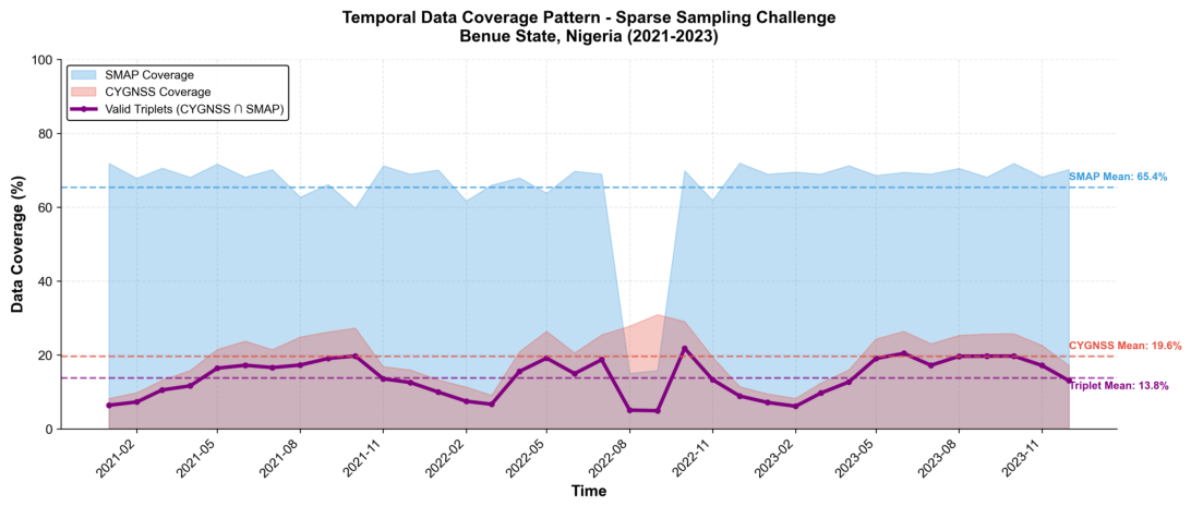
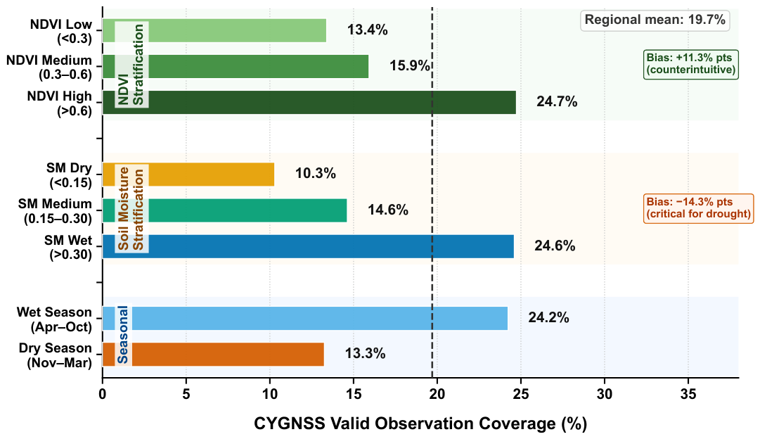
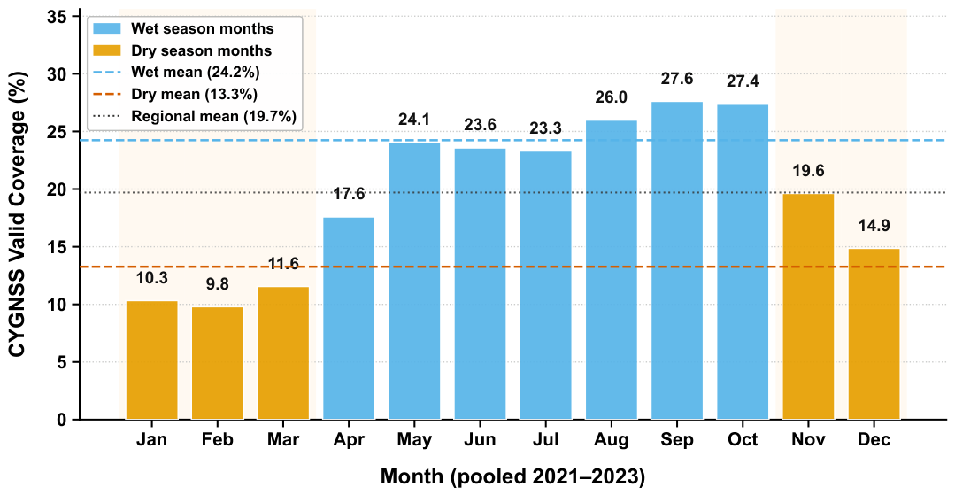
CYGNSS sampling was not environmentally uniform. Figure 4 shows that SMAP maintained much higher temporal coverage than CYGNSS throughout 2021 to 2023. Mean SMAP coverage was about 65.4%, while mean CYGNSS coverage was about 19.6%. The resulting valid CYGNSS–SMAP triplet coverage averaged only 13.8%, showing that the ETC sample was constrained mainly by CYGNSS availability.

This temporal sparsity also varied seasonally. Valid CYGNSS coverage was higher during the wet season than during the dry season, with 24.2% coverage during April to October and 13.3% during November to March. The environmental sampling pattern is shown in Figure 5, while the monthly coverage pattern is shown in Figure 6. Together, these figures show that CYGNSS coverage was lower under dry soil conditions and during Harmattan months. This means that the dry stratum is likely weighted toward transitional dry cases rather than the most severe Harmattan dryness.

3.2. Regional ETC Performance of CYGNSS, SMAP, and ERA5-Land

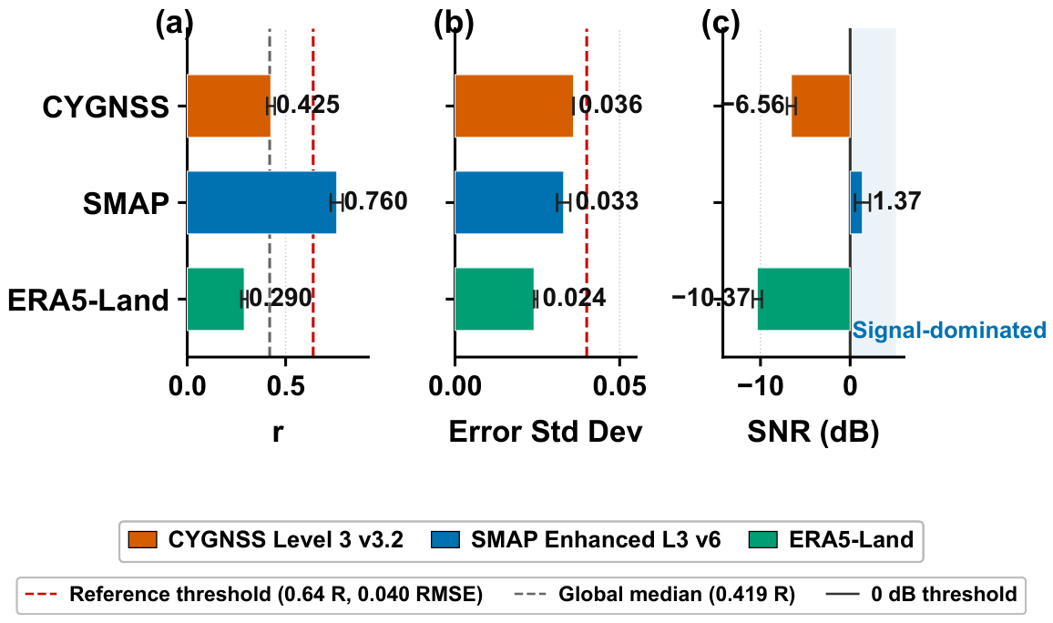
Regional ETC results show clear differences among the three primary products (

Table 4. Regional ETC performance for the primary CYGNSS–SMAP–ERA5-Land configuration.

Product	Estimated Error SD (${\mathbf{m}}^{\mathbf{3}}{\mathbf{m}}^{\mathbf{-}\mathbf{3}}$)	r	SNR (dB)	N
CYGNSS	0.036	0.425	−6.56	40,003
SMAP	0.033	0.760	+1.37	40,003
ERA5-Land	0.024	0.290	−10.37	40,003

). These quantities are collocation-derived latent statistical estimates rather than direct ground-validation metrics. SMAP had the strongest overall performance, with $r=0.760$ (95% confidence interval (CI) [0.729, 0.790]), an estimated error standard deviation of $0.033{\mathrm{m}}^3{\mathrm{m}}^{-3}$ (95% CI [0.031, 0.035]), and SNR of $+1.37$ dB (95% CI [+0.544, +2.209]). The positive SNR indicates that, within the ETC model, the estimated signal variance exceeded the estimated error variance for SMAP.

CYGNSS showed measurable but more limited anomaly-tracking skill. Its SMAP-inclusive ETC correlation was $r=0.425$ (95% CI [0.406, 0.445]), with an estimated error standard deviation of $0.036{\mathrm{m}}^3{\mathrm{m}}^{-3}$ (95% CI [0.036, 0.036]) and SNR of $-6.56$ dB (95% CI [−7.046, −6.072]). The negative SNR indicates that the ETC-estimated error variance exceeded the estimated signal variance for CYGNSS under the primary triplet configuration. This does not imply that CYGNSS contains no soil moisture information, but it does indicate limited reliability for direct anomaly tracking without environmental correction.

ERA5-Land had the lowest estimated error standard deviation, $0.024{\mathrm{m}}^3{\mathrm{m}}^{-3}$ (95% CI [0.024, 0.025]), but also the weakest estimated correlation with the latent anomaly signal, $r=0.290$ (95% CI [0.275, 0.306]), and the most negative SNR, $-10.37$ dB (95% CI [−10.870, −9.851]). This pattern shows that a low estimated error spread does not necessarily imply stronger anomaly tracking. Table 4 reports the ETC metrics and confidence intervals, while Figure 7 visualizes the regional contrasts among CYGNSS, SMAP, and ERA5-Land.

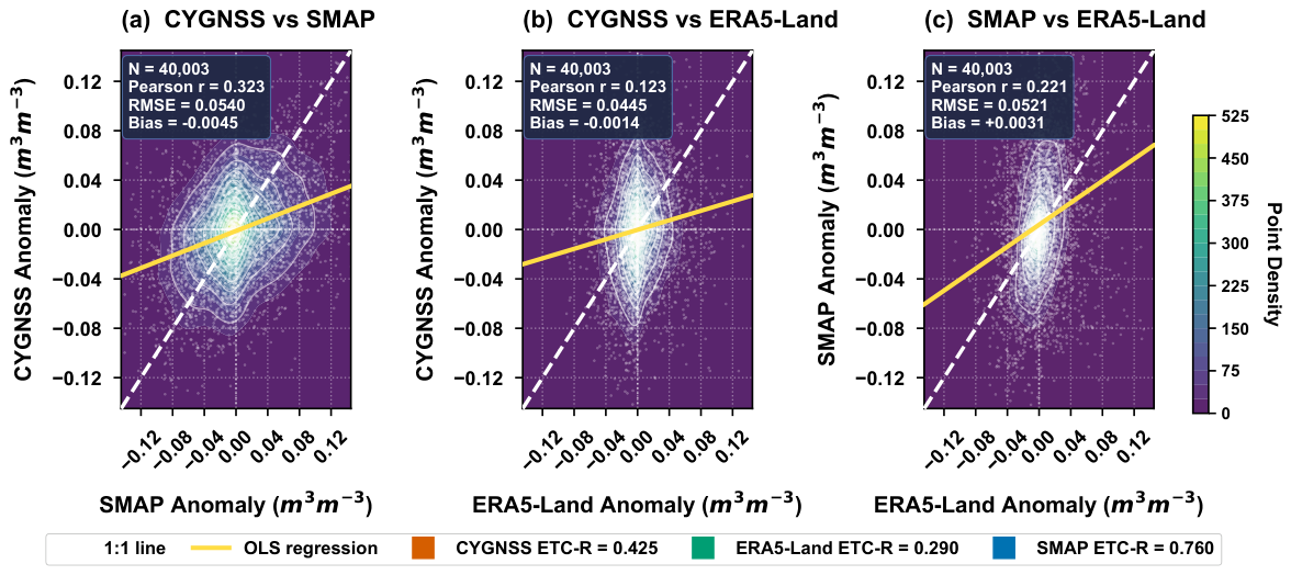
The pairwise anomaly structure underlying the ETC covariance decomposition is shown in Figure 8.

The regional result establishes two points. CYGNSS contains measurable soil moisture anomaly information in Guinea savanna agriculture, but the negative ETC-derived SNR indicates that the estimated error variance exceeds the estimated signal variance within the adopted collocation model. This does not mean that CYGNSS is uninformative, but it does indicate limited reliability for direct anomaly tracking without environmental correction.

3.3. Quadruple Collocation and SMAP-Inclusive Configuration Sensitivity

The covariance-pathway QC estimator defined in Section 2.6 was applied to the common four-product anomaly sample to separate the observed CYGNSS–SMAP covariance into an estimated shared-signal component and a residual cross-error component. The covariance-pathway QC analysis did not detect statistically significant direct CYGNSS–SMAP error correlation. In the common four-product sample of 39,906 quadruplets, the estimated CYGNSS–SMAP cross-error covariance was $0.000001$, with a 95% bootstrap confidence interval of $[-0.000055,0.000058]$. The corresponding cross-error correlation was $r_{\epsilon }=0.0007$, with a 95% confidence interval of $[-0.0270,0.0283]$. Because this interval includes zero, the analysis does not support a claim of significant direct CYGNSS–SMAP error correlation in the Benue State anomaly dataset.

The triplet sensitivity analysis nevertheless showed that the SMAP-inclusive configuration gave a modestly higher CYGNSS estimate than the SMAP-independent configuration. In the common quadruplet sample, the CYGNSS–SMAP–ERA5-Land triplet produced $r=0.423$, while the CYGNSS–ERA5-Land–ESA CCI ACTIVE triplet produced $r=0.386$. The difference of $\Delta r=0.0368$ indicates modest configuration-dependent inflation. The SMAP-independent estimate is therefore retained as the conservative baseline for interpreting CYGNSS performance. This interpretation is more cautious than attributing the difference to a large direct CYGNSS–SMAP error covariance. The complete ETC triplet comparisons and QC diagnostics are summarized in

Table 5. CYGNSS and SMAP estimates from ETC triplet configurations and covariance-pathway QC diagnostics. Correlations are ETC-derived latent estimates, not direct ground-validation coefficients.

Analysis	Product Configuration	Quantity Reported	Estimate	Interpretation
T1	CYGNSS, SMAP, ERA5-Land	CYGNSS correlation with latent anomaly signal	$r=0.423$ [0.404, 0.443]	SMAP-inclusive estimate in the common quadruplet sample.
T2	CYGNSS, SMAP, ESA CCI ACTIVE	CYGNSS correlation with latent anomaly signal	$r=0.387$ [0.376, 0.399]	Diagnostic configuration replacing ERA5-Land with active microwave observations.
T3	CYGNSS, ERA5-Land, ESA CCI ACTIVE	CYGNSS correlation with latent anomaly signal	$r=0.386$ [0.366, 0.405]	SMAP-independent conservative baseline.
T4	SMAP, ERA5-Land, ESA CCI ACTIVE	SMAP correlation with latent anomaly signal	$r=0.756$ [0.734, 0.778]	Reference check showing strong SMAP performance in a CYGNSS-free triplet.
QC	CYGNSS, SMAP, ERA5-Land, ESA CCI ACTIVE	CYGNSS–SMAP cross-error correlation	$r_{\epsilon }=0.0007$ [−0.0270, 0.0283]	No statistically significant direct error correlation detected.

.

The QC result changes the interpretation of the SMAP-related issue. The main concern is not a large detected CYGNSS–SMAP error correlation, but the fact that the SMAP-inclusive configuration gives a slightly higher CYGNSS estimate than the SMAP-independent configuration. This supports using the SMAP-independent triplet as the conservative benchmark, while acknowledging that the observed difference may reflect a combination of product sensitivity, sampling, scaling, and residual structural dependence.

3.4. Environmental Controls on CYGNSS Performance

Environmental stratification shows that regional performance is not uniform. CYGNSS skill varies with vegetation density, soil moisture state, recent precipitation, and land cover (

Table 6. CYGNSS ETC performance stratified by environmental controls.

Variable	Class	N	Estimated Error SD (${\mathbf{m}}^{\mathbf{3}}{\mathbf{m}}^{\mathbf{-}\mathbf{3}}$)	r	SNR (dB)
NDVI	Low	2058	0.036	0.510	−4.55
NDVI	Medium	15,643	0.038	0.443	−6.12
NDVI	High	22,038	0.034	0.408	−7.00
Soil moisture	Dry	11,198	0.039	0.331	−9.11
Soil moisture	Medium	17,985	0.033	0.481	−5.21
Soil moisture	Wet	10,557	0.037	0.336	−8.95
Precipitation	Low	9663	0.037	0.366	−8.10
Precipitation	Moderate	2660	0.036	0.630	−1.83
Precipitation	High	15,037	0.037	0.427	−6.51
Land cover	Cropland	19,708	0.035	0.447	−6.02
Land cover	Shrubland/grassland	10,578	0.037	0.455	−5.83
Land cover	Tree cover	9717	0.036	0.342	−8.79

). These patterns explain why a single regional value cannot fully describe tropical retrieval performance. Pairwise bootstrap tests for the environmental contrasts are reported in Appendix A.3 and

Table A5. Pairwise bootstrap significance tests across environmental strata. Significance is declared when the 95% bootstrap confidence interval of the pairwise difference, $r_A-r_B$, excludes zero. The confidence intervals report bootstrapped difference intervals, not individual stratum correlation intervals.

Stratification	Comparison	${\mathit{r}}_{\mathit{A}}$	${\mathit{r}}_{\mathit{B}}$	CI Lower	CI Upper	Significant
NDVI	Low vs. medium	0.510	0.443	−0.064	+0.259	No
NDVI	Low vs. high	0.510	0.408	−0.022	+0.297	No
NDVI	Medium vs. high	0.443	0.408	−0.009	+0.077	No
Soil moisture	Dry vs. medium	0.331	0.481	−0.204	−0.097	Yes
Soil moisture	Dry vs. wet	0.331	0.336	−0.055	+0.054	No
Soil moisture	Medium vs. wet	0.481	0.336	+0.092	+0.197	Yes
Precipitation	Low vs. moderate	0.366	0.630	−0.358	−0.173	Yes
Precipitation	Low vs. high	0.366	0.427	−0.098	+0.005	No
Precipitation	Moderate vs. high	0.630	0.427	+0.141	+0.307	Yes
Land cover	Cropland vs. tree cover	0.447	0.342	+0.061	+0.153	Yes
Land cover	Cropland vs. shrubland or grassland	0.447	0.455	−0.057	+0.040	No
Land cover	Shrubland or grassland vs. tree cover	0.455	0.342	+0.059	+0.167	Yes

.

3.4.1. Vegetation Density

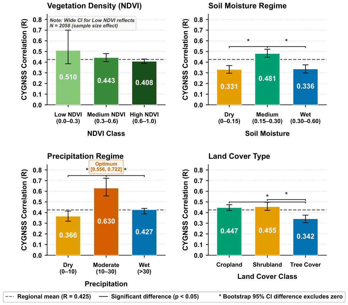
CYGNSS performance declined with increasing NDVI. Correlation decreased from $r=0.510$ under low NDVI to $r=0.443$ under medium NDVI and $r=0.408$ under high NDVI. SNR also declined from $-4.55$ dB to $-7.00$ dB. This monotonic pattern is physically consistent with increasing canopy attenuation and non-soil scattering contributions under dense vegetation [17,38].

3.4.2. Soil Moisture Regime

Soil moisture regime produced the clearest operational pattern. CYGNSS performed worst under dry soils, where $r=0.331$ and SNR was $-9.11$ dB. Performance improved in the medium soil moisture range, where $r=0.481$. It decreased again under wet conditions, where $r=0.336$.

The dry-condition weakness is operationally important. It occurs when early detection of agricultural drought stress is most valuable. It may also be optimistic because severe dry-season conditions are under-sampled by valid CYGNSS retrievals.

3.4.3. Precipitation Regime

The precipitation stratification shows a distinct performance optimum under moderate recent rainfall. CYGNSS achieved $r=0.630$ under 10 to 30 mm week⁻¹, compared with $r=0.366$ under low precipitation and $r=0.427$ under high precipitation. Moderate rainfall likely produces detectable wetting and drying dynamics without the surface water interference associated with heavy rainfall [39].

3.4.4. Land Cover Class

Land cover stratification separates agricultural and open savanna surfaces from persistent tree cover. Cropland yielded $r=0.447$, and shrubland or grassland yielded $r=0.455$. Tree cover performed substantially worse at $r=0.342$. This result shows that CYGNSS is more promising over agricultural and open savanna surfaces than over persistent woodland. Table 6 reports the full stratified performance matrix, and Figure 9 summarizes the environmental contrasts visually.

3.5. Threshold Sensitivity of Environmental Stratification

Threshold sensitivity tests were conducted to verify that the environmental conclusions were not artifacts of the selected class boundaries. The tests used the same collocated anomaly dataset as the stratified ETC analysis after applying the environmental covariate filters, yielding 39,740 valid triplets. For each continuous stratification variable, the original boundary pair and four alternative boundary pairs were tested. The exact threshold sets, sample sizes, and class-specific correlations are reported in Appendix A.2, while the main interpretation is summarized here.

For NDVI, the original boundaries were 0.30 and 0.60. Alternative boundaries were 0.20/0.55, 0.25/0.60, 0.35/0.70, and 0.20/0.65. The original thresholds produced a declining vegetation-density pattern: low NDVI gave $r=0.5096$, medium NDVI gave $r=0.4432$, and high NDVI gave $r=0.4077$. Across the alternative tests, the medium-NDVI class remained stable, with r values between 0.4325 and 0.4502, while the high-NDVI class remained lower, between 0.3644 and 0.4109. The low-NDVI class was more sensitive because it had fewer observations and was retained as a stable ETC stratum in only two threshold runs. Therefore, the NDVI interpretation is not that all boundaries produce the same ranking, but that dense vegetation consistently limits CYGNSS performance relative to the medium vegetation regime.

For soil moisture, the original boundaries were 0.15 and $0.30{\mathrm{m}}^3{\mathrm{m}}^{-3}$. Alternative boundaries were 0.10/0.25, 0.18/0.35, 0.12/0.28, and $0.20/0.40{\mathrm{m}}^3{\mathrm{m}}^{-3}$. The medium soil moisture class was the most stable high-performing regime. It produced $r=0.4810$ under the original thresholds and remained highest in four of the five tested boundary sets. Dry-soil performance remained low, ranging from $r=0.3128$ to $r=0.3906$, while wet-soil performance ranged from $r=0.3360$ to $r=0.4212$. The only case where the wet class ranked highest was the $0.20/0.40{\mathrm{m}}^3{\mathrm{m}}^{-3}$ threshold set, where the wet class contained only 918 observations. This small sample indicates that the apparent wet-class improvement under that extreme boundary should be interpreted cautiously.

For seven-day accumulated precipitation, the original boundaries were 10 and 30 mm week⁻¹. Alternative boundaries were 5/25, 15/35, 8/28, and 12/32 mm week⁻¹. The moderate-precipitation class was the most robust result in the sensitivity analysis. It ranked first under every tested boundary set, with r values from 0.5614 to 0.6567. Low precipitation ranged from $r=0.3364$ to $r=0.4335$, and high precipitation remained comparatively stable, between $r=0.4209$ and $r=0.4377$. This confirms that the moderate-rainfall optimum is not an artifact of the original 10/30 mm week⁻¹ thresholds.

Table 7. Summary of CYGNSS ETC-derived correlations across the threshold-sensitivity tests reported in Appendix A.2.

Variable	Class	Mean r	Std.	Min.	Max.
NDVI	Low	0.445	0.091	0.380	0.510
NDVI	Medium	0.442	0.007	0.433	0.450
NDVI	High	0.399	0.020	0.364	0.411
Soil moisture	Dry	0.343	0.029	0.313	0.391
Soil moisture	Medium	0.454	0.028	0.413	0.481
Soil moisture	Wet	0.365	0.035	0.336	0.421
Precipitation	Low	0.378	0.040	0.336	0.434
Precipitation	Moderate	0.611	0.045	0.561	0.657
Precipitation	High	0.429	0.006	0.421	0.438

summarizes the distribution of stratum-level correlations across the threshold tests. It is retained as a compact robustness summary after the exact tested boundaries and class-level results have been reported in Appendix A.2.

Taken together, these tests show that the environmental conclusions are not controlled by one arbitrary boundary set. The exact stratum values vary, especially for the low-NDVI and very small wet-soil subsets, but the interpretation remains stable: CYGNSS performs best under moderate recent rainfall and intermediate soil moisture, while dry soils, dense vegetation, and persistent tree cover remain limiting conditions. The full numerical threshold tables are placed in Appendix A.2 to keep Section 3 readable while making all tested boundaries and outcomes transparent.

3.6. Spatial Representativeness and Sub-Grid Heterogeneity

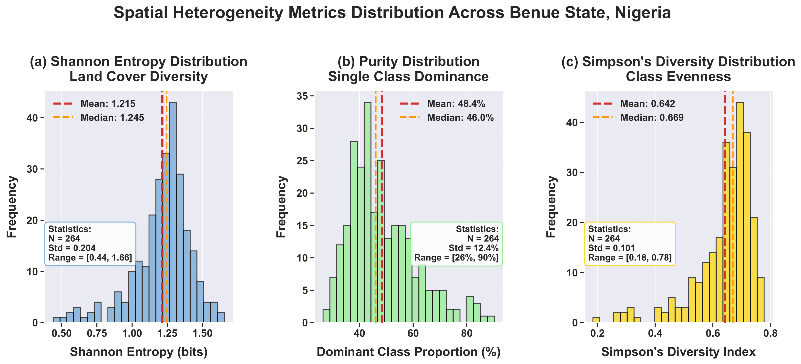
Spatial representativeness was quantified using ESA WorldCover-derived heterogeneity metrics within each 0.1° grid cell. Across 264 grid cells, the mean dominant-class proportion was 48.4%, the median was 46.0%, and the mean Shannon entropy was 1.215. Cropland was the dominant class in 123 locations (46.6%), tree cover in 77 locations (29.2%), shrubland in 34 locations (12.9%), and grassland in 30 locations (11.4%). These values confirm that Benue State is a mixed agricultural–woodland mosaic rather than a spatially uniform surface.

The distribution of the sub-grid heterogeneity metrics is shown in Figure 10. The concentration of Shannon entropy around 1.2, mean dominant-class proportion below 50%, and high Simpson diversity values confirm that many analysis cells contain mixed land-cover compositions rather than single homogeneous surfaces.

The relationship between land-cover heterogeneity and location-level CYGNSS ETC correlation was weak. Among the 142 locations with converged location-level ETC estimates, Spearman correlation between Shannon entropy and CYGNSS r was $-0.155$ ($p=0.051$); Simpson’s diversity index had $\rho =-0.127$ ($p=0.110$); and dominant-class proportion had $\rho =0.064$ ($p=0.422$). These diagnostics indicate that sub-grid heterogeneity contributes representativeness uncertainty, but it does not dominate the regional CYGNSS performance pattern.

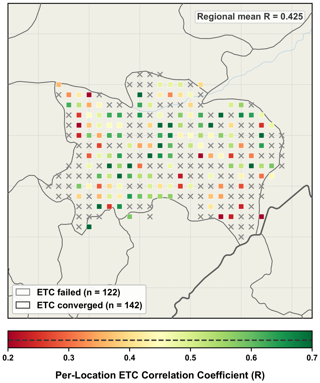
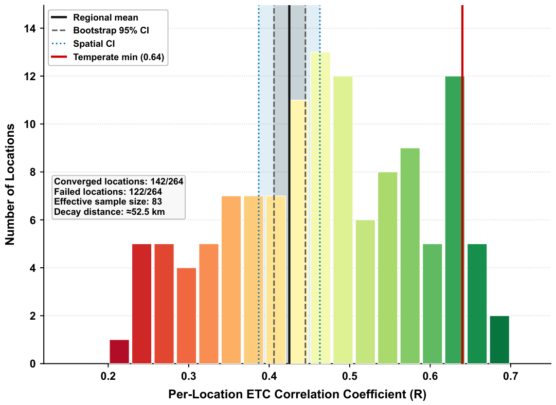
The spatial pattern of location-level CYGNSS ETC performance is shown in Figure 11, and the distribution of converged location-level correlations is summarized in Figure 12. These figures provide spatial context for the weak land-cover heterogeneity relationships reported in

Table 8. Sub-grid land-cover heterogeneity and relationship with location-level CYGNSS ETC performance.

Metric	Mean	Median	Range/Test	Interpretation
Shannon entropy	1.215	1.245	0.439–1.655	High land-cover diversity within many 0.1° cells.
Dominant-class proportion	48.4%	46.0%	—	Many grid cells are mixed rather than pure land-cover units.
Simpson diversity index	0.642	—	0.184–0.778	Confirms moderate-to-high sub-grid diversity.
Entropy vs. CYGNSS r	—	—	$\rho =-0.155,p=0.051$	Weak negative relationship; not significant at 0.05.
Purity vs. CYGNSS r	—	—	$\rho =0.064,p=0.422$	No evidence that purer cells systematically increase CYGNSS r.

Note: An em dash (—) indicates that the corresponding statistic is not reported or is not applicable to that row.

.

Therefore, footprint mismatch and mixed-pixel effects should be acknowledged as sources of representativeness uncertainty, especially in highly heterogeneous cells. However, the available diagnostics do not indicate that they overturn the regional ETC and stratification conclusions.

3.7. Seasonal and Harmattan-Period Performance Failure

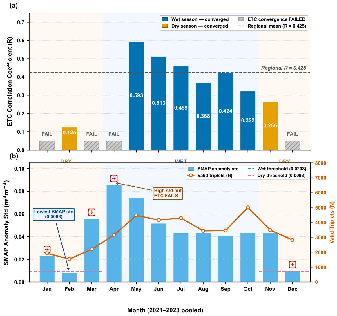
Seasonal diagnostics show that the dry season is the main operational weakness. Wet-season CYGNSS performance improved to $r=0.497$ using 28,015 triplets. Dry-season location-level ETC failed to converge, despite 11,988 dry-season triplets at the pooled level. Additional diagnostics were conducted to determine whether this failure reflected numerical ill-conditioning or a loss of coherent CYGNSS anomaly structure under Harmattan/dry-soil conditions.

The covariance condition number remained moderate in both seasons: 4.79 in the wet season and 7.18 in the dry season. Standard ETC and variance-normalized ETC both converged in the wet season and produced the same CYGNSS estimate $(r=0.4968)$. In the dry season, both standard and variance-normalized ETC failed because of negative error variance estimates. Since variance normalization did not restore convergence and the covariance condition number was not extreme, the failure is unlikely to be explained by numerical scaling alone.

Seasonal variance and covariance diagnostics show the underlying structure of the failure (

Table 9. Seasonal sampling, variance, covariance, and convergence diagnostics. Values use 31-day centered anomalies.

Metric	Wet Season	Dry Season	Dry/Wet or Change
Season definition	April–October	November–March	—
Valid triplets	28,015	11,988	—
CYGNSS coverage	24.2%	13.3%	—
SMAP soil moisture mean	0.2591 ${\mathrm{m}}^3{\mathrm{m}}^{-3}$	0.0956 ${\mathrm{m}}^3{\mathrm{m}}^{-3}$	—
SMAP observations below 0.15 ${\mathrm{m}}^3{\mathrm{m}}^{-3}$	12.2%	84.3%	—
CYGNSS anomaly variance	0.001672	0.001371	0.820
SMAP anomaly variance	0.003201	0.001305	0.408
ERA5-Land anomaly variance	0.000781	0.000336	0.430
CYGNSS–SMAP covariance	0.000787	0.000359	0.456
CYGNSS–ERA5-Land covariance	0.000145	0.000075	0.517
SMAP–ERA5-Land covariance	0.000276	0.000311	1.127
CYGNSS–SMAP correlation	0.3403	0.2682	−0.0722
CYGNSS–ERA5-Land correlation	0.1266	0.1101	−0.0165
SMAP–ERA5-Land correlation	0.1746	0.4700	+0.2954
Covariance condition number	4.79	7.18	Moderate in both seasons
ETC result	$r=0.4968$	Failed at location level	Dry-season failure

Note: An em dash (—) indicates that the dry/wet comparison is not applicable for the corresponding row.

). SMAP anomaly variance decreased by 59.2% from wet to dry season, ERA5-Land anomaly variance decreased by 57.0%, and CYGNSS anomaly variance decreased by 18.0%. More importantly, CYGNSS covariance with SMAP decreased by 54.4%, and CYGNSS covariance with ERA5-Land decreased by 48.4%, whereas SMAP–ERA5-Land covariance increased by 12.7%. Pairwise correlations showed the same selective pattern: CYGNSS–SMAP and CYGNSS–ERA5-Land correlations declined during the dry season, while SMAP–ERA5-Land correlation increased from 0.1746 to 0.4700.

These diagnostics indicate that Harmattan-period failure is not simply a mathematical covariance-collapse artifact. It is more consistent with reduced anomaly variance and selective CYGNSS decoupling from the SMAP–ERA5-Land anomaly structure under dry-season conditions. This interpretation remains cautious: the diagnostics do not prove a single physical mechanism, but they support the conclusion that dry-season CYGNSS anomaly coherence is weaker than during the wet season.

Monthly diagnostics show that the core wet-season months produced the most reliable ETC solutions. January, March, April, and December failed to converge, while February and November converged but produced very low correlations. These results show that CYGNSS is weakest during the period when early detection of agricultural drought stress is most important. Figure 13 illustrates the monthly convergence pattern and the Harmattan-period signal reduction.

3.8. Sensitivity and Robustness of the ETC Results

Sensitivity and robustness diagnostics were used to test whether the primary regional ETC result was stable under alternative processing choices, sampling conditions, and uncertainty assumptions. The diagnostics focused on five issues: anomaly-window length, sample-size dependence, bootstrap seed stability, spatial autocorrelation, and cross-validation. Detailed numerical outputs are provided in Appendix A, while the main implications are summarized here.

The anomaly-window test shows that the CYGNSS ETC estimate is sensitive to very short anomaly windows but stabilizes once the window captures broader sub-seasonal variability. The 7-day window produced the weakest result, with $r=0.1840$, estimated error standard deviation $=0.022944{\mathrm{m}}^3{\mathrm{m}}^{-3}$, and SNR $=-14.55$ dB. The 14-day and 21-day windows increased the correlation to $r=0.3182$ and $r=0.3853$, respectively. The selected 31-day centered window gave $r=0.4253$, estimated error standard deviation $=0.036007{\mathrm{m}}^3{\mathrm{m}}^{-3}$, and SNR $=-6.56$ dB. Longer windows produced comparable estimates, with $r=0.4127$, $0.4266$, and $0.4464$ for the 40-, 50-, and 60-day windows, respectively. These results indicate that windows shorter than about three weeks under-represent the sub-seasonal anomaly structure, whereas the 31-day centered window provides a stable estimate without imposing the stronger smoothing associated with the longest windows.

Sample-size sensitivity confirms that the regional estimate is not an artifact of the full pooled sample. Repeated subsampling at 75%, 50%, and 25% of the valid triplets kept CYGNSS r within a narrow interval of 0.419 to 0.432. Even at the 25% sampling level, each replicate retained approximately 9935 valid records, and the resulting estimates remained close to the full-sample value of $r=0.4253$. This demonstrates that the primary ETC result is stable under substantial random reduction of the collocated sample.

Bootstrap seed testing further supports numerical reproducibility. Eleven independent bootstrap seeds were tested using 1000 iterations per seed. Across these runs, CYGNSS r had a mean of 0.4254, a standard deviation of 0.000276, and a total range of only 0.000744. SMAP r varied by only 0.0018 across the same seed set, and no failed bootstrap iterations occurred. The confidence intervals are therefore not materially affected by the random seed used during resampling.

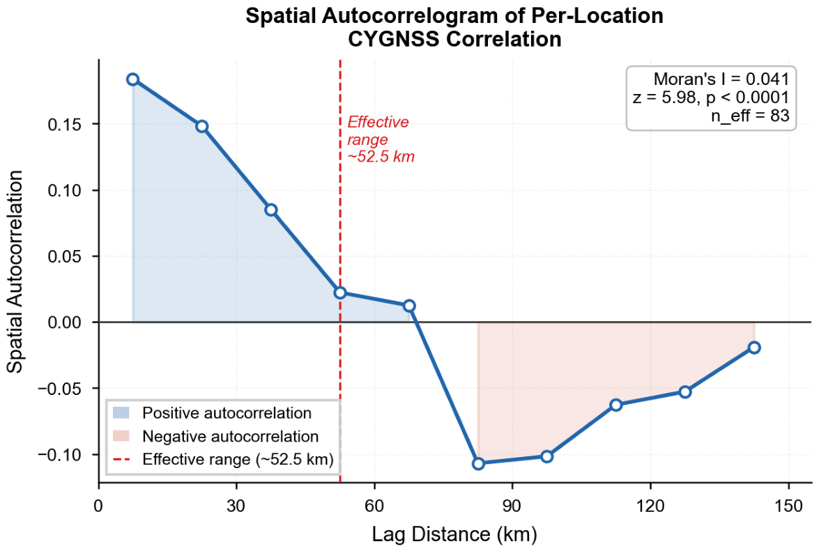
Spatial dependence was present but did not change the interpretation. Location-level ETC converged in 142 of the 264 grid cells. Moran’s $I=0.041$ indicated modest positive spatial autocorrelation, and the Clifford correction reduced the effective sample size to $n_{\mathrm{eff}}=83$. The spatially adjusted 95% confidence interval for CYGNSS r was [0.387, 0.463]. Although this interval is wider than the ordinary bootstrap interval, it remains consistent with the conclusion that CYGNSS has measurable but limited ETC-derived anomaly-tracking skill across the study region.

The distance-decay structure used to support the spatial autocorrelation correction is shown in Figure 14.

Overall, the robustness diagnostics support the reliability of the regional ETC interpretation. The CYGNSS estimate remains stable under subsampling, bootstrap repetition, spatial adjustment, and random cross-validation. The main sources of variation are anomaly-window length and temporal seasonality, both of which are physically meaningful for a strongly seasonal Guinea savanna environment. The primary limitation is therefore not statistical instability of the pooled ETC estimate, but the reduced CYGNSS anomaly coherence under dry-season, Harmattan, dense-vegetation, and tree-cover conditions documented in the environmental and seasonal analyses. The principal robustness diagnostics and their implications are summarized in

Table 10. Robustness diagnostics for the primary CYGNSS ETC result. Full diagnostic outputs are provided in Appendix A.

Diagnostic	Main Result	Implication
Anomaly-window sensitivity	CYGNSS r increased from 0.1840 at 7 days to 0.4253 for the 31-day centered window. Longer 40–60-day windows gave similar values of 0.4127–0.4464.	Very short windows are unstable. The 31-day centered window provides a stable sub-seasonal anomaly definition without excessive smoothing.
Sample-size stability	Repeated 75%, 50%, and 25% subsampling kept CYGNSS r within 0.419–0.432.	The regional ETC estimate is not controlled by the full pooled sample size.
Bootstrap seed stability	Eleven bootstrap seeds gave mean CYGNSS $r=0.4254$, standard deviation $=0.000276$, and range $=0.000744$.	The point estimate and confidence intervals are reproducible across resampling seeds.
Spatial autocorrelation correction	Location-level ETC converged in 142 of 264 grid cells. Moran’s $I=0.041$, $n_{\mathrm{eff}}=83$, and the spatially adjusted 95% CI was [0.387, 0.463].	Spatial dependence widens uncertainty but does not change the interpretation of measurable but limited CYGNSS anomaly-tracking skill.

, while the complete numerical outputs are provided in Appendix A.

These diagnostics clarify the role of the Appendix A. The main manuscript reports the values needed to support the conclusions, while Appendix A provides the complete numerical tables for verification. Overall, the robustness tests show that the primary CYGNSS ETC estimate is stable under resampling, reproducible under bootstrap seed changes, only modestly affected by spatial dependence, and physically consistent with the seasonal and environmental stratification results.

3.9. Cross-Validation Robustness

Three complementary cross-validation approaches were applied to test whether the primary ETC result generalizes beyond the full pooled dataset. The full-dataset CYGNSS correlation was $r=0.4253$ for 40,003 valid triplets.

Table 11. Cross-validation robustness assessment for the primary CYGNSS ETC correlation. The full-dataset reference is $r=0.4253$, with $N=40,003$. Random, spatial, and temporal partitions evaluate generalization across sample composition, geography, and time. An em dash indicates that a fold-based statistic is not applicable to the full pooled dataset.

CV Approach	Folds	Held-Out Fold r Values	Mean r	Std.	Range
Random 10-fold	10	0.3932, 0.4079, 0.4205, 0.4678, 0.4531, 0.4176, 0.3934, 0.4198, 0.4258, 0.4624	0.4261	0.0253	0.0746
Spatial 4-fold	4	NW: 0.4612; NE: 0.4635; SE: 0.4852; SW: 0.5305	0.4851	0.0321	0.0693
Temporal leave-one-year-out	3	2021: 0.4344; 2022: 0.5430; 2023: 0.3606	0.4460	0.0749	0.1824
Temporal 5-fold	5	0.4806, 0.3344, 0.6731, 0.4188, 0.2680	0.4350	0.1393	0.4051
Full dataset reference	—	Full pooled ETC sample	0.4253	—	—

summarizes the random, spatial, and temporal cross-validation results.

Random 10-fold cross-validation partitioned the 40,003 valid triplets into ten approximately equal subsets. ETC was applied independently to each held-out fold. CYGNSS r ranged from 0.3932 to 0.4678, with a mean of 0.4261, standard deviation of 0.0253, and range of 0.0746. The estimated error standard deviation remained stable at $0.0360\pm 0.0007{\mathrm{m}}^3{\mathrm{m}}^{-3}$ across the random folds. The close agreement between the random-fold mean and the full-dataset estimate shows that the primary result is not an artifact of the specific sample composition.

Spatial 4-fold cross-validation divided Benue State into four geographic quadrants. Each quadrant was evaluated as a held-out test set while the remaining three quadrants provided the training pool. Test-fold CYGNSS r ranged from 0.4612 in the north-west quadrant to 0.5305 in the south-west quadrant, with a mean of 0.4851 and standard deviation of 0.0321. This consistency indicates that the primary result is not controlled by a single geographic subregion. The modest positive offset relative to the pooled result reflects the compositional effect of spatial partitioning, because geographically concentrated dry-season observations suppress the aggregate correlation when pooled.

Temporal cross-validation showed wider variability, as expected from the seasonal diagnostics. Leave-one-year-out validation produced r values of 0.4344 for 2021, 0.5430 for 2022, and 0.3606 for 2023. Temporal 5-fold validation produced values from 0.2680 to 0.6731. The higher temporal spread is physically meaningful. Folds dominated by active wet-season months perform better, while folds spanning dry-season or transition periods perform worse. This pattern independently confirms that seasonal soil moisture dynamics are the dominant driver of CYGNSS retrieval variation across Benue State.

Across all three approaches, random and spatial cross-validation confirm the statistical stability and geographic generalizability of the primary result. Temporal variability reflects genuine environmental seasonality and is consistent with the stratified analyses and convergence diagnostics. Together, the cross-validation tests show that the primary ETC result is robust, reproducible, and representative of CYGNSS retrieval behavior in Guinea savanna tropical agriculture.

3.10. Summary of Key Results

CYGNSS Level 3 soil moisture has measurable but limited ETC-derived anomaly-tracking skill in Guinea savanna agriculture. The SMAP-independent triplet gives a conservative estimate near $r=0.386$, while the SMAP-inclusive configuration gives a modestly higher estimate. QC does not detect significant direct CYGNSS–SMAP error correlation. Performance improves under moderate precipitation and open or agricultural land cover, but weakens under dry soils, persistent tree cover, and Harmattan conditions. Robustness, threshold sensitivity, spatial representativeness diagnostics, and cross-validation tests confirm that these conclusions are stable.

4. Discussion

4.1. Benchmarking Against Published CYGNSS and Soil Moisture Validation Studies

The SMAP-independent CYGNSS estimate of $r=0.386$ is the most conservative measure of CYGNSS anomaly-tracking performance in this study. The full regional SMAP-inclusive ETC value of $r=0.425$ is retained for comparison because many previous CYGNSS assessments use SMAP-related references or in situ networks rather than a SMAP-independent collocation configuration. Both estimates are close to the global CYGNSS triple-collocation range reported in broader product assessments [26]. This suggests that the Guinea savanna result reflects a wider limitation of the current CYGNSS Level 3 soil moisture product under some tropical land conditions rather than a purely local anomaly.

Direct comparison with temperate in situ validation studies requires caution. ETC-derived correlation with a latent statistical signal is not the same metric as Pearson correlation against in situ sensors [13,14]. Still, the magnitude of the gap is informative. Temperate CYGNSS validation and retrieval studies have reported higher correlations under some algorithms and validation settings [22,23,25]. Those results often rely on denser in situ networks, different retrieval algorithms, or regions with different vegetation and moisture dynamics. The present study therefore complements earlier GNSS-R work by focusing on a tropical smallholder region where direct ground validation is not available.

SMAP’s performance provides useful context. SMAP remained the strongest product in both the regional ETC analysis and the CYGNSS-free triplet with ERA5-Land and ESA CCI ACTIVE. This is consistent with its established role as a high-quality L-band soil moisture product [18,20]. The contrast between SMAP and CYGNSS does not remove the value of CYGNSS. Rather, it indicates that CYGNSS’s high revisit frequency requires regional correction and uncertainty screening before it can be used reliably for agricultural drought monitoring.

4.2. Why CYGNSS Degrades in Guinea Savanna Agriculture

The degradation is not random. It is linked to physical and environmental controls. Vegetation affects the propagation and scattering of L-band reflected signals. Dense crop or woodland canopies attenuate the soil contribution and increase the influence of vegetation structure [17,38]. This explains the monotonic NDVI pattern and the weaker performance over tree cover.

Dry soils create a different limitation. GNSS-R retrieval depends on dielectric contrast between soil and air [16]. Under very dry conditions, soil moisture variability can become small, and the retrievable signal is reduced. This problem is strongest during Harmattan months, when moisture variability collapses and the collocation system fails at local scales.

Wet conditions can also reduce performance. High rainfall may introduce surface water, ponding, roughness changes, and mixed scattering responses [39]. The high precipitation stratum performed better than the dry stratum but worse than the moderate precipitation stratum. This supports the interpretation that CYGNSS performs best when soil moisture is changing dynamically but not dominated by extreme wetness or extreme dryness.

Mixed pixels further complicate retrieval. Cropland, shrubland, grassland, and tree cover can coexist within a single retrieval footprint. Such heterogeneity weakens the relationship between grid-cell average soil moisture and the scattering conditions sampled by individual CYGNSS specular points.

4.3. Why Estimated Error Standard Deviation Alone Is Misleading

CYGNSS achieved an ETC-derived estimated error standard deviation of $0.036{\mathrm{m}}^3{\mathrm{m}}^{-3}$, close to the commonly cited $0.04{\mathrm{m}}^3{\mathrm{m}}^{-3}$ accuracy target for L-band soil moisture missions [18,20]. This appears encouraging, but it should not be interpreted as a conventional ground-truth error metric. Collocation-derived error standard deviation is estimated relative to a latent statistical signal under the assumptions of the ETC model.

The negative SNR of $-6.56$ dB indicates that, within the ETC framework, the estimated error variance exceeds the estimated signal variance for CYGNSS anomalies. This is a warning about direct anomaly tracking, not evidence that the product is unusable or devoid of soil moisture information. A product can have a moderate estimated error spread while still having limited ability to track sub-seasonal anomalies reliably. Drought early warning requires detection of onset, persistence, and recovery, which depend on coherent anomaly dynamics rather than average error magnitude alone.

ERA5-Land illustrates the same issue in another way. It had the lowest estimated error standard deviation but the weakest latent anomaly correlation. This suggests that it captures background moisture evolution but is less responsive to some daily or event-scale anomaly dynamics. For drought monitoring, correlation, SNR, seasonal convergence, and environmental robustness must therefore be considered alongside estimated error standard deviation.

4.4. Implications of the SMAP-Inclusive Configuration and QC Diagnostics

The QC analysis changes the interpretation of the CYGNSS–SMAP relationship. The covariance-pathway estimator did not detect statistically significant direct CYGNSS–SMAP error correlation in the Benue anomaly dataset. The estimated cross-error correlation was near zero and its confidence interval included zero. Therefore, the earlier concern about SMAP-related dependence should be framed cautiously: direct error coupling was not confirmed by the QC estimator.

Nevertheless, the triplet sensitivity analysis remains important. The CYGNSS estimate was modestly higher in the SMAP-inclusive triplet than in the SMAP-independent triplet. This means that the SMAP-inclusive configuration is less conservative for interpreting CYGNSS performance, even if the difference cannot be attributed to a large detected cross-error covariance. Possible explanations include product scaling, differences in signal representation, sampling effects, and residual structural dependence associated with the SMAP-trained CYGNSS retrieval history.

This has implications beyond this case study. Future validation of trained satellite products should consider whether a validation reference also appears in the training chain. When such overlap exists, standard triplet assumptions may be weakened or difficult to verify. A fourth structurally distinct product, combined with covariance-pathway diagnostics and triplet sensitivity testing, provides a practical way to evaluate the robustness of the inferred performance estimate [14,40,41].

4.5. Operational Implications for Drought Monitoring

The results do not imply that CYGNSS has no value for drought monitoring. Its high revisit frequency remains attractive, especially in the tropics where rainfall events are frequent and localized [15]. The results instead show that uncorrected CYGNSS Level 3 soil moisture should not be used alone for year-round drought monitoring in Guinea savanna agriculture.

Operational use should be most cautious during dry and Harmattan periods. The dry-condition correlation of $r=0.331$ is low, and severe dry cases are under-sampled. The true performance during the most extreme dryness may therefore be worse than the dry-stratum estimate suggests. Early-warning systems that rely directly on uncorrected CYGNSS anomalies could miss or misrepresent drought onset [42].

CYGNSS may be more valuable in multi-sensor systems. Its revisit frequency can complement SMAP’s accuracy, ERA5-Land’s continuity, precipitation observations, and vegetation information. In such systems, CYGNSS should be used with quality weighting, seasonal flags, and environmental bias correction.

4.6. Preliminary Framework for Environment-Aware Bias Correction

The present study is a diagnostic assessment rather than a correction-model paper. Its purpose is to identify where and why uncorrected CYGNSS Level 3 soil moisture performs well or poorly in Guinea savanna agriculture. The results provide the empirical basis for a separate environment-aware correction framework, which is being developed as follow-up work. This distinction is important: implementing, training, and independently validating a corrected CYGNSS product would require a separate modeling experiment and should not be compressed into the present collocation-focused study.

Nevertheless, the diagnostics identify the covariates that such a correction framework should use. A future correction model should include CYGNSS Level 3 soil moisture and retrieval uncertainty as primary inputs, together with vegetation state, dominant land cover, recent precipitation, soil moisture regime, season, and a Harmattan-period indicator. These variables are justified by the results of this study: performance decreases under dry soils, dense vegetation, tree cover, and Harmattan conditions, while moderate recent precipitation gives the strongest CYGNSS anomaly-tracking performance.

The correction should also be regime-aware. Dry, medium, and wet soil states should not be forced to share the same correction relationship, because the medium soil moisture class consistently performs better than the dry and wet classes. Similarly, cropland and shrubland/grassland should be treated differently from persistent tree cover, and moderate-rainfall cases should be separated from very dry or very wet recent rainfall regimes. A practical future workflow would therefore include quality screening, environmental-regime assignment, regime-specific correction, and uncertainty flagging.

This proposed framework is included to respond to the operational implication of the validation results, not to claim that a corrected product has already been produced. The correction model itself will be the subject of a subsequent study after the present first-stage assessment has established the key error regimes and environmental controls.

4.7. Limitations and Future Work

Several limitations should guide interpretation. First, there are no dense in situ soil moisture stations in the study area that can provide direct ground validation. This is the reason ETC and QC were used, but it also means that the study estimates performance relative to a latent statistical anomaly signal rather than direct agreement with field sensors.

Second, ETC and QC rely on assumptions about linearity, stationarity, error orthogonality, and error independence [13,14]. The QC analysis did not detect significant CYGNSS–SMAP direct error correlation, but the covariance pathways differed and residual indirect dependencies cannot be ruled out. ESA CCI ACTIVE is structurally distinct from CYGNSS and SMAP, but it is not perfectly independent of all land-surface controls.

Third, land cover classes are assigned at 0.1° resolution using majority vote, which simplifies a heterogeneous agricultural–woodland mosaic. The heterogeneity analysis suggests that this does not dominate regional results, but it remains a source of representativeness uncertainty.

Fourth, CYGNSS sampling is uneven across season and soil moisture state. The dry stratum is under-sampled relative to wet conditions, and this likely makes the dry-condition performance estimate optimistic.

Fifth, this study evaluated only the CYGNSS Level 3 v3.2 soil moisture product. Other GNSS-R soil moisture products and retrieval algorithms, including those based on different scattering models, machine learning architectures, or alternative calibration strategies, were not assessed. Direct comparison with these alternative products would help determine whether the performance limitations identified here are specific to the SMAP-trained Level 3 product or general to GNSS-R soil moisture retrieval in tropical environments.

Future work should extend the collocation framework to multiple CYGNSS retrieval algorithms and emerging GNSS-R missions. It should also combine field campaigns, low-cost in situ sensors, regionally calibrated retrieval models, alternative GNSS-R retrieval algorithms, and independent validation sites across West African cropland, savanna, Sahelian drylands, and humid forest margins.

5. Conclusions

This study evaluated CYGNSS Level 3 soil moisture performance in Guinea savanna agriculture using Extended Triple Collocation and covariance-pathway Quadruple Collocation. The results show that CYGNSS has measurable but limited ETC-derived anomaly-tracking skill in Benue State, Nigeria.

The regional SMAP-inclusive ETC estimate gives $r=0.425$, an estimated error standard deviation of $0.036{\mathrm{m}}^3{\mathrm{m}}^{-3}$, and SNR of $-6.56$ dB. In the common quadruplet sample, the SMAP-inclusive CYGNSS estimate was $r=0.423$, while the SMAP-independent estimate was lower at $r=0.386$. QC did not detect statistically significant direct CYGNSS–SMAP error correlation $(r_{\epsilon }=0.0007,95\%\mathrm{CI}[-0.0270,0.0283])$. The SMAP-independent estimate is therefore used as the conservative benchmark, not because large error coupling was confirmed, but because it avoids the SMAP-inclusive configuration and gives a more cautious regional estimate.

The main operational weakness is dry-season performance. CYGNSS performs poorly under dry soils $(r=0.331)$, and location-level ETC convergence fails during Harmattan conditions. Variance, covariance, correlation, and condition-number diagnostics show that this failure is not simply numerical ill-conditioning. It is more consistent with reduced anomaly variance and selective CYGNSS decoupling from the SMAP–ERA5-Land anomaly structure under dry-season conditions.

Environmental stratification shows that performance is controlled by vegetation, soil moisture regime, precipitation, and land cover. CYGNSS performs better over cropland and shrubland or grassland than over tree cover, and it performs best under moderate precipitation. Threshold-sensitivity tests confirm that these conclusions are not artifacts of the selected class boundaries. Spatial heterogeneity diagnostics show that mixed pixels contribute representativeness uncertainty, but they do not dominate the regional performance pattern.

Uncorrected CYGNSS Level 3 soil moisture is therefore not sufficient as a standalone year-round drought-monitoring product in Guinea savanna agriculture. Its high revisit frequency remains useful, but operational application should rely on environment-aware, bias-corrected, multi-sensor systems that include vegetation state, soil moisture regime, precipitation history, land cover, uncertainty screening, and seasonal Harmattan indicators.

References

1. Seneviratne, S.I.; Corti, T.; Davin, E.L.; Hirschi, M.; Jaeger, E.B.; Lehner, I.; Orlowsky, B.; Teuling, A.J. Investigating soil moisture–climate interactions in a changing climate: A review. Earth-Sci. Rev. 2010, 99, 125–161. [Google Scholar] [CrossRef] [Scilit]
2. Dorigo, W.; Wagner, W.; Albergel, C.; Albrecht, F.; Balsamo, G.; Brocca, L.; Chung, D.; Ertl, M.; Forkel, M.; Gruber, A.; et al. ESA CCI Soil Moisture for improved Earth system understanding: State-of-the-art and future directions. Remote Sens. Environ. 2017, 203, 185–215. [Google Scholar] [CrossRef] [Scilit]
3. Bolten, J.D.; Crow, W.T.; Zhan, X.; Jackson, T.J.; Reynolds, C.A. Evaluating the utility of remotely sensed soil moisture retrievals for operational agricultural drought monitoring. IEEE J. Sel. Top. Appl. Earth Obs. Remote Sens. 2010, 3, 57–66. [Google Scholar] [CrossRef] [Scilit]
4. Ford, T.W.; Harris, E.; Quiring, S.M. Estimating root zone soil moisture using near-surface observations from SMOS. Hydrol. Earth Syst. Sci. 2014, 18, 139–154. [Google Scholar] [CrossRef] [Scilit]
5. Dorigo, W.A.; Wagner, W.; Hohensinn, R.; Hahn, S.; Paulik, C.; Xaver, A.; Gruber, A.; Drusch, M.; Mecklenburg, S.; van Oevelen, P.; et al. The International Soil Moisture Network: A data hosting facility for global in situ soil moisture measurements. Hydrol. Earth Syst. Sci. 2011, 15, 1675–1698. [Google Scholar] [CrossRef] [Scilit]
6. Yakubu, C.I.; Ayer, J.; Laari, P.B.; Amponsah, T.Y.; Hancock, C.M. A mutual assessment of the uncertainties of digital elevation models using the triple collocation technique. Int. J. Remote Sens. 2019, 40, 5076–5093. [Google Scholar] [CrossRef] [Scilit]
7. Tyubee, B.T. An analysis of food crop yields and climate relations in Benue State, Nigeria. J. Niger. Meteorol. Soc. 2006, 6, 13–22. [Google Scholar]
8. Terdoo, F.; Adekola, O. Assessing the role of climate-smart agriculture in combating climate change, desertification and improving rural livelihood in Northern Nigeria. Afr. J. Agric. Res. 2014, 9, 1180–1191. [Google Scholar] [CrossRef] [Scilit]
9. Okpe, B.E.; Aye, G.C. Adaptation to climate change by farmers in Makurdi, Nigeria. J. Agric. Ecol. Res. Int. 2015, 2, 46–57. [Google Scholar] [CrossRef] [Scilit]
10. Onyeneke, R.U.; Olayide, O.E.; Tasie, O.; Emenekwe, C.C.; Enyikwola, E.; Peter, H.H.; Deborah, M.H. Benue State Climate-Smart Agriculture (CSA) Profile; NAPA Research Paper No. 7; Feed the Future Nigeria Agricultural Policy Activity; Michigan State University: East Lansing, MI, USA, 2023. [Google Scholar]
11. Dorigo, W.; Himmelbauer, I.; Aberer, D.; Schremmer, L.; Petrakovic, I.; Zappa, L.; Preimesberger, W.; Xaver, A.; Annor, F.; Ardö, J.; et al. The International Soil Moisture Network: Serving Earth system science for over a decade. Hydrol. Earth Syst. Sci. 2021, 25, 5749–5804. [Google Scholar] [CrossRef] [Scilit]
12. Stoffelen, A. Toward the true near-surface wind speed: Error modeling and calibration using triple collocation. J. Geophys. Res. Ocean. 1998, 103, 7755–7766. [Google Scholar] [CrossRef] [Scilit]
13. McColl, K.A.; Vogelzang, J.; Konings, A.G.; Entekhabi, D.; Piles, M.; Stoffelen, A. Extended triple collocation: Estimating errors and correlation coefficients with respect to an unknown target. Geophys. Res. Lett. 2014, 41, 6229–6236. [Google Scholar] [CrossRef] [Scilit]
14. Gruber, A.; Su, C.H.; Zwieback, S.; Crow, W.; Dorigo, W.; Wagner, W. Recent advances in soil moisture triple collocation analysis. Int. J. Appl. Earth Obs. Geoinf. 2016, 45, 200–211. [Google Scholar] [CrossRef] [Scilit]
15. Ruf, C.S.; Chew, C.; Lang, T.; Morris, M.G.; Nave, K.; Ridley, A.; Balasubramaniam, R. A new paradigm in Earth environmental monitoring with the CYGNSS small satellite constellation. Sci. Rep. 2018, 8, 8782. [Google Scholar] [CrossRef] [Scilit] [PubMed]
16. Ulaby, F.T.; Moore, R.K.; Fung, A.K. Microwave Remote Sensing: Active and Passive. Volume 3: From Theory to Applications; Artech House: Norwood, MA, USA, 1986. [Google Scholar]
17. Chew, C.; Small, E. Soil moisture sensing using spaceborne GNSS reflections: Comparison of CYGNSS reflectivity to SMAP soil moisture. Geophys. Res. Lett. 2018, 45, 4049–4057. [Google Scholar] [CrossRef] [Scilit]
18. Entekhabi, D.; Njoku, E.G.; O’Neill, P.E.; Kellogg, K.H.; Crow, W.T.; Edelstein, W.N.; Entin, J.K.; Goodman, S.D.; Jackson, T.J.; Johnson, J.; et al. The Soil Moisture Active Passive (SMAP) mission. Proc. IEEE 2010, 98, 704–716. [Google Scholar] [CrossRef] [Scilit]
19. Kerr, Y.H.; Waldteufel, P.; Richaume, P.; Wigneron, J.P.; Ferrazzoli, P.; Mahmoodi, A.; Al Bitar, A.; Cabot, F.; Gruhier, C.; Juglea, S.E.; et al. The SMOS soil moisture retrieval algorithm. IEEE Trans. Geosci. Remote Sens. 2012, 50, 1384–1403. [Google Scholar] [CrossRef] [Scilit]
20. Colliander, A.; Jackson, T.J.; Bindlish, R.; Chan, S.; Das, N.; Kim, S.B.; Cosh, M.H.; Dunbar, R.S.; Dang, L.; Pashaian, L.; et al. Validation of SMAP surface soil moisture products with core validation sites. Remote Sens. Environ. 2017, 191, 215–231. [Google Scholar] [CrossRef] [Scilit]
21. Chew, C.; Small, E. Description of the UCAR/CU soil moisture product. Remote Sens. 2020, 12, 1558. [Google Scholar] [CrossRef] [Scilit]
22. Eroglu, O.; Kurum, M.; Boyd, D.; Gurbuz, A.C. High spatio-temporal resolution CYGNSS soil moisture estimates using artificial neural networks. Remote Sens. 2019, 11, 2272. [Google Scholar] [CrossRef] [Scilit]
23. Al-Khaldi, M.M.; Johnson, J.T.; O’Brien, A.J.; Balenzano, A.; Mattia, F. Time-series retrieval of soil moisture using CYGNSS. IEEE Trans. Geosci. Remote Sens. 2019, 57, 4322–4331. [Google Scholar] [CrossRef] [Scilit]
24. Clarizia, M.P.; Pierdicca, N.; Costantini, F.; Floury, N. Analysis of CYGNSS data for soil moisture retrieval. IEEE J. Sel. Top. Appl. Earth Obs. Remote Sens. 2019, 12, 2227–2235. [Google Scholar] [CrossRef] [Scilit]
25. Senyurek, V.; Lei, F.; Boyd, D.; Kurum, M.; Gurbuz, A.C.; Moorhead, R. Machine learning-based CYGNSS soil moisture estimates over ISMN sites in CONUS. Remote Sens. 2020, 12, 1168. [Google Scholar] [CrossRef] [Scilit]
26. Deng, X.; Zhu, L.; Wang, H.; Zhang, X.; Tong, C.; Li, S.; Wang, K. Triple collocation analysis and in situ validation of the CYGNSS soil moisture product. IEEE J. Sel. Top. Appl. Earth Obs. Remote Sens. 2023, 16, 1883–1899. [Google Scholar] [CrossRef] [Scilit]
27. Lei, F.; Senyurek, V.; Kurum, M.; Gurbuz, A.C.; Boyd, D.; Moorhead, R.; Crow, W.T.; Eroglu, O. Quasi-global machine learning-based soil moisture estimates at high spatio-temporal scales using CYGNSS and SMAP observations. Remote Sens. Environ. 2022, 276, 113041. [Google Scholar] [CrossRef] [Scilit]
28. Udo, R.K. Geographical Regions of Nigeria; University of California Press: Berkeley, CA, USA, 1970. [Google Scholar]
29. Peel, M.C.; Finlayson, B.L.; McMahon, T.A. Updated world map of the Köppen-Geiger climate classification. Hydrol. Earth Syst. Sci. 2007, 11, 1633–1644. [Google Scholar] [CrossRef] [Scilit]
30. Oguntunde, P.G.; Friesen, J.; van de Giesen, N.; Savenije, H.H.G. Hydroclimatology of the Volta River Basin in West Africa: Trends and variability from 1901 to 2002. Phys. Chem. Earth 2006, 31, 1180–1188. [Google Scholar] [CrossRef] [Scilit]
31. NiMet. 2023 Seasonal Climate Prediction (SCP); Nigerian Meteorological Agency: Abuja, Nigeria, 2023. Available online: http://ngfrepository.org.ng:8080/jspui/handle/123456789/5461 (accessed on 15 January 2026).
32. Chan, S.K.; Bindlish, R.; O’Neill, P.; Jackson, T.; Njoku, E.; Dunbar, S.; Chaubell, J.; Piepmeier, J.; Yueh, S.; Entekhabi, D.; et al. Development and assessment of the SMAP enhanced passive soil moisture product. Remote Sens. Environ. 2018, 204, 931–941. [Google Scholar] [CrossRef] [Scilit] [PubMed]
33. Muñoz-Sabater, J.; Dutra, E.; Agustí-Panareda, A.; Albergel, C.; Arduini, G.; Balsamo, G.; Boussetta, S.; Choulga, M.; Harrigan, S.; Hersbach, H.; et al. ERA5-Land: A state-of-the-art global reanalysis dataset for land applications. Earth Syst. Sci. Data 2021, 13, 4349–4383. [Google Scholar] [CrossRef] [Scilit]
34. Didan, K. MODIS/Terra Vegetation Indices 16-Day L3 Global 250 m SIN Grid V061 [Data Set]; NASA EOSDIS Land Processes Distributed Active Archive Center: Sioux Falls, SD, USA, 2021. [CrossRef]
35. Dorigo, W.; Gruber, A.; De Jeu, R.; Wagner, W.; Stacke, T.; Loew, A.; Albergel, C.; Brocca, L.; Chung, D.; Parinussa, R.; et al. Evaluation of the ESA CCI soil moisture product using ground-based observations. Remote Sens. Environ. 2015, 162, 380–395. [Google Scholar] [CrossRef] [Scilit]
36. Zanaga, D.; Van De Kerchove, R.; Daems, D.; De Keersmaecker, W.; Brockmann, C.; Kirches, G.; Wevers, J.; Cartus, O.; Santoro, M.; Fritz, S.; et al. ESA WorldCover 10 m 2021 v200 [Data Set]; Zenodo: Geneva, Switzerland, 2022. [Google Scholar] [CrossRef]
37. Clifford, P.; Richardson, S.; Hémon, D. Assessing the significance of the correlation between two spatial processes. Biometrics 1989, 45, 123–134. [Google Scholar] [CrossRef] [Scilit]
38. Camps, A.; Park, H.; Pablos, M.; Foti, G.; Gommenginger, C.P.; Liu, P.W.; Judge, J. Sensitivity of GNSS-R spaceborne observations to soil moisture and vegetation. IEEE J. Sel. Top. Appl. Earth Obs. Remote Sens. 2016, 9, 4730–4742. [Google Scholar] [CrossRef] [Scilit]
39. Panciera, R.; Walker, J.P.; Kalma, J.D.; Kim, E.J.; Hacker, J.M.; Merlin, O.; Berger, M.; Skou, N. The NAFE’05/CoSMOS data set: Toward SMOS soil moisture retrieval, downscaling, and assimilation. IEEE Trans. Geosci. Remote Sens. 2008, 46, 736–745. [Google Scholar] [CrossRef] [Scilit]
40. Zwieback, S.; Scipal, K.; Dorigo, W.; Wagner, W. Structural and statistical properties of the collocation technique for error characterisation. Nonlinear Process. Geophys. 2012, 19, 69–80. [Google Scholar] [CrossRef] [Scilit]
41. Pierdicca, N.; Fascetti, F.; Pulvirenti, L.; Crapolicchio, R.; Muñoz-Sabater, J. Quadruple collocation analysis for soil moisture product assessment. IEEE Geosci. Remote Sens. Lett. 2015, 12, 1595–1599. [Google Scholar] [CrossRef] [Scilit]
42. Odunze, A.C.; Kudi, M.T.; Daudu, C.; Adeosun, J.; Ayoola, G.; Amapu, I.Y.; Abu, S.T.; Mando, A.; Ezui, G.; Constance, D. Soil moisture stress mitigation for sustainable upland rice production in the Northern Guinea Savanna of Nigeria. Adv. J. Microbiol. Res. 2015. Available online: https://www.internationalscholarsjournals.com/articles/soil-moisture-stress-mitigation-for-sustainable-upland-rice-production-in-the-northern-guinea-savanna-of-nigeria.pdf (accessed on 9 July 2026).
Figure 1. Study area of Benue State, Nigeria, showing the geographic context for the Cyclone Global Navigation Satellite System (CYGNSS) soil moisture assessment.
Remotesensing 18 03267 g001
Figure 2. Spatial distribution of the observation locations used for the primary collocation analysis across the common 0.1° grid in Benue State. Blue squares indicate grid cells with Soil Moisture Active Passive (SMAP) observations, green circles represent European Centre for Medium-Range Weather Forecasts fifth-generation land reanalysis (ERA5-Land) grid points, and red triangles denote Cyclone Global Navigation Satellite System (CYGNSS) observation locations. Coincident or overlapping symbols indicate locations where two or more products share common spatial coverage, which forms the spatial basis for the harmonized collocation analysis.
Remotesensing 18 03267 g002
Figure 3. Overall processing workflow used for data harmonization, anomaly calculation, collocation analysis, stratification, and robustness diagnostics.
Remotesensing 18 03267 g003
Figure 4. Temporal data coverage for SMAP, CYGNSS, and valid ETC triplets over Benue State from 2021 to 2023. The figure shows sparse CYGNSS sampling and the lower proportion of valid CYGNSS–SMAP triplets relative to SMAP coverage.
Remotesensing 18 03267 g004
Figure 5. Environmental sampling pattern of valid CYGNSS observations over Benue State. Coverage rates are shown across NDVI, soil moisture, and seasonal strata relative to the regional mean of 19.7%.
Remotesensing 18 03267 g005
Figure 6. Monthly CYGNSS valid-observation coverage over Benue State from 2021 to 2023. Coverage is lower during the dry/Harmattan season, especially from November to March.
Remotesensing 18 03267 g006
Figure 7. Regional ETC-derived performance metrics for CYGNSS, SMAP, and ERA5-Land over Benue State from 2021 to 2023 for the primary CYGNSS–SMAP–ERA5-Land configuration. (a) Correlation with the latent soil moisture anomaly signal; (b) ETC-derived estimated error standard deviation in m 3 m − 3 ; and (c) signal-to-noise ratio in decibels. The reference lines indicate the comparison thresholds shown in each panel.
Remotesensing 18 03267 g007
Figure 8. Pairwise kernel-density scatter plots of 31-day centered soil moisture anomalies from 40,003 valid ETC triplets over Benue State from 2021 to 2023. Colour intensity represents local point density, the dashed white line indicates the 1:1 reference, and the yellow line shows the ordinary least-squares regression fit. Panels compare (a) CYGNSS and SMAP, (b) CYGNSS and ERA5-Land, and (c) SMAP and ERA5-Land. The annotations report the sample size, Pearson correlation, root-mean-square error, and bias for each product pair.
Remotesensing 18 03267 g008
Figure 9. CYGNSS ETC-derived correlation stratified by vegetation density, soil moisture regime, seven-day precipitation, and land cover. Bars show point estimates with 95% bootstrap confidence intervals; the dashed line marks the regional mean ( r = 0.425 ), and asterisks indicate significant pairwise differences. Skill is highest under moderate precipitation and open agricultural surfaces, but weakest under dry soils and persistent tree cover.
Remotesensing 18 03267 g009
Figure 10. Distribution of sub-grid land-cover heterogeneity metrics across Benue State. The panels show Shannon entropy, dominant-class proportion, and Simpson’s diversity index within the 0.1° analysis grid cells; dashed red lines indicate regional means.
Remotesensing 18 03267 g010
Figure 11. Spatial distribution of location-level CYGNSS ETC-derived correlations across the Benue State analysis grid. Coloured grid locations indicate the 142 cells where the location-level ETC analysis converged, with colour representing the estimated correlation with the latent soil moisture anomaly signal. Black “X” symbols indicate the 122 grid cells where ETC failed to converge and no valid location-level correlation estimate was obtained.
Remotesensing 18 03267 g011
Figure 12. Distribution of location-level CYGNSS ETC-derived correlations across the 142 grid cells where the analysis converged. The histogram summarizes spatial variability in CYGNSS anomaly-tracking skill across the Benue State analysis grid. The vertical reference lines indicate the regional mean, ordinary bootstrap 95% confidence interval, spatially adjusted confidence interval, and temperate-region reference threshold.
Remotesensing 18 03267 g012
Figure 13. Monthly ETC convergence and signal variability over Benue State from 2021 to 2023. Panel (a) shows monthly CYGNSS ETC-derived correlations, with hatched bars and “FAIL” labels marking months where ETC did not converge; the dashed horizontal line shows the regional mean. Panel (b) shows monthly SMAP anomaly standard deviation and valid triplet counts. The dashed green and pink horizontal lines indicate the wet- and dry-season anomaly-standard-deviation thresholds, respectively. ETC performance is most reliable from May to October, whereas Harmattan and transition months show convergence failure or weak retrieval skill.
Remotesensing 18 03267 g013
Figure 14. Spatial autocorrelogram of location-level CYGNSS ETC-derived correlations across 142 converged grid cells. Positive short-distance autocorrelation declines toward zero at an effective range of about 52.5 km, supporting the spatially adjusted confidence interval.
Remotesensing 18 03267 g014