Triple-Level Topology Awareness Using Hypergraph for Marine Ship Surveillance from SAR Imagery

Highlights

What are the main findings?

• The proposed TLTA framework enables multi-level high-order topology modeling for SAR ship surveillance by integrating input-level, feature-level, and proposal-level hypergraph learning.
• Experimental results on multiple SAR ship datasets demonstrate that TLTA achieves competitive detection performance compared with representative CNN- and Transformer-based methods.

What are the implications of the main findings?

• Hypergraph-based topology modeling provides an approach for capturing complex non-pairwise dependencies in SAR imagery, complementing conventional feature extraction strategies.
• The proposed topology-aware framework enhances the robustness and adaptability of intelligent maritime surveillance under complex inshore and offshore SAR imaging conditions.

Abstract

Marine ship surveillance from synthetic aperture radar (SAR) imagery is extensively studied. Still, previous methods may not fully capture high-order topological relationships, which can limit performance in complex scenarios. To this end, we propose a triple-level topology awareness (TLTA) framework using hypergraphs for effective SAR marine ship surveillance. TLTA dynamically captures higher-order dependencies in latent spaces by hypergraph convolution, addressing a limitation of prior techniques that rely solely on pairwise correlation analysis. TLTA is implemented at three levels—input-level, feature-level, and proposal-level—to obtain gradually enhanced feature representations, known as i-LTA, f-LTA, and p-LTA. i-LTA designs a super-pixel segmentation module (SPSM) to yield compact and semantically similar regions through an efficient iterative clustering, and the resulting regions are used for super-pixel hypergraph construction (SP-HGC) to produce features rich in spatial topology relationships at the input level, and finally, a cross-attention collaborative network (CACN) is constructed to aggregate high-order and low-order features to achieve a synergistic integration of topological structures and key details. f-LTA explores topology awareness in the backbone feature extraction, mainly through feature-adaptive hypergraph construction (FA-HGC), vertex-level feature self-attention (VL-FSA), and edge-level feature self-attention (EL-FSA), to enable comprehensive modeling of complex inter-patch dependencies beyond simplistic pairwise interactions. p-LTA leverages a proposal prediction network (PPN) to yield positive/negative proposals for proposal-guided hypergraph construction (PG-HGC), and then leverages instance-level spatial priors to ensure the topology interactions between feature subsets. Experimental results reveal the competitive performance of TLTA, achieving AP values of 77.9% and 76.4% on SSDD and HRSID, respectively, and demonstrate the efficacy of each strategy.

1. Introduction

Marine ship surveillance is of great value to transportation, trade activities, and fishery monitoring [1,2]. Given the variability of marine environments, synthetic aperture radar (SAR) [3] is more suitable for ship surveillance than optical/infrared sensors [4,5,6,7], as it can operate around the clock and in all weather conditions without being affected by clouds. In addition, spatial resolution is an important factor for SAR target detection, and spotlight or sliding spotlight imaging modes can provide high-resolution SAR imagery for fine target observation [8].

Early scholars mostly used theoretical modeling to search for ships in SAR images. A classical algorithm is the constant false alarm rate (CFAR) [9] that determines the threshold through modeling sea clutter. However, its multi-scenario generalization ability is relatively weak due to inaccurate modeling [10,11]. Recently, deep learning [12] has driven the rapid development of data-driven object detection. Representative models, such as Faster R-CNN [13], YOLO [14,15,16], SSD [17], FPN [18], CenterNet [19], DiffusionDet [20], Sparse R-CNN [21], and DETR [22,23,24,25,26,27], have emerged and have been applied in many interdisciplinary fields. With the increasing release of public datasets in the SAR field, such as SSDD [28], HRSID [29], SAR-Ship-Dataset [30], and SARDet-100K [31], deep learning-based ship surveillance methods have been rapidly promoted and advanced [32,33,34,35,36,37,38,39]. Scholars have designed various improvement strategies [40,41,42,43,44,45,46,47,48,49,50,51,52,53,54] from different perspectives to boost surveillance performance, promoting the progress of SAR intelligent interpretation.

However, previous methods mostly focus on building models and extracting features around CNNs or Transformers, which do not explicitly model high-order topological intrinsic relationships, potentially limiting the expressive power of models in complex scenes. Related studies [55,56,57] demonstrated that CNNs and Transformers have shortcomings in representing high-order semantics, as they cannot differentially model the connection relationships between local and global. This issue remains relatively underexplored in this field, which hinders further improvement of surveillance performance. To address this, we propose a triple-level topology awareness (TLTA) framework based on hypergraphs for robust SAR marine ship surveillance. Through hypergraph computation, TLTA is able to effectively model complex higher-order relationships in latent spaces, effectively addressing the inherent limitations of conventional approaches that are restricted to pairwise correlation analysis. Specifically, TLTA operates through a cascaded architecture comprising input-level (i-LTA), feature-level (f-LTA), and proposal-level (p-LTA) processing stages, each progressively refining feature representations through specialized topology-aware mechanisms. i-LTA initiates the processing pipeline through a super-pixel segmentation module (SPSM), which partitions input data into semantically meaningful clusters through iterative refinement. These segmented regions serve as the foundation for constructing spatial topology representations during super-pixel hypergraph construction (SP-HGC), which explicitly encodes region relationships. The extracted features are subsequently boosted by a cross-attention collaborative network (CACN) that harmonizes high-order topological patterns with original low-order spatial details. At the feature-level, f-LTA combines feature-adaptive hypergraph construction (FA-HGC) with dual self-attention mechanisms—vertex-level feature self-attention (VL-FSA) and edge-level feature self-attention (EL-FSA)—to capture local patch interactions and model global dependencies. The final p-LTA stage leverages a proposal prediction network (PPN) to yield positive/negative region proposal candidates, which serve as input for proposal-guided hypergraph construction (PG-HGC). This process incorporates instance-level spatial priors to explicitly enforce consistent topology modeling between distinct feature subsets, ensuring robust spatial relationship preservation throughout the detection pipeline. Empirical evaluation demonstrates competitive performance on S SSDD [28] and HRSID [29], with AP values of 77.9% and 76.4%, respectively. The systematic analysis of individual components substantiates the critical role of each strategy in driving such performance gain. Validation on larger-scale datasets—SAR-Ship-Dataset [30] and SARDet-100K [31]—reveals TLTA’s robust adaptability to varying data characteristics. Cross-domain experiments in optical and infrared modalities verify its scalable architecture, highlighting potential for broader application scenarios.

The main contributions of our work are summarized below.

• We propose a triple-level topology awareness (TLTA) framework for SAR marine ship surveillance, which progressively models high-order relationships at the input, feature, and proposal levels. By integrating topology awareness throughout these three stages, TLTA enables hierarchical representation of complex non-pairwise dependencies across the detection pipeline.
• We develop dedicated topology-aware mechanisms for the three levels of TLTA. At the input level, i-LTA combines SPSM, SP-HGC, and CACN to model region-level spatial relationships while preserving local details. At the feature level, f-LTA employs FA-HGC together with VL-FSA and EL-FSA to capture high-order dependencies among feature representations. At the proposal level, p-LTA utilizes PPN, PG-HGC, and CDN-FD to model relationships among positive and negative proposals and enhance subsequent feature decoding.
• Extensive experiments on multiple SAR ship datasets validate the effectiveness of the proposed TLTA framework and its constituent components. The results demonstrate consistent improvements over the baseline and competitive performance compared with representative existing methods, together with favorable performance in complex inshore and offshore scenes and large-scale SAR imagery.

2. Related Work

2.1. Object Detection

The landscape of object detection in computer vision has progressed through several phases. The foundation was laid by Faster R-CNN [13], introducing region proposal networks for two-stage detection. This inspired subsequent refinements like Sparse R-CNN [21] with its learnable proposal mechanism. Parallel developments in single-shot detectors produced SSD [17] for efficient multiscale detection and YOLO [15,16] for the optimized speed-accuracy balance. Feature pyramid network [18] revolutionized multiscale feature handling, while CenterNet [19] pioneered keypoint-based approaches. The transformer revolution began with DETR [22], followed by efficiency-focused variants: Conditional DETR [23] accelerated training, DN-DETR [25] introduced query denoising, and DINO [26] improved anchor boxes. Recent innovations include DiffusionDet [20] applying diffusion models, Hyper-YOLO [14] incorporating hypergraph theory, and real-time optimized models [58]. Emerging works like MS-DETR [59] for mixed supervision and DQ-DETR [60] for tiny object detection continue advancing the field, supported by novel backbones like LSNet [61] and EViT [62].

2.2. SAR Marine Ship Surveillance

The field of SAR ship surveillance/detection has seen significant progress through deep learning approaches. Cui et al. [33] proposed dense attention pyramid networks that effectively handle multi-scale ship detection through hierarchical feature fusion. This work was extended by Zhao et al. [34] with their attention receptive pyramid network, which improves small ship detection through receptive field adaptation. The importance of attention mechanisms is further demonstrated by Zhu et al. [35] who developed a multiscale method combining information compensation with feature enhancement. Recent works also show a clear trend toward anchor-free detection. Bai et al. [36] introduced a global context-guided feature balance pyramid, while Fu et al. [40] presented a feature balancing and refinement network, both achieving superior performance without anchor boxes. This shift is particularly evident in Liu et al. [37]’s CLFR-Det, which specifically addresses tiny-ship detection through cross-level feature refinement. Lightweight architectures have gained attention, with Shen et al. [43] developing ELLK-Net for efficient detection using large kernels, and Zhou et al. [45] proposing HRLE-SARDet that maintains accuracy while reducing computational load. Feng et al. [49] further advanced real-time detection with LRTransDet, combining lightweight ViT with multi-scale fusion. The integration of transformers has shown promising results, as seen in Guo et al. [48]’s M2S-DETR, which combines mixed receptive fields with position encoding. Chen et al. [46] broke second-order limitations in transformers through CSnNet’s recursive convolutions, while Yang et al. [47] developed DAFDet with asymptotic fusion enhancement. More novel solutions have emerged for specific challenges: Liu et al. [41] addressed inshore detection through Fourier-based scene transformation. Yue et al. [42] focused on small ships with a generating-anchor network. Hu et al. [44] proposed FINet for simultaneous object-level and pixel-level detection. More recently, Wu et al. [63] proposed SFD-Net to decouple target features from interference and enhance multiscale feature representation for SAR ship detection. These advancements collectively address key challenges in SAR marine ship surveillance while pointing toward future directions in efficient, accurate, and robust detection systems [64,65,66,67]. While they predominantly concentrate on feature extraction and model construction around CNNs or Transformers, their inherent limitations in modeling high-order topological dependencies become evident when confronted with intricate scenarios. This critical gap motivates the adoption of hypergraph-based monitoring paradigms in this work, which are specifically designed to address these structural modeling deficiencies.

3. Materials and Methods

3.1. HyperGraph Learning

For the sake of a clear introduction, we give the notation summary used in this paper for hypergraph description, as shown in

Table 1. Notation summary.

Notation	Meaning	Notation	Meaning
$G=\left\{V,E,W\right\}$	Hypergraph	$H\in {ℝ}^{N\times M}$	Hypergraph incidence matrix
$v$	Vertex	$h\left(v,e\right)$	Entry in the incidence matrix
$N=\left|V\right|$	Number of vertices	$D_v\in {ℝ}^{N\times N}$	Vertex degree matrix
$V=\left\{v_1,v_2,\cdots ,v_N\right\}$	Vertex set	$d\left(v\right)$	Vertex degree
$e$	Hyperedge	$D_e\in {ℝ}^{M\times M}$	Hyperedge degree matrix
$M=\left|E\right|$	Number of hyperedges	$\delta \left(e\right)$	Hyperedge degree
$E=\left\{e_1,e_2,\cdots ,e_M\right\}$	Hyperedge set	$d$	Vertex feature dimension
$W\in {ℝ}^{M\times M}$	Hyperedge weight diagonal matrix	$x\in {ℝ}^d$	Vertex feature
$w\left(e\right)$	Hyperedge weight	$X=\left\{x_1,x_2,\cdots ,x_n\right\}$	Vertex feature set.

. A hypergraph is a generalized form of graph theory. Unlike conventional graphs, hyperedges can connect any number of vertices [68,69]. This feature enables it to model high-order multivariate relationships. A hypergraph $G=\left\{V,E,W\right\}$ is formally characterized by its vertex set $V=\left\{v_1,v_2,\cdots ,v_N\right\}$, hyperedge set $E=\left\{e_1,e_2,\cdots ,e_M\right\}$, and hyperedge weight diagonal matrix $W\in {ℝ}^{M\times M}$. The weight $w\left(e\right)$ is assigned to each hyperedge $e\in E$, while the vertex-hyperedge incidence structure is encoded by a $N\times M$ correlation matrix $H\in {ℝ}^{N\times M}$. Here, $N=\left|V\right|$ and $M=\left|E\right|$ denote the cardinalities of $V$ and $E$, respectively, with each element $h\left(v,e\right)$ in $H$ defined by a specific binary relation between vertices and hyperedges, i.e.,

$$h\left(v,e\right)=\left\{\begin{array}{c}1, \mathrm{if} v\in e\\ 0, \mathrm{if} v\notin e\end{array}\right.$$

(1)

The vertex degree $d\left(v\right)$ for any $v\in V$ quantifies the number of hyperedges incident to $v$, while the hyperedge degree $\delta \left(e\right)$ for $e\in E$ measures the cardinality of vertices adjacent to $e$. They are defined by

$$d\left(v\right)={\displaystyle \sum _{e\in E}w\left(e\right)\cdot h\left(v,e\right)}; \delta \left(e\right)={\displaystyle \sum _{v\in V}h\left(v,e\right)}$$

(2)

These two fundamental metrics respectively characterize the local connectivity of vertices and hyperedges within the hypergraph structure. In hypergraph analysis, the normalization process of the incidence matrix $H$ is achieved through the diagonal matrices $D_v=\mathrm{diag}\left(d\left(v_1\right),d\left(v_2\right),\cdots ,d\left(v_N\right)\right)$ and $D_e=\mathrm{diag}\left(\delta \left(e_1\right),\delta \left(e_2\right),\cdots ,\delta \left(e_M\right)\right)$, analogous to conventional graph theory. The vertex degree matrix $D_v\in {ℝ}^{N\times N}$ encodes vertex degrees, while the hyperedge degree matrix $D_e\in {ℝ}^{M\times M}$ contains the degrees of hyperedges along its diagonal, collectively ensuring proper scaling of $H$ during spectral computations.

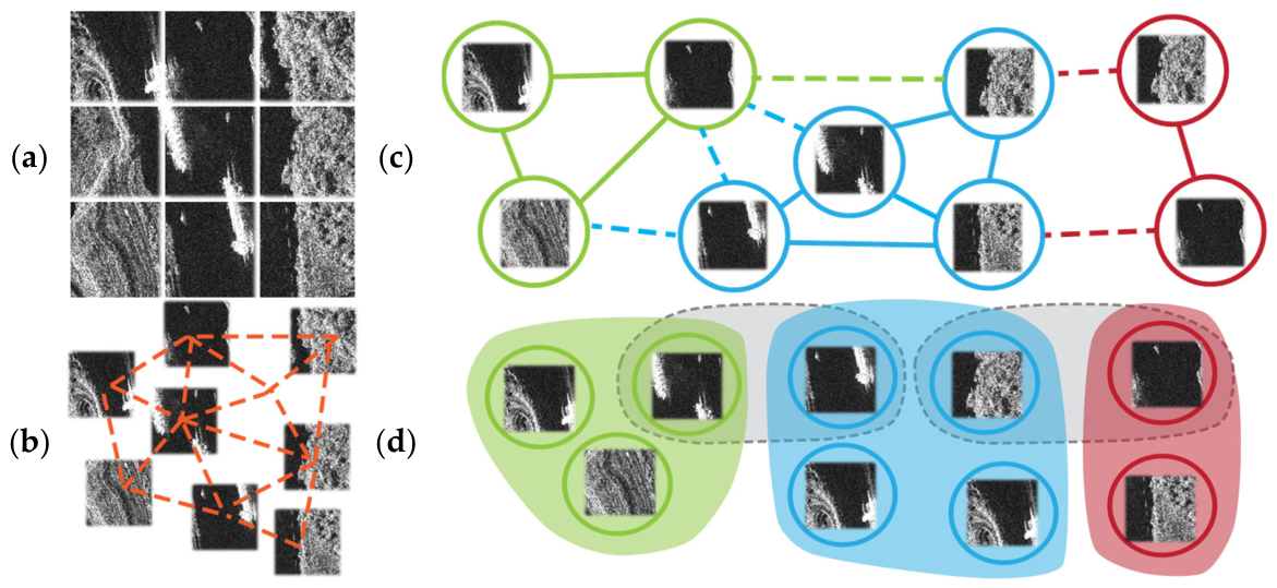
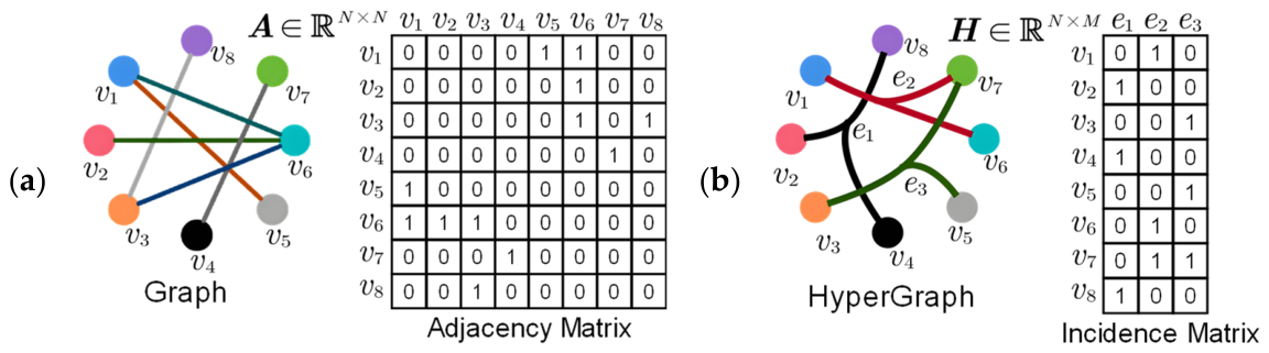
Figure 1 shows the topological correlation structures of different models. The reliance of CNNs on spatially constrained receptive fields introduces inherent limitations in capturing distant feature correlations. This challenge is overcome by Transformers through its patch-wise self-attention mechanism and parallel processing paradigm. Still, Transformer’s effectiveness is contingent upon accurate positional encoding due to its permutation-invariant nature. Traditional graph models further exhibit structural deficiencies, as their edges are restricted to pairwise node connections. Hypergraphs offer a superior alternative through their generalized hyperedge structure, which can simultaneously connect arbitrary vertex subsets, thereby enabling comprehensive modeling of complex higher-order interactions that are inaccessible to conventional graph representations. Figure 2 illustrates the comparison between a graph and a hypergraph. A conventional graph imposes strict structural constraints, as each edge in its adjacency matrix $A\in {ℝ}^{N\times N}$ representation must connect precisely two vertices. This binary limitation fundamentally restricts the modeling capacity to pairwise relationships. In contrast, a hypergraph leverages its incidence matrix $H\in {ℝ}^{N\times M}$ to support hyperedges with variable cardinality, enabling direct representation of complex multi-vertex interactions. This structural flexibility allows hypergraphs to naturally encode high-order intercorrelations that are inaccessible to traditional graph models, particularly when integrating heterogeneous data.

3.2. Proposed HyperGraph Convolution Block

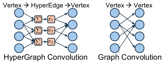
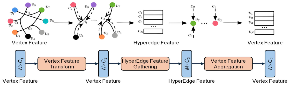
As shown in Figure 3, the graph convolution operates through direct vertex-to-vertex information propagation, leveraging edge connections to facilitate neighborhood aggregation. In contrast, hypergraph convolution introduces a two-stage propagation process where vertex information is first disseminated to hyperedges for intermediate aggregation, followed by redistribution back to vertices. This fundamental difference in propagation pathways stems from their distinct structural representations, with hypergraph convolution requiring hyperedge-mediated information transfer.

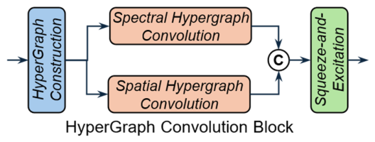
We design a hypergraph convolution block (HGCB) as shown in Figure 4 for feature extraction. From Figure 4, HGCB consists of a hypergraph construction (HGC), a spectral hypergraph convolution, a spatial hypergraph convolution, and a squeeze-and-excitation block (SEB) [70]. A spectral hypergraph convolution ${\psi }_1$ and a spatial hypergraph convolution ${\psi }_2$ implement feature extraction on the constructed hypergraph in parallel, through complementary mechanisms among spectral and spatial domains, whose results are then concatenated for feature aggregation. The motivation for fusing these two branches lies in their different mechanisms for modeling hypergraph topology. The spectral branch captures high-order structural correlations through the first-order Chebyshev approximation of the hypergraph Laplacian, whereas the spatial branch explicitly models vertex–hyperedge–vertex interactions through hyperpath-based message passing. From a representation perspective, the two branches apply different aggregation mechanisms to the same hypergraph: the spectral branch performs Laplacian-based topology filtering, while the spatial branch preserves explicit message propagation along hyperpaths. Therefore, either branch alone captures only one aspect of the hypergraph structure, whereas their parallel fusion preserves both forms of topology information. Finally, SEB is utilized to balance the dual branch channel features, thereby focusing on more valuable information and suppressing redundant ones. The above process can be described as

$$\mathcal{Y}=\mathrm{SEB}\left({\psi }_1\left(\mathrm{HGC}\left(\mathcal{X}\right)\right)\copyright {\psi }_2\left(\mathrm{HGC}\left(\mathcal{X}\right)\right)\right)$$

(3)

3.2.1. Spectral Hypergraph Convolution

For a hypergraph $G=\left\{V,E,W\right\}$ with its Laplacian matrix $W$ being $N\times N$ positive semi-definite, spectral analysis can be performed through eigen decomposition $W=\Phi \Lambda {\Phi }^{\top }$, where $\Phi =\mathrm{diag}\left({\varphi }_1,{\varphi }_2,\cdots ,{\varphi }_N\right)$ contains orthonormal eigenvectors and $\Lambda =\mathrm{diag}\left({\lambda }_1,{\lambda }_2,\cdots ,{\lambda }_N\right)$ is a diagonal matrix of non-negative eigenvalues. These eigenvectors serve as Fourier bases for hypergraph signals, while eigenvalues act as frequency components. The Fourier transform of a signal $X=\left(x_1,x_2,\cdots ,x_N\right)$ is then given by $\widehat{X}={\Phi }^{\top }X$, enabling spectral convolution between a signal $X$ and filter $g$ as

$$g○X=\Phi \left(\left({\Phi }^{\top }g\right)⊚\left({\Phi }^{\top }X\right)\right)=\Phi g\left(\Lambda \right){\Phi }^{\top }X$$

(4)

where $⊚$ denotes the Hadamard product, and $g\left(\Lambda \right)=\mathrm{diag}\left(g\left({\lambda }_1\right),g\left({\lambda }_2\right),\cdots ,g\left({\lambda }_N\right)\right)$ denotes the Fourier coefficient matrix. Given the prohibitive cost of exact Fourier transforms, we employ polynomial parameterization of $g\left(\Lambda \right)$. Specifically, $K$-order polynomials approximate the behavior of $g\left(\Lambda \right)$, enabling efficient computation without explicit spectral decomposition. The Chebyshev polynomials $T_k$, defined by the recurrence $T_k\left(x\right)=2x{T}_{k-1}\left(x\right)-T_{k-2}\left(x\right)$ with $T_0\left(x\right)=1$ and $T_1\left(x\right)=x$, offer a numerically robust basis for approximating $g\left(\Lambda \right)$. Truncate the expansion $g\left(\Lambda \right)$ as,

$$g○X\approx {\displaystyle {\displaystyle \sum _{k=0}^K}{\theta }_k{T}_k\left(\tilde{W}\right)X}$$

(5)

where $T_k\left(\tilde{W}\right)$ corresponds to the $k$-th order Chebyshev basis function, constructed using the scaled Laplacian operator $\tilde{W}=2W/{\lambda }_{\max }-I$. By circumventing the computationally intensive step of Laplacian eigenvector decomposition, it exclusively relies on matrix power operations, additions, and multiplications, thereby achieving significant complexity reduction. This computational advantage is further enhanced by setting $K=1$, as the hypergraph Laplacian inherently captures high-order node interactions without requiring higher-order polynomial expansions. The parameter setting ${\lambda }_{\max }=2$, as advocated in [71,72], derives its validity from the intrinsic scale-adjustment capabilities of neural architectures. This configuration permits a streamlined implementation of the convolution operation without sacrificing representational capacity, i.e.,

$$g○X\approx {\theta }_{0}X-{\theta }_1{D}_v^{-1/2}HW{D}_e^{-1}{H}^{\top }{D}_v^{-1/2}X$$

(6)

To prevent overfitting, the model consolidates the two filter parameters ${\theta }_0$ and ${\theta }_1$ into a unified parameter $\theta$, defined by

$${\theta }_0=-{\displaystyle \frac{1}{2}}\theta ,{\theta }_1={\displaystyle \frac{1}{2}}\theta D_v^{-1/2}H{D}_e^{-1}{H}^{\top }{D}_v^{-1/2}$$

(7)

Then, the convolution operation can be reformulated as

$$\begin{array}{l}g○X\approx \theta D_v^{-1/2}H\left(W+I\right)D_e^{-1}{H}^{\top }{D}_v^{-1/2}X/2\\ \approx \theta D_v^{-1/2}HW{D}_e^{-1}{H}^{\top }{D}_v^{-1/2}X\end{array}$$

(8)

where $W+I$ effectively represents the hyperedge weight matrix. Here, $W$ is initialized as an identity matrix, ensuring uniform weighting across all hyperedges during the initial phase of computation. At each layer $l$, the hypergraph signal $X^l$ undergoes the following transformation by

$$X^{l+1}=\sigma \left(D_v^{-1/2}HW{D}_e^{-1}{H}^{\top }{D}_v^{-1/2}{X}^t\Theta \right)$$

(9)

where $\Theta$ is the adaptive weight matrix. The vertex-wise application of $\Theta$ facilitates localized feature aggregation, yielding $X^{l+1}$ that propagates through the entire network.

As illustrated in Figure 5, spectral hypergraph convolution is implemented through a vertex–hyperedge–vertex transformation framework to effectively capture high-order structural correlations. The process begins with the vertex feature matrix $X^1$ being filtered through the learnable parameter ${\Theta }^1$ to generate $C_2$-dimensional representations. These vertex features are then aggregated by the hyperedge incidence matrix $H$ to form hyperedge-level features ${ℝ}^{M\times C_2}$. Subsequent vertex feature reconstruction is achieved by reapplying the incidence matrix $H$, with normalization factors $D_v$ and $D_e$ ensuring stable feature propagation throughout the iterative refinement process.

3.2.2. Spatial Hypergraph Convolution

Images and simple graphs share a common computational framework where vertices with local connections support spatial aggregation operations. In image processing, each pixel vertex with $C$-dimensional features undergoes neighborhood feature aggregation through mean-pooling after transformation. This spatial convolution paradigm is mirrored in simple graphs, where graph convolution operations collect neighboring vertex features to update central node representations. The message passing mechanism in spatial graph convolution strictly follows the path definition in simple graphs, establishing a consistent information flow from peripheral vertices to the central vertex. In graph theory, a path $P\left(v_1,v_k\right)=\left(v_1\to v_2\to \cdots \to v_k\right)$ is formally defined as an ordered sequence of vertices where consecutive elements maintain adjacency relationships. Specifically, for any vertex pair $\left(i, i+1\right)$ within the sequence, an edge exists connecting them, thereby satisfying the neighbor relation condition throughout the entire path structure.

The spatial hypergraph convolution mechanism derives vertex updates by aggregating neighbor messages along their connecting paths. For each vertex, this involves collecting feature information from adjacent vertices according to the topological paths linking them, thus establishing a systematic method for incorporating hypergraph structure into feature learning. A hyperpath [73] in hypergraph theory is formally defined as an ordered sequence $P\left(v_1,v_k\right)$ connecting distinct vertices $v_1$ and $v_k$, i.e.,

$$P\left(v_1,v_k\right)=\left(v_1\to e_1\to v_2\to e_2\to \cdots \to e_k\to v_k\right)$$

(10)

where each consecutive pair $\left(v_i,v_{i+1}\right)$ must share membership in a common hyperedge, such as $e_i$. This structural constraint ensures that the sequence maintains valid hypergraph connectivity through shared hyperedge participation. Hypergraph message propagation leverages hyperpath connectivity to establish communication channels between vertices through intermediate hyperedges, inherently encoding higher-order structural information compared to standard graph propagation. Introduce inter-neighbor relation $\mathcal{N}$ to extend conventional adjacency concepts to encompass all possible interactions within the combined vertex-hyperedge $V\times E$ space, i.e.,

$$\mathcal{N}=\left\{\left(v,e\right)\left|h\left(v,e\right)=1, v\in V \mathrm{and}\right. e\in E\right\}$$

(11)

The vertex inter-neighbor set ${\mathcal{N}}_v\left(e\right)$ for hyperedge $e$ and the hyperedge inter-neighbor set ${\mathcal{N}}_e\left(v\right)$ for vertex $v$ can be derived from the inter-neighbor relation in (11) as

$${\mathcal{N}}_v\left(e\right)=\left\{v\in V\left|\exists e\in E \mathrm{s}.\mathrm{t}. \left(u\in e\right)\wedge \left(v\in e\right)\wedge \left(u\ne v\right), u\in V\right.\right\}$$

(12)

$${\mathcal{N}}_e\left(v\right)=\{e^{\prime }\in E\left|\right(e\cap e^{\prime }\ne \varnothing )\wedge (e\ne e^{\prime }), e\in E\}$$

(13)

Accordingly, the spatial hypergraph convolution implements hierarchical message passing through hyperpath connectivity. For a given vertex $\alpha \in V$ in the hypergraph $G=\left\{V,E,W\right\}$, first identify its hyperedge inter-neighbor set ${\mathcal{N}}_e\left(\alpha \right)$. To compute messages for each hyperedge $\beta$ within this set, the system further aggregates information from the vertex inter-neighbor set ${\mathcal{N}}_v\left(\beta \right)$, establishing a two-stage propagation mechanism that captures both vertex-hyperedge and hyperedge-vertex interactions. The hypergraph convolution implements a closed message passing loop through two complementary operations, which transform vertex features from $X^l$ to $X^{l+1}$. The $l$-th layer’s spatial hypergraph convolution can be mathematically defined as

$$\begin{array}{cc}\hfill \mathrm{S}\mathrm{t}\mathrm{a}\mathrm{g}\mathrm{e} 1: \{\begin{array}{c}{\displaystyle m_{\beta }^l=\sum _{\alpha \in {\mathcal{N}}_v(\beta )}{M}_v^l(x_{\alpha }^l)}\hfill \\ y_{\beta }^l=U_e^l(w_{\beta },m_{\beta }^l)\hfill \end{array}& \Rightarrow \mathrm{S}\mathrm{t}\mathrm{a}\mathrm{g}\mathrm{e} 2: \{\begin{array}{c}{\displaystyle m_{\alpha }^{l+1}=\sum _{\beta \in {\mathcal{N}}_e(\alpha )}{M}_e^l(y_{\beta }^l)}\hfill \\ x_{\alpha }^{l+1}=U_v^l(w_{\alpha }^l,m_{\alpha }^{l+1})\hfill \end{array}\hfill \end{array}$$

(14)

where the vertex feature transformation updates the input feature vector $x_{\alpha }^l\in X^l$ of vertex $\alpha \in V$ in the layer $l=1,2,\cdots ,L$ to produce the refined feature representation $x_{\alpha }^{l+1}$. The hyperedge message $m_{\beta }^l$ corresponds to the information encoded by the hyperedge $\beta \in E$, with associated weight $w_{\beta }$ quantifying its influence. The vertex message $m_{\alpha }^{l+1}$ represents the transformed feature of the vertex $\alpha$ derived from hyperedge interactions. The hyperedge feature $y_{\beta }^l$ from a hyperedge feature set $Y^l=\left\{y_1^l,y_2^l,\cdots ,y_M^l\left|y_i^l\in {ℝ}^{C_l}\right.\right\}$ in layer $l$ encapsulates the structural characteristics of hyperedge $\beta$ within the current layer’s representation. The $l$-th layer operation is defined by four parametric functions: $M_v^l$ mapping vertex features, $U_e^l$ transforming hyperedge states, $M_e^l$ encoding hyperedge messages, and $U_v^l$ updating vertex representations. These functions constitute a flexible framework whose implementations can be tailored to specific application requirements. By decomposing the convolution process into two distinct stages, the spatial hypergraph convolution effectively models complex hypergraph connectivity. The four learnable operations in this framework handle unordered inter-neighbor relationships through summation aggregation of $M_v^l\left(\cdot \right)$ and $M_e^l\left(\cdot \right)$ messages, combining the permutation-invariant property of traditional graph convolution with enhanced capacity for hypergraph structure representation.

By parameterizing the message-update functions ($M_v^l$, $U_e^l$, $M_e^l$ and $U_v^l$), a fundamental spatial hypergraph convolution operation denoted as

$$\{\begin{array}{c}{M}_v^l\left(x_{\alpha }^l\right)=\frac{x_{\alpha }^l}{|N_v(\beta )|}\hfill \\ U_e^l(w_{\beta },m_{\beta }^l)=w_{\beta }·m_{\beta }^l\hfill \end{array}\Rightarrow \{\begin{array}{c}{M}_e^l(x_{\alpha }^l,y_{\beta }^l)=\frac{y_{\beta }^l}{|N_e(\alpha )|}\hfill \\ U_v^l(x_{\alpha }^l,m_{\alpha }^{l+1})=\sigma \left(m_{\beta }^{l+1}·{\mathit{\Theta }}^l\right)\hfill \end{array}$$

(15)

where the layer-specific parameter ${\Theta }^l\in {ℝ}^{C^l\times C^{l+1}}$ undergoes continuous optimization during training, while $\sigma$ denotes a general non-linear activation function such as ReLU.

The normalized vertex/hyperedge features $x_{\alpha }^l/\left|N_v\left(\beta \right)\right|$ and $y_{\beta }^l/\left|N_e\left(\alpha \right)\right|$ serve dual purposes: facilitating stable convergence through feature standardization and mitigating numerical oscillations during iterative updates. For hardware-accelerated processing, the framework employs matrix operations where $X^l$ represents the vertex features of layer $l$. The hyperedge incidence matrix $H^{\top }\in {\left\{0,1\right\}}^{M\times N}$ orchestrates feature aggregation across the hypergraph structure, producing hyperedge-level representations $Y^l$ through the compact formulation $Y^l=W{D}_e^{-1}{H}^{\top }{X}^l$. The vertex feature update mechanism follows an analogous computational paradigm, where the hyperedge feature set $Y^l$ undergoes a transformation to achieve updated vertex representations $X^{l+1}$ through an operation $X^{l+1}=\sigma \left(D_v^{-1}H{Y}^l{\Theta }^l\right)$. Consequently, the complete spatial hypergraph convolution framework can be mathematically expressed as

$$X^{l+1}=\sigma \left(D_v^{-1}HW{D}_e^{-1}{H}^{\top }{X}^l{\Theta }^l\right)$$

(16)

to encapsulate both feature transformation stages within a unified formulation.

3.3. Overall Framework of Proposed TLTA

For the sake of a clear introduction, we give the abbreviation term used in this paper to describe the proposed TLTA framework, as shown in

Table 2. Abbreviation term summary.

Term	Meaning	Term	Meaning
SPSM	Super-Pixel Segmentation Module	SP-HGC	Super-Pixel HyperGraph Construction
CACN	Cross-Attention Collaborative Network	FA-HGC	Feature-Adaptive HyperGraph Construction
CDN-FD	Contrastive DeNoising Feature Decoding	PG-HGC	Proposal-Guided HyperGraph Construction
DCFE	Dense Contextual Feature Extraction	PP-HGC	Positive Proposal HyperGraph Construction
EL-FSA	Edge-Level Feature Self-Attention	NP-HGC	Negative Proposal HyperGraph Construction
VL-FSA	Vertex-Level Feature Self-Attention	PPN	Proposal Prediction Network
HGCB	HyperGraph Convolution Block	FFN	Feed-Forward Network

.

3.3.1. Overall Framework

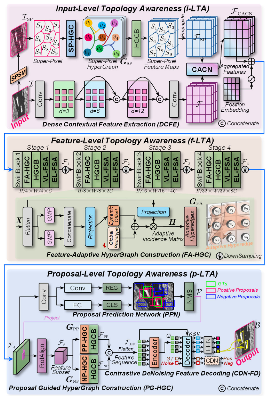
Figure 6 illustrates the overall framework of the proposed TLTA. First, the input SAR image is processed by i-LTA to establish region-level topology relationships and generate enhanced feature representations. Next, f-LTA further models high-order dependencies among intermediate features at different backbone stages to improve feature discriminability. Finally, p-LTA models proposal-level relationships and performs feature encoding and decoding to produce the final ship detection results. The input imagery of TLTA is $\mathcal{I}\in {ℝ}^{H\times W}$. $H$ and $W$ are the height and width. The output is the ship surveillance result $\mathcal{B}={\left\{{\mathcal{B}}_i\right\}}_{i=1}^n$. ${\mathcal{B}}_i=\left(x_i,y_i,w_i,h_i\right)$ is the $i$-th box, $n$ is the number of ships, $\left(x_i,y_i\right)$ is the center, and $w_i$ and $h_i$ are a ship’s width and height.

3.3.2. Execution Process

Algorithm 1 summarizes the execution process of TLTA. First, i-LTA initiates the processing pipeline through its super-pixel segmentation module (SPSM), which yields semantically coherent super-pixel clusters ${\mathcal{I}}_{\mathrm{SP}}=\left\{S_1,S_2,\cdots ,S_n\right\}$ to overcome the limitations of pixel-level fragmentation. This output feeds into the super-pixel hypergraph construction (SP-HGC) component, which constructs a hypergraph $G_{\mathrm{SP}}$, capturing the spatial topology at super-pixel resolution. The previously mentioned hypergraph convolution block (HGCB) is used for feature extraction to enable robust modeling of high-order topological relationships before transforming super-pixel-level features into pixel-aligned representations ${\mathcal{F}}_{\mathrm{SP}}$ through feature propagation. We also incorporate a dense contextual feature extraction (DCFE) to augment the input’s contextual scope, thereby generating enriched scene representations. DCFE yields more comprehensive feature maps $\mathcal{F}$ that encapsulate expanded spatial-semantic relationships beyond the original input dimensions. We notice that direct utilization of super-pixel feature maps leads to undesirable information degradation and detail attenuation, adversely impacting final surveillance results. To address this limitation, a cross-attention collaborative network (CACN) is designed for adaptive feature fusion, which strategically combines high-order structural patterns with low-level discriminative features. CACN enables synergistic enhancement of both global topological relationships and localized salient details through learned attention mechanisms, and its output is denoted by ${\mathcal{F}}_{\mathrm{CACN}}$.

Algorithm 1 Execution Process of TLTA
Input: SAR marine ship surveillance imagery $\mathcal{I}\in {ℝ}^{H\times W}$
Output: TLTA SAR marine ship surveillance result $\mathcal{B}={\left\{{\mathcal{B}}_i\right\}}_{i=1}^n$
Begin
Step 1: Perform Input-Level Topology Awareness (i-LTA)
1:	${\mathcal{I}}_{\mathrm{SP}}\leftarrow \mathrm{SPSM}\left(\mathcal{I}\right)$                                                                                                       //Super-Pixel Segmentation
2:	$G_{\mathrm{SP}}\leftarrow \mathrm{SP}\text{-}\mathrm{HGC}\left({\mathcal{I}}_{\mathrm{SP}}\right)$                                                                                         //HyperGraph for Super-Pixel
3:	${\mathcal{F}}_{\mathrm{SP}}\leftarrow \mathrm{Propagate}\left(\mathrm{HGCB}\left(G_{\mathrm{SP}}\right)\right)$                                                                           //Feature Map of Super-Pixel
4:	$\mathcal{F}\leftarrow \mathrm{DCFF}\left(\mathcal{I}\right)$                                                                                                  //Feature Map of Original Pixel
5:	${\mathcal{F}}_{\mathrm{CACN}}\leftarrow \mathrm{CACN}\left(\mathcal{F},{\mathcal{F}}_{\mathrm{SP}}\right)$                                                                                                         //Feature Fusion
Step 2: Perform Feature-Level Topology Awareness (f-LTA)
6:	$G_{\mathrm{FA}}^{\left(1\right)}\leftarrow \mathrm{FA}\text{-}\mathrm{HGC}\left(\mathrm{SwinBlock}\left({\mathcal{F}}_{\mathrm{CACN}},\mathrm{PE}\right)\right)$                                  //Feature-Adaptive HyperGraph of Stage 1
7:	${\mathcal{F}}_1\leftarrow \mathrm{EL}\text{-}\mathrm{FSA}\left(\mathrm{VLFSA}\left(\mathrm{HGCB}\left(G_{\mathrm{FA}}^{\left(1\right)}\right)\right)\right)\downarrow$                                                         //Feature Extraction of Stage 1
8:	$G_{\mathrm{FA}}^{\left(2\right)}\leftarrow \mathrm{FA}\text{-}\mathrm{HGC}\left(\mathrm{SwinBlock}\left({\mathcal{F}}_1\right)\right)$                                               //Feature-Adaptive HyperGraph of Stage 2
9:	${\mathcal{F}}_2\leftarrow \mathrm{EL}\text{-}\mathrm{FSA}\left(\mathrm{VLFSA}\left(\mathrm{HGCB}\left(G_{\mathrm{FA}}^{\left(2\right)}\right)\right)\right)\downarrow$                                                         //Feature Extraction of Stage 2
10:	$G_{\mathrm{FA}}^{\left(3\right)}\leftarrow \mathrm{FA}\text{-}\mathrm{HGC}\left(\mathrm{SwinBlock}\left({\mathcal{F}}_2\right)\right)$                                              //Feature-Adaptive HyperGraph of Stage 3
11:	${\mathcal{F}}_3\leftarrow \mathrm{EL}\text{-}\mathrm{FSA}\left(\mathrm{VLFSA}\left(\mathrm{HGCB}\left(G_{\mathrm{FA}}^{\left(3\right)}\right)\right)\right)\downarrow$                                                        //Feature Extraction of Stage 3
12:	$G_{\mathrm{FA}}^{\left(4\right)}\leftarrow \mathrm{FA}\text{-}\mathrm{HGC}\left(\mathrm{SwinBlock}\left({\mathcal{F}}_3\right)\right)$                                              //Feature-Adaptive HyperGraph of Stage 4
13	${\mathcal{F}}_4\leftarrow \mathrm{EL}\text{-}\mathrm{FSA}\left(\mathrm{VLFSA}\left(\mathrm{HGCB}\left(G_{\mathrm{FA}}^{\left(4\right)}\right)\right)\right)\downarrow$                                                        //Feature Extraction of Stage 4
Step 3: Perform Proposal-Level Topology Awareness (p-LTA)
14:	$\mathcal{P}\leftarrow \mathrm{PPN}\left({\mathcal{F}}_4\right)$                                                                                                                  //Proposal Prediction
15:	${\mathcal{P}}^{+}\leftarrow \mathrm{IoU}\left(P,P_{\mathrm{GT}}\right)\ge 0.5;$ ${\mathcal{P}}^{-}\leftarrow \mathrm{IoU}\left(P,P_{\mathrm{GT}}\right)<0.5$                                         //Positive or Negative Proposal
16:	${\mathcal{F}}_{\mathrm{S}}\leftarrow \mathrm{RoIAlign}\left({\mathcal{F}}_4,\mathrm{Project}\left(\mathcal{P}\to {\mathcal{F}}_4\right)\right)$                                                                                      //Feature Subset
17:	$G_{\mathrm{PP}}=\mathrm{PP}\text{-}\mathrm{HGC}\left({\mathcal{F}}_{\mathrm{S}}\left|{\mathcal{P}}^{+}\right.\right);$ ${\mathcal{F}}_{\mathrm{PP}}\leftarrow \mathrm{HGCB}\left(G_{\mathrm{PP}}\right)$                                         //HyperGraph for Positive Proposal
18:	$G_{\mathrm{NP}}=\mathrm{NP}\text{-}\mathrm{HGC}\left({\mathcal{F}}_{\mathrm{S}}\left|{\mathcal{P}}^{-}\right.\right);$ ${\mathcal{F}}_{\mathrm{NP}}\leftarrow \mathrm{HGCB}\left(G_{\mathrm{NP}}\right)$                                     //HyperGraph for Negative Proposal
19:	${\mathcal{F}}_{\mathrm{ED}}=\mathrm{Flatten}\left({\mathcal{F}}_{\mathrm{PP}}\copyright {\mathcal{F}}_{\mathrm{NP}}\right)$                                                     //Feature Sequence for Encoding and Decoding
20:	${\mathcal{Q}}_{\mathrm{E}}\leftarrow {\mathcal{F}}_{\mathrm{ED}};$ ${\mathcal{K}}_{\mathrm{E}}\leftarrow {\mathcal{F}}_{\mathrm{ED}};$ ${\mathcal{V}}_{\mathrm{E}}\leftarrow {\mathcal{F}}_{\mathrm{ED}}$                                                                   //Query, Key, Value for Encoder
21:	${\mathcal{F}}_{\mathrm{D}}\leftarrow \mathrm{Encoder}\left({\mathcal{Q}}_{\mathrm{E}},{\mathcal{K}}_{\mathrm{E}},{\mathcal{V}}_{\mathrm{E}},\mathrm{PE}\right)$                                                                                        //Feature Encoding
22:	${\mathcal{Q}}_{\mathrm{D}}\leftarrow {\mathcal{F}}_{\mathrm{D}};$ ${\mathcal{K}}_{\mathrm{D}}\leftarrow {\mathcal{F}}_{\mathrm{ED}};$ ${\mathcal{V}}_{\mathrm{D}}\leftarrow {\mathcal{F}}_{\mathrm{ED}}$                                                                   //Query, Key, Value for Decoder
23:	$\mathcal{B}\leftarrow \mathrm{FFN}\left(\mathrm{Decoder}\left({\mathcal{Q}}_{\mathrm{D}},{\mathcal{K}}_{\mathrm{D}},{\mathcal{V}}_{\mathrm{D}},\mathrm{PE}\right)\left|\mathrm{CDN}\right.\right)$                                                                   //Feature Decoding
End

Then, f-LTA receives ${\mathcal{F}}_{\mathrm{CACN}}$ augmented with position embedding (PE) from the i-LTA output. The Sine encoding scheme functions as spatial prior preservation, defined by

$$\mathrm{PE}\left(pos,2i\right)=\sin \left({\displaystyle \frac{pos}{{10,000}^{2i/d}}}\right); \mathrm{PE}\left(pos,2i+1\right)=\cos \left({\displaystyle \frac{pos}{{10,000}^{2i/d}}}\right)$$

(17)

where $pos\in \left\{x,y\right\}$, $i\in \left\{0,1,\cdots , d/2-1\right\}$ and $d=256$ is the embedding dimension. PE critically maintains locational fidelity during feature transformation to facilitate the operational efficacy of the subsequent SwinBlock [74]. f-LTA adopts a four-stage hierarchical architecture aligned with conventional backbone models, where progressive semantic enrichment and spatial reduction are systematically achieved. The feature map of the $i$-th stage is denoted by ${\mathcal{F}}_i$. Within each processing stage, SwinBlock initially generates intermediate feature representations, which subsequently undergo feature-adaptive hypergraph construction (FA-HGC) to produce stage-specific hypergraph structures $G_{\mathrm{FA}}^{\left(i\right)}$. The architecture then applies HGCB for advanced topological modeling on $G_{\mathrm{FA}}^{\left(i\right)}$, complemented via dual self-attention mechanisms—vertex-level feature self-attention (VL-FSA) and edge-level feature self-attention (EL-FSA)—that employ dynamic feature reweighting to enhance complex high-order relationship modeling capabilities. Upon completion of the fourth processing stage, the resultant feature representation ${\mathcal{F}}_4$ serves as the primary input for p-LTA, thereby bridging the feature extraction and proposal generation by structured data propagation within the computational graph.

Finally, p-LTA completes the final computational pipeline by processing proposal-level hypergraph representations through specialized encoding and decoding operations. It transforms the abstracted topological features into concrete marine ship surveillance outputs, effectively translating high-order relationship modeling into actionable detection results. A proposal prediction network (PPN) operates analogously to the RPN in Faster R-CNN, producing initial region proposals for object detection. These candidate bounding boxes $\mathcal{P}$ are subsequently validated by quantitative intersection over union (IoU) analysis with ground truth (GT) $P_{\mathrm{GT}}$, where a predefined threshold determines their classification as either positive ${\mathcal{P}}^{+}$ or negative ${\mathcal{P}}^{-}$ samples. The IoU between $P$ and $P_{\mathrm{GT}}$ is defined by $\left(P\cap P_{\mathrm{GT}}\right)/\left(P\cup P_{\mathrm{GT}}\right)$. Subsequently, the positive proposals (PP) and negative proposals (NP) are projected onto the feature map to extract their respective feature subsets, which are then used for the proposal-guided hypergraph construction (PG-HGC)—positive proposal hypergraph construction (PP-HGC) $G_{\mathrm{PP}}$ and negative proposal hypergraph construction (NP-HGC) $G_{\mathrm{NP}}$. Likewise, HGCB is adopted to process $G_{\mathrm{PP}}$ and $G_{\mathrm{NP}}$ to achieve their respective outputs ${\mathcal{F}}_{\mathrm{PP}}$ and ${\mathcal{F}}_{\mathrm{NP}}$, which are concatenated and then flattened as a feature sequence ${\mathcal{F}}_{\mathrm{ED}}$ for the subsequent encoding and decoding. ${\mathcal{F}}_{\mathrm{ED}}$ combined with PE is input into the encoder to obtain a decoding query ${\mathcal{Q}}_{\mathrm{D}}$, which is used as the decoding key ${\mathcal{K}}_{\mathrm{D}}$ and value ${\mathcal{V}}_{\mathrm{D}}$ itself. Finally, the contrastive denoising feature decoding (CDN-FD) receives ${\mathcal{Q}}_{\mathrm{D}}$, ${\mathcal{K}}_{\mathrm{D}}$, and ${\mathcal{V}}_{\mathrm{D}}$ to collaborate with a feed-forward network (FFN) through the Hungarian matching algorithm to yield marine ship surveillance results $\mathcal{B}$.

3.4. Input-Level Topology Awareness

3.4.1. Super-Pixel Segmentation Module

SPSM produces semantically meaningful super-pixel groupings that effectively address the inherent fragmentation challenges encountered in traditional pixel-based processing methods. The initialization phase computes an approximate sampling interval $S=\sqrt{K/k}$ derived from the target super-pixel count $k$ and total pixel count $K$, partitioning the image plane into regular grid cells. Cluster centers are strategically positioned by identifying pixels with minimal local gradient magnitude within each grid vicinity, ensuring avoidance of edge artifacts and noise contamination. During iterative optimization, distance metrics are computed between cluster centers and pixels within their $S\times S$ neighborhood regions, with pixel reassignment occurring based on minimum distance criteria. The feature vector of the $i$-th pixel combines CIELAB [75] components $\left(l_i,a_i,b_i\right)$ with spatial coordinates $\left(x_i,y_i\right)$ to achieve joint intensity-space and spatial-domain clustering. Derived through a systematic combination of intensity variance $d_I$ and spatial displacement $d_S$, the composite distance metric $D$ quantifying pixel dissimilarity is defined by $D=\sqrt{\left(d_I/m\right)+{\left(d_S/S\right)}^2}$, where $m$ serves as a critical balancing factor between chromatic affinity and geometric cohesion in super-pixel generation. Higher $m$ values prioritize spatial compactness, yielding super-pixels with increased regularity and reduced perimeter-to-area ratios. Conversely, lower $m$ values emphasize boundary adherence at the expense of shape uniformity, producing super-pixels that more precisely follow contours while showing greater variability in dimensional characteristics. $d_I$ and $d_S$ are defined by

$$d_I=\sqrt{{\left(l_j-l_i\right)}^2+{\left(a_j-a_i\right)}^2+{\left(b_j-b_i\right)}^2}, d_S=\sqrt{{\left(x_j-x_i\right)}^2+{\left(x_j-x_i\right)}^2}$$

(18)

where $i$ represents the current pixel index, and $j$ represents the pixel index within a neighborhood window of size $S\times S$ centered on pixel $i$. The iterative refinement phase involves computing mean values for both intensity and spatial coordinates across all pixels belonging to each super-pixel cluster, generating updated center positions. This centroid recalculation and subsequent pixel reallocation cycle continues iteratively until either the convergence criteria are satisfied or the maximum iterations are reached. A final connectivity enforcement step employs component analysis to eliminate fragmentation by reassigning isolated pixels to neighboring super-pixel regions, ensuring topological coherence across all segmented areas. As a result, the semantically coherent super-pixel clusters ${\mathcal{I}}_{\mathrm{SP}}=\left\{S_1,S_2,\cdots ,S_n\right\}$ are yielded. The detailed execution process of SPSM is summarized in Algorithm 2.

Algorithm 2 Execution Process of SPSM
Input: SAR imagery $\mathcal{I}\in {ℝ}^{H\times W}.$ Number of super-pixels $k$
Output: Label matrix $L$
Begin
1:	Sample pixels with a stride size of $S=\sqrt{K/k}.$
2:	Initialize clustering center $C_k={\left(l_k,a_k,b_k,x_k,y_k\right)}^{\top }.$
3:	Move the clustering center to the minimum gradient position in its $3\times 3$ neighbors
4:	Set clustering label $L\left(i\right)=-1$ and $d\left(i\right)=\infty$ for each pixel
5:	repeat
6:	for each clustering center $C_k$ do
7:	for each pixel $i$ in $\mathrm{SearchRegion}\left(C_k\right)$ do
8:	$D=\mathrm{Distance}\left(C_k,i\right)$
9:	if $D<d\left(i\right)$ then
10:	$d\left(i\right)\leftarrow D;$   $L\left(i\right)\leftarrow k$
11:	end if
12:	end for
13:	end for
14:	Calculate the new clustering center.
15:	Set it as the average vector of all pixels belonging to the cluster.
16:	Calculate the residual $E=\Vert C_k^{\mathrm{current}}-C_k^{\mathrm{previous}}{\Vert }_2.$
17:	Until Convergence $E\le \mathrm{threshold}$ or the maximum iterations are attained.
18:	Perform connectivity enforcement to $L$.
End

Figure 7 shows the results of SPSM. From it, the super-pixel generation demonstrates robust region aggregation capabilities, where semantically consistent areas are consolidated into homogeneous clusters, which will enable efficient hypergraph topology formulation by offering meaningful atomic units for higher-level structural representation.

3.4.2. Super-Pixel HyperGraph Construction

SP-HGC is implemented based on the super-pixel ${\mathcal{I}}_{\mathrm{SP}}$ generated by SPSM to generate the super-pixel-level hypergraph $G_{\mathrm{SP}}$. The hyperedges comprising $G_{\mathrm{SP}}$ represent topological groupings of super-pixels with coherent visual attributes. For comprehensive saliency representation, the scale-variant super-pixel aggregation guided by visual feature affinities can be performed, permitting flexible implementation through various established computational approaches in image segmentation and cluster analysis domains. Non-parametric clustering fundamentally relies on a kernel density estimator,

$${\widehat{f}}_k\left(p\right)={\displaystyle \frac{{\xi }_k}{n{\left|\Sigma \right|}^{1/2}}}{\displaystyle \sum _{i=1}^{n}k\left(d_{\mathrm{M}}^2\left(p,p_i,\Sigma \right)\right)}$$

(19)

where $p_i$ denotes the $i$-th super-pixel in ${\mathcal{I}}_{\mathrm{SP}}$, $k\left(\cdot \right)$ denotes a kernel profile defined by $\exp \left(-x/2\right)$, $\Sigma ={\gamma }^{2}I$ denotes an asymmetric positive definite bandwidth matrix with a scaling coefficient $\gamma$, ${\xi }_k$ denotes a normalization constant, and $d_{\mathrm{M}}$ denotes the Mahalanobis distance defined by $\sqrt{{\left({\mathcal{I}}_{\mathrm{SP}}-S_i\right)}^{\top }{\Sigma }^{-1}\left({\mathcal{I}}_{\mathrm{SP}}-S_i\right)}$. The identification of super-pixel cliques can be formulated as a mode detection problem within the density function ${\widehat{f}}_k\left(p\right)$. This computational challenge translates mathematically to solving the gradient equation $\nabla {\widehat{f}}_k\left(p\right)=0$, addressed through an iterative optimization procedure,

$$p^{t+1}=\frac{{\sum }_{i=1}^n{k}^{\prime }\left(d_{\mathrm{M}}^2\left(p^t,p_i,\Sigma \right)\right)p_i}{{\sum }_{i=1}^n{k}^{\prime }\left(d_{\mathrm{M}}^2\left(p^t,p_i,\Sigma \right)\right)}$$

(20)

where $k^{\prime }\left(\cdot \right)$ is the first-order derivative, and $t$ is the iteration number. An efficient variant of agglomerative mean-shift clustering [76] is implemented, incorporating iterative query set compression as a core acceleration mechanism. In the constructed hypergraph, individual modes establish hyperedges that aggregate super-pixels, demonstrating convergent behavior in the iterative procedure. The scaling matrix $\Sigma$ governs the spatial and spectral properties of the resulting hyperedges, while the adjustable $\gamma$ facilitates flexible multi-resolution hyperedge construction through controlled modifications of the clustering process. It enables the production of hierarchical hyperedge sets $\left\{e_i\right\}$, with individual hyperedge $e_i$ capturing structural relationships at varying scales of observation. As a result, the flexible multi-resolution analysis of the underlying data topology through differentiated hyperedge configurations is achieved.

3.4.3. Dense Contextual Feature Extraction

DCFE operates as a contextual expansion module designed to enhance feature diversity through multi-scale processing. As shown in Figure 6, it incorporates parallel dense convolutional layers with varying dilation rates $d$ to extract hierarchical contextual features from input data. This multi-receptive-field mode generates enriched scene representations as optimized inputs for downstream processing stages, described as

$${\mathcal{X}}^{\prime }\leftarrow W_1^{d_1}\mathcal{I}, {\mathcal{X}}^{″}\leftarrow {\mathcal{X}}^{\prime }\copyright W_2^{d_2}{\mathcal{X}}^{\prime }, {\mathcal{X}}^{‴}\leftarrow {\mathcal{X}}^{″}{W}_3^{d_3}{\mathcal{X}}^{″}$$

(21)

where $W_i$ is the weight matrix, and $d_i$ denotes the dilation rates, which are set to 3, 6, and 12.

3.4.4. Cross-Attention Collaborative Network

Designed as an intelligent feature reconciliation function, CACN performs context-aware integration of high-order topological information with low-level feature signatures. The network’s cross-attention-driven mechanism enables simultaneous enhancement of both macroscopic topological coherence and microscopic detail preservation throughout the feature hierarchy. Figure 8 shows its network architecture. CACN uses the multi-stage cross-attention mechanism, comprising serially connected processing blocks. Each block in this cascade synthesizes spatial attention representations, which inform and constrain subsequent attention computations, creating an integrated system for attention pattern evolution, described as

$${\mathcal{F}}_{\mathrm{SP}}={\mathcal{A}}_{\mathrm{SP}}\otimes \mathcal{F}, \mathrm{where} {\mathcal{A}}_{\mathrm{SP}}=\sigma \left(\mathrm{Conv}\left(\mathrm{MPool}\left({\mathcal{F}}_{\mathrm{SP}}\right)\copyright \mathrm{APool}\left({\mathcal{F}}_{\mathrm{SP}}\right)\right)\right)$$

(22)

$$\mathcal{F}=\mathcal{A}\otimes {\mathcal{F}}_{\mathrm{SP}},\mathrm{where} \mathcal{A}=\sigma \left(\mathrm{Conv}\left(\mathrm{MPool}\left(\mathcal{F}\right)\copyright \mathrm{APool}\left(\mathcal{F}\right)\right)\right)$$

(23)

where $\mathcal{A}$ denotes the attention map, MPool denotes the max pooling, APool denotes the average pooling, and $\sigma$ denotes the sigmoid activation defined by $1/\left(1+{\mathrm{e}}^x\right)$. The crosswise utilization of attention maps enables bidirectional information flow between parallel processing branches, establishing an effective cross-attention mechanism. After this feature interaction, the architecture processes original input signals through dual ConvReLU operations that incorporate cross-attention-derived features, ultimately generating the characteristic output for each computational block, i.e.,

$${\mathcal{F}}_{\mathrm{SP}}^i\leftarrow \mathrm{ConvReLU}\left(\mathrm{ConvReLU}\left({\mathcal{F}}_{\mathrm{SP}}^{i-1}\right)\right)+{\mathcal{F}}_{\mathrm{SP}}^{i-1}$$

(24)

$${\mathcal{F}}^i \leftarrow \mathrm{ConvReLU}\left(\mathrm{ConvReLU}\left({\mathcal{F}}^{i-1}\right)\right)+{\mathcal{F}}^{i-1}$$

(25)

where ReLU is defined by $\max \left\{0,x\right\}$. In CACN, the number of cross-attention blocks $n$ is set to 5 based on experimental optimization. The outputs of two branches are concatenated as the final CACN output ${\mathcal{F}}_{\mathrm{CACN}}$. In this way, the dynamic balance between abstract super-pixel representations and granular pixel-level details is orchestrated, enabling concurrent optimization of both global structural awareness and local contour precision. This dual-stream integration facilitates comprehensive feature integration through hierarchical information fusion.

3.5. Feature-Level Topology Awareness

3.5.1. Feature-Adaptive HyperGraph Construction

FA-HGC implements a dynamic correlation modeling mechanism that analyzes input visual features to autonomously generate adaptive hyperedge structures. It simultaneously computes vertex participation metrics, quantitatively estimating the association strength between each vertex and generated hyperedges through learned feature interactions. From Figure 6, it initiates the feature processing on the input $X$ through parallel global pooling operations, where the average pooling generates a context vector $F_{\mathrm{avg}}\in {ℝ}^C$ while the max pooling produces a complementary vector $F_{\max }\in {ℝ}^C$. These distinct representations undergo concatenation to synthesize a comprehensive vertex context $F_{\mathrm{ctx}}\in {ℝ}^{2C}$, integrating both statistical and salient feature characteristics, i.e.,

$$F_{\mathrm{ctx}}=F_{\mathrm{avg}}\copyright F_{\max } \mathrm{where} F_{\mathrm{avg}}=\mathrm{GAP}\left(X\right), F_{\mathrm{avg}}=\mathrm{GMP}\left(X\right)$$

(26)

A mapping layer $\varphi :{ℝ}^{2C}\to {ℝ}^{M\times C}$ is leveraged to derive the global offset $\Delta P$ through vertex context transformation $\Delta P=\varphi \left(F_{\mathrm{ctx}}\right)$, where $M$ denotes hyperedge cardinality. This offset undergoes additive fusion with a trainable global prototype $P_0\in {ℝ}^{M\times C}$ to produce dynamic hyperedge prototypes $P$, i.e., $P=P_0+\Delta P$, which encode potential visual relationships in the scene. Vertex participation quantification is achieved by projection-based generation of query vectors $z_i$ from vertex features $x_i$, i.e., $z_i=W_{\mathrm{pre}}{x}_i$, enabling structured relationship modeling. A multi-head partitioning strategy is used to enhance representational diversity, decomposing both the vertex query vector $z_i$ and hyperedge prototypes into $h$ distinct feature subspaces, denoted as ${\left\{{\widehat{z}}_i^{\tau }\in {ℝ}^{d_h}\right\}}_{\tau =1}^h$ and ${\left\{{\widehat{p}}_m^{\tau }\in {ℝ}^{d_h}\right\}}_{\tau =1}^h$, respectively. Within each subspace $\tau$, the affinity scores between the $i$-th vertex query component and the $m$-th corresponding hyperedge prototype are computed, enabling granular similarity assessment across multiple feature dimensions, i.e., $s_{i,m}^{\tau }=⟨{\hat{\mathit{z}}}_i^{\tau },{\hat{\mathit{p}}}_m^{\tau }⟩/\sqrt{d_h}$. The composite similarity metric is computed as the arithmetic mean of subspace-specific affinity measurements, i.e., ${\overline{s}}_{i,m}^{\tau }=\left({\displaystyle {\sum }_{\tau =1}^h{s}_{i,m}^{\tau }}\right)/h$. This vertex-hyperedge correspondence score subsequently serves as the fundamental basis for quantifying vertex contributions within hyperedges. Normalizes these values across all vertices to construct the continuous participation matrix $\tilde{H}$, representing probabilistic membership relationships in the hypergraph structure, i.e.,

$${\tilde{H}}_{i,m}=\left(\exp \left({\overline{s}}_{i,m}^{\tau }\right)\right)/{\displaystyle {\sum }_{j=1}^N{\overline{s}}_{j,m}^{\tau }}$$

(27)

where ${\tilde{H}}_{i,m}$ encodes the participation intensity of the vertex $i$ as a constituent element of the hyperedge $m$, reflecting its functional contribution to the hyperedge’s structural properties. Different from the previous $H\in {\left\{0,1\right\}}^{N\times M}$, $\tilde{H}\in {\left[0,1\right]}^{N\times M}$ is either continuous, not discrete, non-zero, or one. In this configuration, hyperedges exhibit universal vertex inclusion with participation degrees expressed through continuously variable, mathematically differentiable coefficients. Such representation demonstrates superior compatibility with image data processing tasks where inter-element connections are implicitly defined rather than explicitly structured. As a result, $\tilde{H}$ substitutes the initial hypergraph representation $H$ in both Equations (9) and (16), enabling its direct involvement in hypergraph convolutional operations and parameter optimization.

3.5.2. Vertex-Level Feature Self-Attention

VL-FSA implements a vertex-centric attention mechanism that quantitatively evaluates and hierarchically prioritizes vertex significance within hypergraphs. Through dynamic computation of inter-vertex attention coefficients, it adaptively regulates information flow intensity, ensuring preferential processing of topologically critical vertices while maintaining contextual coherence. For the target vertex $v_i$, VL-FSA initiates processing by learning latent representations for all associated hyperedges $E_i$. Recognizing the varying significance of constituent vertices within each hyperedge $e_j\in E_i$, the framework incorporates vertex-level attention to dynamically weight individual contributions. This attention-driven mechanism selectively emphasizes semantically critical vertices during the feature aggregation process, ultimately synthesizing a discriminative hyperedge representation $F_j^l$ that captures essential topological relationships, i.e., $F_j^l=\sigma \left({\displaystyle {\sum }_{v_k}{\alpha }_{jk}{W}_1{h}_k^{l-1}}\right)$, where $W_1$ denotes the learnable weight matrix, $h_k^{l-1}$ denotes the representation of the vertex $v_k$ at layer $l-1$, and ${\alpha }_{jk}$ denotes the attention coefficient of the vertex $v_k$ in the hyperedge $e_j$, calculated by

$${\alpha }_{jk}={\displaystyle \frac{\exp \left(a_1^{\top }{u}_k\right)}{{\displaystyle {\sum }_{v_p\in e_j}\exp \left(a_1^{\top }{u}_p\right)}}} \mathrm{where} u_{\mathrm{k}}=\mathrm{ReLU}\left(W_1{h}_{\mathrm{k}}^{\mathrm{l}-1}\right)$$

(28)

where $a_1^{\top }$ denotes a weight vector.

3.5.3. Edge-Level Feature Self-Attention

EL-FSA implements a hyperedge significance evaluation that quantitatively assesses the contextual relevance of multi-vertex relationships relative to specific focal vertices. Through learned attention mechanisms, it dynamically identifies and prioritizes hyperedges exhibiting strong semantic alignment with current vertex processing requirements. Leveraging the complete set of hyperedge representations $\left\{F_j^l\left|\forall e_j\in E_i\right.\right\}$, we implement edge-level attention weighting to selectively emphasize semantically significant hyperedge connections, dynamically modulating information flow from relevant hyperedges to optimize subsequent vertex representation learning for the vertex $v_i$, i.e.,

$$h_i^l=\sigma \left({\displaystyle \sum _{e_j\in E_i}{\beta }_{ij}{W}_2{F}_j^l}\right)$$

(29)

where $W_2$ is the learnable weight matrix, and $h_i^l$ is the representation of the vertex $v_i$ at layer $l$. ${\beta }_{ij}$ is the attention coefficient of the hyperedge $e_j$ in the vertex $v_i$, defined as

$${\beta }_{ij}={\displaystyle \frac{\exp \left(a_2^{\top }{v}_j\right)}{{\displaystyle {\sum }_{e_p\in E_i}\exp \left(a_2^{\top }{v}_p\right)}}} \mathrm{where} v_{\mathrm{j}}=\mathrm{ReLU}\left(W_2{F}_{\mathrm{j}}^{\mathrm{l}}\copyright W_1{h}_{\mathrm{i}}^{\mathrm{l}-1}\right)$$

(30)

where $a_2^{\top }$ denotes another weight vector to measure the importance of the hyperedges.

3.6. Proposal-Level Topology Awareness

3.6.1. Proposal Prediction Network

Following the RPN paradigm in Faster R-CNN, PPN generates potential object regions $\mathcal{P}$. The IoU-based quantitative assessment with GT is used to classify each proposal, applying a tunable threshold to distinguish between positive instances ${\mathcal{P}}^{+}$ and negative ${\mathcal{P}}^{-}$ instances. As shown in Figure 6, after undergoing $3\times 3$ convolutional dimensionality reduction, the feature map ${\mathcal{F}}_4$ is then processed through dual pathways. The top pathway applies $1\times 1$ convolution for anchor box refinement through coordinate offsets, while the bottom pathway leverages an FC layer for foreground and background classification. The pipeline incorporates non-maximum suppression (NMS) as the final post-processing step to eliminate redundant overlapping predictions.

3.6.2. Proposal-Guided HyperGraph Construction

PG-HGC constructs hypergraphs using the projected feature subsets of positive proposals (PP) and negative proposals (NP) onto the original feature map, which utilizes instance-level spatial priors to explicitly model topological interactions between these feature subsets. Each proposal $P_i$ is abstracted as a hypergraph vertex $v_i$, where the associated feature subset $X_i$ serves as the vertex feature representation, establishing a direct mapping between object proposals and hypergraph elements. Hyperedges are yielded by computing cosine similarity between vertex pairs, where trainable attention weights are incorporated to fine-tune the influence of each similarity measurement on the final hypergraph topology, i.e., $s_{ij}=\left(\left(W{X}_i\right)\cdot \left(W{X}_j\right)\right)/\left(\Vert W{X}_i\Vert \cdot \Vert W{X}_j\Vert \right)$, where $s_{ij}$ denotes the similarity between the vertex $v_i$ and the vertex $v_j$, and $W$ denotes a learnable weight matrix. For each vertex $v_i$, select the $k$ neighbors with the highest similarity to construct a hyperedge $e_i$, i.e.,

$$e_i=\left\{v_j\left|j\in \mathrm{Index}\left(\mathrm{Top}k\left(s_{ij}\right)\right), j\ne i\right.\right\}$$

(31)

The weight of the hyperedge is $e_i$ calculated through

$$W_{e_i}={\displaystyle \frac{1}{\left|e_i\right|}}{\displaystyle \sum _{k,j\in e_i}\exp \left(-\gamma \Vert F_k-F_j{\Vert }^2\right)}$$

(32)

where $\gamma$ is the scaling factor, which defaults to the reciprocal of the feature dimension. As a result, HGCB receives both positive and negative sample hypergraphs constructed from proposals, performing parallel feature extraction to analyze and contrast their topological structures, thereby revealing inherent differences in proposal relationships.

In p-LTA, PP-HGC and NP-HGC first construct separate hypergraphs from the feature subsets of positive and negative proposals, respectively, and HGCB performs parallel feature extraction to model their respective topological structures. The resulting features are then concatenated and flattened to form the feature sequence for subsequent encoding and decoding. Based on this topology-aware representation, CDN-FD introduces positive and negative perturbation samples generated from the ground truth boxes and performs contrastive denoising during feature decoding. Therefore, PP-HGC/NP-HGC provide proposal-level topology-aware representations, while CDN-FD further enhances the discrimination between valid targets and noisy samples during decoding.

3.6.3. Contrastive DeNoising Feature Decoding

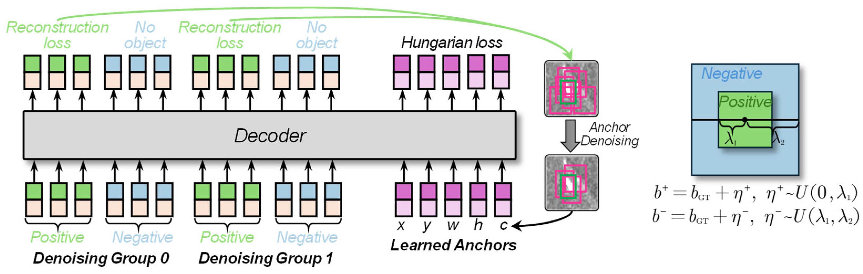
CDN-FD integrates a comparative learning mechanism that leverages positive–negative sample pairs to enhance feature discrimination, inspired by [26], simultaneously improving convergence speed and spatial resolution in ship target detection tasks. Figure 9 shows its schematic diagram. Two types of perturbed samples are generated for each ground truth box by

$$b^{+}=b_{\mathrm{GT}}+{\eta }^{+}, {\eta }^{+}~U\left(0,{\lambda }_1\right)$$

(33)

$$b^{-}=b_{\mathrm{GT}}+{\eta }^{-}, {\eta }^{-}~U\left({\lambda }_1,{\lambda }_2\right)$$

(34)

where $b_{\mathrm{GT}}$ denotes the ground truth box, $b^{+}$ denotes the positive box with a noise disturbance parameter ${\eta }^{+}$, $b^{-}$ denotes the positive box with a noise disturbance parameter ${\eta }^{-}$, and ${\lambda }_1$ and ${\lambda }_2$ denote two thresholds for positive and negative samples, which are set to 0.1 and 0.7 empirically. $U$ denotes uniform sampling. Additionally, dynamic gradient filtering is used, i.e., the gradient is updated only for positive samples with $\mathrm{IoU}>0.3$ to prevent invalid noise interference. In this way, the reconstruction process can be expressed as

$$L\left(\theta ,\varphi \right)={\displaystyle \frac{1}{N}}{\displaystyle \sum _{i=1}^N\Vert b_{\mathrm{GT}}-D_{\theta }{E}_{\varphi }\left(b_{\mathrm{GT}}\right){\Vert }_2^2}$$

(35)

where $E_{\varphi }$ represents the addition of noise with the parameter $\varphi$ and $D_{\theta }$ represents the denoising with the parameter $\theta$. Within the denoising architecture, the one-to-many label assignment paradigm significantly boosts training supervision, simultaneously boosting convergence speed and preserving detection integrity. The paired original and noisy queries are processed through grouped representations, where each cluster undergoes independent self-attention learning. An attention masking scheme creates isolated processing environments, rendering inter-group connections inactive (represented as matrix gray zones) while maintaining intra-group communication. This controlled visibility protocol ensures strict one-way interaction between query types, thereby safeguarding against any inference-phase information leakage. As a result, the training optimization objective is defined as follows:

$$L={\lambda }_{\mathrm{reg}}\Vert b^{+}-b_{\mathrm{GT}}{\Vert }_1+{\lambda }_{\mathrm{cls}}J\left(b^{+},y_{\mathrm{GT}}\right)+{\lambda }_{\mathrm{neg}}\max \left(0,\sigma -p^{-}\right)$$

(36)

where $J\left(\cdot \right)$ is the cross-entropy, $\sigma$ is a negative threshold set to 0.3, and ${\lambda }_i$ denotes different weight coefficients. ${\lambda }_{\mathrm{reg}}$, ${\lambda }_{\mathrm{cls}}$ and ${\lambda }_{\mathrm{neg}}$ are set to 1.0, 2.0, and 0.5 empirically. Taking ${\lambda }_{\mathrm{reg}}$ as the reference weight, ${\lambda }_{\mathrm{cls}}$ is increased to emphasize category discrimination, whereas ${\lambda }_{\mathrm{neg}}$ is reduced so that negative-sample suppression acts as an auxiliary constraint without dominating the optimization. CDN-FD leverages contrastive learning to explicitly differentiate between valid targets and noisy anchor boxes, eliminating reliance on the unstable Hungarian matching algorithm. By directly establishing robust correlations between queries and ground truth instances, this approach bypasses intermediate optimization steps, ensuring more precise and stable learning dynamics.

4. Experiments

4.1. Data Description

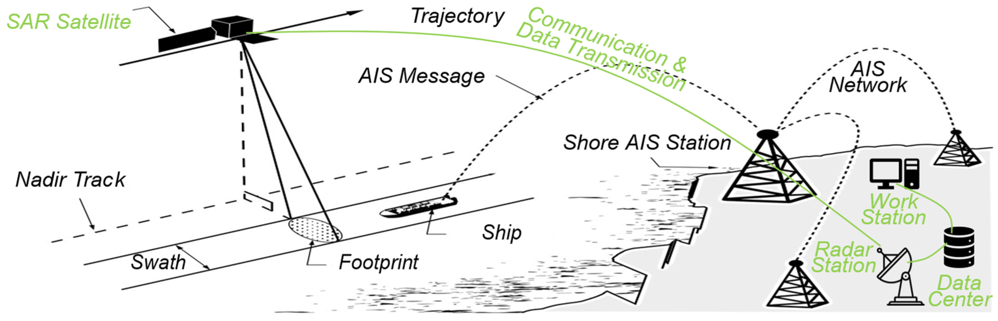
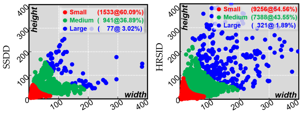
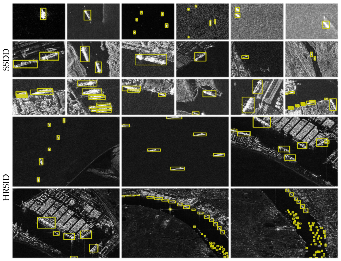
As shown in

Table 3. System parameters of spaceborne SAR instruments used in this work.

Satellite	Agent	Date	Height	Band	Bandwidth (MHz)	Polarization	Res.
RadarSat-2	CSA	2007~	798 km	C	11.6/17.3/30.0	HH/HV/VH/VV	1~100 m
TerraSAR-X	DLR	2007~	515 km	X	150/300	VV/HH, HH/VV	0.25~40 m
Sentinel-1	ESA	2014~	693 km	C	100	HH, VH, HV, VV	1~25 m

, the marine ship surveillance system integrates data from three distinct SAR platforms: RadarSat-2 (C-band, 1 m resolution, 2007), TerraSAR-X (X-band, 0.25 m spotlight mode, 2007), and Sentinel-1 (C-band constellation, 2014, full polarization). As illustrated in Figure 10, the operational pipeline involves ground radar stations receiving satellite data, centralized storage in data centers, and subsequent workstation access for data processing. Validation employs an automatic identification system (AIS) as a ground truth reference. As shown in Figure 11 and

Table 4. Data summary of SSDD and HRSID.

Data	#All	#Train	#Test	#Ship	#ShipS	#ShipM	#ShipL	Polarization	Resolution	Satellite
SSDD	1160	928	232	2551	1533	941	77	HH, HV, VV, VH	1~5 m	TerraSAR-X, RadarSat-2
HRSID	5604	3642	1962	16,965	9256	7388	321	HH, HV, VV	0.5~3 m	Sentinel-1, TerraSAR-X

, two standardized datasets are utilized—the SAR ship detection dataset (SSDD) [28], comprising 1160 images with 2551 ships, and the more extensive high-resolution SAR image dataset (HRSID) [29], containing 5604 images with 16,965 ships. Both datasets maintain consistent training–test splits with prior studies. The practical engineering verification employs two large-scale Sentinel-1 SAR images (denoted as LSS1 and LSS2) as primary testbeds. To further substantiate method efficacy, an additional evaluation is conducted using the SAR-Ship-Dataset [30] and SARDet-100K [31] repositories. Cross-domain validation is achieved through optical and infrared ship datasets, including HRSC [5] and ISDD [7], systematically assessing TLTA’s generalization capacity across modalities.

4.2. Experimental Configuration

We employ SGD over 320 epochs with dynamic learning rate scheduling: starting at 0.04 and reduced by 10× at milestones 280 and 300. The optimization strategy integrates Nesterov momentum (0.99) with L2 regularization (0.005 attenuation). Batch size configurations account for memory constraints, setting 4 for SSDD (800 × 800) and 2 for HRSID (1024 × 1024). Execution hardware comprises an NVIDIA RTX 5090 GPU and an Intel Ultra-9 CPU. The spectral hypergraph convolution adopts a first-order Chebyshev approximation ($K=1$), and CACN contains five cross-attention blocks. In CDN-FD, the positive and negative perturbation thresholds are set to 0.1 and 0.7, respectively; the negative threshold is set to 0.3, and ${\lambda }_{\mathrm{reg}}$, ${\lambda }_{\mathrm{cls}}$ and ${\lambda }_{\mathrm{neg}}$ are set to 1.0, 2.0, and 0.5, respectively. Under this configuration, training the complete TLTA requires approximately 0.29 s per image for training with a peak GPU memory usage of 28 GB. The complete model contains 55 M parameters and requires 33 ms per image for inference. The source code is made publicly available at https://github.com/RUIZHU1217/TLTA (accessed on 9 September 2026).

4.3. Evaluation Metrics

For benchmark experiments, the COCO evaluation criterion is adopted, whose average precision (AP) is defined by

$$\mathrm{AP}={\displaystyle {\int }_0^{1}p\left(r\right)\mathrm{d}r} \mathrm{where} p={\displaystyle \frac{\mathrm{TP}}{\mathrm{TP}+\mathrm{FP}}}, r={\displaystyle \frac{\mathrm{TP}}{\mathrm{TP}+\mathrm{FN}}}$$

(37)

where TP, FP, and FN are the numbers of true positives, false positives, and false negatives. The values of AP at different IoU thresholds are denoted by ${\mathrm{AP}}_{50}$ and ${\mathrm{AP}}_{75}$. The values of AP at different scales are denoted by ${\mathrm{AP}}_{\mathrm{S}}$, ${\mathrm{AP}}_{\mathrm{M}}$ and ${\mathrm{AP}}_{\mathrm{L}}$. These scale-aware metrics are informative when the evaluated dataset contains targets over multiple size ranges. For the large-scene experiments, all ship instances fall within the small-target range. Therefore, scale-specific AP metrics provide limited additional information, and a VOC-style evaluation protocol with an IoU threshold of 0.5 is adopted, with ${\mathrm{AP}}_{50}$ used as the AP metric. When checking false alarms and missed detections, the harmonic average $f1$ is used, which is calculated by $2\left(p\times r\right)/\left(p+r\right)$.

5. Results

5.1. Quantitative Results

5.1.1. Method Comparison

The quantitative results shown in

Table 5. Quantitative comparison on SSDD and HRSID. The best is marked in magenta. The second-best is marked in blue. The results that exceed the previous best are marked in bold.

Method		SSDD						HRSID
		AP	AP50	AP75	APS	APM	APL	AP	AP50	AP75	APS	APM	APL
2021 Sparse R-CNN [21]		69.7	96.6	83.8	72.1	60.7	69.6	69.4	92.2	81.5	70.8	68.8	39.3
2021 Conditional DETR [23]		70.8	96.5	86.5	72.7	66.5	43.9	68.7	91.7	79.3	69.5	69.0	43.4
2022 Anchor DETR [24]		71.1	97.1	85.1	72.0	69.9	62.6	70.9	92.8	82.9	72.6	71.5	31.7
2022 DN-DETR [25]		70.4	97.8	85.0	70.5	71.3	69.2	69.4	92.0	81.2	70.8	68.6	21.8
2022 ICFM [35]		61.3	96.6	72.9	59.3	66.5	45.3	60.6	85.5	67.9	61.4	65.5	32.0
2023 DiffusionDet [20]		67.2	93.9	82.6	67.4	66.7	70.5	66.0	88.6	80.5	70.8	66.9	28.4
2023 DINO [26]		73.1	96.9	89.1	72.4	76.5	72.3	71.2	91.6	80.9	73.0	71.1	10.0
2023 DAB-DETR [27]		72.6	97.7	90.1	73.3	72.0	68.6	70.2	91.5	80.8	72.0	68.5	11.7
2023 FBUA-Net [36]		63.9	96.2	77.6	59.9	75.1	75.4	69.1	90.3	79.6	69.6	66.4	50.2
2024 CLFR-Det [37]		72.0	97.8	87.1	72.0	73.8	65.8	68.8	91.1	79.5	71.3	64.0	25.5
2024 RT-DETR [58]		73.0	97.2	88.4	72.4	76.0	64.1	70.8	92.2	82.1	71.8	71.6	40.1
2024 MS-DETR [59]		74.4	98.0	90.6	73.8	73.9	63.0	72.3	92.2	83.9	73.9	70.0	21.5
2024 DQ-DETR [60]		73.0	98.3	89.6	73.0	74.2	58.1	72.8	92.8	83.0	74.6	69.2	25.0
2025 Hyper-YOLO [14]		73.7	97.4	90.1	74.0	73.3	58.1	71.7	92.1	83.0	73.3	69.2	26.6
2025 LSNet [61]		74.1	98.5	91.3	73.7	76.5	63.2	72.5	92.7	82.7	74.0	69.9	25.0
2025 EViT [62]		71.9	97.6	88.8	72.4	71.7	55.5	71.7	91.0	83.3	73.1	70.9	30.5
2025 FDI-YOLO [77]		70.8	98.4	86.7	70.3	70.3	68.7	67.0	91.0	74.8	68.4	68.9	33.6
2025 GFNet [78]		72.2	97.8	86.8	72.1	74.3	49.9	71.9	92.9	83.0	73.1	67.1	23.1
2025 RDB-DINO [79]		74.7	98.3	90.5	73.4	--	--	71.8	92.8	82.4	72.5	--	--
2026 TLSA [52]		78.1	98.7	94.9	77.4	83.5	75.0	75.4	94.8	86.0	75.8	73.5	44.5
Baseline		72.2	96.4	87.6	73.4	70.9	68.3	68.9	88.2	79.2	70.5	63.8	22.0
TLTA	i-LTA	74.1	97.2	90.5	74.1	76.0	71.0	71.6	89.4	81.8	73.0	68.8	28.2
	i-LTA + f-LTA	75.2	98.5	91.1	75.0	78.9	80.2	74.9	91.8	84.6	77.1	70.3	34.9
	i-LTA + f-LTA + p-LTA	77.9	98.8	93.2	78.0	84.2	82.8	76.4	93.4	85.2	78.5	73.0	51.8
Better than Baseline		+5.7	+2.4	+5.6	+4.6	+13.3	+14.5	+7.5	+5.2	+6.0	+8.0	+9.2	+29.8
than Previous Best		−0.2	+0.1	−1.7	+0.6	+0.7	+7.4	+1.0	−1.4	−0.8	+2.7	−0.5	+1.6

compare TLTA with recent SAR ship detection methods. All methods are compared on the same benchmark datasets using the same evaluation metrics, while architecture-specific training configurations are retained where applicable. TLTA achieves AP values of 77.9% and 76.4% on SSDD and HRSID, respectively. Compared with TLSA, TLTA is 0.2% lower in AP on SSDD but 1.0% higher on HRSID. It also achieves higher ${\mathrm{AP}}_{\mathrm{S}}$ and ${\mathrm{AP}}_{\mathrm{L}}$ on both datasets and higher ${\mathrm{AP}}_{\mathrm{M}}$ on SSDD. The improvement can be largely attributed to the hierarchical topology modeling strategy of TLTA. Unlike DETR- and Transformer-based detectors that primarily model pairwise interactions through attention, TLTA employs hypergraphs to capture high-order relationships among multiple entities. Compared with recent SAR ship detection methods that mainly enhance feature representation, multi-scale information, or detection heads, TLTA progressively introduces topology awareness at the input, feature, and proposal levels. Moreover, compared with hypergraph-enhanced detectors such as Hyper-YOLO, TLTA extends hypergraph modeling across multiple stages of the detection pipeline rather than restricting it to feature representation alone.

5.1.2. Quantitative Analysis of TLTA Efficacy

The multi-level topology awareness in TLTA demonstrates substantial performance enhancements, as quantitatively shown in Table 5. The baseline refers to the basic detection framework without the proposed i-LTA, f-LTA, and p-LTA modules, compared with which the complete TLTA improves AP by 5.7 and 7.5 percentage points on SSDD and HRSID, respectively. This advancement stems from the super-pixel hypergraph computation enhancing input representation of i-LTA, the feature hypergraph modeling intricate semantic–spatial relationships of f-LTA, and the proposal hypergraph learning inter-ship spatial patterns of p-LTA, thereby collectively forming a synergistic high-order topological learning system.

5.2. Qualitative Results

5.2.1. Surveillance Visualization

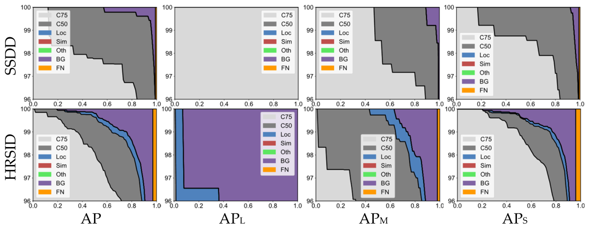
The qualitative results presented in Figure 12 illustrate TLTA’s detection performance across diverse maritime scenarios. The method consistently identifies various ships with high precision in both offshore and complex coastal environments. It also maintains stable detection for isolated ships, densely distributed targets, and ships with different scales, despite variations in background clutter, target density, and scene complexity. Additionally, the precision–recall curves in Figure 13 remain close to the upper-left region across the overall and scale-specific evaluations, further demonstrating the consistent detection performance of TLTA.

5.2.2. Qualitative Analysis of TLTA Efficacy

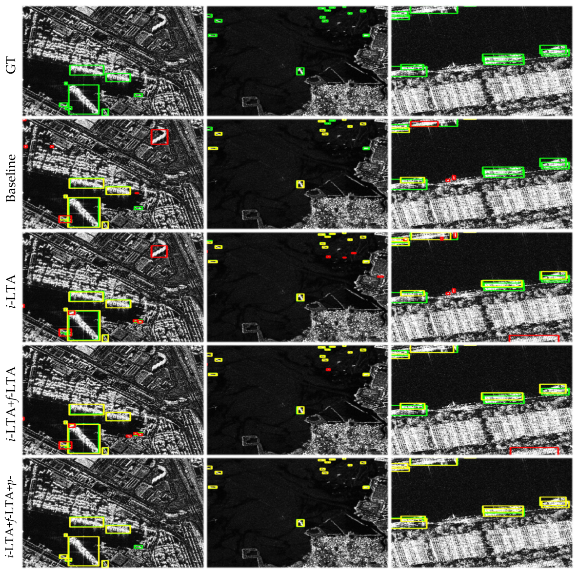
Figure 14 provides visual evidence of the surveillance performance evolution of TLTA with stepwise increasing topology awareness. The surveillance results demonstrate progressive improvement across different scenes, with a reduction in false positives and recovery of previously missed detections. In particular, the successive introduction of i-LTA, f-LTA, and p-LTA gradually improves the consistency between the predicted and ground-truth ship locations, especially in complex coastal regions and densely distributed ship scenes. This progressive enhancement pattern further supports the effectiveness of multi-level topology awareness in TLTA.

5.2.3. Failure Cases

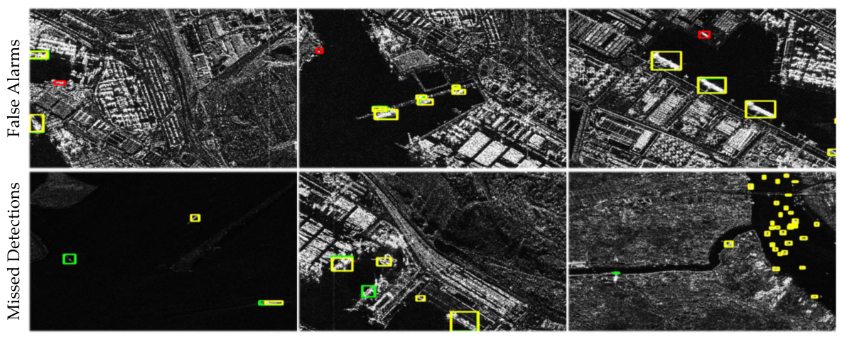
Figure 15 shows some representative failure cases that highlight potential avenues for methodological refinement. Notably, certain small metallic reflections along coastal regions are erroneously classified as ships, likely attributable to insufficiently distinct topological contextual cues in these regions. Additionally, several low-signature small ships remained undetected, potentially due to their subtle electromagnetic responses being obscured by environmental noise. These isolated detection anomalies occur with infrequency, so their impact on the overall efficacy remains negligible, as demonstrated by the aforementioned consistently high-performance metrics on diverse operational scenarios. These observations suggest that future work should prioritize boosting feature discriminability through improved feature extraction techniques.

6. Analysis and Discussion

6.1. Further Analysis

6.1.1. Continuous Enhancement in Complex Scenes

The experimental results presented in

Table 6. Performance evaluation of TLTA on inshore and offshore scenes.

Method		SSDD						HRSID
		Inshore			Offshore			Inshore			Offshore
		AP	AP50	AP75	AP	AP50	AP75	AP	AP50	AP75	AP	AP50	AP75
Baseline		64.1	93.5	77.8	71.9	98.1	90.2	51.2	76.0	60.5	81.3	97.0	94.0
TLTA	i-LTA	68.9	95.6	83.5	74.1	98.3	92.6	58.6	82.4	63.7	82.0	97.5	94.2
	i-LTA + f-LTA	73.4	97.7	89.3	77.8	98.6	93.9	61.5	84.2	69.8	83.9	98.1	94.8
	i-LTA + f-LTA + p-LTA	77.8	98.2	92.0	79.0	98.7	95.0	64.8	87.8	72.6	85.0	98.2	95.1
Better than Baseline		+13.7	+4.7	+14.2	+7.1	+0.6	+4.8	+13.6	+11.8	+12.1	+3.7	+1.2	+1.1
SSDD
HRSID

demonstrate that the proposed higher-order topological awareness framework provides more pronounced improvements over the baseline in complex inshore scenarios than in pure maritime offshore environments. This observation demonstrates the effectiveness of TLTA in modeling intricate spatial relationships between ships and surrounding infrastructure elements, including berthing structures, cargo handling systems, and terrestrial installations. The stronger improvement in inshore scenes suggests that topology-aware modeling is particularly beneficial when ship targets coexist with complex shoreline structures, where distinguishing ships in proximity to docks, gantries, and other land-based structures has traditionally resulted in higher error rates. The progressive topological learning framework of TLTA helps reduce the performance degradation caused by complex coastal backgrounds and improves detection reliability in such environments.

Table 7. Performance gap between inshore and offshore on SSDD.

Method	Inshore	Offshore	∆	Visualization
	AP50	AP50
FBR-Net [40]	80.1	96.4	−16.3
FSTSE [41]	82.0	98.3	−16.3
RFEM [42]	83.6	99.7	−16.1
ELLK-Net [43]	87.2	97.8	−10.6
FINet [44]	90.5	99.8	−9.3
HRLE-SARDet [45]	93.1	99.1	−6.0
CSnNet [46]	95.1	98.8	–3.7
TLTA	98.2	98.7	−0.7

further shows that TLTA substantially narrows the accuracy disparity between inshore and offshore scenes on SSDD compared with the other methods. This demonstrates TLTA’s ability to maintain more consistent detection performance across different maritime environments.

6.1.2. Reliable False Alarm Suppression

Table 8. Evaluation of false alarms and missed detections.

Method		SSDD			HRSID			Visualization
		p	r	f1	p	r	f1
Baseline		94.1	95.8	94.9	90.3	89.3	89.8
TLTA	i-LTA	95.8	96.9	96.3	91.5	90.4	90.9
	i-LTA + f-LTA	97.2	97.6	97.4	93.2	91.0	92.1
	i-LTA + f-LTA + p-LTA	98.0	98.5	98.2	94.0	91.2	92.6
Better Than Baseline		+3.9	+2.7	+3.3	+3.7	+1.9	+2.8

shows that higher-order topology awareness credibly suppresses false alarms while maintaining detection sensitivity. The observed $p\text{-}r$ trade-off reveals a systematic reduction in both false positives and missed detections, culminating in improved $f1$ scores. This dual optimization stems from the capacity of TLTA to integrate global contextual information through advanced feature representation, complemented by the cross-attention mechanism in i-LTA for preserving critical local details.

6.1.3. Discriminative Feature Extraction

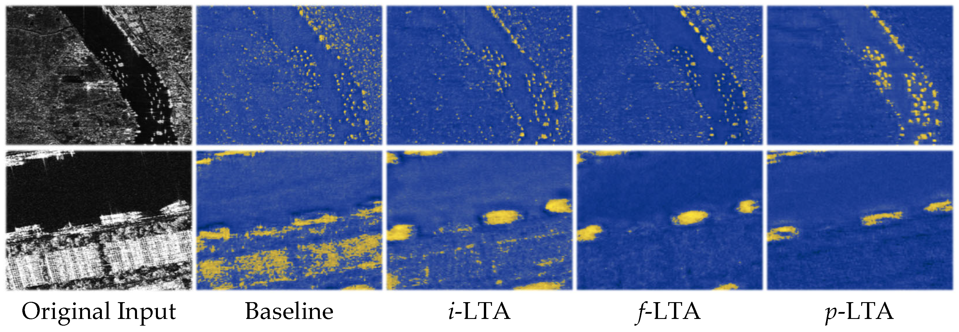
TLTA enables discriminative feature extraction as shown in Figure 16. The observed transition in feature map characteristics—where ship contours sharpen, and land signatures fade—provides empirical evidence of topology awareness’s discriminative power. This spatial filtering effect directly correlates with improved detection performance, as the framework learns to prioritize salient maritime features while suppressing irrelevant land-based patterns through adaptive feature selection.

6.1.4. Concentrated Feature Activation

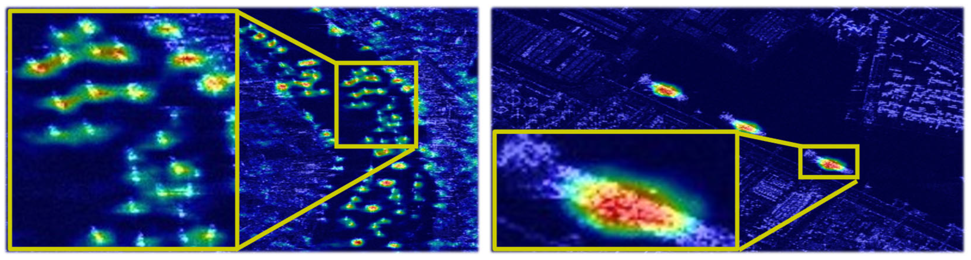
The feature activation states visualized in Figure 17 reveal that TLTA demonstrates selective attention allocation, with predominant activation concentrated on ship regions. This targeted activation mechanism directly contributes to improved detection accuracy, as the framework’s high-order topology awareness enables precise identification of semantically significant maritime areas through comprehensive scene interpretation.

6.1.5. Complexity Analysis

The complexity evaluation in

Table 9. Complexity analysis.

Method		#Para	GFLOPs	t/ms	FPS	Visualization
RT-DETR [58]		76 M	259	33	30
DAFDet [47]		91 M	173	31	32
RDB-DINO [79]		64 M	298	38	27
M2S-DETR [48]		67 M	239	37	27
Baseline		38 M	138	28	36
TLTA	i-LTA	43 M	169	29	34
	i-LTA + f-LTA	48 M	254	31	32
	i-LTA + f-LTA + p-LTA	55 M	286	33	30

shows that progressively introducing topology awareness increases the computational cost, with the full TLTA requiring 55 M parameters and 286 GFLOPs compared with 38 M parameters and 138 GFLOPs for the baseline. However, the inference time increases only from 28 ms to 33 ms, while the throughput decreases from 36 FPS to 30 FPS. Compared with representative mainstream detectors, the full TLTA remains within a comparable range of model size and inference efficiency, achieving 30 FPS under the adopted hardware configuration. These results indicate that the additional computation introduced by multi-level topology modeling is accompanied by consistent accuracy improvements while maintaining competitive inference efficiency. Therefore, TLTA provides a reasonable trade-off between detection accuracy and computational cost for maritime surveillance, although deployment efficiency may vary with hardware platforms and image resolution.

6.1.6. Ablation Studies

The systematic ablation studies conducted on several core modules in TLTA, including CACN, VL-FSA, EL-FSA, DCFE, and proposal hypergraphs, evaluate their individual contributions to the overall performance. As shown in

Table 10. Evaluation of CACN. ✓ indicates that the corresponding input/module is included, whereas ✗ indicates that it is not included.

$\mathcal{I}$	${\mathcal{I}}_{SP}$	Operation	AP
✓	✗	--	75.3
✓	✓	Concatenate	75.8
✓	✓	CACN	76.4

, combining the spectral and spatial branches improves the AP from 75.3% to 75.8%, while CACN further increases it to 76.4%. This improvement mainly benefits from the complementary topology information captured by the two branches: the spectral branch models high-order structural correlations, whereas the spatial branch propagates vertex–hyperedge–vertex interactions along hyperpaths. Their parallel combination therefore provides a more comprehensive topology representation, while CACN further integrates the topology-aware representation with low-level spatial details.

Table 11. Evaluation of VL-FSA and EL-FSA. ✓ indicates that the corresponding input/module is included, whereas ✗ indicates that it is not included.

VL-FSA	EL-FSA	AP
✗	✗	74.9
✓	✗	75.6
✓	✓	76.4

shows that introducing VL-FSA improves the AP from 74.9% to 75.6%, and jointly using VL-FSA and EL-FSA further increases it to 76.4%, demonstrating the benefit of jointly exploiting vertex- and hyperedge-level information. As shown in

Table 12. Evaluation of DCFE. ✓ indicates that the corresponding input/module is included, whereas ✗ indicates that it is not included.

DCFE	AP
✗	76.0
✓	76.4

, DCFE improves the AP from 76.0% to 76.4%, confirming its contribution to feature enhancement. Furthermore,

Table 13. Evaluation of proposal hypergraphs.

Type	AP
One Pathway (P-HGC)	75.9
Two Pathways (PP-HGC + NP-HGC)	76.4

shows that the two-pathway proposal hypergraph design improves the AP from 75.9% to 76.4% compared with the one-pathway counterpart, indicating the effectiveness of jointly modeling positive and negative proposal features.

6.2. Discussion

6.2.1. Large Scene Verification Towards Practical Engineering

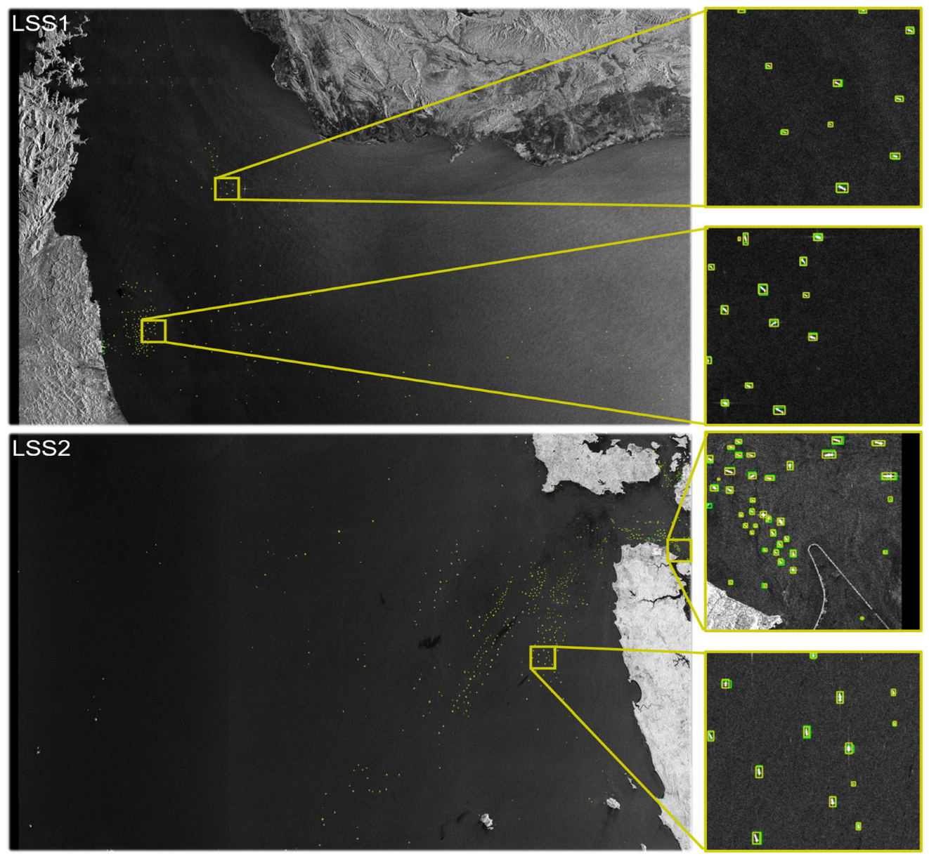
The large-scale evaluation using Sentinel-1 SAR data, as shown in

Table 14. Data description of two large-scene Sentinel-1 SAR images.

Image	Time	Location	Polarization	Mode	Resolution	Image Size	Ships
LSS1	6 June 2020	Singapore Strait	VV	IW	5 m × 20 m	25,650 × 16,786	760
LSS2	18 June 2020	Gulf of Cadiz	VV	IW	5 m × 20 m	25,644 × 16,722	351

, demonstrates the robust performance of TLTA in real-world marine surveillance applications. The two large scenes cover different maritime environments and ship distributions, including both sparsely distributed targets and densely clustered ships near coastal regions. The qualitative results in Figure 18 and quantitative metrics in

Table 15. Evaluation of two large-scene Sentinel-1 SAR images.

Method	LSS1									LSS2
	GT	Det	TP	FP	FN	r	p	AP50	f1	GT	Det	TP	FP	FN	r	p	AP50	f1
SE-Rank [32]	760	678	599	79	161	88.4	78.8	77.3	83.3	351	323	291	32	60	90.1	82.9	81.9	86.4
DAPN [33]	760	707	616	91	144	87.1	81.1	78.8	84.0	351	335	292	43	59	87.2	83.2	82.4	85.2
HRSDNet [29]	760	509	490	19	270	96.3	64.5	63.8	77.3	351	264	256	8	95	97.0	72.9	72.5	83.2
ARPN [34]	760	712	620	92	140	87.1	80.1	79.0	83.5	351	348	298	53	62	85.6	82.8	81.1	84.2
TP-CFAR [9]	760	863	603	260	157	69.9	79.3	--	74.3	351	556	314	242	37	56.5	89.5	--	69.3
TLTA	760	750	648	102	112	85.3	86.4	81.2	85.8	351	345	316	29	35	90.0	91.6	85.7	90.8

collectively confirm TLTA’s capability to maintain detection accuracy across extensive ocean areas. In particular, TLTA achieves AP50 values of 81.2% and 85.7%, and f1 scores of 85.8% and 90.8% on LSS1 and LSS2, respectively. These results further support the applicability of TLTA to large-scene ship surveillance across diverse large-scale maritime environments under different target densities and background conditions.

6.2.2. Validation on Large-Scale Datasets

To further substantiate the efficacy of TLTA, an additional evaluation is conducted on SAR-Ship-Dataset [30] and SARDet-100K [31]. SAR-Ship-Dataset contains 43,819 image samples, while SARDet-100K contains 116,598 image samples. The results are shown in

Table 16. Validation results on two large-scale datasets.

SAR-Ship-Dataset [30]				SARDet-100K [31]
Method		AP	AP50	Method		AP	AP50
YOLOX [15]		67.7	93.1	YOLOX [15]		34.1	66.8
LRTransDet [49]		--	95.1	TOOD [81]		54.7	86.9
SRDet [50]		65.9	95.1	VFNet [82]		53.0	84.3
ESA-CDH-WIL [51]		72.1	94.5	DenoDet [83]		55.9	85.8
Baseline		66.8	92.6	Baseline		52.6	83.1
TLTA	i-LTA	69.5	94.0	TLTA	i-LTA	53.5	85.4
	i-LTA + f-LTA	73.7	95.2		i-LTA + f-LTA	55.8	87.7
	i-LTA + f-LTA + p-LTA	75.8	96.5		i-LTA + f-LTA + p-LTA	56.9	89.1

. The experimental results demonstrate TLTA’s consistent effectiveness across diverse operational scenarios, achieving consistent improvements over the baseline and competitive performance compared with representative methods. This sustained efficacy underscores the fundamental stability and practical value of topology awareness as a core architectural principle.

6.2.3. Domain Expansion Exploration

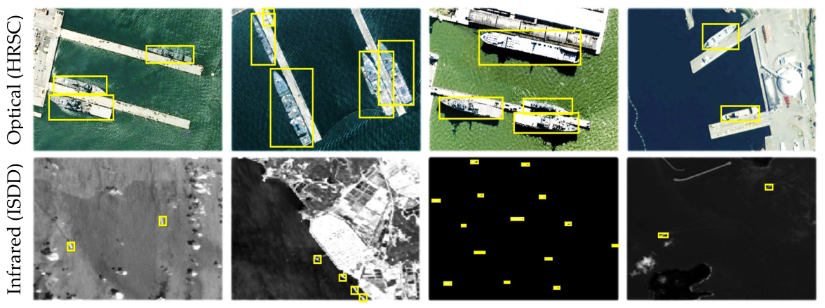
Last but not least, the evaluation on heterogeneous datasets, including HRSC optical imagery and ISDD infrared collections, is used to confirm TLTA’s robust cross-domain applicability. The results shown in

Table 17. Evaluation of optical and infrared domains. The best performance is marked in bold.

Optical (HRSC [5])				Infrared (ISDD [7])
Method		AP	AP50	Method		AP	AP50
DAB-DETR [27]		59.0	89.9	Sparse R-CNN [21]		41.5	89.7
CM-YOLO [4]		61.5	91.4	KCPNet [7]		42.6	91.0
Baseline		58.5	87.6	Baseline		38.9	87.3
TLTA	i-LTA	60.8	90.4	TLTA	i-LTA	41.7	89.8
	i-LTA + f-LTA	62.3	92.0		i-LTA + f-LTA	43.8	92.6
	i-LTA + f-LTA + p-LTA	63.5	93.8		i-LTA + f-LTA + p-LTA	44.9	94.2

and Figure 19 demonstrate that topology learning maintains effective detection performance across different spectral bands, indicating its potential beyond SAR imagery. On both optical and infrared datasets, progressively introducing i-LTA, f-LTA, and p-LTA consistently improves the detection results over the corresponding baseline. The qualitative examples further show that TLTA can identify ships under substantially different imaging characteristics and background appearances. These results suggest that the proposed topology-aware modeling strategy is not restricted to a single sensing modality and can retain its effectiveness across heterogeneous ship surveillance domains.

6.2.4. Limitations and Future Work

Although TLTA achieves consistent improvements across different SAR ship detection scenarios, several limitations remain. As shown in Figure 15, false alarms may occur in complex coastal regions where strong metallic scatterers resemble ships, while low-signature small ships can still be missed when their weak responses are obscured by speckle or environmental noise. These cases indicate that topology modeling remains dependent on the discriminability of the underlying features. Future work will focus on improving topology construction under complex backgrounds and weak-target conditions. More discriminative contextual representations and enhanced weak-target feature extraction will be explored to better distinguish ships from ship-like scatterers and improve small-ship detection. Adaptive topology construction may further suppress unreliable relationships and improve robustness in challenging maritime environments.

7. Conclusions

We explore topology awareness for SAR marine ship surveillance through a hypergraph framework with three hierarchical levels. The proposed TLTA framework integrates the input-level (i-LTA), feature-level (f-LTA), and proposal-level (p-LTA) mechanisms to progressively extract high-order spatial topology representations. Extensive experiments demonstrate that topology awareness improves SAR ship surveillance performance while maintaining cross-sensor adaptability to optical and infrared modalities. TLTA offers competitive accuracy with computational efficiency comparable to mainstream alternatives. Our work demonstrates the potential of high-order topology modeling using hypergraphs for SAR marine ship surveillance.

References

1. Liu, S.; Li, D.; Song, H.; Fan, C.; Li, K.; Wan, J.; Liu, R. SAR ship detection across different spaceborne platforms with confusion-corrected self-training and region-aware alignment framework. ISPRS J. Photogramm. Remote Sens. 2025, 228, 305–322. [Google Scholar] [CrossRef] [Scilit]
2. Zhang, T.; Gao, G.; Zhang, X. Glance-Focus-Gaze: A Novel Eagle-Eye Vision-Inspired Panorama-Population-Individual Progressive Screening Paradigm to Capture Ships in SAR Images. ISPRS J. Photogramm. Remote Sens. 2026, 235, 241–260. [Google Scholar] [CrossRef] [Scilit]
3. Gao, G.; Bai, Q.; Zhang, C.; Zhang, L.; Yao, L. Dualistic cascade convolutional neural network dedicated to fully PolSAR image ship detection. ISPRS J. Photogramm. Remote Sens. 2023, 202, 663–681. [Google Scholar] [CrossRef] [Scilit]
4. Min, L.; Dou, F.; Zhang, Y.; Shao, D.; Li, L.; Wang, B. CM-YOLO: Context modulated representation learning for ship detection. IEEE Trans. Geosci. Remote Sens. 2025, 63, 4202414. [Google Scholar] [CrossRef] [Scilit]
5. Liu, Z.; Yuan, L.; Weng, L.; Yang, Y. A high resolution optical satellite image dataset for ship recognition and some new baselines. In Proceedings of the 6th International Conference on Pattern Recognition Applications and Methods (ICPRAM), Porto, Portugal, 24–26 February 2017; Volume 1, pp. 324–331. [Google Scholar]
6. Xu, X.; Zhang, X.; Wei, S.; Shi, J.; Zhang, W.; Zhang, T.; Zhan, X.; Xu, Y.; Zeng, T. DiffSARShipInst: Diffusion model for ship instance segmentation from synthetic aperture radar imagery. ISPRS J. Photogramm. Remote Sens. 2025, 223, 440–455. [Google Scholar] [CrossRef] [Scilit]
7. Han, Y. Knowledge-driven context perception for ship detection in infrared imagery. IEEE Trans. Geosci. Remote Sens. 2023, 61, 5000219. [Google Scholar] [CrossRef] [Scilit]
8. Wu, B.; Liu, C.; Chen, J. A review of spaceborne high-resolution spotlight/sliding spotlight mode SAR imaging. Remote Sens. 2024, 17, 38. [Google Scholar] [CrossRef] [Scilit]
9. Kronauge, M.; Rohling, H. Fast two-dimensional CFAR procedure. IEEE Trans. Aerosp. Electron. Syst. 2013, 49, 1817–1823. [Google Scholar] [CrossRef] [Scilit]
10. Zhang, T.; Zhang, X.; Liu, C.; Shi, J.; Wei, S.; Ahmad, I.; Zhan, X.; Zhou, Y.; Pan, D.; Li, J.; et al. Balance learning for ship detection from synthetic aperture radar remote sensing imagery. ISPRS J. Photogramm. Remote Sens. 2021, 182, 190–207. [Google Scholar] [CrossRef] [Scilit]
11. Zhang, T.; Zhang, X.; Shi, J.; Wei, S. HyperLi-Net: A hyper-light deep learning network for high-accurate and high-speed ship detection from synthetic aperture radar imagery. ISPRS J. Photogramm. Remote Sens. 2020, 167, 123–153. [Google Scholar] [CrossRef] [Scilit]
12. LeCun, Y.; Bengio, Y.; Hinton, G. Deep Learning. Nature 2015, 521, 436–444. [Google Scholar] [CrossRef] [Scilit] [PubMed]
13. Ren, S.; He, K.; Girshick, R.; Sun, J. Faster R-CNN: Towards real-time object detection with region proposal networks. In Proceedings of the Advances in Neural Information Processing Systems (NeurIPS/NIPS), Montréal, QC, Canada, 7–12 December 2015; Volume 28, pp. 91–99. [Google Scholar]
14. Feng, Y.; Huang, J.; Du, S.; Ying, S.; Yong, J.H.; Li, Y.; Ding, G.; Ji, R.; Gao, Y. Hyper-YOLO: When visual object detection meets hypergraph computation. arXiv 2024, arXiv:2408.04804. [Google Scholar]
15. Ge, Z.; Liu, S.; Wang, F.; Li, Z.; Sun, J. YOLOX: Exceeding YOLO series in 2021. arXiv 2021, arXiv:2107.08430. [Google Scholar]
16. Melillos, G.; Hadjimitsis, D.G. Ship detection using SAR images based on YOLO at Cyprus’s coast. In Proceedings of the SPIE Geospatial Informatics XII, Orlando, FL, USA, 27 May 2022; Volume 12099, p. 1209903. [Google Scholar]
17. Liu, W.; Anguelov, D.; Erhan, D.; Szegedy, C.; Reed, S.; Fu, C.-Y.; Berg, A.C. SSD: Single Shot MultiBox Detector. In Computer Vision—ECCV 2016, Lecture Notes in Computer Science; Springer: Cham, Switzerland, 2016; Volume 9905, pp. 21–37. [Google Scholar]
18. Lin, T.Y.; Dollár, P.; Girshick, R.; He, K.; Hariharan, B.; Belongie, S. Feature Pyramid Networks for Object Detection. In Proceedings of the IEEE Conference on Computer Vision and Pattern Recognition (CVPR), Honolulu, HI, USA, 21–26 June 2017; pp. 936–944. [Google Scholar]
19. Duan, K.; Bai, S.; Xie, L.; Qi, H.; Huang, Q.; Tian, Q. CenterNet: Keypoint Triplets for Object Detection. In Proceedings of the IEEE/CVF International Conference on Computer Vision (ICCV), Seoul, Republic of Korea, 27 October–2 November 2019; pp. 6569–6578. [Google Scholar]
20. Chen, S.; Sun, P.; Song, Y.; Luo, P. DiffusionDet: Diffusion model for object detection. In Proceedings of the IEEE/CVF International Conference on Computer Vision (ICCV), Paris, France, 1–6 October 2023; pp. 19830–19843. [Google Scholar]
21. Sun, P.; Zhang, R.; Jiang, Y.; Kong, T.; Xu, C.; Zhan, W.; Tomizuka, M.; Li, L.; Yuan, Z.; Wang, C.; et al. Sparse R-CNN: End-to-end object detection with learnable proposals. In Proceedings of the IEEE/CVF Conference on Computer Vision and Pattern Recognition (CVPR), Nashville, TN, USA, 20–25 June 2021; pp. 14454–14463. [Google Scholar]
22. Carion, N.; Massa, F.; Synnaeve, G.; Usunier, N.; Kirillov, A.; Zagoruyko, S. End-to-End Object Detection with Transformers. In Computer Vision—ECCV 2020, Lecture Notes in Computer Science; Springer: Cham, Switzerland, 2020; Volume 12346, pp. 213–229. [Google Scholar]
23. Meng, D.; Chen, X.; Fan, Z.; Zeng, G.; Li, H.; Yuan, Y.; Sun, L.; Wang, J. Conditional DETR for fast training convergence. In Proceedings of the IEEE/CVF International Conference on Computer Vision (ICCV), Montreal, QC, Canada, 10–17 October 2021; pp. 3651–3660. [Google Scholar]
24. Wang, Y.; Zhang, X.; Yang, T.; Sun, J. Anchor DETR: Query design for transformer-based detector. In Proceedings of the AAAI Conference on Artificial Intelligence (AAAI), Virtual, 22 February–1 March 2022; Volume 36, pp. 2567–2575. [Google Scholar]
25. Li, F.; Zhang, H.; Liu, S.; Guo, J.; Ni, L.M.; Zhang, L. DN-DETR: Accelerate DETR training by introducing query denoising. In Proceedings of the IEEE/CVF Conference on Computer Vision and Pattern Recognition (CVPR), New Orleans, LA, USA, 18–24 June 2022; pp. 13619–13627. [Google Scholar]
26. Zhang, H.; Li, F.; Liu, S.; Zhang, L.; Su, H.; Zhu, J.; Ni, L.M.; Shum, H.-Y. DINO: DETR with Improved DeNoising Anchor Boxes for End-to-End Object Detection. In Proceedings of the Eleventh International Conference on Learning Representations (ICLR), Kigali, Rwanda, 1–5 May 2023. [Google Scholar]
27. Liu, S.; Li, F.; Zhang, H.; Yang, X.; Qi, X.; Su, H.; Zhu, J.; Zhang, L. DAB-DETR: Dynamic Anchor Boxes are Better Queries for DETR. In Proceedings of the International Conference on Learning Representations (ICLR), Virtual, 25–29 April 2022. [Google Scholar]
28. Zhang, T.; Zhang, X.; Li, J.; Xu, X.; Wang, B.; Zhan, X.; Xu, Y.; Ke, X.; Zeng, T.; Su, H.; et al. SAR Ship Detection Dataset (SSDD): Official Release and Comprehensive Data Analysis. Remote Sens. 2021, 13, 3690. [Google Scholar] [CrossRef] [Scilit]
29. Wei, S.; Zeng, X.; Qu, Q.; Wang, M.; Su, H.; Shi, J. HRSID: A High-Resolution SAR Images Dataset for Ship Detection and Instance Segmentation. IEEE Access 2020, 8, 120234–120254. [Google Scholar] [CrossRef] [Scilit]
30. Wang, Y.; Wang, C.; Zhang, H.; Dong, Y.; Wei, S. A SAR Dataset of Ship Detection for Deep Learning under Complex Backgrounds. Remote Sens. 2019, 11, 765. [Google Scholar] [CrossRef] [Scilit]
31. Li, Y.; Li, X.; Li, W.; Hou, Q.; Liu, L.; Cheng, M.M.; Yang, J. SARDet-100K: Towards Open-Source Benchmark and ToolKit for Large-Scale SAR Object Detection. In Proceedings of the Thirty-Eighth Annual Conference on Neural Information Processing Systems (NeurIPS), Vancouver, BC, Canada, 10–15 December 2024. [Google Scholar]
32. Lin, Z.; Ji, K.; Leng, X.; Kuang, G. Squeeze and excitation rank Faster R-CNN for ship detection in SAR images. IEEE Geosci. Remote Sens. Lett. 2018, 16, 751–755. [Google Scholar] [CrossRef] [Scilit]
33. Cui, Z.; Li, Q.; Cao, Z.; Liu, N. Dense Attention Pyramid Networks for Multi-Scale Ship Detection in SAR Images. IEEE Trans. Geosci. Remote Sens. 2019, 57, 8983–8997. [Google Scholar] [CrossRef] [Scilit]
34. Zhao, Y.; Zhao, L.; Xiong, B.; Kuang, G. Attention Receptive Pyramid Network for Ship Detection in SAR Images. IEEE J. Sel. Top. Appl. Earth Obs. Remote Sens. 2020, 13, 2738–2756. [Google Scholar] [CrossRef] [Scilit]
35. Zhu, M.; Hu, G.; Zhou, H.; Wang, S. Multiscale Ship Detection Method in SAR Images Based on Information Compensation and Feature Enhancement. IEEE Trans. Geosci. Remote Sens. 2022, 60, 5117913. [Google Scholar] [CrossRef] [Scilit]
36. Bai, L.; Yao, C.; Ye, Z.; Xue, D.; Lin, X.; Hui, M. A novel anchor-free detector using global context-guide feature balance pyramid and united attention for SAR Ship Detection. IEEE Geosci. Remote Sens. Lett. 2023, 20, 4003005. [Google Scholar] [CrossRef] [Scilit]
37. Liu, L.; Fu, L.; Zhang, Y.; Ni, W.; Wu, B.; Li, Y.; Shang, C.; Shen, Q. CLFR-Det: Cross-level feature refinement detector for tiny-ship detection in SAR images. Knowl.-Based Syst. 2024, 284, 111284. [Google Scholar] [CrossRef] [Scilit]
38. Zhang, T.; Gao, G.; Ke, X.; Zhang, X. Swarm Learning: Perception-Retrieval-Localization for Ship Detection from Synthetic Aperture Radar Remote Sensing Imagery. IEEE J. Sel. Top. Appl. Earth Obs. Remote Sens. 2026, 19, 12384–12395. [Google Scholar] [CrossRef] [Scilit]
39. Zhang, T.; Zhang, X.; Gao, G. Divergence to Concentration and Population to Individual: A Progressive Approaching Ship Detection Paradigm for Synthetic Aperture Radar Remote Sensing Imagery. IEEE Trans. Aerosp. Electron. Syst. 2026, 62, 1325–1338. [Google Scholar] [CrossRef] [Scilit]
40. Fu, J.; Sun, X.; Wang, Z.; Fu, K. An anchor-free method based on feature balancing and refinement network for multiscale ship detection in SAR images. IEEE Trans. Geosci. Remote Sens. 2020, 59, 1331–1344. [Google Scholar] [CrossRef] [Scilit]
41. Liu, S.; Li, D.; Wan, J.; Zhan, M.; Su, J.; Zhu, H. Promoting Inshore Ship Detection in SAR Images: A Fourier-Based Scene Transformation and Semantic Enhancement Framework. IEEE J. Sel. Top. Appl. Earth Obs. Remote Sens. 2025, 18, 10055–10074. [Google Scholar] [CrossRef] [Scilit]
42. Yue, T.; Zhang, Y.; Liu, P.; Xu, Y.; Yu, C. A generating-anchor network for small ship detection in SAR images. IEEE J. Sel. Top. Appl. Earth Obs. Remote Sens. 2022, 15, 7665–7676. [Google Scholar] [CrossRef] [Scilit]
43. Shen, J. ELLK-Net: An efficient lightweight large kernel network for SAR ship detection. IEEE Trans. Geosci. Remote Sens. 2024, 62, 5221. [Google Scholar] [CrossRef] [Scilit]
44. Hu, Q.; Hu, S.; Liu, S.; Xu, S.; Zhang, Y.-D. FINet: Feature interaction for SAR ship object-level and pixel-level detection. IEEE Trans. Geosci. Remote Sens. 2022, 60, 5239215. [Google Scholar] [CrossRef] [Scilit]
45. Zhou, Z.; Chen, J.; Huang, Z.; Lv, J.; Song, J.; Luo, H.; Wu, B.; Li, Y.; Diniz, P.S.R. HRLE-SARDet: A Lightweight SAR Target Detection Algorithm Based on Hybrid Representation Learning Enhancement. IEEE Trans. Geosci. Remote Sens. 2023, 61, 5203922. [Google Scholar] [CrossRef] [Scilit]
46. Chen, C.; Zeng, W.; Zhang, X.; Zhou, Y. CSnNet: A remote sensing detection network breaking the second-order limitation of transformers with recursive convolutions. IEEE Trans. Geosci. Remote Sens. 2023, 61, 4207315. [Google Scholar] [CrossRef] [Scilit]
47. Yang, Y.; Du, Y.; Zhang, L.; Li, G.; Chen, Y.; Cheng, G.; Song, S. DAFDet: A Unified Dynamic SAR target detection architecture with asymptotic fusion enhancement and feature encoding decoupling. IEEE Trans. Geosci. Remote Sens. 2025, 63, 5201922. [Google Scholar] [CrossRef] [Scilit]
48. Guo, P.; Li, H.-C.; Liu, N.; Lei, S.; Geng, X.; Pan, J. M2s-detr: A mixed receptive field and multiposition encoding for scale-sensitive SAR Ship detection with Transformer. IEEE Sens. J. 2025, 25, 12184–12197. [Google Scholar] [CrossRef] [Scilit]
49. Feng, K.; Lun, L.; Wang, X.; Cui, X. LRTransDet: A Real-Time SAR Ship-Detection Network with Lightweight ViT and Multi-Scale Feature Fusion. Remote Sens. 2023, 15, 5309. [Google Scholar] [CrossRef] [Scilit]
50. Lv, J.; Chen, J.; Huang, Z.; Wan, H.; Zhou, C.; Wang, D.; Wu, B.; Sun, L. An anchor-free detection algorithm for SAR ship targets with deep saliency representation. Remote Sens. 2023, 15, 103. [Google Scholar] [CrossRef] [Scilit]
51. Tang, Y.; Zhang, Y.; Xiao, J.; Cao, Y.; Yu, Z. An Enhanced Shuffle Attention with Context Decoupling Head with Wise IoU Loss for SAR Ship Detection. Remote Sens. 2024, 16, 4128. [Google Scholar] [CrossRef] [Scilit]
52. Zhang, T.; Zhang, X.; Gao, G. TLSA: A Triple-Level Speckle Awareness Framework for Speckle-Robust Marine Ship Surveillance Using Satellite Synthetic Aperture Radar. IEEE Trans. Aerosp. Electron. Syst. 2026, 62, 13269–13283. [Google Scholar] [CrossRef] [Scilit]
53. Zhang, T.; Zhang, X. Triple-Level Sparsity Awareness for Marine Ship Surveillance Using Satellite Synthetic Aperture Radar. IEEE Trans. Autom. Sci. Eng. 2026, 23, 5155–5166. [Google Scholar] [CrossRef] [Scilit]
54. Zhang, T.; Zhang, X.; Gao, G. Density Knowledge Mining for Quantity-Aware Marine Vessel Surveillance Using Satellite SAR Data. IEEE Trans. Ind. Inf. 2026, 22, 5173–5184. [Google Scholar] [CrossRef] [Scilit]
55. Redmon, J.; Farhadi, A. YOLOv3: An Incremental Improvement. arXiv 2018, arXiv:1804.02767. [Google Scholar]
56. Han, Y.; Wang, P.; Kundu, S.; Ding, Y.; Wang, Z. Vision HGNN: An Image is More than a Graph of Nodes. In Proceedings of the IEEE/CVF International Conference on Computer Vision (ICCV), Paris, France, 1–6 October 2023; pp. 19821–19831. [Google Scholar]
57. Fixelle, J. Hypergraph Vision Transformers: Images are More than Nodes, More than Edges. In Proceedings of the IEEE/CVF Conference on Computer Vision and Pattern Recognition (CVPR), Nashville, TN, USA, 11–15 June 2025; pp. 9751–9761. [Google Scholar]
58. Zhao, Y.; Lv, W.; Xu, S.; Wei, J.; Wang, G.; Dang, Q.; Liu, Y.; Chen, J. DETRs Beat YOLOs on Real-time Object Detection. In Proceedings of the IEEE/CVF Conference on Computer Vision and Pattern Recognition (CVPR), Seattle, WA, USA, 16–22 June 2024; pp. 16965–16974. [Google Scholar]
59. Zhao, C.; Sun, Y.; Wang, W.; Chen, Q.; Ding, E.; Yang, Y.; Wang, J. MS-DETR: Efficient DETR Training with Mixed Supervision. In Proceedings of the IEEE/CVF Conference on Computer Vision and Pattern Recognition (CVPR), Seattle, WA, USA, 16–22 June 2024; pp. 17027–17036. [Google Scholar]
60. Huang, Y.-X.; Liu, H.-I.; Shuai, H.-H.; Cheng, W.-H. DQ-DETR: DETR with Dynamic Query for Tiny Object Detection. In Computer Vision—ECCV 2024; Springer: Cham, Switzerland, 2024; pp. 290–305. [Google Scholar]
61. Wang, A.; Chen, H.; Lin, Z.; Han, J.; Ding, G. LSNet: See Large, Focus Small. In Proceedings of the IEEE/CVF Conference on Computer Vision and Pattern Recognition (CVPR), Nashville, TN, USA, 11–15 June 2025; pp. 9718–9729. [Google Scholar]
62. Shi, Y.; Sun, M.; Wang, Y.; Ma, J.; Chen, Z. EViT: An Eagle Vision Transformer With Bi-Fovea Self-Attention. IEEE Trans. Cybern. 2025, 55, 1288–1300. [Google Scholar] [CrossRef] [Scilit] [PubMed]
63. Wu, B.; Liu, C.; Chen, Z.; Zhang, S.; Chen, J. A Novel Star Feature Decoupling Network for Multiscale SAR Image Ship Detection. IEEE J. Sel. Top. Appl. Earth Obs. Remote Sens. 2026, 19, 18294–18305. [Google Scholar] [CrossRef] [Scilit]
64. Deng, R.; Zhang, T.; Xu, X.; Zhang, X.; Gao, G. Tri-State Prototype Self-Distillation for SAR Ocean Imagery Panoptic Segmentation. IEEE Geosci. Remote Sens. Lett. 2026, 23, 1503105. [Google Scholar] [CrossRef] [Scilit]
65. Zhang, T.; Zhang, X. A Polarization Fusion Network with Geometric Feature Embedding for SAR Ship Classification. Pattern Recognit. 2022, 123, 108365. [Google Scholar] [CrossRef] [Scilit]
66. Zhang, T.; Zhang, X.; Ke, X.; Liu, C.; Xu, X.; Zhan, X.; Wang, C.; Ahmad, I.; Zhou, Y.; Pan, D.; et al. HOG-ShipCLSNet: A Novel Deep Learning Network With HOG Feature Fusion for SAR Ship Classification. IEEE Trans. Geosci. Remote Sens. 2022, 60, 5210322. [Google Scholar] [CrossRef] [Scilit]
67. Zhang, T.; Zhang, X. A Mask Attention Interaction and Scale Enhancement Network for SAR Ship Instance Segmentation. IEEE Geosci. Remote Sens. Lett. 2022, 19, 4511005. [Google Scholar] [CrossRef] [Scilit]
68. Bretto, A. “Hypergraph theory,” An introduction. In Mathematical Engineering; Springer: Cham, Switzerland, 2013; Volume 1, pp. 209–216. [Google Scholar]
69. Feng, Y.; You, H.; Zhang, Z.; Ji, R.; Gao, Y. Hypergraph neural networks. In Proceedings of the AAAI Conference on Artificial Intelligence (AAAI), Honolulu, HI, USA, 27 January–1 February 2019; Volume 33, pp. 3558–3565. [Google Scholar]
70. Hu, J.; Shen, L.; Sun, G. Squeeze-and-excitation networks. In Proceedings of the IEEE Conference on Computer Vision and Pattern Recognition (CVPR), Salt Lake City, UT, USA, 18–23 June 2018; pp. 7132–7141. [Google Scholar]
71. Jiang, B.; Zhang, Z.; Lin, D.; Tang, J.; Luo, B. Semi-supervised learning with graph learning-convolutional networks. In Proceedings of the IEEE/CVF Conference on Computer Vision and Pattern Recognition (CVPR), Long Beach, CA, USA, 15–20 June 2019; pp. 11313–11320. [Google Scholar]
72. Gao, Y.; Feng, Y.; Ji, S.; Ji, R. HGNN+: General Hypergraph Neural Networks. IEEE Trans. Pattern Anal. Mach. Intell. 2023, 45, 3181–3199. [Google Scholar] [CrossRef] [Scilit] [PubMed]
73. Dharmarajan, R.; Kannan, K. Hyper paths and hyper cycles. Int. J. Pure Appl. Math. 2015, 98, 309–312. [Google Scholar] [CrossRef] [Scilit]
74. Liu, Z.; Lin, Y.; Cao, Y.; Hu, H.; Wei, Y.; Zhang, Z.; Lin, S.; Guo, B. Swin transformer: Hierarchical vision transformer using shifted windows. In Proceedings of the IEEE/CVF International Conference on Computer Vision (ICCV), Montreal, QC, Canada, 10–17 October 2021; pp. 10012–10022. [Google Scholar]
75. Achanta, R.; Shaji, A.; Smith, K.; Lucchi, A.; Fua, P.; Süsstrunk, S. SLIC Superpixels Compared to State-of-the-Art Superpixel Methods. IEEE Trans. Pattern Anal. Mach. Intell. 2012, 34, 2274–2282. [Google Scholar] [CrossRef] [Scilit] [PubMed]
76. Yuan, X.-T.; Hu, B.-G.; He, R. Agglomerative mean-shift clustering. IEEE Trans. Knowl. Data Eng. 2010, 24, 209–219. [Google Scholar] [CrossRef] [Scilit]
77. Wang, P.; Luo, Y.; Zhu, Z. FDI-YOLO: Feature disentanglement and interaction network based on YOLO for SAR object detection. Expert Syst. Appl. 2025, 260, 125442. [Google Scholar] [CrossRef] [Scilit]
78. Wang, E.A. Global fusion network for remote sensing object detection. Knowl.-Based Syst. 2025, 328, 114226. [Google Scholar] [CrossRef] [Scilit]
79. Qin, E.A. RDB-DINO: An improved end-to-end transformer with refined de-noising and boxes for small-scale ship detection in SAR images. IEEE Trans. Geosci. Remote Sens. 2024, 63, 5200517. [Google Scholar] [CrossRef] [Scilit]
80. Ruggero Ronchi, M.; Perona, P. Benchmarking and error diagnosis in multi-instance pose estimation. In Proceedings of the IEEE International Conference on Computer Vision (ICCV), Venice, Italy, 22–29 October 2017; pp. 369–378. [Google Scholar]
81. Feng, C.; Zhong, Y.; Gao, Y.; Scott, M.R.; Huang, W. TOOD: Task-Aligned One-Stage Object Detection. In Proceedings of the IEEE/CVF International Conference on Computer Vision (ICCV), Montreal, QC, Canada, 10–17 October 2021; pp. 3510–3519. [Google Scholar]
82. Zhang, H.; Wang, Y.; Dayoub, F.; Sunderhauf, N. Varifocalnet: An iou-aware dense object detector. In Proceedings of the IEEE/CVF Conference on Computer Vision and Pattern Recognition (CVPR), Nashville, TN, USA, 20–25 June 2021; pp. 8514–8523. [Google Scholar]
83. Dai, Y.; Zou, M.; Li, Y.; Li, X.; Ni, K.; Yang, J. DenoDet: Attention as Deformable Multisubspace Feature Denoising for Target Detection in SAR Images. IEEE Trans. Aerosp. Electron. Syst. 2025, 61, 4729. [Google Scholar] [CrossRef] [Scilit]
Figure 1. Topological correlation structures of different models. (a) CNN. (b) Transformer. (c) Graph. (d) Hypergraph. Robust group edges are rendered as continuous solid lines, contrasting with intermittent dashed lines for weaker links. Hyperedges are marked by colored regions, while secondary hyperedges receive subdued visual treatment via translucent gray dashed boundaries.
Remotesensing 18 03268 g001
Figure 2. Comparison between a graph and a hypergraph. (a) Graph and its adjacency matrix. (b) Hypergraph and its incidence matrix.
Remotesensing 18 03268 g002
Figure 3. Message passing mechanisms of hypergraph and graph convolutions.
Remotesensing 18 03268 g003
Figure 4. Implementation process of the proposed hypergraph convolution block (HGCB).
Remotesensing 18 03268 g004
Figure 5. Illustration of spectral hypergraph convolution.
Remotesensing 18 03268 g005
Figure 6. Overall framework of TLTA.
Remotesensing 18 03268 g006
Figure 7. Results of the super-pixel segmentation module (SPSM).
Remotesensing 18 03268 g007
Figure 8. Network architecture of the cross-attention collaborative network (CACN).
Remotesensing 18 03268 g008
Figure 9. Schematic diagram of CDN-FD.
Remotesensing 18 03268 g009
Figure 10. Marine ship surveillance using SAR.
Remotesensing 18 03268 g010
Figure 11. Ship scale distribution in the data.
Remotesensing 18 03268 g011
Figure 12. Surveillance visualization of TLTA. Yellow boxes indicate detected ship targets.
Remotesensing 18 03268 g012
Figure 13. Precision–recall curves of TLTA. Different colors represent different errors [80], where C75 and C50 indicate IoU thresholds of 0.75 and 0.50; Loc, Sim, Oth, BG, and FN denote localization, similar-class, other-class, background, and false-negative errors, respectively.
Remotesensing 18 03268 g013
Figure 14. Surveillance visualization with increasing topology awareness at different levels. Green boxes indicate ground-truth ships, yellow boxes indicate correctly detected ships, and red boxes indicate false alarms.
Remotesensing 18 03268 g014
Figure 15. Failure cases. Correctly detected ships are marked in yellow, false alarms are marked in red, and missed detections are marked in green.
Remotesensing 18 03268 g015
Figure 16. Discriminative feature extraction.
Remotesensing 18 03268 g016
Figure 17. Concentrated feature activation.
Remotesensing 18 03268 g017
Figure 18. Large-scene ship surveillance results of two Sentinel-1 SAR images. Yellow boxes and connecting lines indicate enlarged regions, and green boxes indicate detected ships.
Remotesensing 18 03268 g018
Figure 19. Ship surveillance results on other domains. Yellow boxes indicate detected ships.
Remotesensing 18 03268 g019