Estimating Ground-Level PM_2.5 over Beijing–Tianjin–Hebei from DQ-1 Wide-Swath Imager Signals and ERA5 Meteorology Using Physics-Guided Feature Engineering

Highlights

What are the main findings?

• DQ-1 WSI combines an approximately 2300 km swath with 15 visible-to-shortwave-infrared channels at 75–600 m resolution, providing broad-coverage multispectral support for regional PM_2.5 mapping.
• Repeated date-block validation showed that individual-band rankings were not stable. B3 was retained from the pre-specified split for mapping, while controlled staged ablation showed that calendar and spatial context—not band reduction alone—accounted for most of the full contextual model’s score.

What are the implications of the main findings?

• Under joint date–station blocking, ExtraTrees with WSI–meteorology predictors outperformed meteorology alone, while WSI alone had non-positive skill; this identifies an incremental, atmosphere-conditioned WSI contribution rather than an independent spectral retrieval.
• The 97 usable wide-swath scenes supported 11 available-observation monthly composites. Pooled CHAP correlations of 0.799 and 0.830 concealed near-zero May and July spatial agreement and a −16.01 μg m⁻³ October difference; date-blocked bias above 200 μg m⁻³ was −158.27 μg m⁻³.

Abstract

The DaQi-1 (DQ-1) Wide-Swath Imager (WSI) combines an approximately 2300 km swath with 15 visible-to-shortwave-infrared channels at 75–600 m resolution, providing broad regional coverage and flexible spectral support. We developed an ExtraTrees estimator from WSI signals and ERA5 planetary boundary-layer height, winds, and relative humidity for Beijing–Tianjin–Hebei in 2024. H5 footprints placed verified daylight overpasses between 04:45 and 05:38 UTC, making 05:00 UTC the nearest available ERA5 field for all 96 dates. Multispectral screening retained 12,768 North China records; the strict benchmark used 4210 records from 65 stations. The pre-specified date split selected B3 (0.470 μm), but ten repeated balanced date-block allocations found no stable single-band winner (B3 mean R² = 0.3373 ± 0.0311; highest mean, B14 = 0.3506 ± 0.0274). In a controlled date-grouped ablation, B3 plus meteorology and physics-guided terms achieved R² = 0.1516; adding coordinates increased R² to 0.1640, whereas adding calendar encodings increased it to 0.3919. This full contextual configuration was used only for within-2024 mapping. The primary coordinate- and calendar-free joint date–station benchmark yielded R² = 0.1643 for ExtraTrees with WSI plus meteorology, compared with 0.1085 for meteorology alone and −0.2349 for WSI alone. Ninety-seven scenes produced 11 monthly composites. CHAP comparison yielded pooled pixel–month r = 0.799 and city–month r = 0.830, but May and July agreement was near zero and October differed by −16.01 μg m⁻³. Bias above 200 μg m⁻³ was −158.27 μg m⁻³ under date blocking. The results support a conditional WSI contribution within a meteorology-dominated estimator; they do not establish a stable optimal band, an independent radiometric retrieval, or reliable severe-event exposure estimates.

1. Introduction

Fine particulate matter with an aerodynamic diameter of 2.5 micrometers or less (PM_2.5) is associated with cardiopulmonary morbidity and premature mortality, and its exposure varies markedly across urban, industrial, and regional-transport environments [1,2,3,4,5,6,7,8]. Fixed monitoring networks provide traceable surface observations but remain spatially sparse. Satellite observations can extend this information continuously across regions, yet the satellite observable and the surface concentration are not equivalent: aerosol optical depth (AOD) represents column-integrated extinction, whereas PM_2.5 is a near-surface mass concentration. Their relationship changes with aerosol vertical distribution, humidity, boundary-layer depth, composition, and wind transport [9,10,11].

Most satellite PM_2.5 products therefore use AOD together with meteorology, land-surface variables, and statistical or machine learning models [12,13,14,15,16,17,18,19,20,21,22,23,24,25,26,27,28,29]. Recent studies have progressed from statistical AOD calibration and geographically weighted regression to space-time random forests, enhanced ExtraTrees, stacking, and multimodel ensembles. China-wide applications have combined satellite, meteorological, land-use, and chemical-transport inputs, while Himawari-8 has supplied hourly aerosol constraints [15,16,17,18,19,20,21,22,23,24,25,26,27,28,29]. These developments improved spatial continuity, but random validation can overstate temporal transfer and individual-band contributions remain sensor-dependent. MODIS and MAIAC products have improved spatial detail and surface characterization, but cloud, snow, bright or heterogeneous surfaces, subpixel contamination, aerosol-model assumptions, and non-random retrieval gaps remain important sources of uncertainty [30,31,32,33,34,35,36,37,38]. Direct use of radiance, reflectance, or apparent spectral signals can avoid dependence on a separately retrieved, temporally matched AOD and may retain observations rejected by an AOD algorithm [39,40,41,42,43,44]. This approach shifts the burden to sensor-specific quality control because surface reflectance, clouds, illumination, viewing geometry, and atmospheric absorption must be separated from aerosol-related information.

The DaQi-1 (DQ-1) atmospheric-environment monitoring satellite was launched in 2022. Its Wide-Swath Imager (WSI) combines approximately 2300 km swath coverage with multispectral measurements from the visible to the shortwave infrared and channel-dependent spatial resolutions of roughly 75–600 m [45,46]. This combination provides broad regional coverage, spectral diversity, and flexible spatial support for PM_2.5 mapping, while avoiding the assumption that an independently retrieved AOD is always available. References [45,46] evaluate DQ-1 aerosol optical-depth retrieval and aerosol/cloud processing, but they do not test direct ground-level PM_2.5 regression from WSI band signals, compare all 15 WSI channels under shared blocked folds, or quantify the incremental WSI contribution after excluding explicit location and calendar predictors. These unresolved questions define the scope of the present study.

Spectral selection is consequently central to a DQ-1 WSI inversion. Visible bands may contain aerosol-scattering information but can also respond to bright surfaces and residual cloud; near-infrared and shortwave-infrared bands provide complementary constraints on surface and cloud effects. Adding all channels is not guaranteed to improve generalization because correlated bands can increase redundancy and allow a flexible model to learn scene-specific structure. A controlled comparison of individual channels and physically coherent spectral groups, with the same samples, predictors, model family, and folds, is therefore required before selecting a final input configuration [39,40,41,42,43,44].

Meteorological variables provide the physical bridge between optical signals and surface mass. Relative humidity influences hygroscopic growth and light extinction; planetary boundary-layer height (PBLH) controls the dilution volume of near-surface emissions; and wind affects ventilation and transport [14,31,47,48,49]. Their effects are nonlinear and coupled, so RH–PBLH and wind-related interaction terms can provide physically interpretable proxies for optical loading while ExtraTrees captures residual nonlinearities. These variables should not be interpreted as retrieved AOD or complete aerosol microphysics. The model must also be evaluated under a validation design that reflects the intended application: random k-fold validation measures within-distribution interpolation, whereas date-grouped validation better tests transfer to unseen acquisitions [50,51,52].

This study develops an ExtraTrees framework with physics-guided feature engineering for 2024 DQ-1 WSI observations over Beijing–Tianjin–Hebei (BTH), using ground PM_2.5 and ERA5 meteorology. Relative to AOD-first or randomly validated PM_2.5 models, the methodological contributions are fourfold: (1) sensor-specific screening of all 15 WSI channels and five spectral groups under identical samples, predictors, model settings, and folds; (2) H5-informed overpass matching and physics-guided coupling of WSI signals with RH growth, PBLH dilution, and wind transport, with strict ablation used to quantify the conditional contribution of WSI; (3) a unified ExtraTrees, XGBoost, and LightGBM comparison under date and joint date–station blocking, excluding coordinates and calendar identifiers; and (4) coverage-aware multi-month mapping evaluated against CHAP at pixel–month and city–month scales [53,54,55,56]. These are methodological increments for the present DQ-1 archive rather than claims of a universally optimal band, a physically constrained learning algorithm, or a fully independent AOD-free retrieval.

2. Materials and Data

2.1. Study Area and Ground PM_2.5 Observations

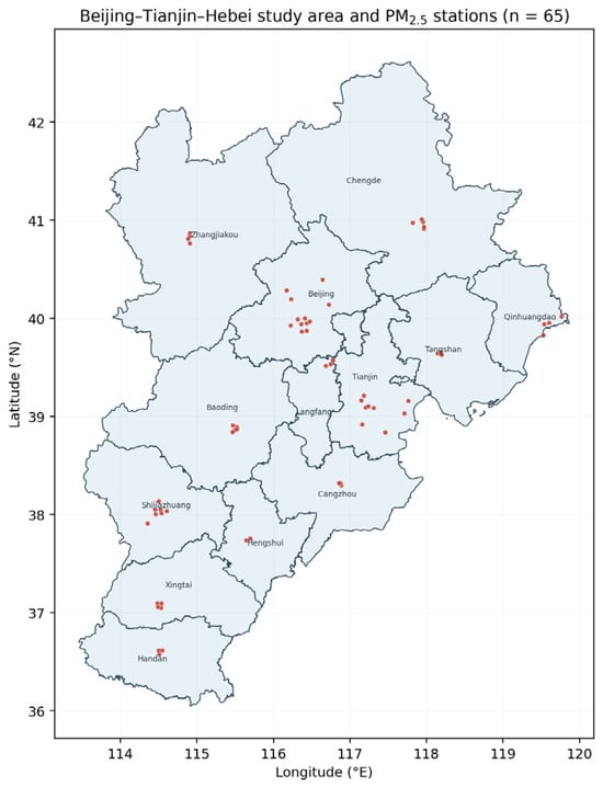
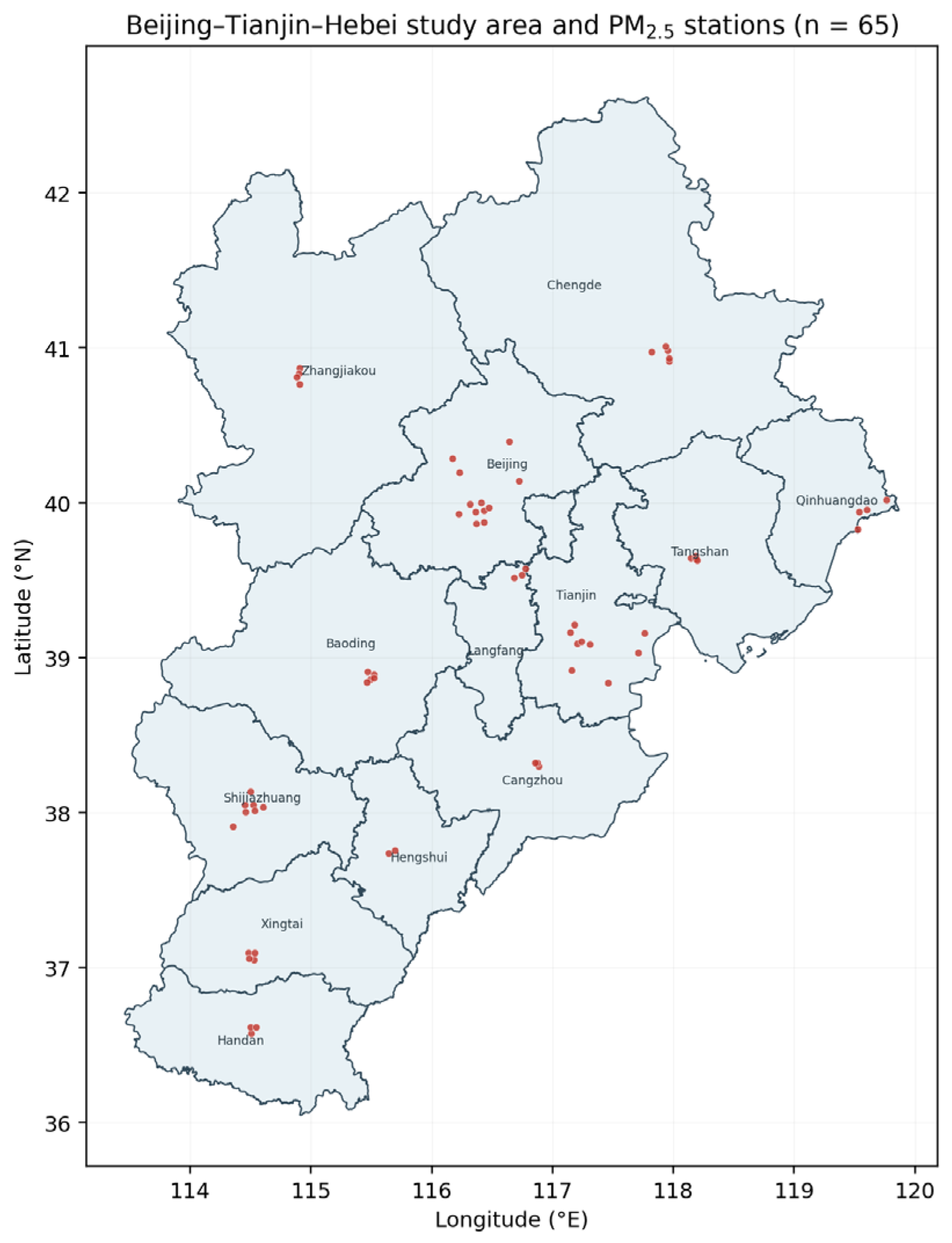
The target mapping region includes Beijing, Tianjin, and 11 prefecture-level cities in Hebei Province (BTH). It spans densely urbanized plains, industrial corridors, coastal areas, and mountainous northern and western terrain. After overpass-time correction and multispectral quality control, the model-development archive contained 12,768 satellite–meteorology collocations from 192 monitoring locations in 55 North China cities. Spatial restriction to the 13 BTH cities yielded 4210 collocations from 65 unique PM_2.5 stations and 96 WSI acquisition dates; these records were used for the strict date–station benchmark, while Figure 1 shows the BTH station network. PM_2.5 concentration was the regression target and is expressed in μg m⁻³.

Figure 1. Beijing–Tianjin–Hebei study area and the 65 unique PM_2.5 monitoring locations retained after spatial clipping and multispectral quality control.

2.2. DQ-1 WSI Data

The DQ-1 WSI provides a swath of approximately 2300 km and spatial resolutions ranging from 75 to 600 m, depending on channel and product [45]. The 2024 archive contained 100 GeoTIFF files. Ninety-eight unique date/scene-center combinations were identified; one four-band browse or auxiliary image was excluded, leaving 97 usable scene records. The source layers correspond nominally to 0.415, 0.443, 0.470, 0.490, 0.555, 0.659, 0.681, 0.753, approximately 0.8 (panchromatic), 0.865, 0.936, 0.940, 1.375, 1.640, and 2.130 μm [45]. The local rasters contained scaled integer signals rather than a consistently documented surface-reflectance product; they are therefore termed WSI band signals. B3 (0.470 μm) was retained for the final model only after controlled single-band and spectral-group comparison.

All WSI rasters were referenced to the China Geodetic Coordinate System 2000 (EPSG:4490) and stored nominal 12-bit signals. Pixels were retained only when all 15 bands were greater than 0 and less than 4095, B4 (0.490 μm) was below 2000, and the 1.375 μm cirrus-sensitive B13 signal was below 500. The combined rule rejects orbital-fill values, saturation, anomalously bright visible pixels, and elevated cirrus-like signals; because no validated per-pixel WSI cloud flag accompanied the GeoTIFFs, it is an empirical screening rule rather than a formal cloud mask. Inspection of available original metadata confirmed radiometric coefficient and solar/viewing-angle fields, but complete scene-specific coefficients and per-pixel geometry were not consistently available in the collocation archive. Consequently, no conversion to surface reflectance or angular normalization was claimed. The inversion grid was set to 0.02° to match the support of the multi-source analysis.

2.3. ERA5 Meteorological Data

ERA5 fields [47] were read from the local 2024 NetCDF archive on a 0.25° grid covering 30–45°N and 110–124°E. The variables were PBLH, 10 m zonal wind (u₁₀), 10 m meridional wind (v₁₀), and RH at 850 hPa. The archive contained 05:00 and 18:00 UTC fields. Acquisition time was evaluated from original DQ-1 H5 AssistData latitude/longitude footprints and DataSet/Time (seconds since 1 January 2000 12:00 UTC). Spatial nearest-footprint matching was available for 31 of the 96 WSI dates and yielded 04:45–05:38 UTC overpasses (median 05:22 UTC). A longitude–time relation fitted to those matches was used only to check the remaining scene centers; in every case 05:00 UTC was nearer than 18:00 UTC. All training and mapping meteorology was therefore extracted from 05:00 UTC and bilinearly interpolated to station or grid-cell coordinates. This is an archive-specific nearest-field assignment, not a general latitude rule; future archives with denser ERA5 times should use per-scene temporal interpolation.

2.4. CHAP Comparison Data

ChinaHighPM_2.5 is part of the China High Air Pollutants (CHAP) collection and provides seamless daily, monthly, and yearly ground-level PM_2.5 fields at 1 km resolution. The Version 4 monthly files for January–October and December 2024 were obtained from the official Zenodo record [54]. The files are expressed in μg m⁻³ and represent Beijing time calendar-month means. CHAP was used for product-level consistency assessment rather than independent validation or error-free ground truth, because it is itself a model-derived product informed by monitoring, satellite, meteorological, and auxiliary data [12,13,53,54]. The data sources and their roles are summarized in Table 1.

Table 1. Data sources and roles in the DQ-1 WSI PM_2.5 experiment.

Data	Variables	Nominal Support	Role
DQ-1 WSI	15 scaled band signals	75–600 m native; mapped at 0.02°	Selected spectral descriptor and optical–meteorological features
Ground monitoring	PM2.5	192 sites/12,768 North China records; 65 sites/4210 BTH records	Development target; strict BTH benchmark
ERA5	PBLH, u10, v10, RH at 850 hPa	0.25°; 05:00 UTC nearest to verified WSI overpasses	Mixing, humidity, and transport context
Administrative boundary	13 city polygons	Prefecture level	Masking, mapping, and city summaries

3. Methods

3.1. Quality Control and Collocation

Records were required to contain finite PM_2.5, date, city, station, coordinates, all 15 WSI signals, and the re-extracted 05:00 UTC ERA5 variables. The final multispectral quality-control rule required 0 < every band < 4095, B4 < 2000, and B13 < 500. The quality-control sensitivity analysis deliberately held the spectral input at B15 across all three filters, independently of the final B3 selection; the following values are fixed-fold out-of-fold scores, not repeated-fold means. The legacy B4 < 2500 filter retained 14,695 records and gave date-grouped R² = 0.3383 and RMSE = 35.21 μg m⁻³. Tightening B4 alone retained 13,031 records (R² = 0.3153; RMSE = 36.57 μg m⁻³), whereas adding the B13 cirrus-sensitive screen retained 12,768 records (R² = 0.3926; RMSE = 34.72 μg m⁻³). These controlled checks show that the result is sensitive to cloud/brightness screening; they do not establish universally transferable thresholds. All band trials used the final 12,768 collocations and identical folds. The strict BTH benchmark retained 4210 observations.

3.2. Physics-Guided Feature Engineering

The original baseline predictor set contained the 15 WSI signals, WSI-pixel and station coordinates, PBLH, u₁₀, v₁₀, and RH. For mapping, station coordinates were set equal to grid-cell coordinates because the training station and matched WSI-pixel coordinates differed only by the collocation offset. The selected-band model used B3 together with the same contextual variables and transformations motivated by aerosol hygroscopicity, boundary-layer dilution, and ventilation. These transformations guide feature construction but do not impose physical constraints on ExtraTrees (Table 2).

Table 2. Predictor groups used by the original-feature baseline and physics-guided ExtraTrees models.

Predictor Group	Representative Variables	Baseline	Physics-Guided
WSI spectral	Bands 1–15/selected B3	All 15	B3
Spatial	Pixel/station longitude and latitude	Yes	Yes
Meteorological	PBLH, u10, v10, RH	Yes	Yes
Signal summaries	Selected-input mean, median, anchor	No	Yes
RH–PBLH interactions	fRH, Lmean, Lmedian, fRH/PBLH	No	Yes
Transport	Wind speed and normalized components	No	Yes
Calendar	Month and day-of-year sine/cosine	No	Yes

A hygroscopic growth proxy was defined as fRH = [max(1 − RH/100, 0.05)]^−0.30. PBLH was converted to kilometers, and optical–meteorological indices were formed as L_mean = S_mean × fRH/(PBLH_km + 0.10) and L_median = S_median × fRH/(PBLH_km + 0.10), where S_mean and S_median are scaled signal summaries of the tested spectral input. The 0.10 km term prevents numerical instability under shallow boundary layers. Wind speed, normalized zonal and meridional components, fRH/(PBLH_km + 0.10), and sine/cosine encodings of month and day of year were also included. These are heuristic, physics-guided predictors rather than retrieved AOD, aerosol mass, or a physically constrained forward model; definitions are summarized in Table S1.

3.3. ExtraTrees Modeling and Model Selection

ExtraTrees averages randomized regression trees [48]. The full contextual mapping configuration used B3, meteorology, physics-guided transformations, coordinates, calendar encodings, 180 trees for validation, min_samples_leaf = 2, and 500 trees for final scene inversion. To separate model components, the controlled staged ablation fixed 180 trees, min_samples_leaf = 2, random seeds, samples, and folds while sequentially testing: 15 bands plus meteorology; B3 plus meteorology; physics-guided terms; coordinates; and calendar encodings. A second full contextual run with min_samples_leaf = 1 isolated the leaf-size effect. Exploratory band screening used 120 trees, and the ExtraTrees, XGBoost, and LightGBM settings for the strict benchmark are listed in Table S2.

3.4. WSI Band Screening and Selection Rule

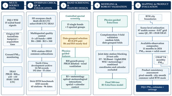
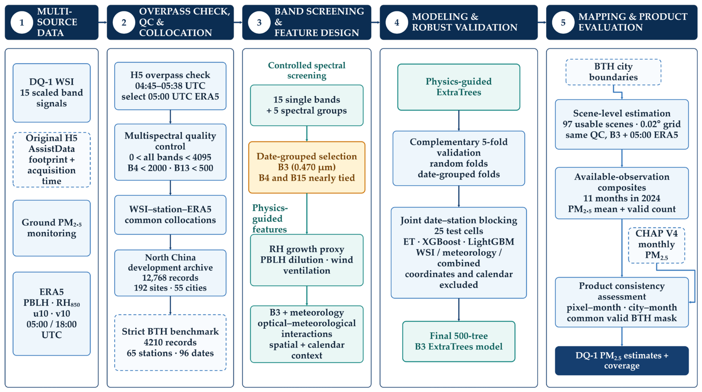
Band screening separated the tested WSI spectrum from the shared meteorological and spatiotemporal predictors. Fifteen single-band models were fitted, each containing one WSI channel plus the same coordinate, ERA5, RH–PBLH, wind, and cyclic-date features. Five spectral-group models were then fitted: B1–B4 (blue), B1–B8 (visible/red-edge), B1–B12 (visible–near infrared), B1–B8 plus B13–B15 (visible–shortwave infrared), and B1–B15 (full WSI). All comparisons used the same 12,768 quality-controlled records, model family, and folds (Figure 2). Selection was based on maximum date-grouped five-fold R², with lower RMSE as the tie-breaker, because the intended application requires transfer to unseen acquisition dates.

Figure 2. Workflow for H5-informed overpass checking, DQ-1 WSI multispectral quality control, pre-specified band screening, physics-guided feature construction, strict transfer assessment, and contextual multi-month PM_2.5 mapping.

The single-band and multi-band experiments answer different questions. The fixed GroupKFold allocation was retained as the pre-specified selection analysis. Ranking uncertainty was assessed separately by ten balanced reallocations of the 96 acquisition dates to five folds; each repetition used the same samples, fold assignments, predictors, and model settings for all 15 bands. We report the mean and standard deviation of R² and RMSE, the number of first-place rankings, and paired percentile intervals for B3 relative to B4 and B15. This sensitivity analysis was not used to reselect a channel after inspecting the outcomes.

3.5. Validation Design

Two complementary five-fold schemes were used. Random five-fold validation shuffled individual records and measured interpolation among the sampled spatiotemporal conditions. Date-grouped five-fold validation kept all records from the same WSI acquisition date in one fold, preventing date leakage and testing transfer to unseen dates. Model performance was summarized by the coefficient of determination (R²), root mean square error (RMSE), mean absolute error (MAE), mean bias, and mean residual for observations above 200 μg m⁻³. The same fold assignments were used for baseline and enhanced models [50].

3.6. Joint Spatiotemporal Blocking and Unified Benchmark

The strict benchmark used 4210 collocations from the 13 BTH cities, comprising 65 stations and 96 WSI acquisition dates. Dates and stations were independently assigned to five GroupKFold blocks. The 25 date-block × station-block intersections served as test cells; for each cell, training excluded every record belonging either to the held-out date block or to the held-out station block. Training sets contained 2672–2729 records (median 2690), and test cells contained 158–179 records (median 169). Thus, neither a test date nor a test station appeared in training, and every BTH record received one out-of-fold prediction. This cross-classified design evaluates simultaneous temporal and spatial transfer rather than interpolation at previously observed stations.

ExtraTrees, XGBoost, and LightGBM were compared using the same 4210 samples and folds [57,58]. Three strictly separated configurations were evaluated: WSI only (B3), meteorology only (PBLH, RH, u₁₀, v₁₀, wind magnitude/direction, and RH–PBLH transformations), and WSI + meteorology (their union plus B3–RH–PBLH and B3–wind interactions). Coordinates and calendar variables were omitted so that spectral and meteorological contributions were not conflated with explicit location or seasonal identifiers. Hyperparameters were fixed before comparison (Table S2); the benchmark is a controlled robustness analysis, not exhaustive tuning.

3.7. Scene Inversion and Compositing

Each unique WSI scene was reprojected to the fixed BTH grid. The same 15-band range, B4 brightness, and B13 cirrus-sensitive screens used for training were applied to every grid cell; B3 supplied the pre-specified spectral descriptor. Corrected 05:00 UTC ERA5 fields were interpolated and passed through the 500-tree full contextual model together with physics-guided terms, grid-cell coordinates, and known scene-date encodings. This configuration was retained to describe within-2024 spatial and seasonal patterns because those contextual variables are available for every mapped cell and scene. It is distinct from the coordinate- and calendar-free strict benchmark, which governs claims about transfer and incremental WSI information. Predictions were constrained to 0–500 μg m⁻³ and averaged by month and across available scenes. The maps are therefore contextual available-observation composites, not evidence of coordinate- and calendar-free predictive skill or regulatory exposure surfaces.

3.8. Comparison with CHAP

For each month with a DQ-1 composite, the corresponding CHAP M1K field was sampled to the centers of the 0.02° DQ-1 grid by nearest-neighbor assignment and clipped to the common valid BTH mask. Monthly spatial Pearson correlation, identity-line R², RMSE, MAE, and mean difference (DQ-1 minus CHAP) were computed from the common grid cells. A pooled pixel–month comparison combined all 11 matched months. To reduce the influence of spatial autocorrelation and resolution mismatch, a second comparison averaged both datasets within each of the 13 city polygons for every available month, producing 143 city–month pairs. Because DQ-1 composites average only valid satellite scenes whereas CHAP represents complete calendar-month means, these diagnostics measure consistency between products rather than formal validation of either product.

4. Results

4.1. DQ-1 WSI Band Screening and Ranking Stability

Under the pre-specified date-grouped five-fold allocation, B3 (0.470 μm) ranked first (R² = 0.3952; RMSE = 34.64 μg m⁻³), followed closely by B4 (R² = 0.3941) and B15 (R² = 0.3926). The ten repeated balanced date-block allocations changed this ordering: mean R² was 0.3506 ± 0.0274 for B14, 0.3461 ± 0.0299 for B15, 0.3373 ± 0.0311 for B3, and 0.3316 ± 0.0255 for B4; no channel ranked first more than twice. The paired B3−B4 R² interval was −0.0126 to 0.0259, and the B3−B15 interval was −0.0318 to 0.0080. Both include zero. B3 is therefore retained as the channel selected by the pre-specified split, not as a statistically distinct or universally optimal WSI band (Table 3).

Table 3. Fixed and repeated date-grouped validation of all 15 DQ-1 WSI bands. Fixed metrics use the pre-specified GroupKFold allocation; repeated metrics summarize ten balanced date-block allocations. First rank is the number of repetitions in which a band ranked first.

Band	Wavelength (μm)	Fixed R2	Fixed RMSE	Repeated R2 Mean	Repeated R2 SD	Repeated RMSE	First Rank/10
B1	0.415	0.3790	35.11	0.3397	0.0269	36.19	2
B2	0.443	0.3709	35.34	0.3411	0.0266	36.16	0
B3	0.470	0.3952	34.64	0.3373	0.0311	36.26	0
B4	0.490	0.3941	34.68	0.3316	0.0255	36.42	0
B5	0.555	0.3826	35.00	0.3427	0.0272	36.11	0
B6	0.659	0.3919	34.74	0.3426	0.0300	36.11	0
B7	0.681	0.3902	34.79	0.3404	0.0278	36.17	0
B8	0.753	0.3828	35.00	0.3416	0.0248	36.14	0
B9	~0.800 pan	0.3874	34.87	0.3490	0.0295	35.94	2
B10	0.865	0.3898	34.80	0.3467	0.0291	36.00	1
B11	0.936	0.3743	35.24	0.3439	0.0341	36.07	2
B12	0.940	0.3855	34.92	0.3470	0.0282	35.99	0
B13	1.375	0.3886	34.83	0.3489	0.0220	35.94	1
B14	1.640	0.3912	34.76	0.3506	0.0274	35.89	1
B15	2.130	0.3926	34.72	0.3461	0.0299	36.01	1

Among the five multi-band configurations, B1–B4 produced the highest score in the pre-specified date allocation (R² = 0.3919; RMSE = 34.74 μg m⁻³), followed by B1–B8 (R² = 0.3839) and B1–B12 (R² = 0.3822). B3 alone slightly exceeded the best group under that fixed rule and was retained under the pre-specified mapping protocol rather than being reselected from the sensitivity analysis. The repeated analysis shows that this operational choice is fold-sensitive; it does not show that B3 is spectrally superior (Table 4).

Table 4. Controlled DQ-1 WSI spectral-group comparison after overpass-time correction and multispectral quality control. Rank is determined by date-grouped five-fold validation.

Spectral Configuration	Bands	Random R2	Random RMSE	Date R2	Date RMSE	Rank
B1–B4: blue	4	0.9272	12.02	0.3919	34.74	1
B1–B8: visible/red-edge	8	0.9256	12.15	0.3839	34.97	2
B1–B12: visible–NIR	12	0.9272	12.02	0.3822	35.02	3
B1–B8 + B13–B15: visible–SWIR	11	0.9254	12.17	0.3763	35.18	4
B1–B15: full WSI	15	0.9262	12.10	0.3587	35.67	5

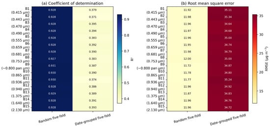
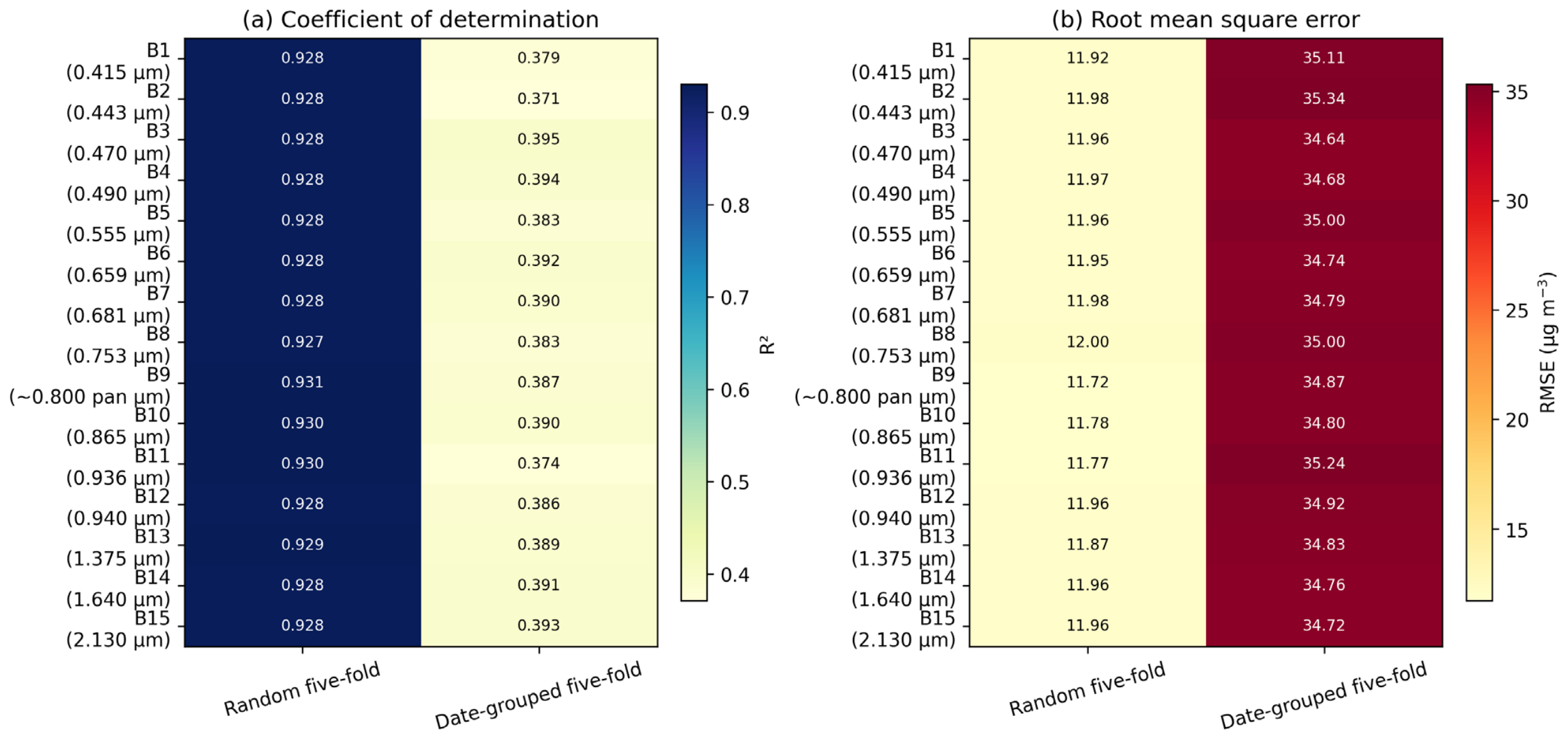
Random-fold performance was tightly clustered (R² = 0.9275–0.9308), whereas the pre-specified date-grouped R² ranged from 0.3709 to 0.3952. Repeated date-block allocation produced mean R² values from 0.3316 to 0.3506 and distributed first-place rankings across several channels. The ordering is therefore sensitive both to validation design and to the particular date partition. Figure 3 reports the fixed-fold pattern, while Table 3 reports the repeated-fold uncertainty.

Figure 3. Heatmaps of (a) R² and (b) RMSE (μg m⁻³) for all 15 DQ-1 WSI channels under random and date-grouped five-fold validation. B3 ranked first under the date-grouped rule; B4 and B15 were closely comparable.

The B3 result is physically plausible because blue-channel signals respond to aerosol scattering, but it is not uniquely attributable to aerosol. B3 correlated strongly with the neighboring B4 signal (r = 0.987) and only weakly with PM_2.5 (r = −0.031), PBLH (r = 0.020), and RH (r = 0.138). It should therefore be interpreted as a predictive scene descriptor containing mixed atmospheric, surface, residual-cloud, calibration, and geometry information. Likewise, the near-top B15 performance may partly reflect reduced sensitivity to some visible-surface and cloud effects rather than direct PM_2.5 sensitivity. Independent radiative-transfer and calibrated-reflectance analyses are required for causal attribution.

4.2. Controlled Attribution of Model Components

A direct baseline-to-full-model contrast changes the spectral input, engineered features, calendar variables, and leaf size simultaneously and therefore cannot isolate any one component. In the controlled date-grouped ablation with identical 180-tree models and min_samples_leaf = 2, 15 bands plus meteorology yielded R² = 0.2737 and RMSE = 37.97 μg m⁻³. Replacing the 15 bands with B3 reduced R² to 0.1519; adding physics-guided terms gave R² = 0.1516; adding coordinates gave R² = 0.1640; and adding calendar encodings raised R² to 0.3919 and reduced RMSE to 34.74 μg m⁻³ (Table 5). Thus, the full contextual score cannot be attributed to band reduction or physical feature construction alone.

Table 5. Controlled date-grouped staged ablation. All main stages used the same 12,768 records, folds, random seeds, 180 trees, and min_samples_leaf = 2; the leaf = 1 row isolates the hyperparameter effect.

Stage	Configuration	Leaf	R2	RMSE	MAE	Change Isolated
A1	15 bands + met.	2	0.2737	37.97	24.20	Starting point
A2	B3 + met.	2	0.1519	41.03	27.13	Band reduction
A3	B3 + met. + physics	2	0.1516	41.03	27.26	Physics terms
A4	B3 + met. + physics + coordinates	2	0.1640	40.73	26.47	Coordinates
A5	B3 + met. + physics + coordinates + calendar	2	0.3919	34.74	21.76	Calendar
H1	Full contextual configuration; leaf = 1	1	0.3788	35.11	21.90	Leaf size
C1	15-band raw contextual comparator	2	0.2421	38.78	24.58	Contextual reference

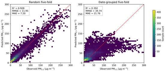
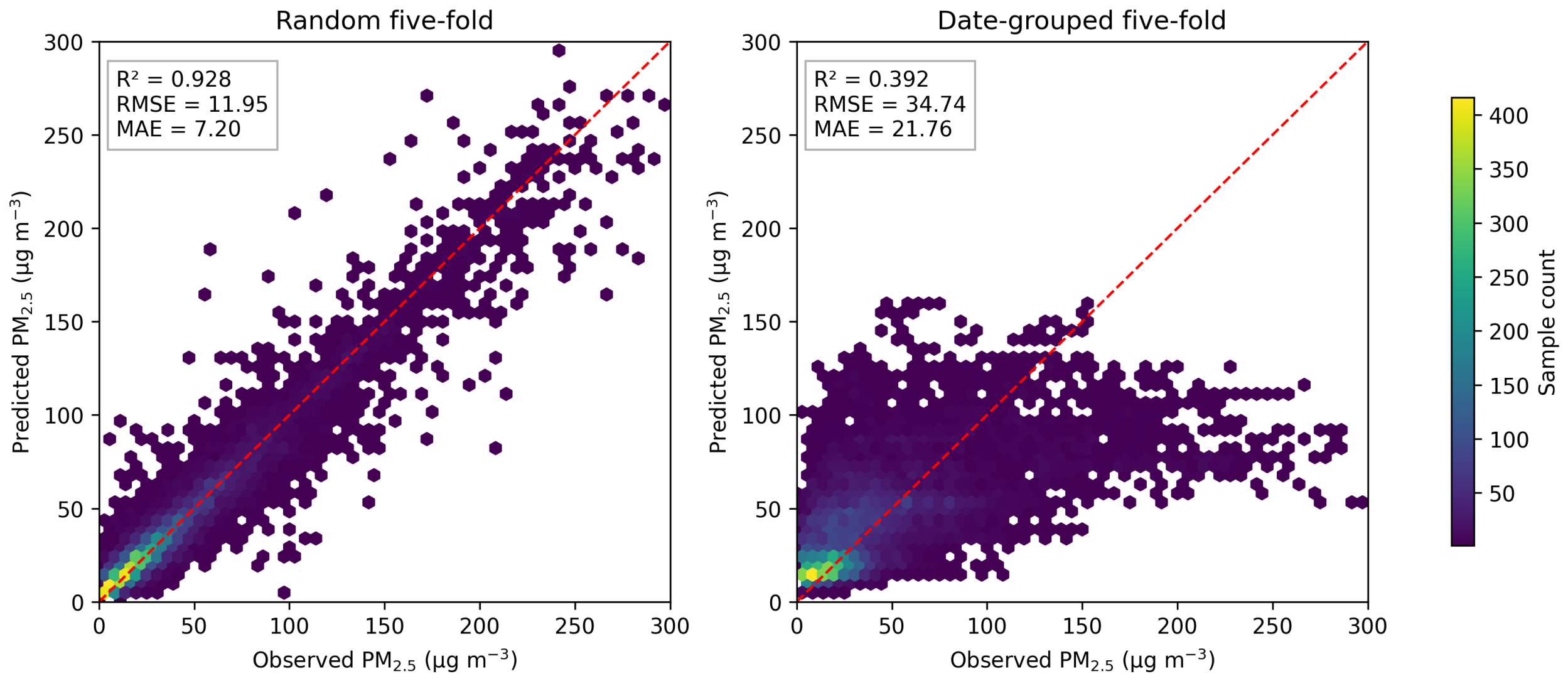
The separate leaf-size sensitivity changed the full contextual date-grouped R² from 0.3919 at min_samples_leaf = 2 to 0.3788 at min_samples_leaf = 1, with RMSE increasing from 34.74 to 35.11 μg m⁻³. Under random validation, the full contextual configuration achieved R² = 0.9280 and RMSE = 11.95 μg m⁻³, but this interpolation score is not used as evidence of transfer. More importantly, date-grouped bias above 200 μg m⁻³ was −158.27 μg m⁻³. The model therefore does not reconstruct severe-event peaks, regardless of its performance for the dominant concentration range (Figure 4 and Table 6).

Figure 4. Observed versus out-of-fold predicted PM_2.5 for the selected-B3 ExtraTrees model under random five-fold (left) and date-grouped five-fold (right) validation. Units are μg m⁻³.

Table 6. Error of the selected-B3 model stratified by observed PM_2.5 concentration. Bias is prediction minus observation; RMSE, MAE, and bias are in μg m⁻³.

Observed Class	Validation	n	RMSE	MAE	Bias
≤35	Random five-fold	7826	7.49	5.20	2.24
≤35	Date-grouped five-fold	7826	21.19	14.97	11.85
>35–75	Random five-fold	3038	11.17	7.85	−0.89
>35–75	Date-grouped five-fold	3038	23.39	17.70	0.32
>75–115	Random five-fold	1001	18.28	12.85	−4.35
>75–115	Date-grouped five-fold	1001	35.98	30.84	−25.03
>115–150	Random five-fold	411	17.57	10.95	−5.36
>115–150	Date-grouped five-fold	411	53.22	47.21	−44.86
>150–200	Random five-fold	287	21.46	14.46	−5.41
>150–200	Date-grouped five-fold	287	87.77	84.17	−83.94
>200	Random five-fold	205	44.85	28.41	−21.93
>200	Date-grouped five-fold	205	164.71	158.27	−158.27

The date-grouped error increased monotonically with concentration. The ≤35 μg m⁻³ class had RMSE = 21.19 μg m⁻³ and bias = 11.85 μg m⁻³; bias became negative above 75 μg m⁻³, reached −83.94 μg m⁻³ at 150–200 μg m⁻³, and was −158.27 μg m⁻³ above 200 μg m⁻³. Only 205 of 12,768 records (1.61%) exceeded 200 μg m⁻³, and 91.2% of those cases occurred when PBLH was ≤1000 m. The error pattern is consistent with response imbalance, regression toward the dominant range, shallow-layer episode structure, and possible spectral saturation or out-of-distribution conditions. The model is therefore suitable for regional pattern analysis but not for estimating severe-event peaks (Table 6).

4.3. Unified Algorithm, Feature-Ablation, and Joint-Block Results

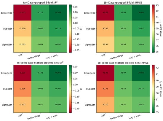
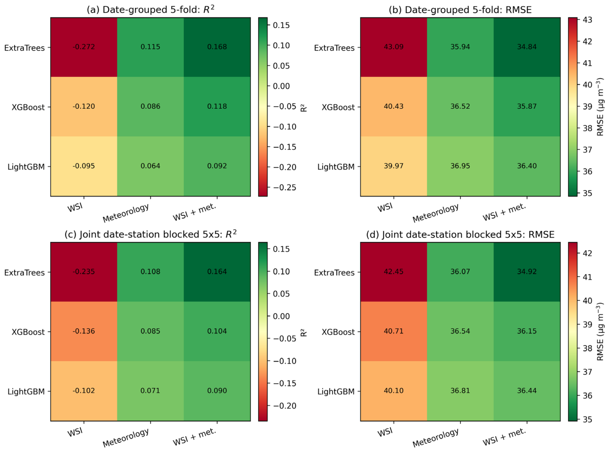
The corrected BTH benchmark retained the same hierarchy across both transfer tests (Table 7 and Figure 5). Under date grouping, WSI + meteorology achieved R² values of 0.1681, 0.1180, and 0.0920 for ExtraTrees, XGBoost, and LightGBM, with RMSE values of 34.84, 35.87, and 36.40 μg m⁻³. Under joint date–station blocking, the corresponding R² values were 0.1643, 0.1045, and 0.0901. ExtraTrees was the strongest algorithm under the fixed settings, but its joint-block R² remained modest, delimiting simultaneous temporal and station transfer.

Table 7. Unified comparison of algorithms and strictly separated feature configurations on 4210 BTH collocations. Joint blocking excludes both the test-date block and test-station block from training.

Algorithm	Features	Validation	R2	RMSE	MAE
ExtraTrees	WSI only	Date	−0.2725	43.09	30.79
ExtraTrees	WSI only	Date + station	−0.2349	42.45	30.32
ExtraTrees	Meteorology only	Date	0.1145	35.94	25.28
ExtraTrees	Meteorology only	Date + station	0.1085	36.07	25.38
ExtraTrees	WSI + meteorology	Date	0.1681	34.84	24.63
ExtraTrees	WSI + meteorology	Date + station	0.1643	34.92	24.68
XGBoost	WSI only	Date	−0.1204	40.43	28.98
XGBoost	WSI only	Date + station	−0.1356	40.71	29.17
XGBoost	Meteorology only	Date	0.0861	36.52	25.38
XGBoost	Meteorology only	Date + station	0.0852	36.54	25.53
XGBoost	WSI + meteorology	Date	0.1180	35.87	25.06
XGBoost	WSI + meteorology	Date + station	0.1045	36.15	25.37
LightGBM	WSI only	Date	−0.0951	39.97	28.72
LightGBM	WSI only	Date + station	−0.1022	40.10	28.80
LightGBM	Meteorology only	Date	0.0642	36.95	25.86
LightGBM	Meteorology only	Date + station	0.0714	36.81	25.76
LightGBM	WSI + meteorology	Date	0.0920	36.40	25.59
LightGBM	WSI + meteorology	Date + station	0.0901	36.44	25.52

Figure 5. Unified comparison of ExtraTrees, XGBoost, and LightGBM using WSI-only, meteorology-only, and WSI–meteorology predictors under date-grouped and joint date–station blocked validation. Coordinates and calendar variables were excluded from this strict ablation experiment.

WSI-only models did not generalize under joint blocking (R² = −0.2349, −0.1356, and −0.1022 for ExtraTrees, XGBoost, and LightGBM). Meteorology-only R² values were 0.1085, 0.0852, and 0.0714; combining WSI and meteorology increased them to 0.1643, 0.1045, and 0.0901. For ExtraTrees, adding B3 and its interaction terms reduced joint-block RMSE from 36.07 to 34.92 μg m⁻³ (3.18%). Thus, this is primarily a meteorology-dominated estimation problem with an incremental, conditional WSI contribution rather than an independently skillful WSI retrieval.

4.4. Predictor Importance

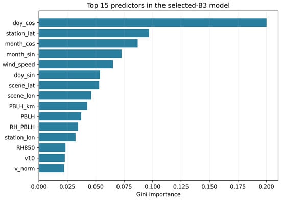
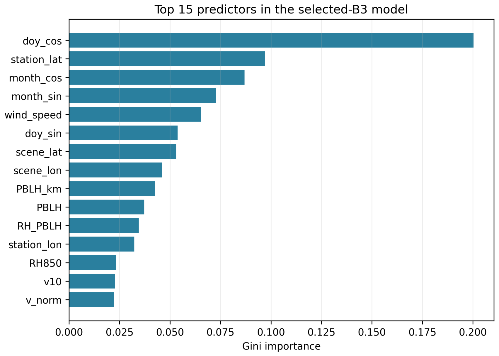
Day-of-year cosine was the most influential predictor in the full contextual mapping model (Gini importance = 0.200), followed by station latitude (0.097), month cosine (0.087), and month sine (0.073) (Figure 6). The staged ablation confirms this dependence: the coordinate-free, calendar-free B3–meteorology–physics model gave date-grouped R² = 0.1516; coordinates increased it only to 0.1640, whereas calendar encodings increased it to 0.3919. By contrast, the strict BTH joint-block benchmark excluded both coordinates and calendar variables and yielded R² = 0.1643 for ExtraTrees with WSI plus meteorology. These results measure different tasks. The full model describes spatial and seasonal covariance within the sampled 2024 archive; the strict benchmark measures simultaneous transfer to withheld date and station blocks and is the basis for claims about incremental WSI information. Feature importance is predictive, not causal.

Figure 6. Gini importance of the 15 highest-ranked predictors in the selected-B3 ExtraTrees model with physics-guided feature engineering.

4.5. B3 PM_2.5 Estimation and Retrieval Coverage

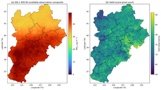
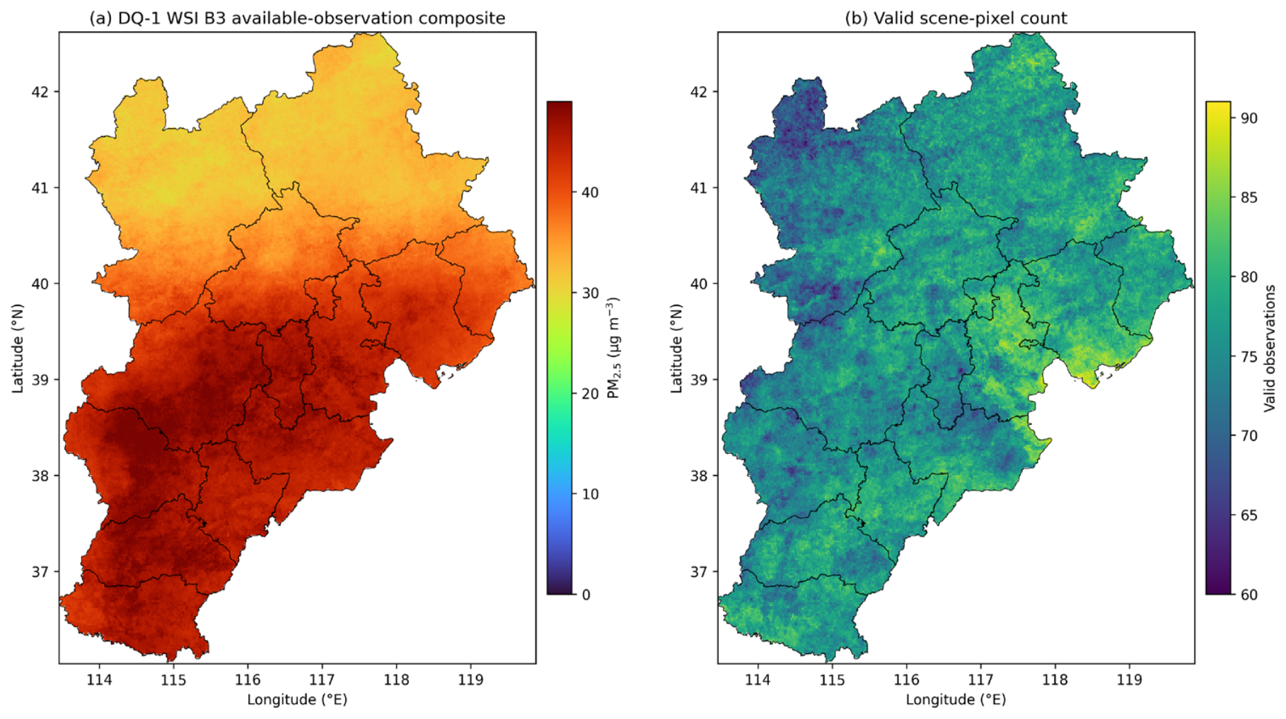
Ninety-seven usable scene records contributed valid estimates. Across the fixed BTH grid, 56,916 cells had at least one estimate; the median and mean valid counts were 77.0 and 76.44, and the maximum was 91. The available-observation composite showed higher predicted concentrations over the southern and central plain and lower values over northern mountainous cities. The multispectral screening reduced the per-cell count relative to the original implementation, and Figure 7 therefore reports concentration together with valid-observation coverage. The composite is an observation-weighted product, not a regulatory annual mean.

Figure 7. (a) Selected-B3 available-observation PM_2.5 composite for 2024 and (b) number of valid scene-pixel estimates contributing to each grid cell. The concentration composite is not a gap-free annual mean.

4.6. Multi-Month Spatial Results

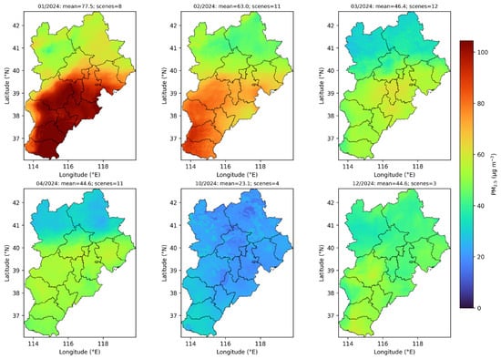
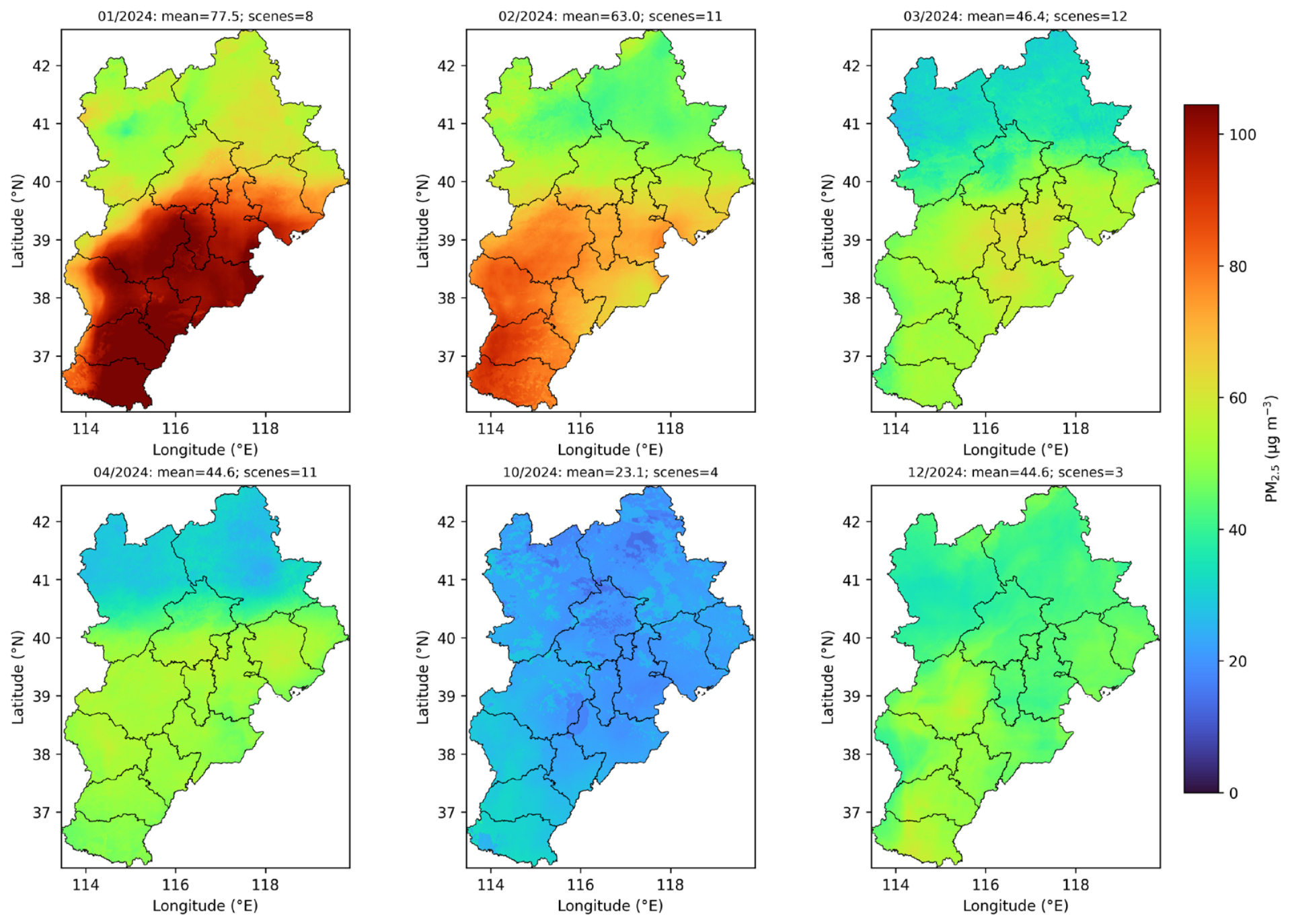
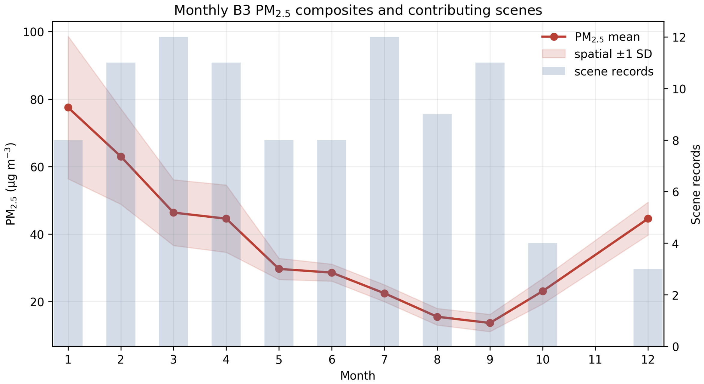
The B3 monthly composites provide valid regional coverage in January–October and December; November had no source scene. Mean PM_2.5 was 77.52 μg m⁻³ in January, 63.02 in February, 46.38 in March, and 44.58 in April. The May–July means were 29.70, 28.61, and 22.48 μg m⁻³; August and September were 15.53 and 13.68 μg m⁻³. October and December means were 23.10 and 44.60 μg m⁻³. Figure 8 shows six representative months. These values summarize only valid acquisition scenes and should not be interpreted as complete calendar-month exposure means.

Figure 8. Spatial distributions from the selected-B3 model for January, February, March, April, October, and December 2024. Titles report regional available-observation mean PM_2.5 (μg m⁻³) and contributing scene count.

The source archive was temporally uneven. March and July each contained 12 scene records; February, April, and September contained 11; and October and December contained four and three. Monthly covered cells ranged from 56,105 to 56,916, but similar spatial support does not imply equal temporal representativeness. Table 8 and Figure 9 therefore summarize acquisition-conditioned products rather than climatological monthly means.

Table 8. Monthly available-observation statistics from the selected-B3 model.

Month	Mean PM2.5	Spatial SD	Covered Pixels	Scene Records
1	77.52	21.13	56,916	8
2	63.02	14.17	56,916	11
3	46.38	9.75	56,916	12
4	44.58	9.97	56,916	11
5	29.70	3.14	56,914	8
6	28.61	2.52	56,105	8
7	22.48	2.50	56,916	12
8	15.53	2.47	56,914	9
9	13.68	2.56	56,916	11
10	23.10	3.77	56,916	4
12	44.60	4.87	56,916	3

Figure 9. Monthly selected-B3 available-observation PM_2.5 means, spatial standard deviations, and contributing scene records. November is blank because no WSI scene was supplied.

Spatial standard deviation was highest in January (21.13 μg m⁻³), followed by February (14.17), April (9.97), and March (9.75 μg m⁻³). It was 2.47–3.14 μg m⁻³ from May to September and increased to 3.77 and 4.87 μg m⁻³ in October and December. These contrasts describe the available scenes; the low number of autumn and winter acquisitions limits seasonal inference.

4.7. Product-Level Comparison with CHAP

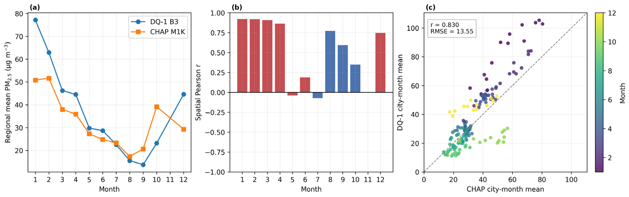
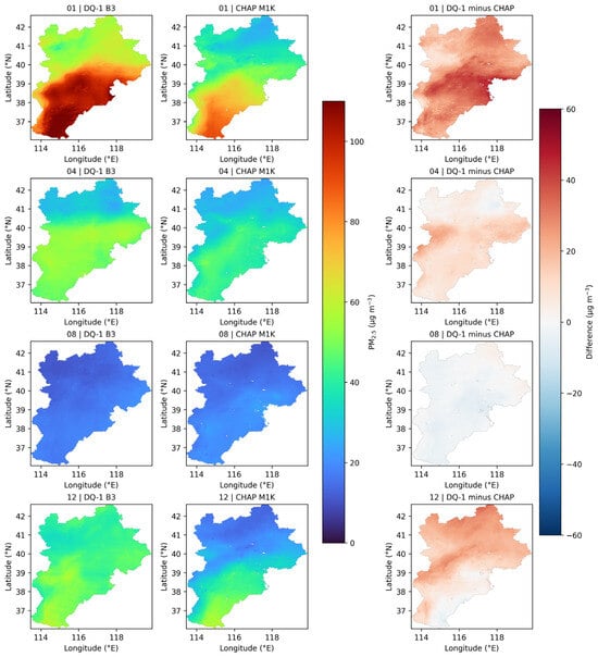
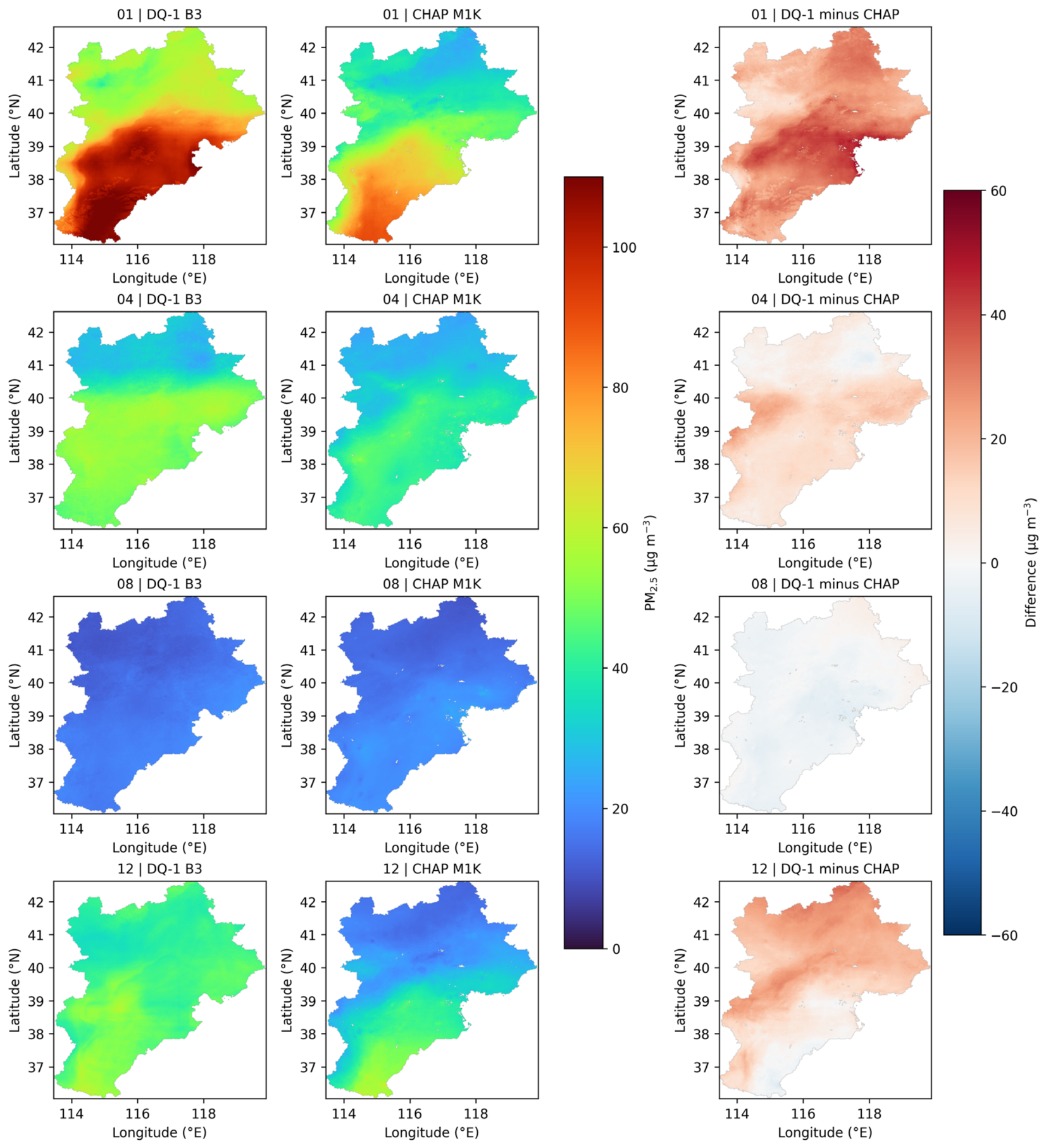
Across 614,965 common pixel–month pairs, DQ-1 and CHAP had Pearson r = 0.799, identity-line R² = 0.169, RMSE = 13.68 μg m⁻³, MAE = 10.10 μg m⁻³, and mean difference = 4.61 μg m⁻³. At the city–month scale (n = 143), r = 0.830, RMSE = 13.55 μg m⁻³, MAE = 10.16 μg m⁻³, and mean difference = 3.44 μg m⁻³. These statistics indicate shared broad variability but material magnitude differences; they are product-consistency measures, not independent validation.

Spatial agreement was strongest in January (r = 0.922), February (0.918), and March (0.906), while May and July were near zero (−0.040 and −0.073). DQ-1 exceeded CHAP by 26.38 μg m⁻³ in January and 15.31 μg m⁻³ in December; the largest negative difference occurred in October (−16.01 μg m⁻³), when only four WSI scenes contributed. Table 9 and Figure 10 and Figure 11 show that agreement depends strongly on season and within-month sampling.

Table 9. Monthly common-grid comparison between DQ-1 B3 available-observation composites and CHAP M1K calendar-month means.

Month	DQ-1 Mean	CHAP Mean	Pearson r	RMSE	MAE	Difference
1	77.20	50.82	0.922	27.69	26.38	26.38
2	62.89	51.64	0.918	12.72	11.28	11.25
3	46.23	37.95	0.906	9.30	8.32	8.28
4	44.51	35.87	0.862	10.20	8.77	8.63
5	29.76	27.28	−0.040	5.99	4.96	2.48
6	28.62	24.73	0.188	6.07	5.06	3.90
7	22.48	23.25	−0.073	5.53	4.83	−0.77
8	15.47	17.29	0.772	2.74	2.32	−1.82
9	13.70	20.63	0.593	8.27	7.02	−6.93
10	23.14	39.15	0.350	21.16	16.58	−16.01
12	44.59	29.28	0.747	17.63	15.51	15.31

Figure 10. DQ-1–CHAP product comparison: (a) regional monthly means, (b) monthly spatial Pearson correlation, and (c) city–month means for 13 cities and 11 matched months. CHAP is not treated as independent ground truth.

Figure 11. Spatial comparison for January, April, August, and December 2024. Columns show the DQ-1 B3 composite, CHAP M1K field sampled to the DQ-1 grid, and DQ-1 minus CHAP. CHAP is displayed only within the valid DQ-1 mask.

5. Discussion

5.1. Interpretation of the Band-Selection Result

B3 ranked first under the pre-specified date allocation, but the repeated analysis did not identify a stable single-band winner. Across ten balanced date-block reallocations, B14 had the highest mean R², no band ranked first more than twice, and the paired B3 differences relative to B4 and B15 both had intervals spanning zero. B3 was retained to preserve the pre-specified mapping pipeline rather than reselecting a channel after seeing the sensitivity results. Its role is therefore an archive- and split-conditional scene descriptor, not evidence that 0.470 μm is universally optimal or that B3 directly measures PM_2.5.

The controlled staged ablation constrains the interpretation of the full-model result. Replacing 15 bands with B3 did not improve date-blocked transfer, and physics-guided terms alone produced almost no change; the large increase to R² = 0.3919 occurred after calendar encodings were introduced. The leaf-size effect was comparatively small. Accordingly, the aggregate RMSE/MAE difference cannot be interpreted as evidence for a single methodological component. The strict coordinate- and calendar-free benchmark, rather than the full contextual model, is used to quantify the conditional WSI contribution.

5.2. Physical Interpretation

RH, PBLH, and wind are physically relevant context, but the constructed terms are heuristic. Date-blocked RMSE was 57.16 μg m⁻³ for PBLH ≤ 500 m, compared with 20.80 μg m⁻³ above 1500 m; the shallowest-PBLH stratum also had bias = −21.78 μg m⁻³. Moreover, 91.2% of observations above 200 μg m⁻³ occurred at PBLH ≤ 1000 m. This concentration of severe events under shallow mixing, combined with their 1.61% sample frequency, helps explain the large negative extreme-event bias. It does not establish a causal PBLH error mechanism because episode emissions, RH, spectral response, and synoptic transport covary. The optical–meteorological terms should therefore be interpreted as physics-guided features, not retrieved AOD or a mechanistic aerosol model.

The strict ablation further constrains interpretation. Meteorology-only models retained limited positive skill, whereas B3-only models did not outperform a mean predictor. Adding B3 and its atmosphere-interaction terms improved all three algorithms relative to meteorology alone, but the gains were modest. The full contextual configuration used for Figure 7, Figure 8, Figure 9, Figure 10, Figure 11, Figure 12 and Figure 13 additionally includes coordinates and calendar encodings because the mapping objective is to summarize the sampled 2024 archive at known grid cells and dates. Those maps are therefore explicitly labeled contextual available-observation composites. They are not presented as estimates from the strict transfer model, and the lower coordinate- and calendar-free blocked scores govern any claim about generalization.

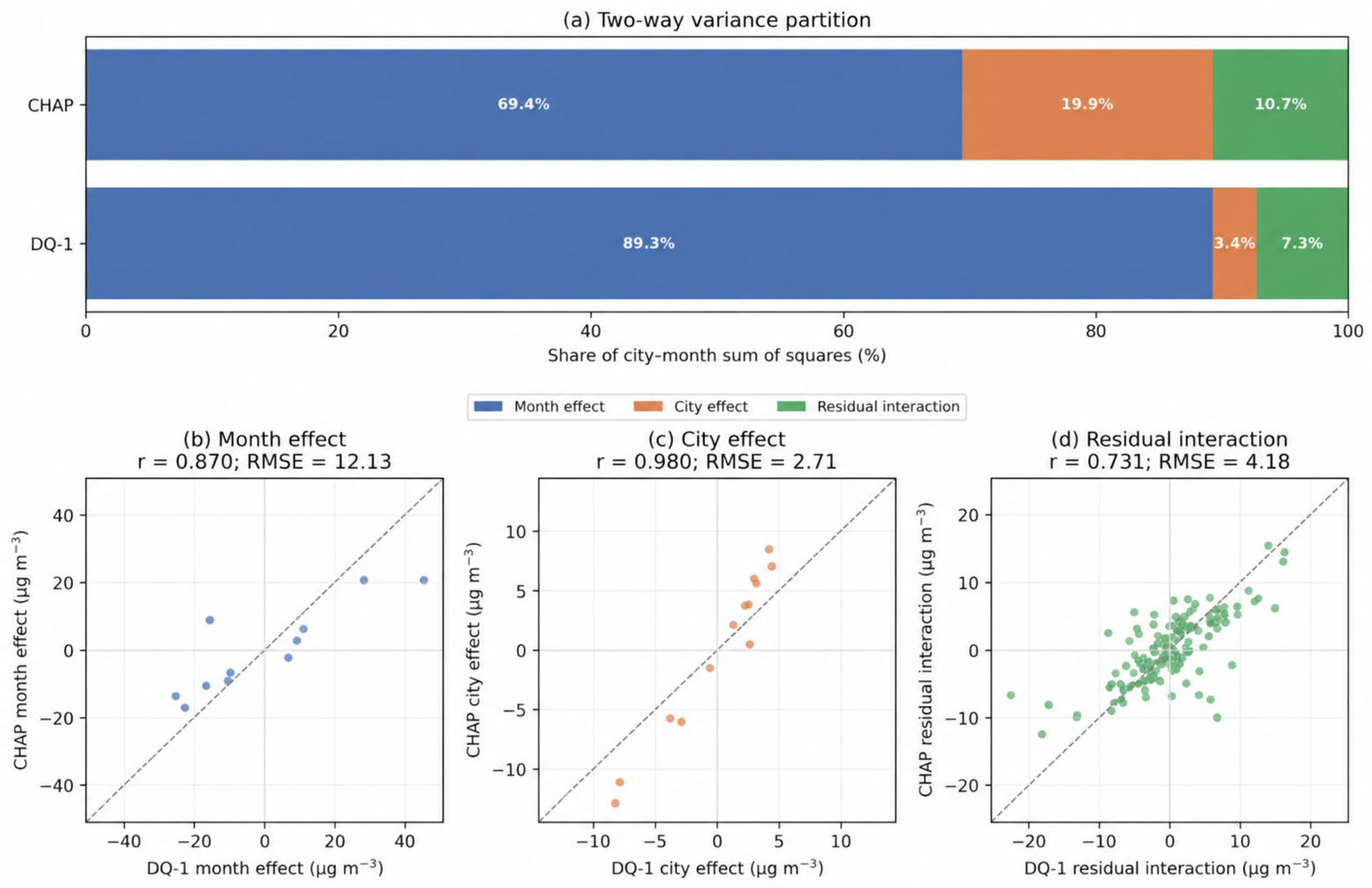
Figure 12. Two-way decomposition of the 143 DQ-1–CHAP city–month pairs. (a) Shares of total city–month sum of squares attributed to month, city, and residual city–month interaction effects. Panels (b–d) compare corresponding DQ-1 and CHAP effects after centering. The residual interaction comparison removes both overall seasonal and persistent city means.

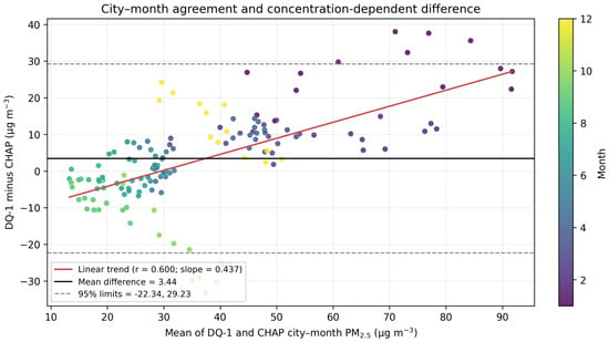
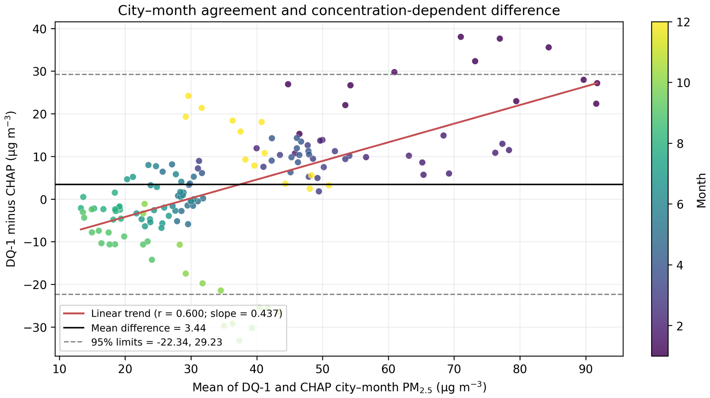
Figure 13. Bland–Altman agreement diagnostic for 143 city–month pairs. The solid black line is the mean DQ-1 minus CHAP difference; dashed lines are the mean difference ± 1.96 standard deviations. The fitted red line tests whether the difference varies with mean concentration, and color identifies month.

This distinction is deliberate. The full contextual model is used for descriptive interpolation at known 2024 grid cells and acquisition dates, whereas the strict model is used to estimate transfer when date and station identity are unavailable. The mapped products therefore answer where the contextual estimator places PM_2.5 within the sampled archive; they do not demonstrate that WSI radiometry alone transfers to a new year, region, or severe-pollution episode.

5.3. Methodological Contributions Relative to Previous Studies

First, the study provides a DQ-1-specific spectral-screening experiment rather than assuming a full-band input. All 15 channels and five spectral groups were compared using identical records, ancillary predictors, models, and pre-specified folds after H5-informed meteorological rematching and multispectral screening. Ten repeated balanced date-block allocations were then used to quantify ranking uncertainty. The results support a fold-sensitive operational choice of B3, not a statistically distinct or universal spectral optimum.

Second, the predictor design represents plausible RH growth, PBLH dilution, and wind ventilation through explicit feature engineering without labeling ExtraTrees as physically constrained. Under joint date–station blocking, adding B3 and its interactions to meteorology reduced ExtraTrees RMSE by 3.18%, whereas B3 alone had negative R². The contribution is therefore the quantified incremental value of WSI when conditioned on atmospheric state, not a claim that the spectral signal independently determines surface PM_2.5.

Third, the validation framework tests a more demanding transfer problem than randomly shuffled cross-validation. Dates and stations were independently partitioned, and each joint test cell was predicted from training data containing neither its date block nor its station block. ExtraTrees, XGBoost, and LightGBM were compared on the same 4210 BTH records and folds using WSI-only, meteorology-only, and combined inputs, with coordinates and calendar variables excluded. This design does not guarantee cross-year or cross-region performance, but it exposes record-wise optimism and provides a transparent simultaneous time–station transfer test.

Fourth, the mapped outputs are evaluated as coverage-dependent observations rather than gap-free monthly truth. The maps report contributing-scene counts across 11 available months, and CHAP consistency is examined at pixel–month and city–month scales, followed by two-way city–month decomposition and Bland–Altman analysis. This separates seasonal covariance, persistent city effects, and concentration-dependent discrepancies. Because CHAP shares monitoring and meteorological information and represents complete months, the comparison is explicitly product-to-product rather than independent validation.

5.4. Limitations and Future Work

Five limitations are central. First, the one-year BTH archive and modest blocked scores limit temporal and geographic generalization. Second, the full contextual mapping configuration includes coordinates and calendar encodings; its within-archive score is not transferable evidence, and the stricter coordinate- and calendar-free benchmark is substantially lower. Third, a baseline-to-full-model contrast combines band reduction, feature engineering, calendar terms, and a leaf-size change; staged ablation is required to separate these effects and shows that calendar terms account for most of the gain. Fourth, single-band rankings were unstable across repeated date partitions, and B3 should not be interpreted as a statistically superior wavelength. Fifth, only 1.61% of records exceeded 200 μg m⁻³ and severe episodes were strongly underestimated. No temporally matched 2024 MAIAC or official DQ-1 AOD was available for this run; future work should test independent years and regions, event-block validation, calibrated radiometry, official AOD, and uncertainty-aware models under identical blocked folds.

The supplied archive contains no November WSI scene, while October and December contain only four and three scene records. The products are therefore available-observation summaries. Future work should add independent years and regions, leave-one-pollution-event-out and year-block validation, uncertainty intervals from quantile forests or conformal prediction, geometry-normalized radiometry, validated cloud masks, official AOD, and monitoring sites excluded from all model development. These steps are required before the composites can support exposure or regulatory applications.

5.5. Interpretation of the CHAP Comparison

The CHAP comparison provides external product-level context, not independent validation. The pooled pixel–month correlation of 0.799 and city–month correlation of 0.830 indicate shared broad variability, but both systems use Chinese monitoring and meteorological information and differ in satellite input, modeling, spatial support, and temporal sampling. The 4.61 μg m⁻³ pooled and 3.44 μg m⁻³ city–month mean differences, together with nonzero RMSE, preclude treating the products as interchangeable.

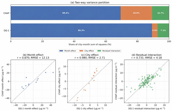
Two-way decomposition showed that month effects accounted for 89.3% of DQ-1 and 69.4% of CHAP city–month sums of squares, confirming that seasonal covariance dominates the raw correlation. Agreement was not purely seasonal: city effects had r = 0.980 and RMSE = 2.71 μg m⁻³, while residual city–month interactions retained r = 0.731 and RMSE = 4.18 μg m⁻³ after removing both month and city means. Month effects had r = 0.870 and RMSE = 12.13 μg m⁻³. Thus, residual correspondence remains, but the pooled correlation is materially inflated by the shared annual cycle (Figure 12).

Positive DQ-1 differences were largest in January and December, whereas October showed a substantial negative offset. Possible causes include incomplete within-month WSI sampling, 0.02° versus 1 km support, residual cloud and surface effects, lack of geometry normalization, distinct covariates, and CHAP smoothing. In particular, October averages only four WSI acquisition dates but a full CHAP calendar month; the −16.01 μg m⁻³ difference cannot be interpreted as calibration drift without daily CHAP fields matched to those dates.

The city–month Bland–Altman analysis gave a mean DQ-1 minus CHAP difference of 3.44 μg m⁻³ and empirical 95% limits from −22.34 to 29.23 μg m⁻³. Difference increased with pair mean (r = 0.600; slope = 0.437), demonstrating concentration-dependent disagreement and heteroscedasticity (Figure 13). The positive mean difference therefore does not summarize all seasons or concentration levels and does not establish interchangeability.

A stronger product comparison requires daily CHAP fields to construct composites on the exact DQ-1 acquisition dates, followed by area-weighted aggregation and evaluation against monitoring sites withheld from both modeling systems. Daily 2024 CHAP files were not present in the supplied archive, so an acquisition-matched October sampling-bias test could not be completed without introducing an unverified external dataset. The present monthly comparison is retained with this uncertainty stated explicitly; spatial-block bootstrap intervals should also be added when daily data become available.

6. Conclusions

The primary transfer assessment was the strict benchmark on 4210 BTH collocations, 65 stations, and 96 dates. ExtraTrees with WSI plus meteorology yielded R² = 0.1681 and RMSE = 34.84 μg m⁻³ under date grouping and R² = 0.1643 and RMSE = 34.92 μg m⁻³ under joint date–station blocking. Combined predictors outperformed meteorology only for all three algorithms, but B3 alone had non-positive skill. These coordinate- and calendar-free results support a conditional WSI increment within a meteorology-dominated estimator.

A separate full contextual configuration was used for within-2024 mapping and should not be compared directly with the strict transfer benchmark. It included B3, meteorology, physics-guided terms, grid coordinates, and calendar encodings and achieved date-grouped R² = 0.3919 and RMSE = 34.74 μg m⁻³. Controlled staging showed that the increase from R² = 0.1516 without coordinates/calendar to 0.3919 depended mainly on calendar information; neither band reduction nor physics-guided features independently explained the uncontrolled aggregate difference. Repeated date-block allocations also showed no stable single-band winner, so B3 is retained only as the pre-specified operational choice. Because B3 was retained only as the pre-specified split’s choice in the 2024 study archive, its suitability for a different year or region must be reassessed rather than assumed.

The contextual model generated estimates from 97 usable scenes and produced composites for January–October and December. Higher values occurred mainly over the southern and central plain, but uneven acquisition counts and screening mean that these are available-observation composites, not complete monthly or annual exposure fields. Date-blocked bias above 200 μg m⁻³ was −158.27 μg m⁻³, so the products are not suitable for severe-event exposure assessment. The principal methodological value lies in sensor-specific screening, verified meteorological timing, controlled attribution, joint date–station testing, and coverage-aware product evaluation, subject to the one-year domain and missing geometry-normalized reflectance and matched AOD.

Comparison with CHAP Version 4 monthly fields yielded pooled pixel–month r = 0.799 and RMSE = 13.68 μg m⁻³; the 143 city–month pairs yielded r = 0.830 and RMSE = 13.55 μg m⁻³. Two-way decomposition showed that seasonal covariance explained most DQ-1 city–month variance, although city effects and residual interactions remained correlated. Agreement was strong in several winter and spring months but weak in May and July, and October differed by −16.01 μg m⁻³. These findings provide product-level context while demonstrating substantial temporal-sampling and magnitude uncertainty.

References

- Pope, C.A.; Dockery, D.W. Health Effects of Fine Particulate Air Pollution: Lines That Connect. J. Air Waste Manag. Assoc. 2006, 56, 709–742. [Google Scholar] [CrossRef] [Scilit] [PubMed]
- Dominici, F.; Peng, R.D.; Bell, M.L.; Pham, L.; McDermott, A.; Zeger, S.L.; Samet, J.M. Fine Particulate Air Pollution and Hospital Admission for Cardiovascular and Respiratory Diseases. JAMA 2006, 295, 1127–1134. [Google Scholar] [CrossRef] [Scilit] [PubMed]
- Lelieveld, J.; Evans, J.S.; Fnais, M.; Giannadaki, D.; Pozzer, A. The Contribution of Outdoor Air Pollution Sources to Premature Mortality on a Global Scale. Nature 2015, 525, 367–371. [Google Scholar] [CrossRef] [Scilit] [PubMed]
- Ma, Z.; Hu, X.; Sayer, A.M.; Levy, R.; Zhang, Q.; Xue, Y.; Tong, S.; Bi, J.; Huang, L.; Liu, Y. Satellite-Based Spatiotemporal Trends in PM2.5 Concentrations: China, 2004–2013. Environ. Health Perspect. 2016, 124, 184–192. [Google Scholar] [CrossRef] [Scilit] [PubMed]
- van Donkelaar, A.; Martin, R.V.; Brauer, M.; Kahn, R.; Levy, R.; Verduzco, C.; Villeneuve, P.J. Global Estimates of Ambient Fine Particulate Matter Concentrations from Satellite-Based Aerosol Optical Depth: Development and Application. Environ. Health Perspect. 2010, 118, 847–855. [Google Scholar] [CrossRef] [Scilit] [PubMed]
- World Health Organization. WHO Global Air Quality Guidelines: Particulate Matter (PM2.5 and PM10), Ozone, Nitrogen Dioxide, Sulfur Dioxide and Carbon Monoxide; World Health Organization: Geneva, Switzerland, 2021. [Google Scholar]
- Burnett, R.; Chen, H.; Szyszkowicz, M.; Fann, N.; Hubbell, B.; Pope, C.A., 3rd; Apte, J.S.; Brauer, M.; Cohen, A.; Weichenthal, S.; et al. Global Estimates of Mortality Associated with Long-Term Exposure to Outdoor Fine Particulate Matter. Proc. Natl. Acad. Sci. USA 2018, 115, 9592–9597. [Google Scholar] [CrossRef] [Scilit] [PubMed]
- Brauer, M.; Amann, M.; Burnett, R.T.; Cohen, A.; Dentener, F.; Ezzati, M.; Henderson, S.B.; Krzyzanowski, M.; Martin, R.V.; Van Dingenen, R.; et al. Exposure Assessment for Estimation of the Global Burden of Disease Attributable to Outdoor Air Pollution. Environ. Sci. Technol. 2012, 46, 652–660. [Google Scholar] [CrossRef] [Scilit] [PubMed]
- Martin, R.V. Satellite Remote Sensing of Surface Air Quality. Atmos. Environ. 2008, 42, 7823–7843. [Google Scholar] [CrossRef] [Scilit]
- van Donkelaar, A.; Martin, R.V.; Brauer, M.; Boys, B.L. Use of Satellite Observations for Long-Term Exposure Assessment of Global Concentrations of Fine Particulate Matter. Environ. Health Perspect. 2015, 123, 135–143. [Google Scholar] [CrossRef] [Scilit] [PubMed]
- van Donkelaar, A.; Martin, R.V.; Brauer, M.; Hsu, N.C.; Kahn, R.A.; Levy, R.C.; Lyapustin, A.; Sayer, A.M.; Winker, D.M. Global Estimates of Fine Particulate Matter Using a Combined Geophysical-Statistical Method with Information from Satellites, Models, and Monitors. Environ. Sci. Technol. 2016, 50, 3762–3772. [Google Scholar] [CrossRef] [Scilit] [PubMed]
- Wei, J.; Huang, W.; Li, Z.; Xue, W.; Peng, Y.; Sun, L.; Cribb, M. Estimating 1-km-Resolution PM2.5 Concentrations across China Using the Space-Time Random Forest Approach. Remote Sens. Environ. 2019, 231, 111221. [Google Scholar] [CrossRef] [Scilit]
- Wei, J.; Li, Z.; Cribb, M.; Huang, W.; Xue, W.; Sun, L.; Guo, J.; Peng, Y.; Li, J.; Lyapustin, A.; et al. Improved 1 km Resolution PM2.5 Estimates across China Using Enhanced Space–Time Extremely Randomized Trees. Atmos. Chem. Phys. 2020, 20, 3273–3289. [Google Scholar] [CrossRef] [Scilit]
- Tian, Z.; Wei, J.; Li, Z. How Important Is Satellite-Retrieved Aerosol Optical Depth in Deriving Surface PM2.5 Using Machine Learning? Remote Sens. 2023, 15, 3780. [Google Scholar] [CrossRef] [Scilit]
- Wei, J.; Li, Z.; Lyapustin, A.; Sun, L.; Peng, Y.; Xue, W.; Su, T.; Cribb, M. Reconstructing 1-km-Resolution High-Quality PM2.5 Data Records from 2000 to 2018 in China: Spatiotemporal variations and policy implications. Remote Sens. Environ. 2021, 252, 112136. [Google Scholar] [CrossRef] [Scilit]
- Xue, W.; Wei, J.; Zhang, J.; Sun, L.; Che, Y.; Yuan, M.; Hu, X. Inferring Near-Surface PM2.5 Concentrations from the VIIRS Deep Blue Aerosol Product in China: A Spatiotemporally Weighted Random Forest Model. Remote Sens. 2021, 13, 505. [Google Scholar] [CrossRef] [Scilit]
- Kloog, I.; Koutrakis, P.; Coull, B.A.; Lee, H.J.; Schwartz, J. Assessing Temporally and Spatially Resolved PM2.5 Exposures for Epidemiological Studies Using Satellite Aerosol Optical Depth Measurements. Atmos. Environ. 2011, 45, 6267–6275. [Google Scholar] [CrossRef] [Scilit]
- Lee, H.J.; Liu, Y.; Coull, B.A.; Schwartz, J.; Koutrakis, P. A Novel Calibration Approach of MODIS AOD Data to Predict PM2.5 Concentrations. Atmos. Chem. Phys. 2011, 11, 7991–8002. [Google Scholar] [CrossRef] [Scilit]
- Chang, H.H.; Hu, X.; Liu, Y. Calibrating MODIS Aerosol Optical Depth for Predicting Daily PM2.5 Concentrations via Statistical Downscaling. J. Expo. Sci. Environ. Epidemiol. 2014, 24, 398–404. [Google Scholar] [CrossRef] [Scilit] [PubMed]
- Kloog, I.; Sorek-Hamer, M.; Lyapustin, A.; Coull, B.; Wang, Y.; Just, A.C.; Schwartz, J.; Broday, D.M. Estimating Daily PM2.5 and PM10 across the Complex Geo-Climate Region of Israel Using MAIAC Satellite-Based AOD Data. Atmos. Environ. 2015, 122, 409–416. [Google Scholar] [CrossRef] [Scilit] [PubMed]
- Ma, Z.; Hu, X.; Huang, L.; Bi, J.; Liu, Y. Estimating Ground-Level PM2.5 in China Using Satellite Remote Sensing. Environ. Sci. Technol. 2014, 48, 7436–7444. [Google Scholar] [CrossRef] [Scilit] [PubMed]
- Song, W.; Jia, H.; Huang, J.; Zhang, Y. A Satellite-Based Geographically Weighted Regression Model for Regional PM2.5 Estimation over the Pearl River Delta Region in China. Remote Sens. Environ. 2014, 154, 1–7. [Google Scholar] [CrossRef] [Scilit]
- Chen, G.; Li, S.; Knibbs, L.D.; Hamm, N.A.S.; Cao, W.; Li, T.; Guo, J.; Ren, H.; Abramson, M.J.; Guo, Y. A Machine Learning Method to Estimate PM2.5 Concentrations across China with Remote Sensing, Meteorological and Land Use Information. Sci. Total Environ. 2018, 636, 52–60. [Google Scholar] [CrossRef] [Scilit] [PubMed]
- Xue, T.; Zheng, Y.; Tong, D.; Zheng, B.; Li, X.; Zhu, T.; Zhang, Q. Spatiotemporal Continuous Estimates of PM2.5 Concentrations in China, 2000–2016: A Machine Learning Method with Inputs from Satellites, Chemical Transport Model, and Ground Observations. Environ. Int. 2019, 123, 345–357. [Google Scholar] [CrossRef] [Scilit] [PubMed]
- Di, Q.; Amini, H.; Shi, L.; Kloog, I.; Silvern, R.; Kelly, J.; Sabath, M.B.; Choirat, C.; Koutrakis, P.; Lyapustin, A.; et al. An Ensemble-Based Model of PM2.5 Concentration across the Contiguous United States with High Spatiotemporal Resolution. Environ. Int. 2019, 130, 104909. [Google Scholar] [CrossRef] [Scilit] [PubMed]
- Murray, N.L.; Holmes, H.A.; Liu, Y.; Chang, H.H. A Bayesian Ensemble Approach to Combine PM2.5 Estimates from Statistical Models Using Satellite Imagery and Numerical Model Simulation. Environ. Res. 2019, 178, 108601, Corrigendum in Environ. Res. 2020, 183, 108952. [Google Scholar] [CrossRef] [Scilit] [PubMed]
- Chen, J.; Yin, J.; Zang, L.; Zhang, T.; Zhao, M. Stacking Machine Learning Model for Estimating Hourly PM2.5 in China Based on Himawari-8 Aerosol Optical Depth Data. Sci. Total Environ. 2019, 697, 134021. [Google Scholar] [CrossRef] [Scilit] [PubMed]
- Xu, Q.; Chen, X.; Yang, S.; Tang, L.; Dong, J. Spatiotemporal Relationship between Himawari-8 Hourly Columnar Aerosol Optical Depth and Ground-Level PM2.5 Mass Concentration in Mainland China. Sci. Total Environ. 2021, 765, 144241. [Google Scholar] [CrossRef] [Scilit] [PubMed]
- Wei, J.; Li, Z.; Pinker, R.T.; Wang, J.; Sun, L.; Xue, W.; Li, R.; Cribb, M. Himawari-8-Derived Diurnal Variations in Ground-Level PM2.5 Pollution across China Using the Fast Space-Time Light Gradient Boosting Machine (LightGBM). Atmos. Chem. Phys. 2021, 21, 7863–7880. [Google Scholar] [CrossRef] [Scilit]
- Levy, R.C.; Mattoo, S.; Munchak, L.A.; Remer, L.A.; Sayer, A.M.; Patadia, F.; Hsu, N.C. The Collection 6 MODIS Aerosol Products over Land and Ocean. Atmos. Meas. Tech. 2013, 6, 2989–3034. [Google Scholar] [CrossRef] [Scilit]
- Li, Z.; Zhao, X.; Kahn, R.; Mishchenko, M.; Remer, L.; Lee, K.-H.; Wang, M.; Laszlo, I.; Nakajima, T.; Maring, H. Uncertainties in Satellite Remote Sensing of Aerosols and Impact on Monitoring Its Long-Term Trend: A review and perspective. Ann. Geophys. 2009, 27, 2755–2770. [Google Scholar] [CrossRef] [Scilit]
- Lyapustin, A.; Martonchik, J.; Wang, Y.; Laszlo, I.; Korkin, S. Multiangle Implementation of Atmospheric Correction (MAIAC): 1. Radiative Transfer Basis and Look-Up Tables. J. Geophys. Res. Atmos. 2011, 116, D03210. [Google Scholar] [CrossRef] [Scilit]
- Lyapustin, A.; Wang, Y.; Laszlo, I.; Kahn, R.; Korkin, S.; Remer, L.; Levy, R.; Reid, J.S. Multiangle Implementation of Atmospheric Correction (MAIAC): 2. Aerosol Algorithm. J. Geophys. Res. Atmos. 2011, 116, D03211. [Google Scholar] [CrossRef] [Scilit]
- Lyapustin, A.I.; Wang, Y.; Laszlo, I.; Hilker, T.; Hall, F.G.; Sellers, P.J.; Tucker, C.J.; Korkin, S.V. Multi-Angle Implementation of Atmospheric Correction for MODIS (MAIAC): 3. Atmospheric Correction. Remote Sens. Environ. 2012, 127, 385–393. [Google Scholar] [CrossRef] [Scilit]
- Lyapustin, A.; Wang, Y.; Korkin, S.; Huang, D. MODIS Collection 6 MAIAC Algorithm. Atmos. Meas. Tech. 2018, 11, 5741–5765. [Google Scholar] [CrossRef] [Scilit]
- Lyapustin, A.; Wang, Y.; Frey, R. An Automatic Cloud Mask Algorithm Based on Time Series of MODIS Measurements. J. Geophys. Res. Atmos. 2008, 113, D16207. [Google Scholar] [CrossRef] [Scilit]
- Lyapustin, A.; Wang, Y.; Laszlo, I.; Korkin, S. Improved Cloud and Snow Screening in MAIAC Aerosol Retrievals Using Spectral and Spatial Analysis. Atmos. Meas. Tech. 2012, 5, 843–850. [Google Scholar] [CrossRef] [Scilit]
- Chudnovsky, A.; Tang, C.; Lyapustin, A.; Wang, Y.; Schwartz, J.; Koutrakis, P. A Critical Assessment of High-Resolution Aerosol Optical Depth Retrievals for Fine Particulate Matter Predictions. Atmos. Chem. Phys. 2013, 13, 10907–10917. [Google Scholar] [CrossRef] [Scilit]
- Shen, H.; Li, T.; Yuan, Q.; Zhang, L. Estimating Regional Ground-Level PM2.5 Directly from Satellite Top-of-Atmosphere Reflectance Using Deep Belief Networks. J. Geophys. Res. Atmos. 2018, 123, 13875–13886. [Google Scholar] [CrossRef] [Scilit]
- Liu, J.; Weng, F.; Li, Z. Satellite-Based PM2.5 Estimation Directly from Reflectance at the Top of the Atmosphere Using a Machine Learning Algorithm. Atmos. Environ. 2019, 208, 113–122. [Google Scholar] [CrossRef] [Scilit]
- Yang, L.; Xu, H.; Yu, S. Estimating PM2.5 Concentrations in the Yangtze River Delta Region of China Using Random Forest and Top-of-Atmosphere Reflectance. J. Environ. Manag. 2020, 272, 111061. [Google Scholar] [CrossRef] [Scilit] [PubMed]
- Bai, H.; Zheng, Z.; Zhang, Y.; Huang, H.; Wang, L. Comparison of Satellite-Based PM2.5 Estimation from Aerosol Optical Depth and Top-of-Atmosphere Reflectance. Aerosol Air Qual. Res. 2021, 21, 200257. [Google Scholar] [CrossRef] [Scilit]
- Mao, F.; Hong, J.; Min, Q.; Gong, W.; Zang, L.; Yin, J. Estimating Hourly Full-Coverage PM2.5 over China Based on TOA Reflectance Data from the Fengyun-4A Satellite. Environ. Pollut. 2021, 270, 116119. [Google Scholar] [CrossRef] [Scilit] [PubMed]
- Choi, H.; Park, S.; Kang, Y.; Im, J.; Song, S. Retrieval of Hourly PM2.5 Using Top-of-Atmosphere Reflectance from Geostationary Ocean Color Imagers I and II. Environ. Pollut. 2023, 323, 121169. [Google Scholar] [CrossRef] [Scilit] [PubMed]
- Wang, Z.; Zhang, R.; Chen, R.; Chen, H. The Aerosol Optical Depth Retrieval from Wide-Swath Imaging of DaQi-1 over Beijing. Atmosphere 2024, 15, 1476. [Google Scholar] [CrossRef] [Scilit]
- Dai, G.; Wu, S.; Long, W.; Liu, J.; Xie, Y.; Sun, K.; Meng, F.; Song, X.; Huang, Z.; Chen, W. Aerosol and Cloud Data Processing and Optical Property Retrieval Algorithms for the Spaceborne ACDL/DQ-1. Atmos. Meas. Tech. 2024, 17, 1879–1890. [Google Scholar] [CrossRef] [Scilit]
- Hersbach, H.; Bell, B.; Berrisford, P.; Hirahara, S.; Horányi, A.; Muñoz-Sabater, J.; Nicolas, J.; Peubey, C.; Radu, R.; Schepers, D.; et al. The ERA5 Global Reanalysis. Q. J. R. Meteorol. Soc. 2020, 146, 1999–2049. [Google Scholar] [CrossRef] [Scilit]
- Geurts, P.; Ernst, D.; Wehenkel, L. Extremely Randomized Trees. Mach. Learn. 2006, 63, 3–42. [Google Scholar] [CrossRef] [Scilit]
- He, Q.; Wang, M.; Yim, S.H.L. The Spatiotemporal Relationship between PM2.5 and Aerosol Optical Depth in China: Influencing Factors and Implications for Satellite PM2.5 Estimations Using MAIAC Aerosol Optical Depth. Atmos. Chem. Phys. 2021, 21, 18375–18391. [Google Scholar] [CrossRef] [Scilit]
- Rodriguez, J.D.; Perez, A.; Lozano, J.A. Sensitivity Analysis of k-Fold Cross Validation in Prediction Error Estimation. IEEE Trans. Pattern Anal. Mach. Intell. 2010, 32, 569–575. [Google Scholar] [CrossRef] [Scilit] [PubMed]
- Roberts, D.R.; Bahn, V.; Ciuti, S.; Boyce, M.S.; Elith, J.; Guillera-Arroita, G.; Hauenstein, S.; Lahoz-Monfort, J.J.; Schröder, B.; Thuiller, W.; et al. Cross-Validation Strategies for Data with Temporal, Spatial, Hierarchical, or Phylogenetic Structure. Ecography 2017, 40, 913–929. [Google Scholar] [CrossRef] [Scilit]
- Ploton, P.; Mortier, F.; Rejou-Mechain, M.; Barbier, N.; Picard, N.; Rossi, V.; Dormann, C.; Cornu, G.; Viennois, G.; Bayol, N.; et al. Spatial Validation Reveals Poor Predictive Performance of Large-Scale Ecological Mapping Models. Nat. Commun. 2020, 11, 4540. [Google Scholar] [CrossRef] [Scilit] [PubMed]
- HJ 618-2011; Determination of Atmospheric Particles PM10 and PM2.5 in Ambient Air by Gravimetric Method. Ministry of Environmental Protection: Beijing, China, 2011.
- Wei, J.; Li, Z.; Zhu, T. ChinaHighPM2.5 (2022–Present), Version 4; Zenodo: Geneve, Switzerland, 2026. [Google Scholar] [CrossRef]
- Bland, J.M.; Altman, D.G. Statistical Methods for Assessing Agreement between Two Methods of Clinical Measurement. Lancet 1986, 1, 307–310. [Google Scholar] [CrossRef] [Scilit]
- Ma, Z.; Liu, R.; Liu, Y.; Bi, J. Effects of Air Pollution Control Policies on PM2.5 Pollution Improvement in China from 2005 to 2017: A Satellite-Based Perspective. Atmos. Chem. Phys. 2019, 19, 6861–6877. [Google Scholar] [CrossRef] [Scilit]
- Chen, T.; Guestrin, C. XGBoost: A Scalable Tree Boosting System. In Proceedings of the 22nd ACM SIGKDD International Conference on Knowledge Discovery and Data Mining, San Francisco, CA, USA, 13–17 August 2016; pp. 785–794. [Google Scholar] [CrossRef] [Scilit]
- Ke, G.; Meng, Q.; Finley, T.; Wang, T.; Chen, W.; Ma, W.; Ye, Q.; Liu, T.-Y. LightGBM: A Highly Efficient Gradient Boosting Decision Tree. In Proceedings of the Advances in Neural Information Processing Systems 30, Long Beach, CA, USA, 4–9 December 2017; pp. 3146–3154. [Google Scholar]
Disclaimer/Publisher’s Note: The statements, opinions and data contained in all publications are solely those of the individual author(s) and contributor(s) and not of MDPI and/or the editor(s). MDPI and/or the editor(s) disclaim responsibility for any injury to people or property resulting from any ideas, methods, instructions or products referred to in the content. |
© 2026 by the authors. Licensee MDPI, Basel, Switzerland. This article is an open access article distributed under the terms and conditions of the Creative Commons Attribution (CC BY) license.