Daily Lake-Surface NDVI Reconstruction Using Multi-Source Machine Learning Under Incomplete Optical Observations

Highlights

What are the main findings?

• A dual-situation CatBoost framework generated spatially continuous daily lake-surface NDVI fields across regions with and without coincident GNSS-R observations.
• GNSS-R observables provided complementary information beyond meteorological and geographic predictors on the same matched sample domain.

What are the implications of the main findings?

• The reconstructed NDVI record revealed frequent positive-NDVI surface signals during 2018–2021 and generally weaker signals after 2022.
• The framework supports long-term analysis of lake-surface NDVI dynamics under incomplete optical observation conditions.

Abstract

Accurate and continuous monitoring of cyanobacterial blooms is essential for lake ecosystem management, but optical remote-sensing observations are frequently limited by cloud contamination and illumination conditions. To address this limitation, this study proposes a multi-source machine learning framework for daily lake-surface normalized difference vegetation index (NDVI) reconstruction under missing optical observations by integrating Cyclone Global Navigation Satellite System (CYGNSS) observations, ERA5-Land meteorological variables, geographic coordinates, and the CatBoost (version 1.2.10) regression algorithm. Lake Taihu and Lake Chaohu, two representative eutrophic lakes in eastern China, were selected as study areas. An ablation analysis was conducted to evaluate the contributions of different predictor groups. Under the random within-domain evaluation, the full-feature model combining GNSS-R observables, meteorological variables, and geographic coordinates achieved an average test $R^2$ of 0.63 and a root mean square error (RMSE) of 0.15 in GNSS-R-covered regions. Compared with the model using meteorological variables and geographic coordinates alone, the inclusion of GNSS-R observables provided additional predictive information, indicating that GNSS-R served as a supplementary rather than dominant information source. In regions without GNSS-R coverage, meteorological variables and geographic coordinates were used to maintain spatially continuous NDVI reconstruction over the lake surface. The annual results show that the framework can generate daily reconstructed NDVI estimates for both lakes within the study domain. Cross-product comparison with Fengyun-3F (FY-3F) NDVI indicated broad consistency in the major spatial patterns of lake-surface high-NDVI signals, particularly in open-water areas. However, differences in spatial resolution and temporal compositing limit direct pixel-level assessment. Interannual analysis suggested that the frequency and magnitude of positive-NDVI surface signals generally decreased after 2022; however, these signals should be interpreted as integrated lake-surface ecological responses rather than direct quantitative indicators of cyanobacterial bloom intensity. A Shapley Additive Explanations (SHAP) analysis showed that geographic coordinates, GNSS-R surface reflectivity, temperature, and wind speed contributed to the model predictions. Overall, the proposed framework provides a lake-specific empirical approach for maintaining spatially continuous daily NDVI information when optical observations are incomplete.

1. Introduction

Lakes play a vital role in maintaining ecosystem stability, regulating greenhouse gas fluxes, sustaining biodiversity, and providing essential freshwater resources [1,2,3]. However, rapid industrialization, urban expansion, and intensive agriculture have accelerated nutrient loading and eutrophication, increasing the occurrence of harmful algal blooms (HABs) worldwide [4]. Although phytoplankton are fundamental to aquatic primary production, carbon cycling, and food-web functioning, bloom-forming taxa such as cyanobacteria can produce toxins that accumulate through the food chain, threatening aquatic organisms, ecosystem health, and human well-being [5,6,7]. Dense HABs can also reduce light penetration, suppress underwater photosynthesis, and intensify oxygen depletion, thereby destabilizing aquatic ecosystems [8]. Therefore, effective monitoring of cyanobacterial blooms is essential for ecological risk assessment, water quality protection, and sustainable lake management.

Optical remote sensing has become one of the most widely used approaches for cyanobacterial bloom monitoring, and indices such as the Normalized Difference Vegetation Index (NDVI) are effective for characterizing bloom extent, intensity, and spatiotemporal dynamics [9,10]. However, the utility of optical observations is fundamentally constrained by cloud cover and illumination conditions. Under cloudy weather or at night, optical sensors cannot provide reliable observations, which severely limits their ability to capture rapidly changing bloom events. For example, a severe cyanobacterial bloom in Lake Taihu in May 2007 was not adequately observed by optical satellites because of adverse weather conditions, thereby hampering timely disaster response [11]. Similarly, although [12] revealed the widespread occurrence and long-term increase in algal blooms in global freshwater lakes using Landsat imagery, their analysis still reflected the inherent limitations of optical remote sensing for high-frequency and short-term monitoring. Because cyanobacterial blooms can change rapidly over short timescales, these data gaps are not merely a technical inconvenience but a major obstacle to understanding bloom dynamics. Therefore, the key need is to reconstruct temporally continuous and spatially reliable NDVI observations when optical data are missing.

A variety of methods have been developed to reconstruct missing optical remote-sensing observations, including approaches based on spatial, spectral, and temporal information [13,14]. However, spatial- and spectral-based methods often struggle in large areas covered by thick clouds [15], while temporal reconstruction methods generally rely on the assumption that surface conditions vary only slightly within a limited time window [16,17,18]. This assumption is often unsuitable for cyanobacterial blooms, whose distribution and intensity can change rapidly in response to meteorological forcing and lake-surface processes. As noted by [19], temporal reconstruction methods remain inadequate for applications requiring high timeliness and observation frequency. Consequently, optical remote sensing alone cannot fully satisfy the need for continuous bloom monitoring, and a complementary observation source is required.

Microwave remote sensing, with its all-weather and all-day observational capability, provides an important complement to optical remote sensing [20,21]. Among microwave techniques, Global Navigation Satellite System-Reflectometry (GNSS-R) has shown potential for characterizing inland-water surface conditions and for supporting empirical analyses of water-quality and bloom-related phenomena [22,23,24,25,26]. In particular, the Cyclone Global Navigation Satellite System (CYGNSS) provides passive observations with relatively frequent but irregular sampling, making it a potentially useful auxiliary data source for aquatic monitoring [27]. Previous studies have explored the use of CYGNSS for cyanobacterial bloom detection in Lake Taihu [25], for improving bloom-related classification by incorporating meteorological variables and machine learning methods [24], and for empirically reconstructing missing lake-surface NDVI using CYGNSS observations and meteorological predictors [26]. It is important, however, to distinguish between direct optical NDVI retrieval and GNSS-R-assisted statistical reconstruction. NDVI is derived from red and near-infrared reflectance, whereas GNSS-R observables are primarily affected by lake-surface roughness, observation geometry, signal coherence, and dielectric properties. Therefore, GNSS-R does not directly measure optical NDVI, and any association between GNSS-R observables and NDVI should be interpreted as indirect and condition-dependent. In bloom-prone shallow lakes, meteorological and hydrodynamic conditions may simultaneously influence cyanobacterial surface accumulation, optical NDVI, and microwave surface scattering, thereby producing statistical covariance among these variables. In addition, existing GNSS-R-assisted approaches remain constrained by the sparse and irregular distribution of specular reflection points over lake surfaces, which limits their ability to independently produce spatially continuous NDVI fields across an entire lake. Thus, in the present study, GNSS-R is treated as a supplementary predictor rather than a dominant or direct source of NDVI information.

These complementary strengths and weaknesses indicate that neither optical remote sensing nor GNSS-R, when used in isolation, is sufficient for spatially continuous and temporally frequent lake-surface NDVI monitoring. Optical data provide direct spectral support for NDVI estimation but are often affected by cloud-contaminated gaps, whereas GNSS-R enables observations under unfavorable weather and illumination conditions but remains spatially sparse over lake surfaces. Therefore, the central challenge is to integrate multiple observation sources in a way that balances temporal continuity, spatial completeness, and environmental interpretability [28].

Zhen and Yan [26] showed that missing lake-surface NDVI under cloudy conditions could be recovered using CYGNSS observations, meteorological data, and a Bagging Tree model. That study mainly examined the feasibility and accuracy of GNSS-R-assisted NDVI recovery, as well as the effective range of GNSS-R observations. In the present study, the reconstruction is extended to the entire lake surface using a dual-situation modeling strategy. GNSS-R variables, meteorological variables, and geographic coordinates were used in areas with GNSS-R observations, while meteorological variables and geographic coordinates were used elsewhere. The framework was further applied to both Lake Taihu and Lake Chaohu.

The main contributions of this study are threefold. First, a dual-situation NDVI reconstruction framework was developed to integrate sparse GNSS-R observations where available while maintaining spatial continuity across the lake surface. Second, model-derived uncertainty information was incorporated into the reconstructed NDVI products to indicate their relative spatial and temporal reliability, rather than providing deterministic estimates alone. Third, the reconstructed NDVI fields were examined through a cross-product spatial consistency comparison with FY-3F NDVI products and an ecological consistency check using in situ water-quality observations.

2. Materials and Methods

2.1. Research Area

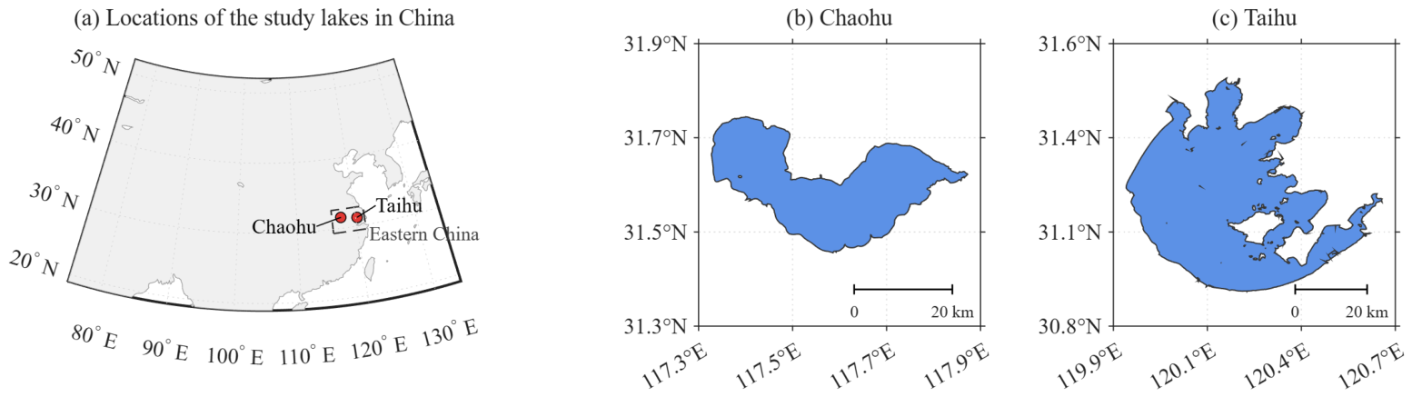
Lake Taihu and Lake Chaohu, two representative shallow eutrophic lakes in eastern China with recurrent cyanobacterial blooms, were selected as the study areas. The two lakes share similar bloom-prone characteristics, including high nutrient loading, shallow water depth, and strong anthropogenic influences, while differing in lake size, morphology, hydrodynamic conditions, and bloom patterns. These similarities and differences provide a basis for examining the within-lake performance of the framework under two different lake settings. Key characteristics of the study lakes are summarized in

Table 1. Summary of the study lakes.

Lake	Coordinates	Climate	Type	Main Bloom Conditions
Taihu	30°55′–31°33′ N; 119°52′–120°36′ E	Subtropical monsoon	Large shallow freshwater lake	Eutrophication; calm water; wind accumulation
Chaohu	31°25′–31°43′ N; 117°16′–117°51′ E	Subtropical monsoon	Shallow eutrophic freshwater lake	High nutrient loading; warm conditions; low wind

and Figure 1.

2.2. Datasets

This study integrates satellite, meteorological, and in situ datasets to support NDVI reconstruction under missing optical observations, model interpretation, and consistency assessment. CYGNSS GNSS-R observations were used to characterize lake-surface scattering conditions, Moderate Resolution Imaging Spectroradiometer (MODIS) Terra/Aqua surface reflectance data were used to derive reference NDVI, and ERA5-Land data provided meteorological forcing variables related to bloom development. In addition, FY-3F NDVI products were used for external spatial comparison, while water-quality observations from 14 monitoring stations in Lake Taihu were used to examine ecological consistency between the final reconstructed NDVI series and measured nutrient and chlorophyll conditions. A summary of all datasets is provided in

Table 2. Summary of the datasets used in this study.

Data Type	Product, Variables, and Role
GNSS-R	CYGNSS L1 v3.2; surface reflectivity (SR), incidence angle, signal-to-noise ratio (SNR), and acquisition time; auxiliary predictors representing lake-surface scattering and observation conditions.
Optical remote sensing	MOD09GA/MYD09GA; 500 m daily red and near-infrared bands; reference NDVI calculation.
Meteorology	ERA5-Land; 0.1° hourly temperature, pressure, wind, precipitation, and radiation; environmental predictors.
Cross-product comparison	FY-3F NDVI; 1000 m 10-day NDVI product; cross-product spatial consistency comparison.
In situ	Taihu monitoring stations; quarterly nitrogen, phosphorus, and chlorophyll-a; ecological consistency check.

.

2.3. Data Processing

In the data preprocessing phase, quality control was initially applied to the CYGNSS data by removing observations with an incidence angle ≥ 65°, antenna gain ≤ 0, and SNR ≤ 1 to ensure the reliability of the dataset. Subsequently, using the band information from the MOD09GA and MYD09GA products, which indicate pixel quality, we excluded pixels affected by cloud cover and cloud shadows, retaining only high-quality pixels. Given the rapid fluctuations in cyanobacteria dynamics and the advantage of obtaining two MODIS images per day, we computed the average of the two daily images as the reference NDVI value.

Considering the need to integrate heterogeneous multi-source datasets, careful spatiotemporal matching is required. CYGNSS observations are acquired at discrete specular points along satellite tracks, and each observation represents an integrated surface-reflection response over a geometry- and coherence-dependent footprint rather than an infinitesimal point. In contrast, ERA5-Land and MODIS NDVI are provided as gridded raster datasets. In terms of temporal sampling, CYGNSS observations over an individual lake are irregular and do not have a fixed revisit interval, ERA5-Land provides hourly data, MODIS provides two nominal daytime observations per day, typically around 10:30 AM and 1:30 PM local time, and the Medium Resolution Spectral Imager (MERSI) NDVI has a ten-day temporal resolution. In terms of spatial sampling, under nominal coherent-reflection conditions, a CYGNSS observation after July 2019 has been reported to correspond to an approximate footprint of 0.5 km × 3.5 km. However, the actual footprint may vary with observation geometry, surface roughness, and signal coherence and should not be interpreted as a fixed spatial resolution. ERA5-Land, MODIS NDVI, and MERSI NDVI have nominal spatial resolutions of $0.1°\times 0.1°$, 500 m × 500 m, and 1000 m × 1000 m, respectively. ERA5-Land and MODIS are provided on regular geographic grids, whereas the MERSI product uses the Hammer projection and was therefore transformed to a common geographic coordinate system before matching.

For spatiotemporal alignment, latitude and longitude were used as the common geographic reference. To link the discrete CYGNSS observations with the MODIS grid, a local matching window of $0.01°$ in both latitude and longitude was defined around each specular point. The window size was determined empirically through a preliminary sensitivity analysis using the 2019 Lake Chaohu dataset. Among the tested window sizes, $0.01°$ provided the best overall model performance, with relatively high $R^2$ and low RMSE, mean squared error, and mean absolute error, and was therefore adopted consistently for both Lake Chaohu and Lake Taihu. This value serves only as a spatial matching criterion and does not represent the physical footprint or spatial resolution of CYGNSS observations. The actual CYGNSS scattering footprint is typically elongated and direction-dependent because of the delay–Doppler geometry. Therefore, the square geographic matching window may not fully represent the true footprint geometry and may introduce spatial mismatch for some observations.

All valid MODIS NDVI pixels within this window were assigned the corresponding CYGNSS observables, including surface reflectivity (SR), signal-to-noise ratio (SNR), incidence angle, and acquisition time, and were used to construct the matched GNSS-R–NDVI samples. This fixed-window strategy provides a consistent empirical approach for associating CYGNSS observations with MODIS pixels. In the matched dataset used in this study, adjacent CYGNSS specular points were separated sufficiently to avoid assigning more than one GNSS-R observation to the same MODIS pixel, thereby maintaining unique sample pairing.

For temporal matching, all acquisition times were expressed in Coordinated Universal Time (UTC). CYGNSS observations collected between 00:00 and 08:00 UTC each day were selected, corresponding to 08:00–16:00 China Standard Time (UTC+8) over Lake Taihu and Lake Chaohu. This interval encompasses the nominal daytime overpass periods of MODIS Terra and Aqua while retaining a sufficient number of CYGNSS specular-point observations for model training and NDVI reconstruction under missing optical observations. The CYGNSS and MODIS observations were matched at the daily scale rather than through exact simultaneous acquisition; therefore, residual within-day temporal differences between the two datasets may introduce additional uncertainty. The daily reference NDVI was calculated by averaging the valid Terra and Aqua NDVI observations after removing pixels affected by clouds and cloud shadows.

To achieve spatial consistency among the multi-source datasets, ERA5-Land and FY-3F/MERSI NDVI data were resampled to match the spatial resolution of the MODIS NDVI grid using bilinear interpolation. This interpolation was used only for spatial resampling and grid alignment. It did not introduce additional fine-scale physical or statistical information and therefore served only as a preprocessing step. After these procedures, the CYGNSS, MODIS, ERA5-Land, and FY-3F/MERSI datasets were aligned in space and time for subsequent modeling and consistency assessment.

This potential spatial mismatch, particularly near shorelines or complex water–land boundaries, represents an additional source of uncertainty in the overall reconstruction process and was considered qualitatively when interpreting the model-derived uncertainty maps and consistency comparisons.

Given the limited spatial coverage of CYGNSS specular points over lake surfaces, a dual-situation modeling strategy was adopted. In GNSS-R-covered regions, GNSS-R observables, ERA5-Land meteorological variables, and geographic coordinates were used as input features to predict missing NDVI values. In regions without GNSS-R observations, meteorological variables and geographic coordinates were used as input features to maintain spatially continuous NDVI reconstruction. This design allows the framework to use GNSS-R surface-reflection information where available, while preserving lake-wide spatial continuity in non-covered regions.

2.4. Categorical Boosting Regression Algorithm

Daily lake-surface NDVI reconstruction under missing optical observations was formulated as a supervised pixel-level regression problem, in which multi-source predictors were used to estimate missing NDVI values over the lake surface. CatBoost was selected as the regression algorithm because it is well suited to modeling nonlinear relationships among heterogeneous predictors. CatBoost is a gradient-boosting decision-tree algorithm that incorporates mechanisms such as ordered boosting to reduce prediction shift and improve robustness under complex nonlinear feature interactions [29,30].

For each sample i, let ${\mathbf{x}}_i$ denote the input feature vector and let $y_i$ denote the corresponding reference NDVI derived from MODIS. In this study, ${\mathbf{x}}_i$ contains GNSS-R observables, meteorological variables, and geographic information, while $y_i$ represents the target NDVI value to be predicted. Each sample corresponds to one target pixel, and neighboring NDVI values were not directly included as model inputs, although latitude and longitude provided implicit spatial-location information. Given a training dataset

$$D={\left\{({\mathbf{x}}_i,y_i)\right\}}_{i=1}^n,$$

(1)

where n is the number of training samples, the CatBoost regression model can be expressed as

$${\widehat{y}}_i=f\left({\mathbf{x}}_i\right)={\displaystyle \sum _{m=1}^M}{f}_m\left({\mathbf{x}}_i\right),$$

(2)

where ${\widehat{y}}_i$ is the predicted NDVI for sample i, M is the total number of boosting iterations (i.e., the number of decision trees), and $f_m\left({\mathbf{x}}_i\right)$ is the output of the m-th tree for the input feature vector ${\mathbf{x}}_i$.

In a conventional CatBoost regression setting, the prediction error can be measured using the root mean square error (RMSE),

$$L_{\mathrm{RMSE}}={\left[{\displaystyle \frac{1}{n}}{\displaystyle \sum _{i=1}^n}{\left(y_i-{\widehat{y}}_i\right)}^2\right]}^{1/2}.$$

(3)

For the standard boosting process, at iteration t, a new decision tree is fitted to the current residuals,

$$r_i^{\left(t\right)}=-{\displaystyle \frac{\partial L_{\mathrm{RMSE}}\left(y_i,{\widehat{y}}_i^{(t-1)}\right)}{\partial {\widehat{y}}_i^{(t-1)}}}\propto y_i-{\widehat{y}}_i^{(t-1)},$$

(4)

and the prediction is updated as

$${\widehat{y}}_i^{\left(t\right)}={\widehat{y}}_i^{(t-1)}+\eta f_t\left({\mathbf{x}}_i\right),$$

(5)

where $\eta$ is the learning rate and $t=1,2,\dots ,M$ denotes the iteration index.

For each lake and each year, the matched samples were randomly divided into training, validation, and test sets at a ratio of 6:2:2. The training set was used to fit the CatBoost regression model, the validation set was used for model selection and early stopping, and the test set was used to evaluate model performance within the corresponding lake-year sample domain. The same splitting strategy was applied independently to the GNSS-R-covered and non-GNSS-R-covered situations.

The numbers of samples available for each lake-year and modeling situation are summarized in

Table 3. Number of samples used for the GNSS-R-covered and non-GNSS-R-covered modeling situations for Lake Taihu and Lake Chaohu from 2018 to 2024.

Lake	Year	GNSS-R-Covered Samples	Non-GNSS-R-Covered Samples
Taihu	2018	5185	631,788
	2019	17,165	1,206,335
	2020	20,748	1,026,089
	2021	19,292	1,085,834
	2022	13,565	1,111,146
	2023	18,332	1,021,934
	2024	10,207	993,184
Chaohu	2018	1514	225,916
	2019	5554	412,501
	2020	4466	345,872
	2021	9074	379,252
	2022	6111	405,353
	2023	6554	362,967
	2024	4575	349,208

. The GNSS-R-covered sample sets were substantially smaller than the non-GNSS-R-covered sample sets because the former were restricted to MODIS pixels that could be matched with valid CYGNSS observations, whereas the latter included valid pixels without coincident GNSS-R observations.

Because the objective of this study was to reconstruct daily lake-surface NDVI within the observed lake domains, the reported accuracy primarily reflects within-domain interpolation capability rather than independent spatial or temporal extrapolation or transferability across different lakes.

To further assess the potential influence of temporal dependence introduced by random sample splitting, an additional week-based sensitivity analysis was conducted using the 2018–2024 datasets for both lakes and both reconstruction situations. Daily observations were grouped by calendar week, and all samples within the same week were assigned entirely to the training, validation, or test subset while maintaining an approximately 6:2:2 sample ratio. This design reduces the likelihood that observations from the same short-term temporal window are distributed across different subsets. Because adjacent weeks may still be assigned to different subsets, this analysis was used to test the sensitivity of model performance to temporal grouping.

The CatBoost regression model was configured with a maximum of 2000 boosting iterations, a learning rate of 0.03, and a tree depth of 14. Early stopping was enabled based on the validation set with a patience of 100 iterations. The RMSEWithUncertainty objective was adopted with posterior sampling enabled. RMSE was used to evaluate prediction accuracy, while the final reconstruction models were trained using the RMSEWithUncertainty objective to obtain both NDVI estimates and model-derived uncertainty, as described in Section 2.5.

Compared with conventional boosting methods, CatBoost introduces ordered boosting to reduce prediction shift during training and improve robustness under complex feature interactions [30]. This property is useful for the present NDVI reconstruction problem because the statistical relationships between the multi-source predictors and MODIS NDVI are nonlinear. In this study, CatBoost was used to model these empirical relationships within each lake-year sample domain.

Furthermore, the trained CatBoost model was interpreted using SHAP, which quantifies the contribution of each predictor to the fitted model output based on cooperative game theory. In this study, SHAP was used to examine how strongly the model relied on different predictors and how predictor values were statistically associated with the predicted NDVI. SHAP values were not interpreted as evidence of causal or direct physical effects on NDVI.

2.5. Uncertainty Quantification

In addition to NDVI prediction, the final CatBoost models were trained using the RMSEWithUncertainty objective with posterior sampling enabled. Prediction uncertainty was obtained using the CatBoost virtual-ensemble method with 20 virtual ensembles. For each input sample, the method returned a mean NDVI prediction, a knowledge-uncertainty component, and a data-uncertainty component.

The total predictive variance was calculated as

$$u_{i,\mathrm{total}}=u_{i,\mathrm{k}}+u_{i,\mathrm{d}},$$

(6)

where $u_{i,\mathrm{k}}$ and $u_{i,\mathrm{d}}$ denote the knowledge- and data-uncertainty components, respectively. The corresponding total predictive standard deviation was calculated as

$${\sigma }_{i,\mathrm{total}}=\sqrt{max\left(u_{i,\mathrm{total}},0\right)},$$

(7)

where the maximum operation was used to avoid taking the square root of small negative values caused by numerical errors.

For visualization, relative uncertainty was calculated as

$$U_{i,\mathrm{relative}}={\displaystyle \frac{{\sigma }_{i,\mathrm{total}}}{y_{max}-y_{min}}},$$

(8)

where $y_{max}-y_{min}$ is the NDVI range calculated from all samples in the corresponding lake-year modeling dataset. Relative uncertainty represents the total predictive standard deviation normalized by the observed NDVI range and is therefore a dimensionless quantity. It does not represent an absolute error probability.

3. Results

3.1. Ablation Analysis and Dual-Situation Modeling Basis

Three categories of predictors were employed as model inputs. The first category consisted of GNSS-R observables, including SNR, SR, incidence angle, and acquisition time, while the second category included ERA5-Land meteorological variables, such as temperature, surface pressure, wind speed, wind direction, downward solar radiation, and precipitation. In addition, latitude and longitude were included as geographic location encodings to represent persistent within-lake spatial patterns.

To evaluate the statistical contribution of different predictor groups, an ablation experiment was conducted using samples for which GNSS-R observations were available. Five feature combinations were examined: G+M+C, G+M, M only, M+C, and G only, where G, M, and C denote GNSS-R observables, meteorological variables, and geographic coordinates, respectively. All feature combinations were evaluated on the same GNSS-R-matched sample domain using the same training, validation, and test splitting strategy. As shown in

Table 4. Overall average ablation results evaluated on GNSS-R-matched samples across Lake Taihu and Lake Chaohu from 2018 to 2024.

Features	Train		Validation		Test
	${\mathit{R}}^{\mathbf{2}}$	RMSE	${\mathit{R}}^{\mathbf{2}}$	RMSE	${\mathit{R}}^{\mathbf{2}}$	RMSE
G+M+C	0.71	0.13	0.63	0.15	0.63	0.15
G+M	0.64	0.15	0.56	0.16	0.57	0.16
M+C	0.70	0.14	0.61	0.15	0.62	0.16
M only	0.57	0.16	0.49	0.17	0.50	0.18
G only	0.59	0.16	0.52	0.17	0.53	0.17

Note: G, M, and C denote GNSS-R observables, meteorological variables, and geographic coordinates, respectively. All feature combinations used the same matched samples and the same data partitions.

, G+M+C achieved a test $R^2$ of 0.63 and RMSE of 0.15, compared with $R^2$ of 0.62 and RMSE of 0.16 for M+C. Thus, adding GNSS-R observables produced a measurable but limited improvement. These results indicate that meteorological and geographic predictors explained most of the predictable NDVI variability, while GNSS-R observables provided additional complementary information within the matched sample domain.

These ablation results provide the practical basis for the dual-situation modeling strategy adopted in this study. In GNSS-R-covered regions, the G+M+C model was selected because it achieved the lowest average test RMSE among the examined feature combinations. In regions without GNSS-R observations, the M+C model was used because it achieved the best performance among the feature combinations that did not require GNSS-R inputs.

Meteorological variables and geographic coordinates therefore provided the basis for maintaining lake-wide spatial continuity where CYGNSS observations were unavailable. Accordingly, the dual-situation framework applies G+M+C to GNSS-R-covered regions and M+C to non-GNSS-R-covered regions, using GNSS-R observables as supplementary predictors where available while maintaining spatially continuous NDVI reconstruction based on meteorological and geographic information under missing optical observations. The ablation results also provide the basis for examining how the fitted model uses individual predictors through the SHAP analysis presented in the next section.

3.2. SHAP-Based Model Interpretation

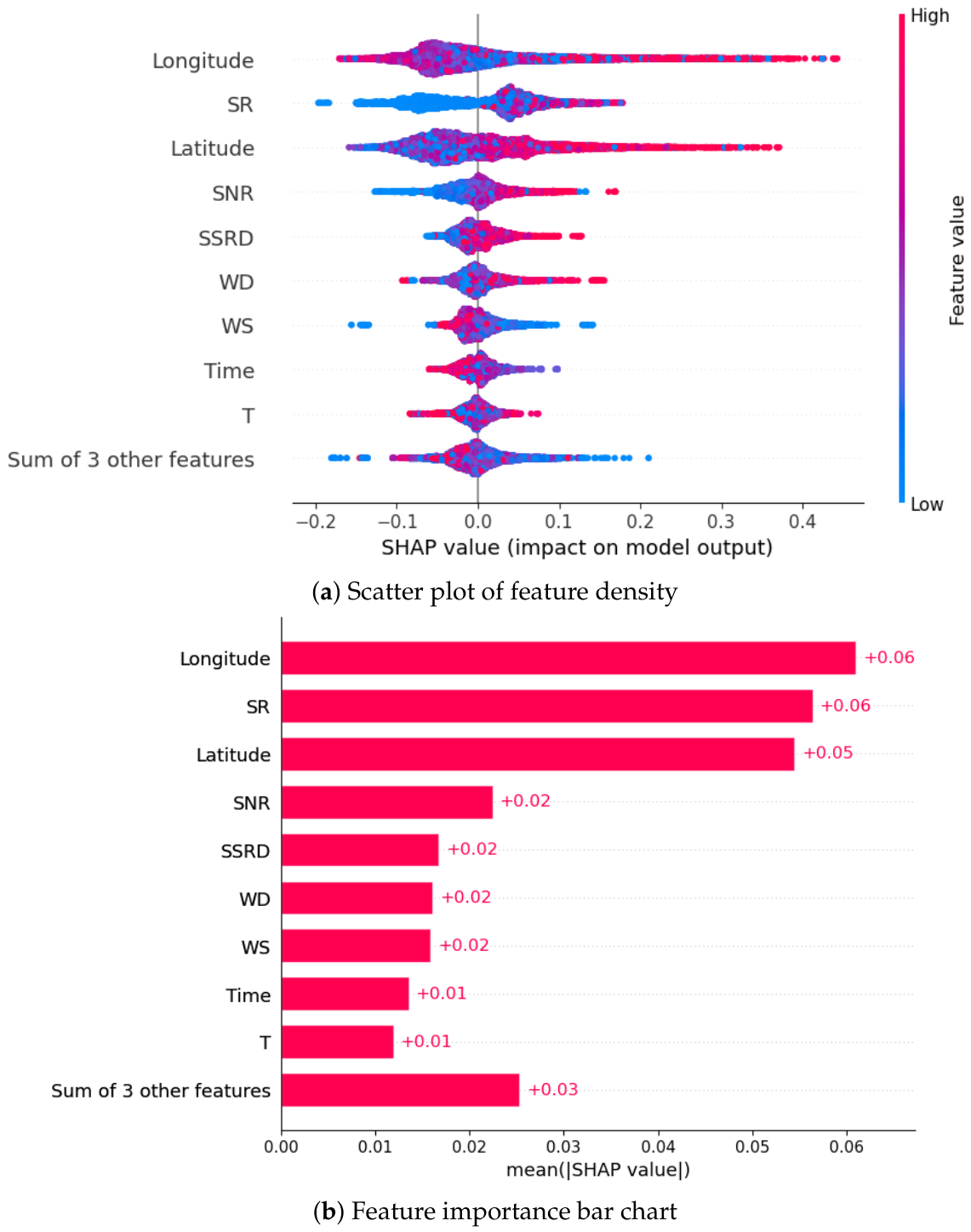
Figure 2 presents the SHAP analysis for the full-feature model. Figure 2a shows the distribution of SHAP values for each feature across all samples, highlighting how individual feature values contribute to the predicted NDVI, while Figure 2b summarizes the mean absolute SHAP values and the overall importance of each predictor.

Latitude and longitude exhibited the largest SHAP magnitudes, indicating that the fitted model strongly relied on geographic location to reproduce persistent within-lake NDVI patterns. In this context, geographic coordinates function as lake-specific location encodings rather than transferable physical predictors. Their high contribution suggests that persistent spatial structure within the studied lakes accounts for a substantial part of the model prediction.

Among the non-geographic predictors, GNSS-R surface reflectivity (SR) showed relatively large SHAP magnitudes, with higher SR values generally associated with positive contributions to the predicted NDVI. This relationship may reflect covariation among surface roughness, wind conditions, observation geometry, and surface bloom accumulation. Temperature and wind-related variables also contributed to the predictions: higher temperature values were generally associated with positive SHAP contributions, whereas stronger wind speed was often associated with negative contributions.

Overall, the SHAP results show how the fitted model used geographic, GNSS-R, and meteorological predictors to generate NDVI estimates. These results describe statistical associations within the fitted model. The dominant contribution of geographic coordinates indicates that the reconstructed patterns are primarily constrained within the studied lake domains. Therefore, the reported accuracy should mainly be interpreted as within-domain reconstruction and interpolation performance rather than evidence of direct transferability to other lakes. Further evaluation using cross-lake or spatially independent validation is required before applying the framework to unseen lake domains.

To assess whether the incremental contribution of GNSS-R varied with NDVI state or wind conditions, the matched samples from 2018 to 2024 were further examined by comparing the absolute prediction errors of the M+C and G+M+C models:

$$\Delta AE=|{\mathrm{NDVI}}_{\mathrm{M}+\mathrm{C}}-{\mathrm{NDVI}}_{\mathrm{ref}}|-|{\mathrm{NDVI}}_{\mathrm{G}+\mathrm{M}+\mathrm{C}}-{\mathrm{NDVI}}_{\mathrm{ref}}|.$$

(9)

Positive $\Delta AE$ values indicate a reduction in absolute prediction error associated with the inclusion of GNSS-R observations. The mean $\Delta AE$ remained close to zero across most NDVI and wind-speed intervals, although slightly larger positive values occurred at some intermediate-to-high NDVI levels. The error reduction did not show a clear dependence on wind speed (Figure S2).

3.3. NDVI Reconstruction Performance

The reported accuracy represents within-domain interpolation rather than independent spatial prediction. Following the dual-situation modeling strategy introduced in Section 3.1, the G+M+C model was applied to GNSS-R-covered regions, while the M+C model was used in regions without GNSS-R coverage. The annual test results for Lake Taihu and Lake Chaohu from 2018 to 2024 are summarized in

Table 5. Annual NDVI prediction accuracy of the dual-situation CatBoost framework for Lake Taihu and Lake Chaohu.

Lake/Region	Year	Train ${\mathit{R}}^2$	Train RMSE	Val. ${\mathit{R}}^2$	Val. RMSE	Test ${\mathit{R}}^2$	Test RMSE
Taihu covered	2018	0.76	0.13	0.65	0.16	0.69	0.16
Taihu non-covered	2018	0.78	0.12	0.76	0.12	0.76	0.12
Taihu covered	2019	0.72	0.13	0.64	0.15	0.65	0.16
Taihu non-covered	2019	0.77	0.12	0.75	0.13	0.75	0.13
Taihu covered	2020	0.75	0.15	0.66	0.17	0.67	0.17
Taihu non-covered	2020	0.82	0.11	0.80	0.11	0.80	0.11
Taihu covered	2021	0.73	0.13	0.65	0.14	0.63	0.15
Taihu non-covered	2021	0.81	0.11	0.79	0.11	0.79	0.11
Taihu covered	2022	0.69	0.16	0.62	0.17	0.61	0.17
Taihu non-covered	2022	0.80	0.11	0.78	0.12	0.78	0.12
Taihu covered	2023	0.63	0.17	0.56	0.18	0.55	0.19
Taihu non-covered	2023	0.81	0.11	0.79	0.12	0.79	0.12
Taihu covered	2024	0.70	0.15	0.64	0.16	0.61	0.17
Taihu non-covered	2024	0.80	0.11	0.78	0.12	0.78	0.12
Chaohu covered	2018	0.74	0.13	0.66	0.12	0.78	0.11
Chaohu non-covered	2018	0.87	0.09	0.83	0.10	0.83	0.10
Chaohu covered	2019	0.74	0.14	0.66	0.15	0.68	0.15
Chaohu non-covered	2019	0.83	0.10	0.80	0.11	0.80	0.10
Chaohu covered	2020	0.67	0.12	0.57	0.14	0.56	0.14
Chaohu non-covered	2020	0.85	0.08	0.82	0.09	0.82	0.09
Chaohu covered	2021	0.74	0.11	0.66	0.13	0.63	0.14
Chaohu non-covered	2021	0.85	0.08	0.82	0.09	0.82	0.09
Chaohu covered	2022	0.78	0.10	0.66	0.13	0.64	0.14
Chaohu non-covered	2022	0.85	0.08	0.82	0.09	0.82	0.09
Chaohu covered	2023	0.63	0.13	0.57	0.13	0.56	0.15
Chaohu non-covered	2023	0.84	0.09	0.80	0.10	0.80	0.10
Chaohu covered	2024	0.73	0.13	0.61	0.15	0.58	0.16
Chaohu non-covered	2024	0.84	0.10	0.80	0.11	0.80	0.11

.

For Lake Taihu, GNSS-R-covered regions achieved test $R^2$ values ranging from 0.55 to 0.69, with a corresponding RMSE between 0.15 and 0.19. The highest performance occurred in 2018 (test $R^2$ = 0.69, RMSE = 0.16), while the lowest $R^2$ was observed in 2023. In non-GNSS-R-covered regions, test $R^2$ ranged from 0.75 to 0.80, with an RMSE between 0.11 and 0.13.

Similarly, for Lake Chaohu, GNSS-R-covered regions exhibited test $R^2$ values ranging from 0.56 to 0.78, with RMSE values between 0.11 and 0.16. The highest performance occurred in 2018, with a test $R^2$ of 0.78 and an RMSE of 0.11. non-GNSS-R-covered regions showed consistently higher test performance, with $R^2$ values between 0.80 and 0.83 and RMSE values ranging from 0.09 to 0.11. Compared with Lake Taihu, Lake Chaohu generally exhibited lower RMSE, particularly in non-GNSS-R-covered regions.

An additional week-grouped sensitivity analysis was conducted using the 2018–2024 datasets (see

Table 6. Performance of the week-grouped sensitivity analysis for Lake Taihu and Lake Chaohu using the 2018–2024 datasets.

Lake	Situation	Train ${\mathit{R}}^2$	Train RMSE	Val. ${\mathit{R}}^2$	Val. RMSE	Test ${\mathit{R}}^2$	Test RMSE
Taihu	GNSS-R-covered	0.71	0.14	0.20	0.23	0.32	0.25
Taihu	Non-GNSS-R-covered	0.74	0.13	0.48	0.18	0.49	0.18
Chaohu	GNSS-R-covered	0.82	0.10	0.33	0.17	0.29	0.20
Chaohu	Non-GNSS-R-covered	0.81	0.10	0.47	0.16	0.49	0.16

). For Lake Taihu, the test $R^2$ values were 0.32 and 0.49 for the GNSS-R-covered and non-GNSS-R-covered situations, respectively, with corresponding RMSE values of 0.25 and 0.18. For Lake Chaohu, the corresponding $R^2$ values were 0.29 and 0.49, with RMSE values of 0.20 and 0.16. The lower performance obtained when complete weekly groups were separated among the training, validation, and test subsets suggests that temporal dependence may partly account for the higher accuracy observed under random sample splitting.

The GNSS-R-covered and non-GNSS-R-covered results in Table 5 are not directly comparable because they are based on different sample sets and predictor combinations. The contribution of GNSS-R was therefore examined using the ablation results in Table 4, where the different predictor combinations were evaluated on the same GNSS-R-matched samples.

GNSS-R remains observable under cloudy and low-illumination conditions and provides a microwave measurement of the lake surface. ERA5-Land variables describe environmental forcing, while geographic coordinates encode spatial location. In the present framework, the G+M+C model is therefore applied where GNSS-R observations are available, while the M+C model is used to complete the remaining lake area and maintain spatial continuity.

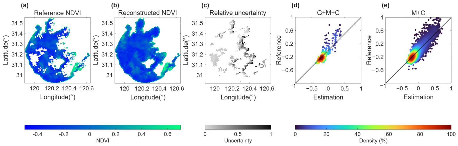
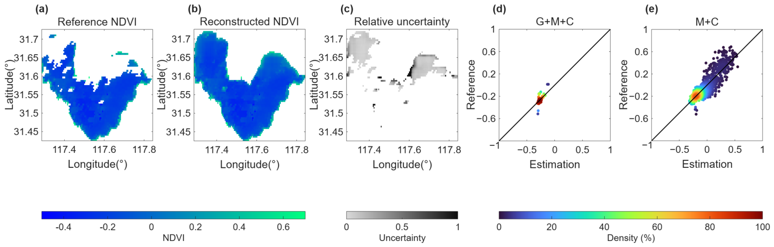
Figure 3 and Figure 4 show representative NDVI reconstruction results and corresponding relative uncertainty maps for Lake Taihu and Lake Chaohu. In the illustrated cases, the reconstructed NDVI fields reproduced several broad spatial patterns visible in the available MODIS reference images and filled areas affected by cloud contamination or incomplete optical observations. Lower relative uncertainty was observed over much of the open-water area, whereas locally higher values occurred near some shorelines and complex water–land boundaries. These values represent relative model-derived uncertainty within the corresponding lake-year dataset rather than absolute error probabilities. The scatterplots show predicted NDVI versus valid MODIS reference NDVI for the corresponding modeling situations rather than validation of optically missing pixels on the illustrated date.

4. Discussion

4.1. Cross-Product Spatial Consistency Comparison with FY-3F NDVI

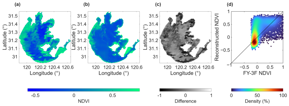
To examine the broad spatial consistency of the reconstructed NDVI, a cross-product comparison was conducted with FY-3F NDVI products. The FY-3F product has a coarser spatial and temporal resolution (1000 m, 10 day) than the reconstructed NDVI generated in this study (500 m, daily). Therefore, this comparison was used as an external spatial consistency check rather than as a strict pixel-level accuracy validation.

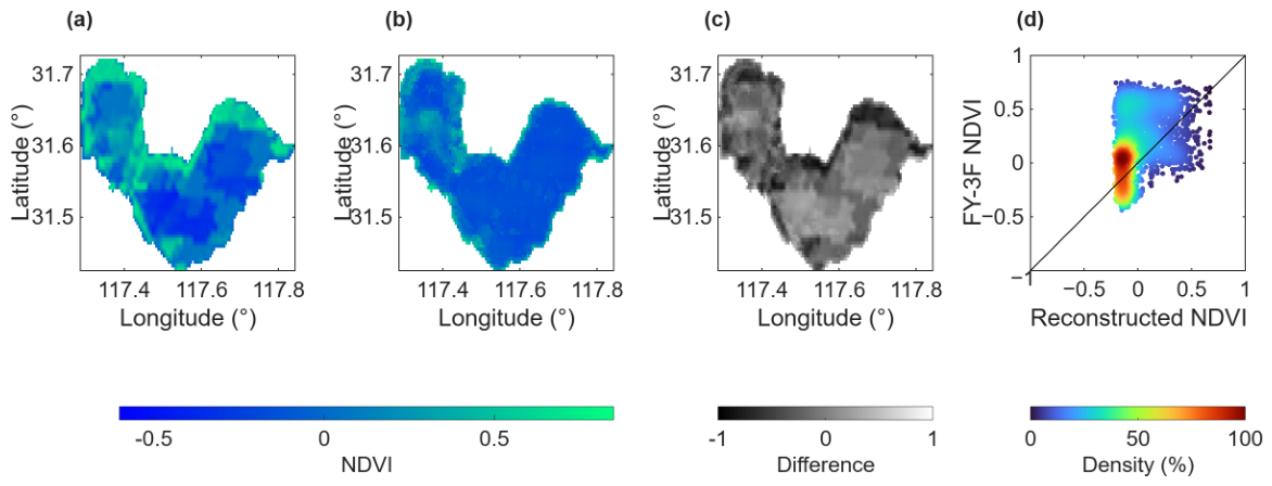
After resampling FY-3F NDVI to the MODIS grid, the reconstructed and FY-3F products showed broad agreement in several central open-water spatial patterns in Lake Taihu and Lake Chaohu (Figure 5 and Figure 6). In particular, several high-NDVI patches and large-scale spatial gradients occurred in similar locations in the two products.

Differences were more evident near shorelines and complex water–land boundaries. In these areas, FY-3F generally showed higher NDVI values in some pixels, whereas the reconstructed product appeared spatially smoother. These discrepancies may reflect differences in spatial resolution, temporal compositing, land contamination, mixed pixels, resampling, and model smoothing. Greater spatial smoothness should not be interpreted as evidence of greater physical accuracy.

In the illustrated comparisons, the reconstructed NDVI was approximately 0.1 lower than FY-3F on average. This difference is non-negligible but should not be interpreted solely as a systematic bias of the reconstructed product. Differences in spatial resolution, temporal compositing, sensor characteristics, resampling, and mixed-pixel effects near lake boundaries may all contribute to the observed offset. No bias correction was applied because FY-3F was used as an independent cross-product reference rather than as a calibration target. The reconstructed product nevertheless reproduced several broad spatial gradients and high-NDVI patches observed in FY-3F, particularly in central open-water regions.

Overall, FY-3F provides a useful external reference for examining broad spatial patterns, with the largest discrepancies occurring near lake boundaries.

The ablation results showed that geographic and meteorological predictors explained a large proportion of the predictable NDVI variability, while the incremental contribution of GNSS-R was modest. Previous studies have nevertheless demonstrated the potential of GNSS-R for sensing lake-surface conditions. For example, Zhang et al. [25] reported that the performance of spaceborne GNSS-R for algal-bloom detection in Lake Taihu varied with wind conditions. To examine whether a stronger GNSS-R contribution occurred under specific conditions, the absolute prediction errors of the M+C and G+M+C models were compared across reference-NDVI and wind-speed intervals using the matched samples from 2018 to 2024. The resulting error reduction remained modest across most intervals, although slightly larger reductions occurred at some intermediate-to-high NDVI values, while no clear dependence on wind speed was evident. In this study, GNSS-R was evaluated within a lake-wide daily reconstruction framework, where uneven CYGNSS sampling, observation geometry, spatial heterogeneity, meteorological variability, and shoreline mixed-pixel effects are all relevant to the observed model performance. The results therefore suggest that GNSS-R provides supplementary information in the present reconstruction framework.

4.2. Interannual Variation in Lake-Surface NDVI Signals

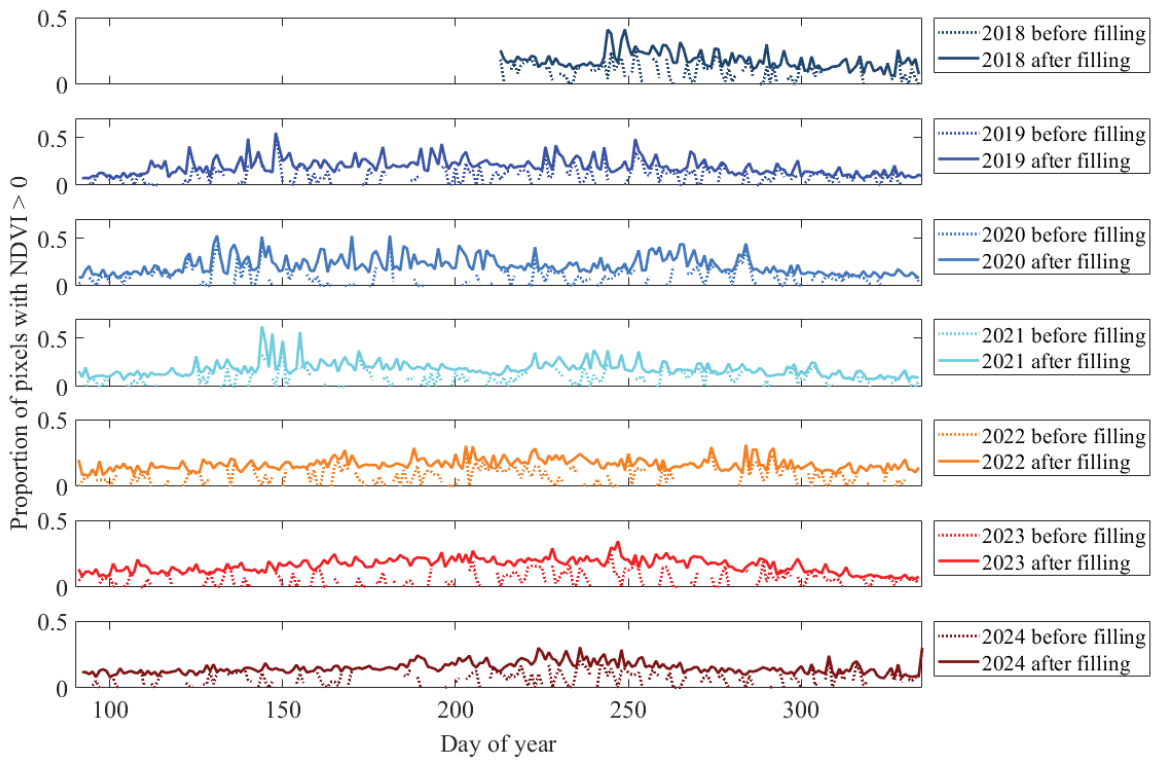
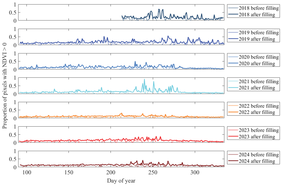
For each day, the proportion of positive-NDVI pixels was calculated as

$$P_t={\displaystyle \frac{N_t(\mathrm{NDVI}>0)}{N_{\mathrm{lake}}}},$$

(10)

where $N_t(\mathrm{NDVI}>0)$ is the number of pixels with NDVI greater than zero on day t, and $N_{\mathrm{lake}}$ is the fixed total number of pixels within the corresponding lake mask. Previous studies have used different NDVI thresholds for cyanobacterial bloom identification in Lake Taihu, including approximately −0.02, −0.012, and 0.05 for different sensors and applications [24,31,32]. In this study, NDVI > 0 was used to separate positive lake-surface NDVI signals from the background water signal for interannual comparison, rather than as a general threshold for cyanobacterial bloom detection.

The same lake-mask denominator was used before and after reconstruction under missing optical observations. Before reconstruction under missing optical observations, pixels with missing NDVI remained part of the fixed denominator but were not counted in the numerator.

The interannual NDVI line charts (Figure 7 and Figure 8) show that both Lake Taihu and Lake Chaohu exhibited frequent high-NDVI lake-surface signals during 2018–2021, with elevated peak values and closely spaced seasonal peaks mainly occurring in summer and autumn. These high-NDVI signals are generally consistent with periods of enhanced surface algal accumulation, but they should not be interpreted as direct quantitative measurements of cyanobacterial biomass. From 2022 onward, the NDVI peaks generally decreased and the fluctuations became milder, suggesting a reduction in high-NDVI surface accumulation signals or changes in lake-surface ecological conditions. It should be noted that the NDVI analysis was conducted at the whole-lake scale, and the eastern vegetation-dominated region of Lake Taihu was not separately masked. Therefore, the reconstructed NDVI includes not only cyanobacterial surface accumulation signals but also possible contributions from aquatic vegetation and mixed shoreline pixels. This limitation introduces uncertainty when interpreting interannual NDVI variations purely as changes in cyanobacterial bloom dynamics.

The observed decrease after 2022 may be related to a combination of environmental variability and strengthened watershed management. Seasonal and interannual changes in temperature, solar radiation, wind conditions, and hydrodynamic processes can directly influence cyanobacterial growth, surface aggregation, and the expression of positive-NDVI signals. At the same time, pollution control, ecological restoration, cyanobacteria harvesting, dredging, and aquatic vegetation restoration implemented in the Taihu and Chaohu basins may also have contributed to changes in lake-surface ecological conditions.

However, these factors were not quantitatively separated in this study. Therefore, the discussion of watershed management and engineering measures is intended only to provide contextual information for interpreting the observed NDVI changes, rather than direct causal evidence. A formal attribution analysis would require additional water-quality, hydrodynamic, meteorological, and management datasets.

Overall, the reconstructed daily NDVI captures both short-term seasonal fluctuations and longer-term interannual changes in lake-surface ecological signals, providing a spatially continuous and temporally dense dataset. Because NDVI is an integrated optical indicator affected by surface algal accumulation, aquatic vegetation, mixed pixels, and hydrometeorological conditions, the interannual results should not be interpreted as a direct measure of cyanobacterial bloom intensity. Instead, they provide a useful basis for further analyses of bloom-related surface dynamics, ecological responses, and potential driving factors over multiple years.

4.3. Ecological Consistency Check Using In Situ Observations in Lake Taihu

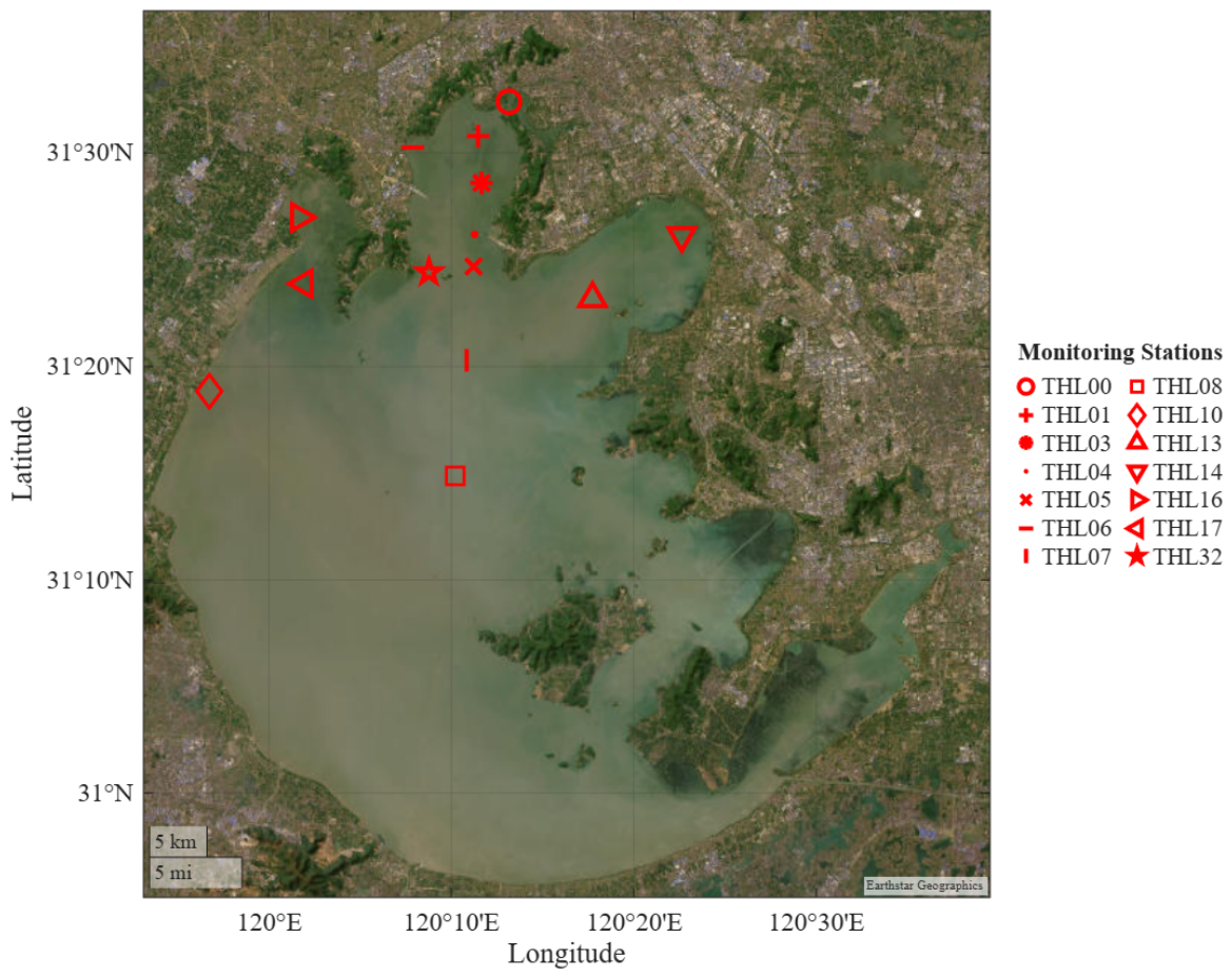
To examine whether the reconstructed NDVI retained ecologically meaningful bloom-related information, water-quality observations from Taihu monitoring stations were compared with the corresponding NDVI time series. Figure 9 shows the spatial distribution of the 14 monitoring stations in Lake Taihu. Because the in situ observations were collected quarterly from 2018 to 2020, whereas the reconstructed NDVI was generated daily, the comparison was used mainly as an ecological consistency check rather than as strict day-to-day or pixel-level validation.

For each monitoring station, the corresponding NDVI value was calculated as the mean of the valid pixels within a $3\times 3$ neighborhood centered on the 500 m grid cell containing the station coordinate. Invalid or missing pixels within the neighborhood were excluded from the calculation. The resulting neighborhood-averaged NDVI was then matched to the corresponding in situ sampling date. This neighborhood-based extraction was used to reduce the influence of isolated pixel noise, small geolocation differences, and spatial mismatch between point-based field observations and gridded satellite data.

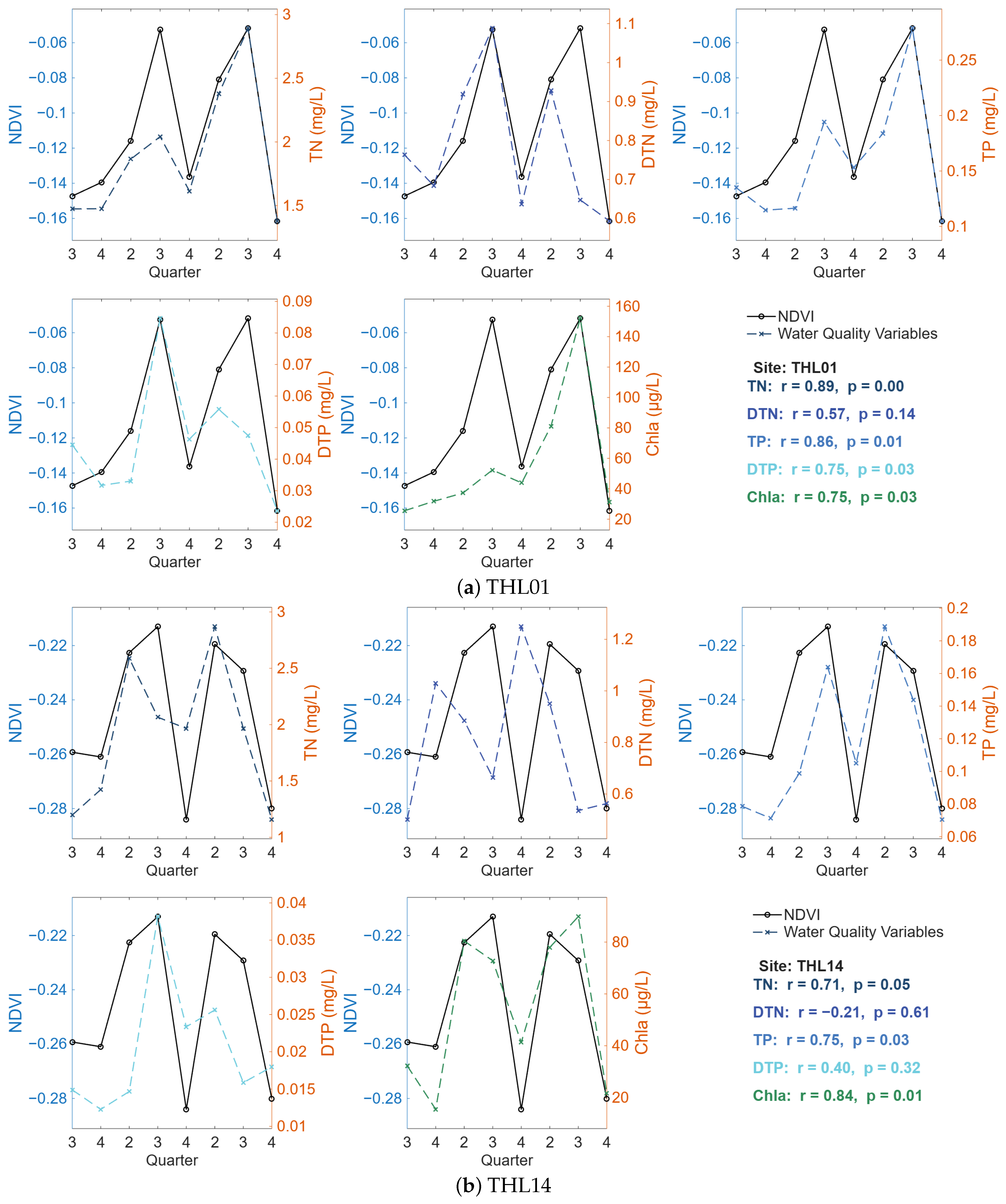
Correlations between reconstructed NDVI and the in situ indicators varied among the 14 monitoring stations (Table S1). For chlorophyll-a (Chl-a), significant positive correlations ($p<0.05$) were observed at THL01, THL13, THL14, and THL16, with r values ranging from 0.75 to 0.87, whereas the remaining stations showed weaker or statistically insignificant relationships. THL01 and THL14 are retained in Figure 10 as illustrative examples because they showed relatively clearer correspondence with reconstructed NDVI.

This variability is expected because station-based water-quality measurements represent local water-column conditions at discrete sampling times, whereas NDVI mainly reflects surface or near-surface optical signals over a spatial neighborhood. Although the $3\times 3$ neighborhood averaging reduces isolated pixel noise and small geolocation mismatches, it represents a nominal area of approximately $1.5\mathrm{km}\times 1.5\mathrm{km}$ and therefore cannot fully reproduce the local conditions measured at an individual station. In addition, local hydrodynamics, wind-driven transport, shoreline mixing, aquatic vegetation, water–land mixed pixels, and temporal mismatch between satellite observations and field sampling may weaken the correspondence between NDVI and in situ indicators.

As shown in Figure 10, the neighborhood-averaged NDVI series at THL01 and THL14 showed relatively clear temporal correspondence with chlorophyll-a (Chl-a), with correlation coefficients of 0.75 and 0.84, respectively (both $p<0.05$). These correlations provide supporting evidence that the reconstructed NDVI retained bloom-related ecological information under favorable station and sampling conditions.

This correspondence is physically plausible because Chl-a is closely related to phytoplankton biomass, whereas NDVI reflects the optical response of surface or near-surface materials. When phytoplankton biomass increases and cyanobacteria accumulate near the water surface, the water body may exhibit a stronger vegetation-like spectral response, potentially resulting in higher NDVI values. However, the correlations observed at THL01 and THL14 should not be interpreted as direct validation of all reconstructed NDVI values because the field observations were temporally sparse and spatially local, and only two favorable stations were selected for detailed illustration.

The relationships between NDVI and nutrient indicators were more variable. At THL01, NDVI showed comparatively high correlations with total nitrogen (TN), total phosphorus (TP), and dissolved total phosphorus (DTP), suggesting that nutrient variation and lake-surface optical signals were relatively synchronized at this station. At THL14, NDVI corresponded more clearly with TN and TP, whereas its relationships with dissolved total nitrogen (DTN) and DTP were weaker. These differences indicate that nutrient concentrations and lake-surface optical signals did not always vary synchronously.

This pattern is consistent with the eutrophication process in shallow lakes. Nitrogen and phosphorus provide important nutrient conditions for phytoplankton growth, and excessive nutrient loading may promote algal growth, including cyanobacterial blooms [33]. However, the transition from nutrient enrichment to observable surface algal accumulation is affected by several intermediate processes, including biological growth, vertical mixing, wind-driven transport, temperature, solar radiation, and local hydrodynamic conditions. Consequently, the neighborhood-averaged NDVI would not be expected to show equally strong relationships with all nutrient forms or at all monitoring stations.

Compared with nutrient indicators, Chl-a showed a more direct correspondence with the reconstructed NDVI at the two selected stations because Chl-a is more closely related to algal biomass. Overall, the station-based comparison provides supporting evidence that the reconstructed NDVI retained bloom-related ecological information under favorable station and sampling conditions.

5. Conclusions

This study developed a lake-specific multi-source machine learning framework for reconstructing missing daily lake-surface NDVI by integrating CYGNSS observations, ERA5-Land meteorological variables, geographic coordinates, and CatBoost. The framework was designed for within-lake NDVI reconstruction under incomplete optical observations rather than for direct GNSS-R retrieval of optical NDVI. It was applied to Lake Taihu and Lake Chaohu to generate spatially continuous daily NDVI fields from 2018 to 2024.

The ablation analysis showed that meteorological variables and geographic coordinates accounted for most of the predictable NDVI variation. On the same GNSS-R-matched sample domain, the G+M+C model achieved an average test $R^2$ of 0.63 and an RMSE of 0.15, compared with an $R^2$ of 0.62 and an RMSE of 0.16 for the M+C model. Thus, the inclusion of GNSS-R observables provided a modest supplementary contribution rather than a dominant improvement. In regions without GNSS-R observations, the M+C model was used to maintain lake-wide spatial continuity.

SHAP analysis showed that the fitted models relied strongly on geographic coordinates, while GNSS-R surface reflectivity, temperature, and wind-related variables also contributed to the predictions. Geographic coordinates acted primarily as lake-specific location encodings that helped reproduce persistent within-lake spatial patterns. The statistical associations between GNSS-R observables and predicted NDVI reflect model behavior rather than a direct physical relationship between microwave scattering and optical NDVI.

The comparison with FY-3F NDVI showed broad cross-product spatial consistency in several central open-water regions, while differences near shorelines were influenced by spatial-resolution differences, temporal compositing, mixed pixels, land contamination, and resampling. The station-based comparison at THL01 and THL14 showed relatively clear correspondence between the neighborhood-averaged NDVI series and Chl-a under favorable station and sampling conditions. However, the sparse quarterly observations and spatial-scale differences prevent comprehensive validation of the final reconstructed NDVI product.

The final reconstructed NDVI series showed seasonal and interannual variations in high-NDVI lake-surface signals. Both lakes exhibited relatively frequent and pronounced positive-NDVI signals during 2018–2021, whereas the magnitude and frequency of these signals generally decreased after 2022. These variations may reflect the combined influence of meteorological variability, hydrodynamic conditions, ecological changes, and watershed-management activities. However, the NDVI series alone does not support causal attribution to any individual factor. In addition, because the analysis was conducted at the whole-lake scale, the reconstructed NDVI includes possible contributions from surface algal accumulation, aquatic vegetation, shoreline mixed pixels, and other lake-surface optical conditions. Therefore, it should not be interpreted as a direct quantitative measure of cyanobacterial biomass or bloom intensity.

Several limitations should be emphasized. First, the statistical association between GNSS-R observables and NDVI is indirect and condition-dependent. Second, the strong dependence on geographic coordinates improves within-lake interpolation but limits direct transfer of the trained models to unseen lakes or locations outside the training domain. Third, the week-grouped sensitivity analysis showed that model performance decreased when complete weekly groups were separated among the training, validation, and test subsets, suggesting that the higher accuracy obtained under random sample splitting is partly associated with temporal similarity among observations. Accordingly, the random-split results are best interpreted as within-domain reconstruction performance rather than independent temporal extrapolation capability. Fourth, the sparse and irregular distribution of CYGNSS specular points limits the proportion of lake pixels directly assisted by GNSS-R. Fifth, shoreline areas and vegetation-affected regions remain susceptible to mixed-pixel effects and land contamination. Finally, the FY-3F and in situ comparisons provide supporting consistency evidence rather than strict reconstruction validation.

Overall, the proposed framework provides a lake-specific empirical approach for generating spatially continuous daily NDVI fields under incomplete optical observation conditions. Future work should improve the treatment of shoreline and vegetation-affected areas, incorporate additional GNSS-R observations, evaluate the framework across lakes with different sizes, morphologies, and hydrodynamic conditions, and adopt spatially blocked, temporally blocked, and cross-lake validation strategies to assess transferability and extrapolation performance more rigorously.

References

1. Dudgeon, D.; Arthington, A.H.; Gessner, M.O.; Kawabata, Z.I.; Knowler, D.J.; Lévêque, C.; Naiman, R.J.; Prieur-Richard, A.H.; Soto, D.; Stiassny, M.L.J.; et al. Freshwater biodiversity: Importance, threats, status and conservation challenges. Biol. Rev. 2006, 81, 163–182. [Google Scholar] [CrossRef] [Scilit] [PubMed]
2. Holgerson, M.A.; Raymond, P.A. Large contribution to inland water CO2 and CH4 emissions from very small ponds. Nat. Geosci. 2016, 9, 222–226. [Google Scholar] [CrossRef] [Scilit]
3. Qin, B.; Zhu, G.; Gao, G.; Zhang, Y.; Li, W.; Paerl, H.W.; Carmichael, W.W. A Drinking Water Crisis in Lake Taihu, China: Linkage to Climatic Variability and Lake Management. Environ. Manag. 2010, 45, 105–112. [Google Scholar] [CrossRef] [Scilit] [PubMed]
4. Zhang, G.; Gu, X.; Zhao, T.; Zhang, Y.; Xu, L. Ecological and environmental changes and protection measures of lakes in China. Bull. Chin. Acad. Sci. (Chin. Version) 2023, 38, 358–364. [Google Scholar] [CrossRef]
5. Hallegraeff, G.; Bolch, C. Unprecedented toxic algal blooms impact on Tasmanian seafood industry. Microbiol. Aust. 2016, 37, 143–144. [Google Scholar] [CrossRef] [Scilit]
6. Fleming, L.E.; Kirkpatrick, B.; Backer, L.C.; Walsh, C.J.; Nierenberg, K.; Clark, J.; Reich, A.; Hollenbeck, J.; Benson, J.; Cheng, Y.S. Review of Florida red tide and human health effects. Harmful Algae 2011, 10, 224–233. [Google Scholar] [CrossRef] [Scilit] [PubMed]
7. Richlen, M.L.; Morton, S.L.; Jamali, E.A.; Rajan, A.; Anderson, D.M. The catastrophic 2008–2009 red tide in the Arabian gulf region, with observations on the identification and phylogeny of the fish-killing dinoflagellate Cochlodinium polykrikoides. Harmful Algae 2010, 9, 163–172. [Google Scholar] [CrossRef] [Scilit]
8. Dai, Y.; Yang, S.; Zhao, D.; Hu, C.; Xu, W.; Anderson, D.M.; Li, Y.; Song, X.P.; Boyce, D.G.; Gibson, L.; et al. Coastal phytoplankton blooms expand and intensify in the 21st century. Nature 2023, 615, 280–284. [Google Scholar] [CrossRef] [Scilit] [PubMed]
9. Shen, L.; Xu, H.; Guo, X. Satellite remote sensing of harmful algal blooms (HABs) and a potential synthesized framework. Sensors 2012, 12, 7778–7803. [Google Scholar] [CrossRef] [Scilit] [PubMed]
10. Zeng, J.; Yin, B.; Wang, Y.; Huai, B. Significantly decreasing harmful algal blooms in China seas in the early 21st century. Mar. Pollut. Bull. 2019, 139, 270–274. [Google Scholar] [CrossRef] [Scilit] [PubMed]
11. Huang, C.; Li, Y.; Yang, H.; Sun, D.; Yu, Z.; Zhang, Z.; Chen, X.; Xu, L. Detection of algal bloom and factors influencing its formation in Taihu Lake from 2000 to 2011 by MODIS. Environ. Earth Sci. 2014, 71, 3705–3714. [Google Scholar] [CrossRef] [Scilit]
12. Hou, X.; Feng, L.; Dai, Y.; Hu, C.; Gibson, L.; Tang, J.; Lee, Z.; Wang, Y.; Cai, X.; Liu, J.; et al. Global mapping reveals increase in lacustrine algal blooms over the past decade. Nat. Geosci. 2022, 15, 130–134. [Google Scholar] [CrossRef] [Scilit]
13. Ebel, P.; Meraner, A.; Schmitt, M.; Zhu, X.X. Multisensor data fusion for cloud removal in global and all-season sentinel-2 imagery. IEEE Trans. Geosci. Remote Sens. 2021, 59, 5866–5878. [Google Scholar] [CrossRef] [Scilit]
14. Shen, H.; Li, X.; Cheng, Q.; Zeng, C.; Yang, G.; Li, H.; Zhang, L. Missing information reconstruction of remote sensing data: A technical review. IEEE Geosci. Remote Sens. Mag. 2015, 3, 61–85. [Google Scholar] [CrossRef] [Scilit]
15. Xu, M.; Jia, X.; Pickering, M.; Jia, S. Thin cloud removal from optical remote sensing images using the noise-adjusted principal components transform. ISPRS J. Photogramm. Remote Sens. 2019, 149, 215–225. [Google Scholar] [CrossRef] [Scilit]
16. Gao, G.; Gu, Y. Multitemporal Landsat missing data recovery based on tempo-spectral angle model. IEEE Trans. Geosci. Remote Sens. 2017, 55, 3656–3668. [Google Scholar] [CrossRef] [Scilit]
17. Zeng, C.; Shen, H.; Zhang, L. Recovering missing pixels for Landsat ETM+ SLC-off imagery using multi-temporal regression analysis and a regularization method. Remote Sens. Environ. 2013, 131, 182–194. [Google Scholar] [CrossRef] [Scilit]
18. Chen, J.; Zhu, X.; Vogelmann, J.E.; Gao, F.; Jin, S. A simple and effective method for filling gaps in Landsat ETM+ SLC-off images. Remote Sens. Environ. 2011, 115, 1053–1064. [Google Scholar] [CrossRef] [Scilit]
19. Li, X.; Wang, L.; Cheng, Q.; Wu, P.; Gan, W.; Fang, L. Cloud removal in remote sensing images using nonnegative matrix factorization and error correction. ISPRS J. Photogramm. Remote Sens. 2019, 148, 103–113. [Google Scholar] [CrossRef] [Scilit]
20. Yan, Q.; Huang, W.; Jin, S.; Jia, Y. Pan-tropical soil moisture mapping based on a three-layer model from CYGNSS GNSS-R data. Remote Sens. Environ. 2020, 247, 111944. [Google Scholar] [CrossRef] [Scilit]
21. Yan, Q.; Huang, W. Spaceborne GNSS-R sea ice detection using delay-Doppler maps: First results from the UK TechDemoSat-1 mission. IEEE J. Sel. Top. Appl. Earth Obs. Remote Sens. 2016, 9, 4795–4801. [Google Scholar] [CrossRef] [Scilit]
22. Chen, Y.; Yan, Q. Unlocking the potential of CYGNSS for pan-tropical inland water mapping through multi-source data and transformer. Int. J. Appl. Earth Obs. Geoinf. 2024, 133, 104122. [Google Scholar] [CrossRef] [Scilit]
23. Yan, Q.; Chen, Y.; Jin, S.; Liu, S.; Jia, Y.; Zhen, Y.; Chen, T.; Huang, W. Inland water mapping based on GA-LinkNet from CyGNSS data. IEEE Geosci. Remote Sens. Lett. 2023, 20, 1500305. [Google Scholar] [CrossRef] [Scilit]
24. Zhen, Y.; Yan, Q. Improving spaceborne GNSS-R algal bloom detection with meteorological data. Remote Sens. 2023, 15, 3122. [Google Scholar] [CrossRef] [Scilit]
25. Zhang, Y.; Wang, Y.; Zhou, S.; Meng, W.; Han, Y.; Yang, S. Analysis on feasibility of detecting water blooms in Taihu Lake with spaceborne GNSS-R. J. Beijing Univ. Aeronaut. Astronaut. 2024, 50, 695–705. [Google Scholar] [CrossRef]
26. Zhen, Y.; Yan, Q. Recovering NDVI over lake surfaces: Initial insights from CYGNSS data enhanced by ERA-5 inputs. Int. J. Appl. Earth Obs. Geoinf. 2024, 135, 104253. [Google Scholar] [CrossRef] [Scilit]
27. Yan, Q.; Huang, W. Sea ice sensing from GNSS-R data using convolutional neural networks. IEEE Geosci. Remote Sens. Lett. 2018, 15, 1510–1514. [Google Scholar] [CrossRef] [Scilit]
28. Meraner, A.; Ebel, P.; Zhu, X.X.; Schmitt, M. Cloud removal in Sentinel-2 imagery using a deep residual neural network and SAR-optical data fusion. ISPRS J. Photogramm. Remote Sens. 2020, 166, 333–346. [Google Scholar] [CrossRef] [Scilit] [PubMed]
29. Dorogush, A.V.; Ershov, V.; Gulin, A. CatBoost: Gradient boosting with categorical features support. arXiv 2018, arXiv:1810.11363. [Google Scholar] [CrossRef] [Scilit]
30. Prokhorenkova, L.; Gusev, G.; Vorobev, A.; Dorogush, A.V.; Gulin, A. CatBoost: Unbiased boosting with categorical features. Adv. Neural Inf. Process. Syst. 2018, 31, 6638–6648. [Google Scholar]
31. Hang, X.; Li, X.; Li, Y.; Zhu, S.; Li, S.; Han, X.; Sun, L. High-frequency observations of cyanobacterial blooms in Lake Taihu (China) from FY-4B/AGRI. Water 2023, 15, 2165. [Google Scholar] [CrossRef] [Scilit]
32. Li, X.; Hang, X.; Zhu, S.; Sun, L.; Li, Y. Response of cyanobacterial blooms to climate warming: Evidence from satellite observations and long-term trends in Lake Taihu in China. Sci. Rep. 2025, 15, 38820. [Google Scholar] [CrossRef] [Scilit] [PubMed]
33. Zhang, Y.; Li, M.; Dong, J.; Yang, H.; Van Zwieten, L.; Lu, H.; Alshameri, A.; Zhan, Z.; Chen, X.; Jiang, X.; et al. A critical review of methods for analyzing freshwater eutrophication. Water 2021, 13, 225. [Google Scholar] [CrossRef] [Scilit]
Figure 1. Lakes in the study area.
Remotesensing 18 03269 g001
Figure 2. SHAP-based feature importance analysis. T, temperature; WS, wind speed; WD, wind direction; SSRD, surface solar radiation downwards.
Remotesensing 18 03269 g002
Figure 3. Representative NDVI reconstruction results for Lake Taihu on 6 June 2021: (a) reference NDVI; (b) reconstructed NDVI; (c) relative uncertainty; (d) predicted-versus-reference scatterplot for the G+M+C model; and (e) predicted-versus-reference scatterplot for the M+C model. The solid black lines in (d,e) denote the 1:1 reference line.
Remotesensing 18 03269 g003
Figure 4. Representative NDVI reconstruction results for Lake Chaohu on 17 August 2018: (a) reference NDVI; (b) reconstructed NDVI; (c) relative uncertainty; (d) predicted-versus-reference scatterplot for the G+M+C model; and (e) predicted-versus-reference scatterplot for the M+C model. The solid black lines in (d,e) denote the 1:1 reference line.
Remotesensing 18 03269 g004
Figure 5. Cross-product comparison over Lake Taihu on 31 August 2024: (a) FY-3F NDVI; (b) reconstructed NDVI; (c) difference calculated as reconstructed NDVI minus FY-3F NDVI; and (d) density scatterplot for pixels with valid values in both products. The solid black line in (d) denotes the 1:1 reference line.
Remotesensing 18 03269 g005
Figure 6. Cross-product comparison over Lake Chaohu on 20 October 2024: (a) FY-3F NDVI; (b) reconstructed NDVI; (c) difference calculated as reconstructed NDVI minus FY-3F NDVI; and (d) density scatterplot for pixels with valid values in both products. The solid black line in (d) denotes the 1:1 reference line.
Remotesensing 18 03269 g006
Figure 7. Daily proportion of lake-mask pixels with NDVI > 0 before and after reconstruction under missing optical observations over Lake Taihu from 2018 to 2024.
Remotesensing 18 03269 g007
Figure 8. Daily proportion of lake-mask pixels with NDVI > 0 before and after reconstruction under missing optical observations over Lake Chaohu from 2018 to 2024.
Remotesensing 18 03269 g008
Figure 9. Spatial distribution of the 14 water-quality monitoring stations in Lake Taihu.
Remotesensing 18 03269 g009
Figure 10. Ecological consistency comparison between reconstructed NDVI and in situ water-quality indicators at (a) THL01 and (b) THL14 in Lake Taihu.
Remotesensing 18 03269 g010