1. Introduction
Three-dimensional point clouds used for the analysis of topographic changes have changed the way we assess and manage geohazards and have helped us to understand a variety of geomorphological processes due to their high level of detail and ease of data collection. In the hazard community, analysis of point cloud representations of topography have been used to study rock slope failures [
1,
2,
3,
4], large scale landslides [
5,
6,
7], changes in permafrost terrain [
8,
9] and have been applied for assessment and monitoring of geohazards along transportation corridors [
10,
11], for example. In the geosciences and geomorphology, studies utilizing point clouds have included the study of fault zone deformation [
12], mapping lithology [
13], quantification of surface change in complex debris flow and river topography [
14,
15], the study of mass balance in glaciers [
16] and the study of small-scale processes in arctic catchments [
17], to name a few. Studies involving point clouds have even extended to the civil engineering realm, where they have been used to identify methane gas build up through deformation monitoring of a landfill [
18] and monitoring deformation in civil structures [
19].
Point clouds collected from a Terrestrial Laser Scanner (TLS) can be collected efficiently with high accuracy and resolution and can be used to detect small-scale topographic changes [
9,
15,
20]. Compared to change detection with radar systems [
7], TLS monitoring has some notable advantages over radar techniques, including its portability, its economy of operation, its ability to detect deformation in directions oblique to the laser line of sight and its higher accuracy point clouds. In addition, data processing is not affected by sudden accelerations [
21,
22,
23,
24]. This makes TLS particularly advantageous for studying topographic changes in 3D over a variety of study sites in complex geomorphological settings.
Some studies have investigated methods that take advantage of the law of large numbers, using the redundant points available in TLS point clouds, in order to detect change at scales smaller than that possible using single point accuracy. This has been done by using 3D surface matching [
6], averaging point cloud differences along one dimension of movement [
20] and by averaging the position along the local point cloud surface normal,
i.e., the Multiscale Model to Model Cloud Comparison (M3C2) algorithm [
15].There are, however, limited studies taking full advantage of the 3D nature and high spatial and temporal resolution of TLS-derived point clouds in order to detect very small levels of signals in a noisy dataset. This is particularly important for detecting and monitoring the precursor phase of slope failures, the study of small-scale geomorphic processes, such as sediment flux and erosion [
25], and for monitoring small-scale changes in civil infrastructure.
A four-dimensional (4D) noise-filtering and calibration algorithm is presented, which takes full advantage of redundancy in high spatial and temporal resolution point clouds derived from TLS systems. The aim is to achieve similar or better differential accuracy than radar systems (mm to sub-mm), while maintaining the ability to detect change in any direction. The application of this method is intended for studies where a high temporal resolution of scanning is possible.
2. Theoretical Framework
The ability to detect change by comparing a series of point clouds is controlled by the point cloud accuracy, precision, survey design and terrain factors. In TLS surveys, this includes: the scanner target distance [
26], vegetation [
27], incidence angle [
28,
29,
30], surface reflectance [
31], surface roughness [
15], atmospheric conditions [
32], heterogeneity in point spacing [
33], alignment error [
6] and instrument specifications [
34]. Some of these factors contribute to the random Gaussian point-to-point noise (precision), and others contribute to a systematic error [
35]; these errors are the main controlling factor in the ability to detect a change signal and result in the definition of a minimum signal where change can be confidently detected, known as the level of detection (LoD). The LoD is usually represented by 1.96-times the standard deviation of the residual distribution found from comparing sequential point clouds where no change has occurred, representing the 95% confidence level [
20]. In addition, TLS equipment can sometimes produce systematic effects; such as horizontal lines in certain side-to-side scanning instruments or vertical lines in rotating mirror scanners. Although this error appears to be systematic when comparing subsequent point clouds, it could be considered random in large temporal sampling programs.
Random noise, typically resulting from instrumental error and surface roughness, can be reduced or filtered through averaging. This is useful when the signal-to-noise (or random error) ratio is less than one or, in other words, when the signal is below the standard error of the mean. It is important to note that there are two possible averaging approaches applied to point clouds; those involving the averaging of the point cloud position (such as M3C2 [
15] or creating an average mesh, mesh smoothing) and those involving the averaging of differences between point clouds [
20]. Both reduce the standard error in a noisy point cloud, but the former can cause unwanted artifacts in high roughness surfaces or around occluded points. For the development of the filtering algorithm presented herein, the averaging of point cloud differences is applied exclusively.
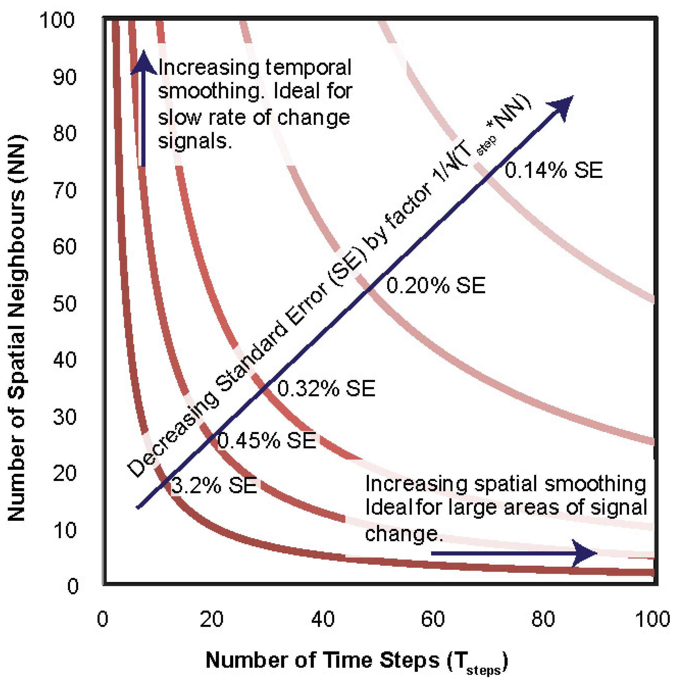
From an unknown population where repeated random samples are obtained, each with n observations, the sample means will follow a normal distribution, regardless of the distribution in which they are sampled. The average of the sample means approximates the population mean and improves with increasing numbers of n samples. The standard deviation of the samples’ means is known as the standard error and is σ/√n for n samples, where σ is the population standard deviation. The reduction in standard error as a result of averaging n samples is thus 1/√n (
Figure 1). For point clouds, this equates to averaging differences of a point either in the spatial or temporal domains. Averaging in the spatial domain can cause smoothing of a change signal; this is especially noticeable along the signal boundaries. A high degree of spatial averaging can be advantageous if the expected spatial extent of the signal is much larger than the radius of the neighbouring points used for averaging. Alternatively, averaging along the temporal domain can be applied; for example, in situations where continuous monitoring of terrain is warranted. As long as the temporal averaging window is much smaller than the expected rate of change, noise can be effectively reduced without smoothing the temporal trend. Practically, there is an optimum combination of spatial and temporal neighbours for a given signal being studied and for operational and budget constraints.
The combination of both spatial and temporal averaging has a great advantage over using either one on its own. By including neighbours both in space and time, an increase in the amount of neighbours for averaging can be obtained by multiplying the number of spatial neighbours by the considered time interval (T
step) (
Figure 1). For example, averaging 100 spatial neighbours over a time step of 10 point clouds results in a reduction in the standard error of approximately 32 times. This increases the potential of identifying signal changes from data with very small signal-to-noise ratios.
In terrain studies, a perfect Gaussian distribution of error cannot be expected. The complex nature of the rocky terrain being studied, as well as the presence of vegetation, can cause outliers to occur. To minimize the effect of these outliers, the median can be used for averaging instead of the mean. The median is robust against outliers and will result in values closer to the true signal, as demonstrated in 2D image enhancement (e.g., [
36]).
Figure 1.
Theoretical reduction in the standard error (SE) of sample means using combinations of spatial neighbours and time steps. The reduction in standard error is calculated using 1/√(Tstep*NN), where NN is the number of spatial neighbours and Tstep is the number of samples over time.
Figure 1.
Theoretical reduction in the standard error (SE) of sample means using combinations of spatial neighbours and time steps. The reduction in standard error is calculated using 1/√(Tstep*NN), where NN is the number of spatial neighbours and Tstep is the number of samples over time.
Systematic errors can be difficult to analyze and cannot be eliminated with statistical techniques, such as averaging. Repeated measurements will have no effect on the systematic error. Effective survey design and equipment maintenance can reduce systematic errors; for example by regular calibration of LiDAR equipment and designing surveys to reduce occlusion bias. However, these errors can seldom be eliminated by survey design alone. An effective way to remove systematic error in point clouds can be through self calibration [
35], the performance of the measurement on a known reference value and adjusting the procedure until the desired result is obtained. For point clouds of terrain, this can be achieved by adjusting the differences between multi-temporal point clouds for a short time period where no change is assumed to have occurred, utilizing an empirical approach.
It has been shown that a point cloud comparison directed along a localized normal is beneficial for geomorphological studies [
9,
15]. The direction for distance calculation has traditionally been computed in one dimension for the ease of calculation [
4,
5,
20,
37]. In complex terrain, it is unreasonable to expect change to occur in a single dimension or along a common direction. An example of a complex rock slope is White Canyon, in Western Canada, where both movement of talus and rock slope deformation are occurring in multiple directions and the slope is geomorphologically complex [
11].
3. Methods: Approach and Synthetic Tests
3.1. 4D Filtering and Systematic Calibration Approach
The proposed approach is based on frequent to continuous data acquisitions in order to take advantage of point redundancy in the temporal domain. The approach is applied to pre-processed data; data that have been converted from polar to Cartesian coordinates, filtered to remove vegetation and co-registered to a reference acquisition. Pre-processing is commonly applied in point cloud software packages by manually filtering vegetation and using an application of the iterative closest point (ICP) algorithm [
38] for co-registration [
39]. This manual approach can be onerous in large temporal sampling programs. The use of iterative and morphological filters on waveform TLS can be a solution for vegetation filtering [
40] and could allow for full automation of the pre-processing step. In this study, non-vegetated targets were scanned exclusively, and an automated application of the ICP algorithm was applied via a custom macro within Polyworks [
41].
In the proposed approach, calibration is used to reduce the effect of all types of systematic errors, and a four-dimensional (4D) de-noising technique is used to reduce the effect of random noise; both typical in TLS-based surveys. The first data collected are used for all distance calculations and as a reference for co-registration and are referred to as the “reference point cloud”. Subsequent scans used for calibration are referred to as “calibration data point clouds” and point clouds used for change detection after the collection of calibration clouds as “data point clouds”.
The combined approach consists of the following general steps:
- (1)
Acquisition of reference point cloud
- (2)
Acquisition of calibration point clouds
- (3)
Co-registration with reference point cloud using ICP
- (4)
Calculation of distances between the reference point cloud and the calibration data point clouds along the local normal
- (5)
Averaging of reference to calibration data point cloud distances along the time domain with a time step equal to the number of calibration data point clouds
- (6)
Acquisition of data point clouds for change detection
- (7)
Co-registration of data point clouds
- (8)
Calculation of reference to point cloud distances along the reference local normal
- (9)
Averaging of point cloud differences using nearest neighbours in space and time
- (10)
Subtraction of the calibration calculated in Step 2 from each filtered reference to data point cloud distances
The distance calculation approach is similar to the M3C2 method [
15], where distances are calculated along a local normal; however, there are two main differences: (1) distances are calculated from a noisy reference to a data point cloud in one direction only; and (2) a calibration is used to remove the effect of systematic errors in the reference point cloud. The projection scale radius in this case is also kept to a minimum, around the size of the data point cloud point spacing, to minimize artifacts created by a large projection scale; such as in environments with variable roughness or a high degree of curvature. The de-noising algorithm can, however, be adapted to any point cloud difference calculation method,
i.e., mesh to point, point to point, mesh-to-mesh,
etc.The use of a noisy reference scan results in both a noisy distance calculation and an additional systematic error. This systematic error is a result of using the same reference dataset in each reference to data calculation and cannot be removed by averaging distances over time. The systematic error at each point in the reference thus contributes to the standard error. In the proposed approach, a set of point clouds collected at the same frequency as the desired filtering interval (Tstep), before the collection of data point clouds, is used to remove all systematic errors, whether caused by the noisy reference, incident angle, roughness, etc. This is done using an empirical approach, by performing the filtering algorithm on the collected calibration datasets along the time dimension only and then subtracting the distance from each filtered reference to dataset distance in the 4D filtering step. The filtering reduces the random noise in the calibration datasets with sufficient precision (based on having an equal time step for calibration as compared to the time step for reference to data comparison) to allow convergence on the systematic error for each reference point. The precision of the calibration file determines the maximum attainable reduction through filtering without losing spatial resolution. The calculated systematic error is unique to the reference scan being used and should be repeated whenever a new reference scan is utilized.
The algorithm can be run without a calibration dataset; however, this will limit the possible reduction in standard error. The de-noising algorithm will converge on the systematic error specific to the reference. Furthermore, if calibration is conducted, it should be limited to a time frame where no change is expected. Calibration should be repeated after significant changes have occurred or during regular intervals.
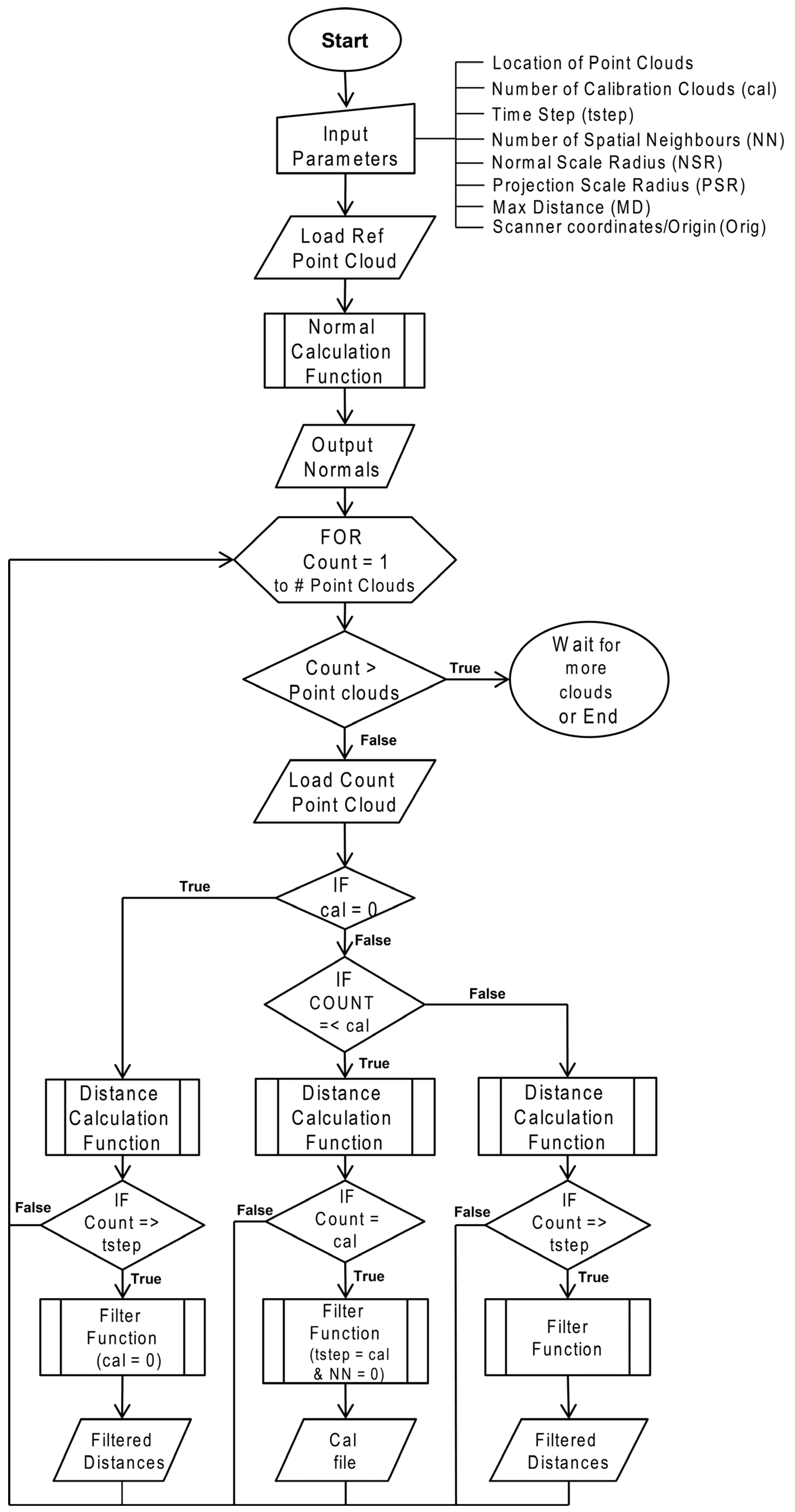
The algorithm structure is presented as a flow chart in
Figure 2. Subroutines of the main algorithm are presented as
supplementary material. For fast nearest neighbour searches, a binary tree data structure known as the k-d tree [
42] is used for efficient neighbourhood searches and is implemented in C++. A detailed description of the point cloud distance and 4D de-noising algorithm with incorporated calibration is provided in the following subsections.
3.1.1. Local Normal Calculation
The local surface normal of each point in the reference point cloud is calculated based on a user-defined selection of local points or search radius. The selection of local points depends on the point spacing, the roughness and geometry of the target of interest (see [
15]) and the projection scale. For rock slope studies, we are interested in calculating the local surface normal that is greater than the local surface roughness, but small enough to capture large-scale changes in slope morphology, between 0.5 and 10 m.
Figure 2.
Structured flow chart of the 4D filtering and calibration algorithm. Subroutines, the normal calculation function, the distance calculation function and filter function are presented as
supplementary material.
Figure 2.
Structured flow chart of the 4D filtering and calibration algorithm. Subroutines, the normal calculation function, the distance calculation function and filter function are presented as
supplementary material.
The calculation of local normal vectors results in two possible orientations, above or below the plane defined by the normal. For the purpose of setting a sign convention, all normals are oriented towards the local origin or any user-defined point. This is done by using the dot product of the normal with the ray from the origin to the normal vector position to determine its orientation. Negative dot product values are converted to positive, completing the change in orientation (see the
Supplementary Material, normal calculation algorithm). As a result, positive differences are related to movements towards the sensor (e.g., precursory deformation, accumulation), while negative differences represent rock slope failure source zones or depletion areas.
3.1.2. Point Cloud Difference Calculation
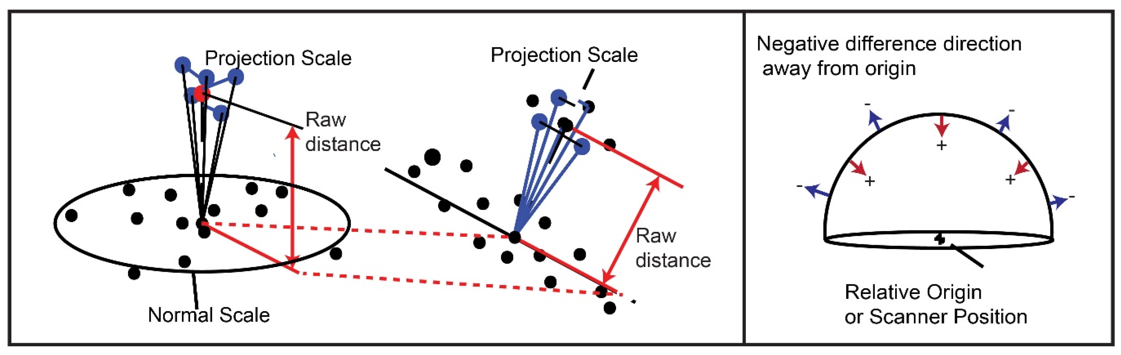
A nearest point region in the comparison point cloud (either calibration data or data) consisting of p points is calculated for each point in the reference point cloud (equivalent to the projection scale of M3C2). The mean distance from the reference point to the point region along the point normal is then calculated. This is done by projecting the vector distance from the point in the reference cloud to the data point in the local point region onto the normal vector (
Figure 2). The mean distance is then calculated. In very steep or highly changing terrain or with variable surface roughness, a high projection scale search radius will cause unwanted artifacts. This is typical for position averaging techniques. For this reason, a small number of points are used, no greater than the point spacing of the data cloud. The algorithm has an option to use the closest vector to the normal, which produces the best results in especially high surface roughness variation.
The distance is then used to find the coordinates of a new point in the data point cloud. The mean distance to a region of points in the reference cloud is then calculated and recorded as the raw point-to-point distance for the original reference query point. A difference direction is then assigned; differences in the same direction as the normal vector (towards the scanner) are positive, and differences in the opposite direction from the normal vector (away from the scanner) are negative (
Figure 3).
Figure 3.
Distance calculation method similar to the Multiscale Model to Model Comparison (M3C2) algorithm [
15]. (
Left) Distances are calculated along a local normal from the reference point to the mean location of a local point region. For high roughness point clouds, the projected closest vector to the normal distance can be used. (
Right) Difference vectors are assigned a sign convention, positive towards the scanner and negative away from the scanner.
3.1.3. 4D Filtering
The proposed four-dimensional de-noising technique filters the point differences in space and in a temporal dimension. Spatial neighbours are the closest point to a reference point, and temporal neighbours are the closest neighbours in space at a different time. It is important to note that the differences are being filtered exclusively; the geometrical position of the points in the clouds is not being changed as would be the case in smoothing a polygonal mesh. The filtering algorithm is based on the median, which is robust against outliers, such as vegetation or rogue reflections.
Starting from the first consecutive data point cloud (T
1) after the reference cloud (T
R) is added to the temporal filtering time step (T
step), (T
R + T
1 + T
step), filtered distances are calculated. Using a k-d tree-based nearest neighbour search algorithm [
42], spatial neighbours (number of spatial neighbours (NN)) are found for each point in T
R + T
1 + T
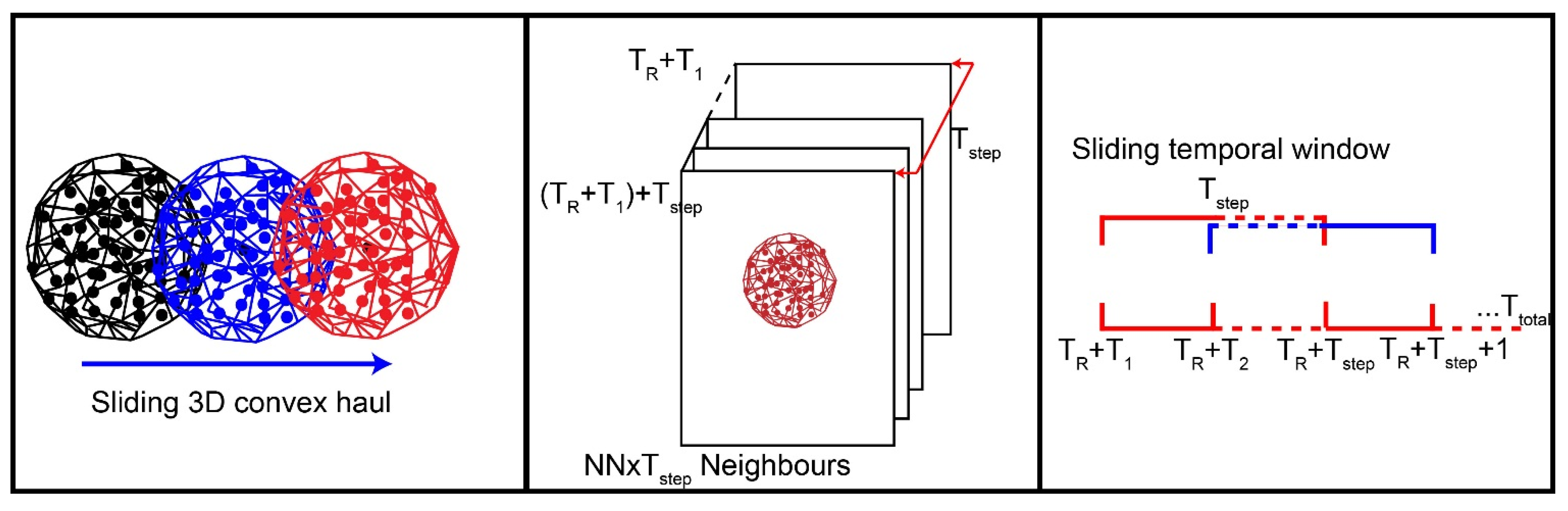
step. Since this is done for each point in the cloud, overlapping points are considered; this is equivalent to sliding a 3D convex haul consisting of NN through space (
Figure 4). For each nearest neighbour found, temporal neighbours are also found. This is done by finding the NN of each point in each point cloud considered in T
step. Once the NNxT
step neighbours are found for each point, the assigned difference values are filtered using the median. Compared to mean or averaging, median filtering preserves edges while removing noise efficiently [
36].
These steps are repeated for each consecutive point cloud (T2,T3…Ti); this is equivalent to sliding the temporal window of size Tstep through time.
Figure 4.
(Left) The search for spatial neighbours is equivalent to sliding a 3D convex haul containing NN through space for each point. Middle: the search for temporal neighbours is done for each point in the convex haul part of the considered time interval (Tstep). (Right) Starting from the first data point cloud (T1) after the reference (TR) over the considered time interval (Tstep), (TR + T1 + Tstep), the median values are calculated. This is repeated for each consecutive data point cloud (T2,T3…Ti), which is equivalent to sliding the temporal window of size Tstep through time.
3.2. Synthetic Tests and Parameter Selection
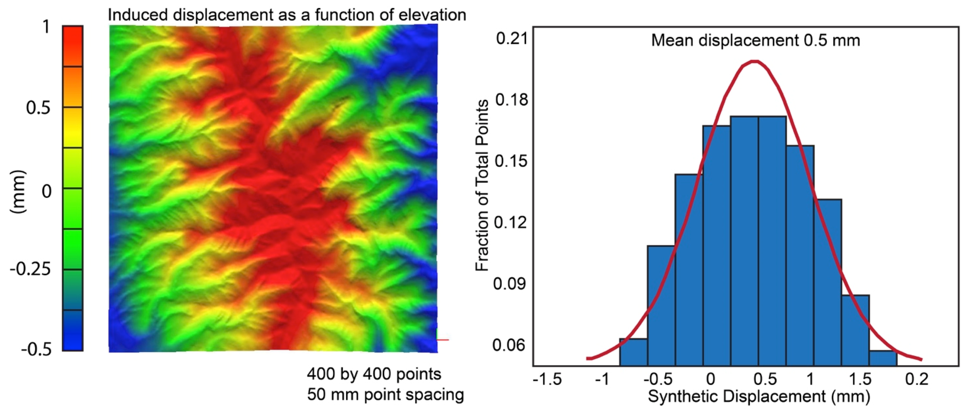
The development and testing of the algorithm was conducted using synthetic displacements induced on a real digital elevation model (
Figure 5). Synthetic displacements were added as a function of elevation (ΔZ) simulating terrain evolution. Negative displacements (loss) were induced for the highest elevations, and positive (accumulation) ones were induced for the lower elevations. The point cloud was constructed with 400 by 400 points in the horizontal plane, with a point spacing of 0.05 m or units. For most of the algorithm testing, a mean displacement of 0.5 mm was introduced. Gaussian noise was added to comparison point clouds with a standard deviation of 0.015 m or a mean signal-to-noise ratio of 0.033. This signal-to-noise ratio was chosen to highlight the capabilities of space and time noise filtering; current methods [
15,
20] are unable to separate a signal at this ratio. The effect of using both space and time neighbours was tested (
Section 3.2.1) and a practical combination of them (
Section 3.2.2) using a reference without noise. To test the optimum parameters for calibration, a reference point cloud with identical noise level as the data point clouds was used (
Section 3.2.3).
Figure 5.
(Left) True signal, with induced synthetic change between −0.0005 m and 0.001 m on the DEM as a function of height. (Right) Distribution of induced synthetic change with mean 0.0005 m displacement.
Figure 5.
(Left) True signal, with induced synthetic change between −0.0005 m and 0.001 m on the DEM as a function of height. (Right) Distribution of induced synthetic change with mean 0.0005 m displacement.
3.2.1. Effect of Space and Time Neighbours
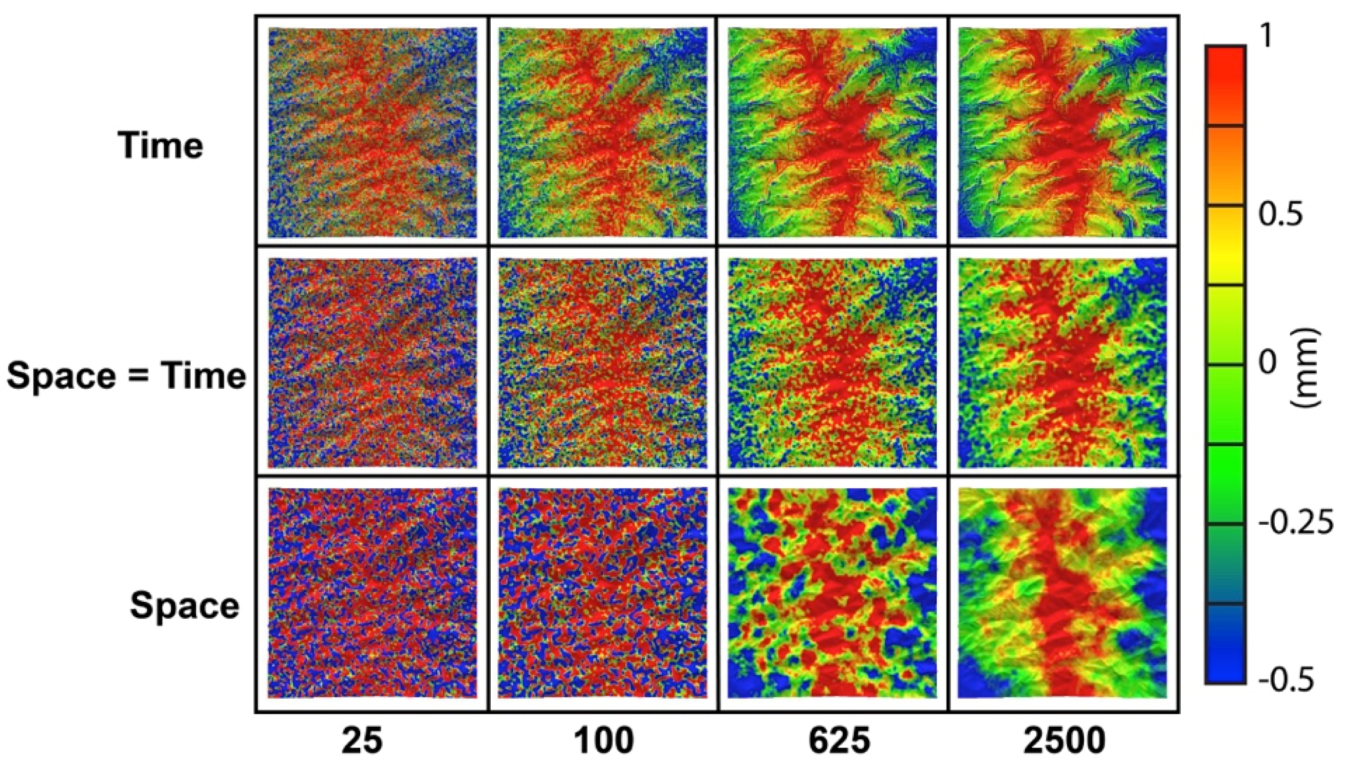
To test the effect of spatial and temporal filtering, the filtered results from 25 to 2500 neighbours were compared for space filtering alone, time filtering alone and a combination comprising equal space and time neighbours (
Figure 6). For each case, a reduction in standard deviation close to theoretical was observed, indicating the good performance of the algorithm. The time filtering alone case resulted in the best spatial resolution of the signal. Although using a constant number of neighbours with different combinations of space and time resulted in the same reduction in standard deviation, the ability to resolve the signal is affected solely by the spatial neighbours. For the space only case, loss in spatial resolution was indicated by spatial smoothing, clustering and a gradual coalescence of the signal. The space equal to time case provided a reasonable ability to resolve the signal with the benefit of having the square root of the total neighbours in each space and time domain; which is the most practical of the cases tested.
For both the time only filtering case and the space equal time filtering case, the ability to resolve the signal at the underlying signal-to-noise ratio was reasonable at 625 neighbours. The addition of the next filter level, 2500 neighbours, did not provide a significant increase in the ability to resolve the signal. Note that too much filtering (too many total neighbours) relative to the signal-to-noise ratio will not improve the ability to resolve the signal after a certain number of neighbours. At a certain point, when the noise is an order of magnitude or greater than the signal, the ability to resolve will not be significantly improved, just the precision of the distance measurement.
Figure 6.
Filtered synthetic DEM distances with a signal-to-noise ratio of 0.033 with time neighbours only (
upper row), with equal space and time neighbours (
middle row) and with space neighbours only (
lower row). The true signal is presented in
Figure 5, left inset.
Figure 6.
Filtered synthetic DEM distances with a signal-to-noise ratio of 0.033 with time neighbours only (
upper row), with equal space and time neighbours (
middle row) and with space neighbours only (
lower row). The true signal is presented in
Figure 5, left inset.
3.2.2. Selection of Optimum Neighbourhood
It is unlikely that a high degree of filtering in the temporal domain is practical even with high speed laser scanning. Some degree of spatial filtering can have a substantial impact on the level of detection; this is the result of the standard error reduction being proportional to the time step multiplied by the number of neighbours. The appropriate number of time steps and spatial neighbours will depend on the signal being studied, both in terms of its spatial extent and temporal rate of change, the resolution and on project constraints (time, budget, etc.).
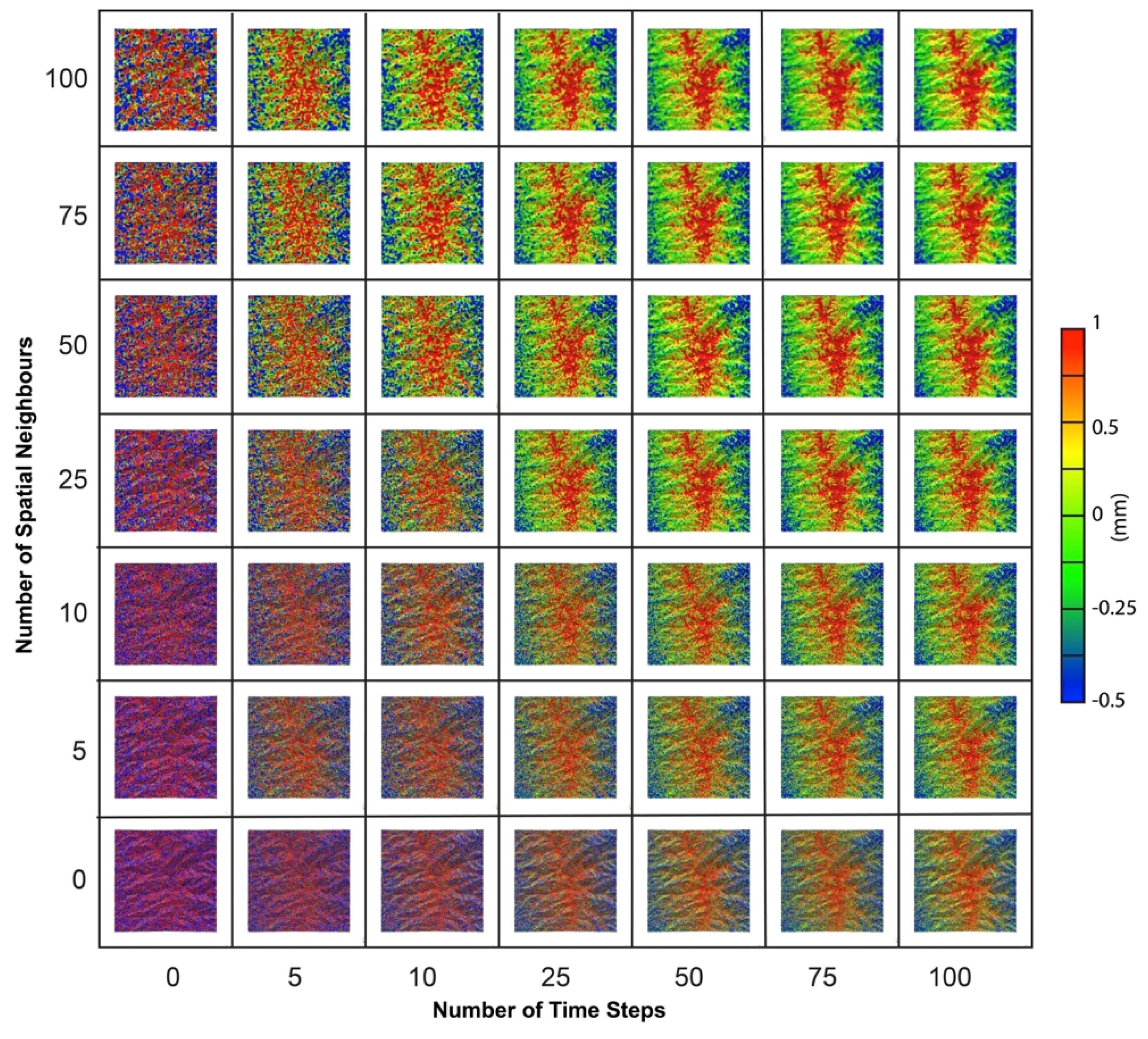
For a practical combination of space and time neighbours, filtered results for various spatial neighbours and time steps between 0 and 100 were compared (
Figure 7) at a constant resolution. Every combination results in different advantages and disadvantages. Filtered results with a low number of time steps, and spatial neighbours result in an inability to resolve the true signal. A high degree of spatial neighbours and a low number of time steps result in a degree of smoothing and difficulty in resolving the signal. Conversely, a high number of time steps and a low number of spatial neighbours results in high spatial resolution of the signal, but also a high degree of noise. Ideal results are obtained from combinations of neighbours in the upper right quadrant of
Figure 7; combinations where neither space neighbours nor time steps are dominant.
Figure 7.
Filtered synthetic DEM distances for a signal-to-noise ratio of 0.33 for combinations of space and time neighbours.
Figure 7.
Filtered synthetic DEM distances for a signal-to-noise ratio of 0.33 for combinations of space and time neighbours.
3.2.3. Noisy Reference and Calibration
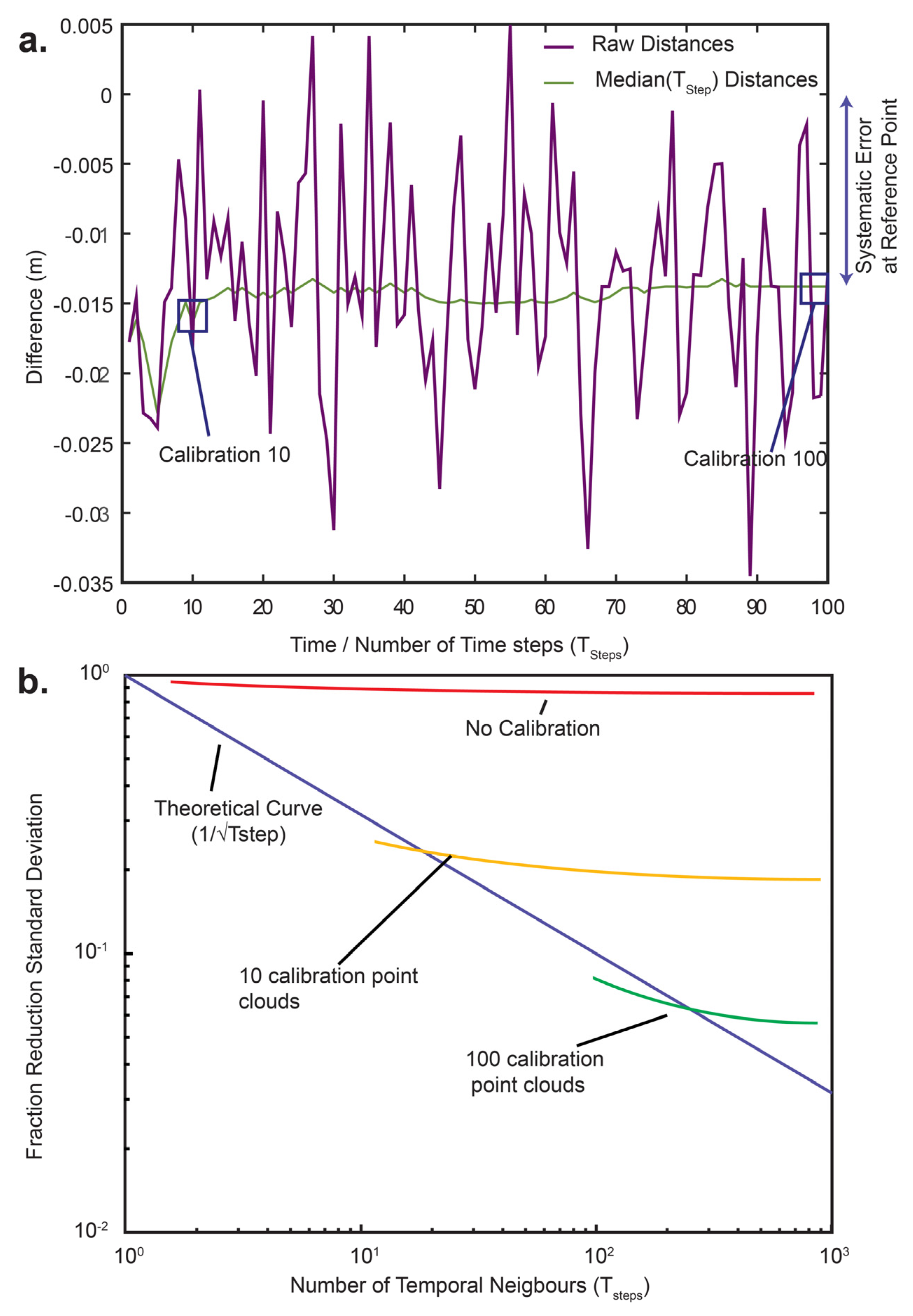
If a noisy reference point cloud is used for distance calculations, there will be an additional systematic error inherent in the reference value. The noise is random in space, but systematic in time, because a constant reference is used. To test the effect of calibration, one thousand digital elevation models with a Gaussian noise (σ = 0.015 m) and no induced displacement were constructed. The first point cloud of the thousand was the reference point cloud, and between 0 and 100 calibration point clouds were tested. For each point in the reference point cloud, median distances were calculated for each of the calibration point clouds. For each point, the median distances as a function of time step were calculated (
Figure 8a). After 10 time steps, the median curve began to converge on the systematic error for each point. With increasing time steps, the median value became closer to the systemic error of that point.
The fraction reduction in the standard deviation of the point cloud distances was calculated as a function of time steps for no calibration, for 10 calibration point clouds and for 100 calibration point clouds, alongside the theoretical reduction (1/√n) (
Figure 8b). There is minimal reduction in the standard deviation without calibration. This is because the systematic error at each point in the reference contributes to this standard error. Using 10 and 100 point clouds for calibration resulted in the theoretical standard error reduction when the time steps for filtering were close to the respective number of calibration point clouds used. In both cases, using larger filtering time steps than the number of point clouds used for calibration did not significantly reduce the standard error. It can therefore be concluded that an ideal number of calibration point clouds is equal to the planned number of filtering time steps.
Figure 8.
(a) Raw distances for a single point in the reference point cloud as a function of time and median filtered values as a function of time step for the calibration point clouds. (b) Standard error reduction for: no calibration, for 10 calibration point clouds and for 100 calibration point clouds compared to the theoretical reduction.
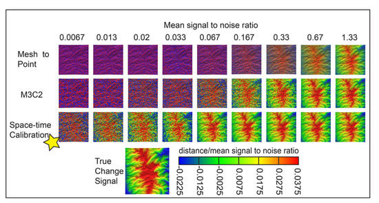
3.2.4. Comparison with Existing Methods
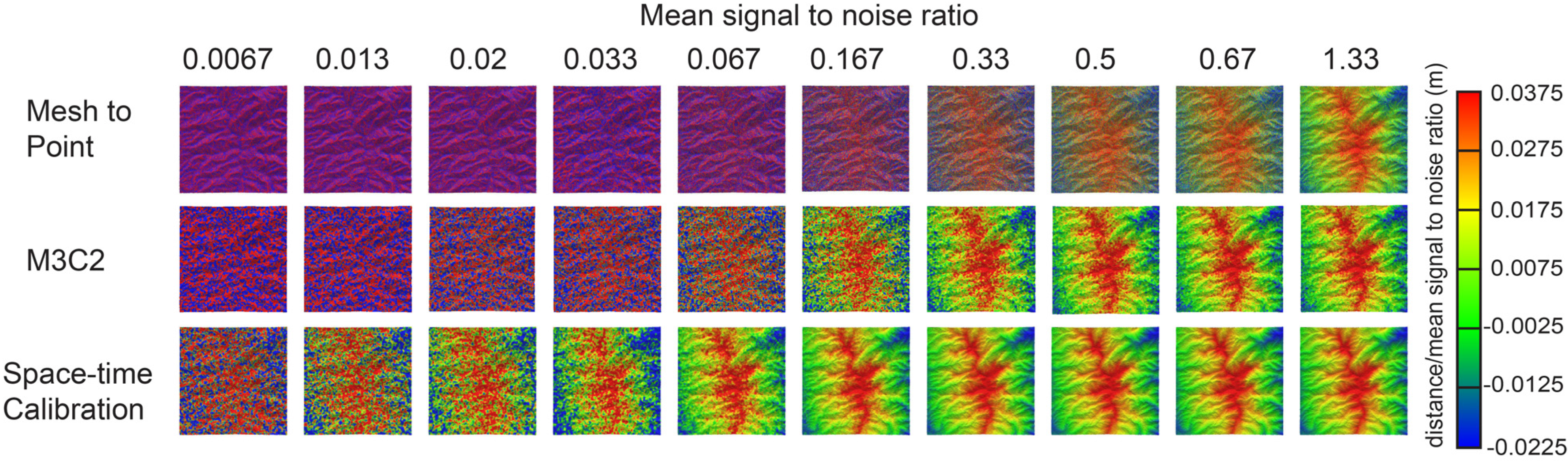
The combined space time calibration filtering technique was compared to the application of the mesh to point distance algorithm and with the M3C2 algorithm [
15] using a noisy reference. The comparisons were made by applying each algorithm to the synthetic case with a mean signal-to-noise ratio varying from 0.00067 to 1.33 (
Figure 9). For consistency, the normal scale for the M3C2 algorithm and space time calibration were set to a 1-m diameter, and the projection scale and spatial neighbourhood for averaging were kept the same at a 0.4-m diameter (50 points). For the space time calibration case, 50 calibration point clouds and a time step of 50 were used. The M3C2 algorithm uses position averaging, whereas space-time calibration uses averaging of point cloud distances.
The space time calibration algorithm performed the best as compared to the mesh to point algorithm and the M3C2 algorithm. A signal between 1.3% and 3.3% of the standard deviation of noise was detected using this approach, an order magnitude better than M3C2 and close to two orders of magnitude better than the mesh to point algorithm. Note that the space-time calibration algorithms uses a similar distance calculation methods as M3C2, with minimal position averaging. The performance of the algorithm comes from averaging on point cloud distances.
Figure 9.
Comparison of the M3C2 algorithm, mesh to point algorithm and the space-time calibration algorithm in detecting a signal over various signal-to-noise ratios.
Figure 9.
Comparison of the M3C2 algorithm, mesh to point algorithm and the space-time calibration algorithm in detecting a signal over various signal-to-noise ratios.
4. Results: Application of the Algorithm
4.1. Application of the Algorithm: Indoor Experiment
A controlled experiment was conducted in a laboratory to test the capability of the algorithm to detect very small displacements (at the sub-mm to mm scale) with real TLS data. An Optech Ilris 3D LiDAR scanner was used for this experiment, which has a manufacture-specified range accuracy of 7 mm and an angular accuracy of 8 mm at a 100-m distance [
43]. The scanner was set up 4.6 m from the target, in an indoor setting. The target consisted of a solid wood board with various irregular shapes fastened to it; the same target as in [
20].
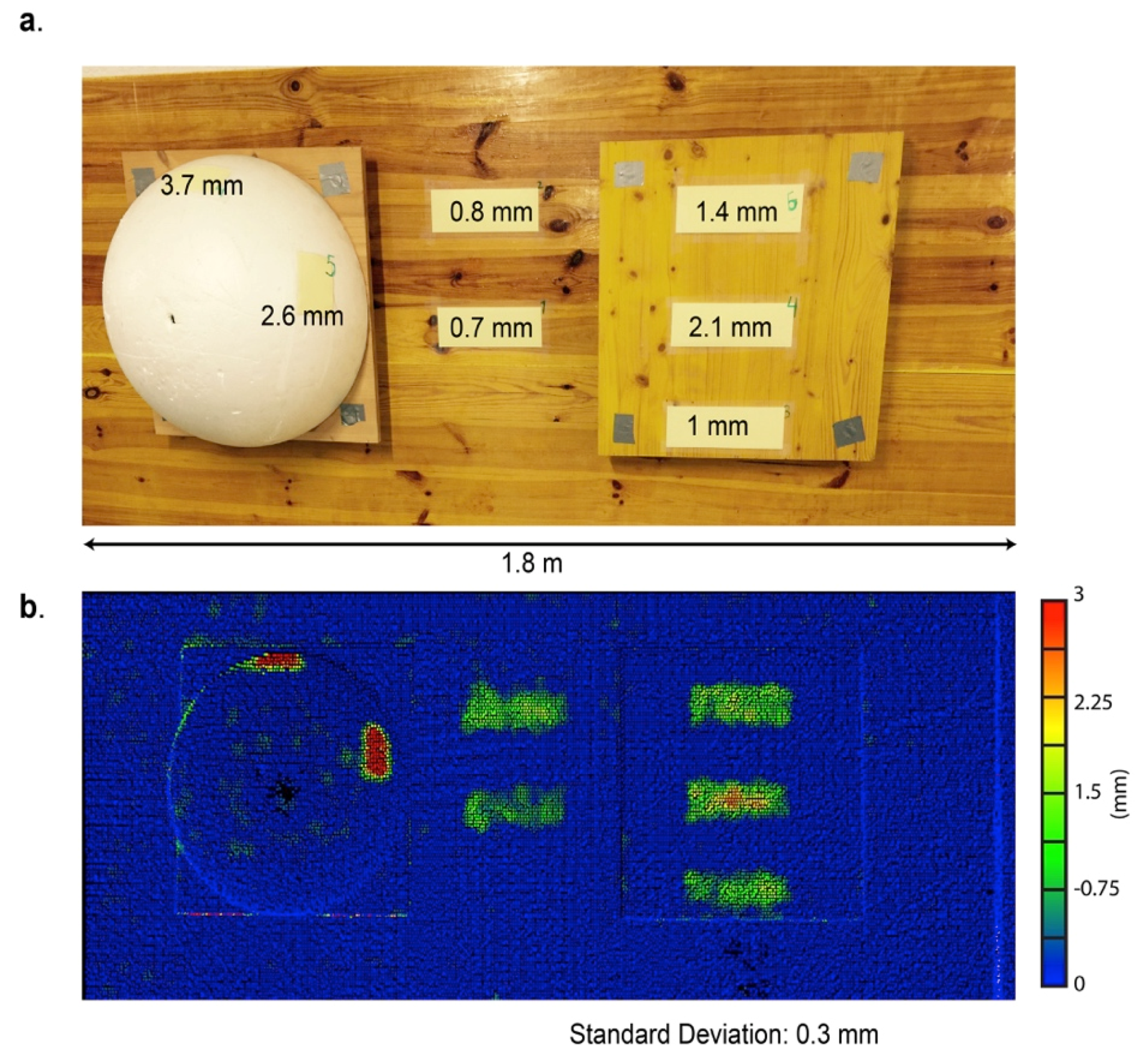
The target was first scanned a total of 50 times at a mean point spacing of 6 mm. These first 50 scans, with no induced displacements, comprise the calibration point clouds. Following the calibration scans, test pieces of cardboard (200 mm wide and 70 mm in height) were adhered at seven different locations on the target (
Figure 10a). A stack of 20 cardboard pieces was measured using calipers, indicating that each single piece is 0.2 mm in thickness. At each of the five flat surface locations, individual pieces of cardboard ranging between one and five pieces were combined to increase the size of the objects, thereby simulating displacement (
Figure 10a). To test the ability of the algorithm to detect displacements in oblique directions to the scanner, induced changes of four and five pieces of cardboard (100 mm wide and 70 mm in height) were added at two locations on a half sphere at an approximate angle of 45° to the laser incidence ray (
Figure 10a). Following the addition of induced displacements, the target was scanned an additional 50 times at the same scanner location to generate the data point clouds.
Scanning the same target continuously rarely results in the same physical pattern of scanned points; this is the result of random point spacing. For point cloud comparison, a best-fit alignment routine is applied to ensure good agreement between successive point clouds. An application of the iterative closest point (ICP) algorithm in Polyworks [
41] was used to align each data point cloud to a single reference scan. There is a systematic component of alignment error introduced when performing the ICP, but this is systematic only for single comparisons. With multiple comparisons, this error is random in time and is reduced using the temporal component of the filtering algorithm.
The induced displacements were measured by comparing the mean difference of each induced area between a combined 50 reference/calibration point clouds and a combined 50 data point clouds. Measured thicknesses are outlined in
Figure 8a.
The first step of the filtering approach, calculation of the reference point cloud normals and the distance to the calibration set, was carried out using a 0.1-m normal scale radius and a projection scale of 0.008 m. The systematic error (calibration value) for each point was calculated with all 50 calibration point clouds with no induced change. The standard deviation in this case represents the systematic error in the reference scan and is subtracted from the filtered data point clouds in the next step. The precision of the calibration standard deviation in this case allows filtering down to 1/100th mm.
Following the calculation of the calibration value, distances from reference to point clouds with induced change were calculated (
Figure 10b). A time step equal to the total number of scans (50) was applied with 15 spatial neighbours. Post filtering and calibration, the standard deviation was calculated to be 0.3 mm, corresponding to an LoD of 0.6 mm.
Figure 10.
(a) Experimental setup: seven stacks of cardboard of various thicknesses were adhered to a wood board and a Styrofoam half cylinder. (b) Filtered change detection results using 50 calibration scans, a time step of 50 and 15 spatial neighbours.
Figure 10.
(a) Experimental setup: seven stacks of cardboard of various thicknesses were adhered to a wood board and a Styrofoam half cylinder. (b) Filtered change detection results using 50 calibration scans, a time step of 50 and 15 spatial neighbours.
All seven areas of induced displacement were detected, and noise was reduced throughout the scene. Distances at the center point of the five areas of induced change normal to the scanner ray ranged between 0.7 mm and 2.1 mm, and distances on the half sphere were 2.6 and 3.7 mm, respectively. The measured induced displacements are generally higher than the summed thickness of the stacked cardboard at each location. This is likely due to air between the sheets of paper and between the sheet and the wood test board and/or as a result of difficulty in measuring the induced changes of this magnitude accurately with conventional measuring techniques.
4.2. Application of the Algorithm: Deformation Case Study
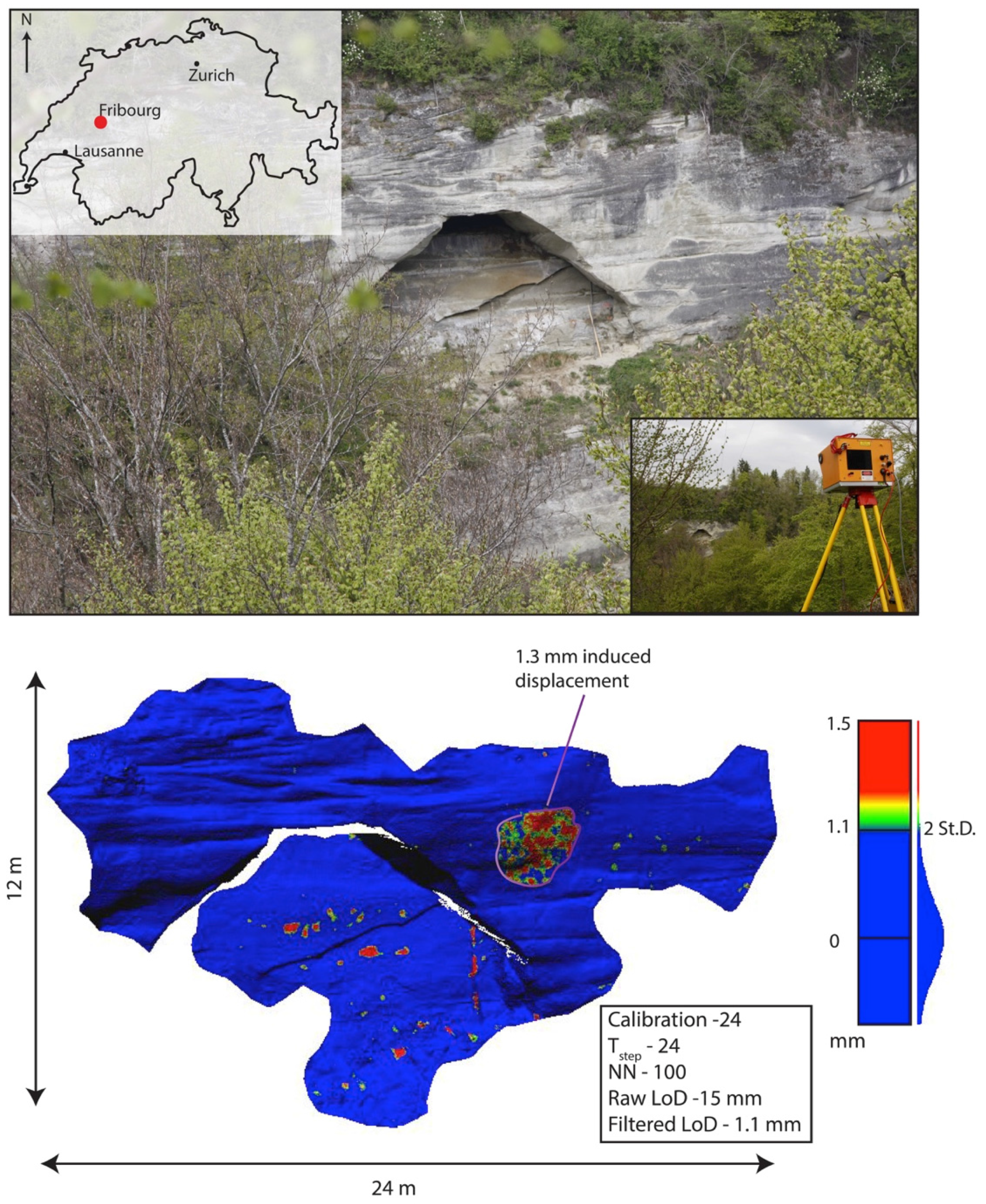
The algorithm was tested in real field conditions to determine practical survey LoDs for a cliff located in Le Gotteron River valley, outside the city of Fribourg in the Canton of Fribourg, Switzerland (
Figure 11). The site consists of an exposed section of bedrock on the side of the river valley composed of a sequence of siltstone and sandstone with a planar slab of bedrock bounded by a near vertical open daylighting joint.
Figure 11.
(Top) Survey setup at Le Gotteron valley near Fribourg, Switzerland. (Bottom) Filtered displacement using 24 calibration point clouds, a Tstep of 24 and 100 spatial neighbours. This resulted in an LoD of 1.1 mm and the detection of a 1.33-mm area of synthetic displacement.
Figure 11.
(Top) Survey setup at Le Gotteron valley near Fribourg, Switzerland. (Bottom) Filtered displacement using 24 calibration point clouds, a Tstep of 24 and 100 spatial neighbours. This resulted in an LoD of 1.1 mm and the detection of a 1.33-mm area of synthetic displacement.
An Optech Ilris 3D-LR long-range scanner was used with Enhanced Range (ER) mode. This scanner has a manufacturer-specified range at 80% reflectivity of 3000 m (~1500 m for rock slope studies), a scan frequency of 10,000 Hz, a range accuracy of 7 mm at 100 m in ER mode and 8-mm angular accuracy [
23]. The slope was scanned a total of 54 times at five-minute intervals with a mean distance of 200 m. Each scan consisted of approximately 360,000 points with a mean point spacing of 25 mm.
Raw point clouds were processed using the IMAlign module of Polyworks [
41]. This consisted of manual removal of vegetation and outlier points and application of the ICP routine to align all point clouds to the reference point cloud. The alignment residual at one standard deviation ranged from 7 to 8 mm. Distances between the reference point clouds, and each of the remaining 53 data/calibration point clouds was calculated using a normal scale of 10 m and projection scale of two times the mean point spacing (50 mm).
The first 24 point clouds after the reference point cloud were used for calibration. A synthetic displacement of 1.3 mm normal to the slope face was introduced in the upper right quadrant of the outcrop in the remaining data point clouds, since no real deformation was anticipated during this short survey period. A time step of 24 and a spatial neighbourhood of 100 were used to filter the calculated differences. This resulted in a standard deviation of 0.55 mm, making the per point level of detection for the slope at 95% confidence (1.96 standard deviations) at 1.1 mm.
An area consistent with the induced displacement was detected in the upper right quadrant of the slope (
Figure 11). Small areas of displacement in the 1- to 3-mm range were detected in the lower portion of the outcrop. It is not clear whether these are outliers or real displacement. The displacement could be the result of thermal expansion and contraction [
44].
4.3. Application of the Algorithm: Sediment Flux
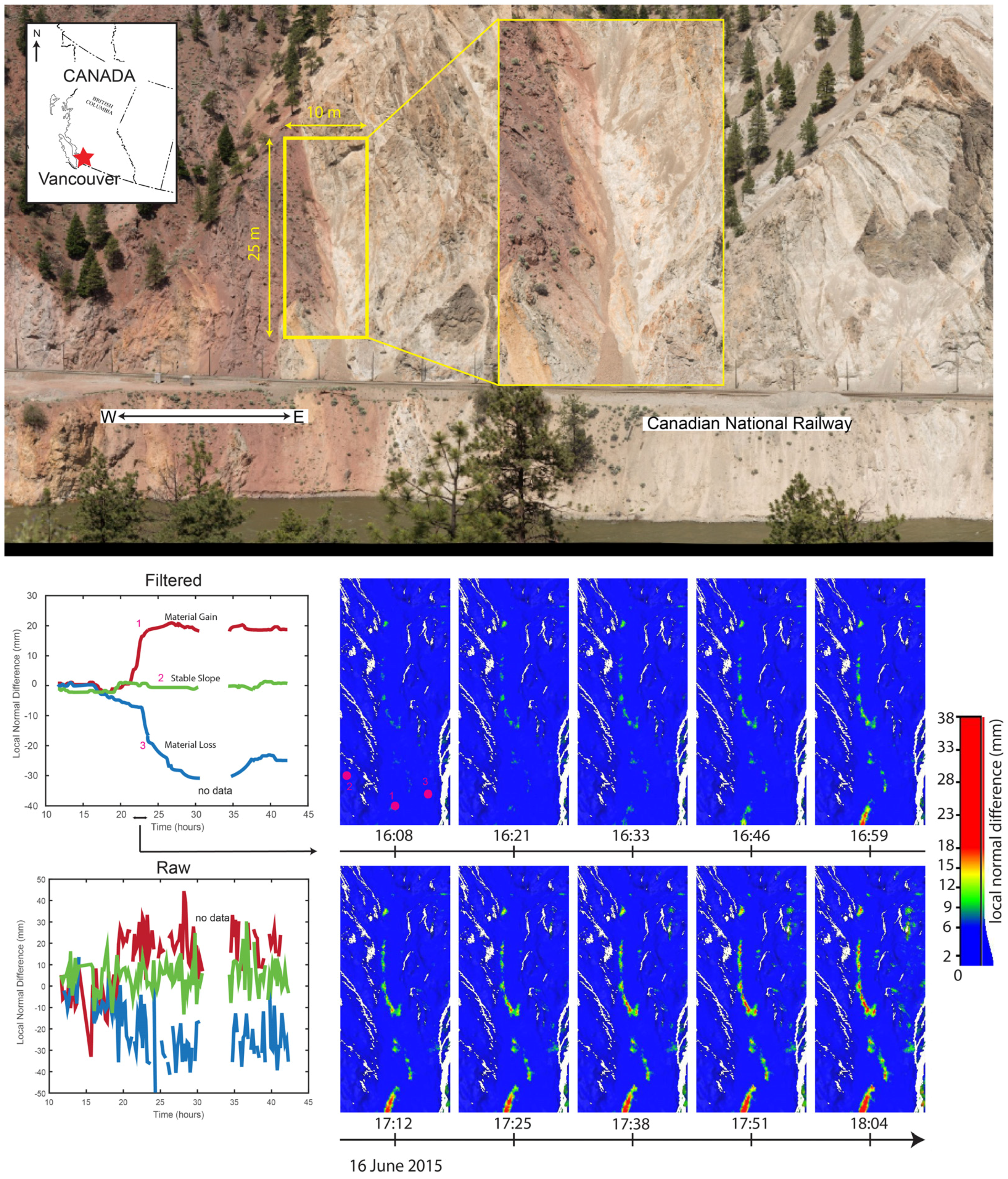
The algorithm was applied to the study of small-scale sediment flux in a talus slope at White Canyon along the Canadian National (CN) railway line in western Canada. The study site consists of a section of a complex morphology rock slope consisting of a weathered amphibolite quartzo-feldspathic gneiss in the eastern section and a weathered red conglomerate to the west. Sediment flux in a gully located along the contact between these two units were studied in detail (
Figure 12).
An Optech Ilris 3D-ER (enhanced range) laser scanner was used to scan the section of the slope continuously between 15 and 17 June 2015, for a total of 40 hours. Each scan took approximately 12 minutes to collect 1.8 million points of a larger area consisting of the gully and surrounding slope. Each point cloud was collected at a mean point spacing of 80 mm at a mean distance of 380 m. During the period of this study, a forest fire less than 10 km away resulted in less than ideal atmospheric conditions.
The point clouds were registered in the IMinspect module of Polyworks using an application of the ICP algorithm with a custom macro, which automatically aligned all point clouds to the reference point cloud with no manual interaction. The first 25 point clouds following the reference point cloud were used for calibration. A time step of 25 was used with 25 spatial neighbours for averaging. The per point limit of detection at 95% confidence at 300 m, following application of the algorithm, was 2.2 mm. The whole slope LoD, including regions of low point density, low incidence and that are further from the scanner, was 6 mm. Note that the limit of detection needs to be assessed for each characteristic slope region, based on a statistical analysis of stable region distances.
Sediment flux was detected in several regions of the study area and was analyzed for the gully at the contact between the two geological units. One particular flux event was observed on the second day of scanning over a time period of 116 minutes (
Figure 12), from 16:08 until 18:04 on 16 June 2015. The accumulation zone was in the order of 6 to 18 mm in thickness and appears to progress continuously over the time period. This accumulation zones gives an indication of the path of travel and progressive nature of the talus movement.
Figure 12.
Application of the algorithm to a sediment flux study at White Canyon in western Canada (top inset). Lower left: raw and filtered displacement time series for three points, one with the accumulation of material, one with the loss of material and one of the stable slope and the same time series. Lower right: change detection map for the accumulation area of the gully for a 116-minute period where sediment flux was observed.
In this particular case, the magnitude of displacement occurring over the specified time step is larger than the limit of detection achieved, and a shorter scan time or shorter time step is warranted. This likely resulted in a prolongation of the event by the convolution of the temporal filter with the noisy displacement signal. This can occur if the limit of detection achieved by applying the filtering algorithm is within the same order of magnitude as the real change occurring over the time step. To avoid this, a time step should be chosen so that the expected real change occurring during the time step is less than the limit of detection achieved by applying the filter.
5. Discussion
The proposed approach is ideal for applications where a small level of detection is necessary or desirable. In practice, with a well-designed data collection program and in ideal conditions, the application of this approach can lead to an order of magnitude or greater improvement in the single point level of detection. For complex slope environments, where target distance and point densities are variable, an assessment of error is necessary by analyzing the residual differences of a representative stable area. For most applications of this algorithm, a level of detection similar to that of radar systems can be achieved. Unlike techniques employing smoothing or averaging of the point positions (or point coordinates), this approach is applied to point cloud differences only, which is consistent with [
20]. Calculation of the median value on a large enough sub-group of point differences results in robust estimation of the parametric mean, even if outliers are present in the population.
The approach is adaptable and can be customized to specific survey site requirements. Alternative distance calculation methods can be substituted, such as point-to-point, one-dimensional point-to-mesh, M3C2,
etc. The improvement in level of detection is attained by averaging neighbours in either space or time domains; thus, a desired reduction can be obtained from a number of different neighbour combinations. This allows the algorithm to be adapted to detect signals with a range of rates of change and spatial extent without smoothing the signal. Compared to earlier approaches using space filtering only [
20] or other approaches using position averaging [
15], the addition of time steps results in a higher spatial change resolution and the ability to detect smaller features. The number of time steps must, however, take into account the expected rate of change. Furthermore, the point cloud acquisition rate must also be taken into account; this must be much faster than the rate of signal change and is limited by the acquisition rate of the scanner in use. This is because application of the time filter is equivalent to the convolution of the filter function with the noisy change function, which could cause the appearance of a reduced rate of change compared to reality. A time step should be used so that the change over the time step is less than the limit of detection achieved using that time step. This effect can be avoided either by reducing the time step or acquiring data faster. For example, a daily acquisition rate is suitable for an expected rate of change in the order of a few mm a year. In cases where very small spatial signal extents are expected, such as the development of small rock slope failures, a higher acquisition rate may be warranted to ensure sufficient reduction in the standard deviation of the mean and to reduce spatial smoothing.
This approach reduces random noise and systematic errors. Systematic errors result from using a common noisy reference point cloud to calculate distances or from alignment error or poor incidence angle. The use of calibration point clouds allows the calculation and removal of the systematic error specific to the reference point cloud. Convergence on the systematic error usually occurs around Time Step 10. Further use of calibration point clouds slightly increases the precision of the calibration values. For this reason, a calibration point cloud number close to that of the time step used will result in the theoretical reduction in the standard deviation. The use of calibration sets can also be a useful approach for any survey design, even if scanning is not conducted on a high temporal basis. For example, the first acquisition would consist of the reference scan and a frequent collection of point clouds to be used for calibration followed by data point clouds acquired at a lower frequency. Alternative techniques to removing the systematic error caused by using a noisy reference include using alternative de-noising techniques on the reference, perhaps fitting a surface model to a densely acquired reference point cloud, or marching forward the reference point cloud through time. The latter proves to be inefficient due to an increase in computational time by a factorial factor.
Compared to other point cloud comparison approaches, such as point to mesh, the M3C2 algorithm [
15] and 2D spatial filtering [
20], this approach provides a significantly better ability to detect small-scale change in 3D. Application of the algorithm without the temporal filtering and with the calibration component provides an improved spatial resolution compared to the M3C2 algorithm with similar input parameters and has the benefit of reducing systematic errors. M3C2 relies on position averaging in both the reference and data point clouds for noise reduction, which in high roughness or curvature terrain noise and can cause artifacts if too large a projection scale is used. Note that the proposed algorithm uses a modified M3C2 distance with a minimum projection scale and then applies averaging to the point cloud differences. The addition of the temporal filter with calibration provides an order of magnitude improvement in the ability to detect change. This can be advantageous for the study of precursor deformation of small magnitude landslides, the study of small-scale sediment transport and erosion and even small-scale deformation in civil engineering works. The application of the algorithm does require the effort of continuous scanning and the storage and processing of a large amount of 3D data.
Table 1 provides a summary of the advantages and disadvantages of other point cloud comparison methods and their best application.
Table 1.
Comparison of several point cloud distance calculation algorithms for small-scale change detection.
Table 1.
Comparison of several point cloud distance calculation algorithms for small-scale change detection.
| Method | Advantages | Disadvantages | Best Application |
|---|
| Mesh to point or mesh to mesh change detection | Shortest distance calculation allows interpretation of change in different directions; some reduction in noise through creation of a mesh. | Artefacts caused by the creation of an average mesh surface. | Not recommended for small-scale change detection. |
| M3C2 | Change in three dimensions along the local point cloud normal; some reduction noises through position averaging. | Increasing the projection scale leads to artefacts from position averaging; not as effective as difference averaging. | Recommended for change detection where a high temporal sampling cannot be achieved and in complex terrain. |
| Spatial filtering (with calibration) | Can be applied to differences from any change detection method; better reduction of noise compared to position averaging. | Decrease in spatial resolution for the detection of change when a large number of neighbours is used. | Recommended for change detection where a high temporal sampling cannot be achieved, in complex terrain and where the expected area of change is large compared to point spacing. |
| Space-time filter (with calibration) | Effectively reduces Type 1 and Type 2 errors and allows an increase of 1 to 2 orders of magnitude or greater in the per point limit of detection. | Can only be used in frequent/continuous scanning scenarios. | Recommended for studies where high temporal sampling can be achieved and for studying small-scale change detection. |
6. Conclusions
A 4D filtering and calibration approach that takes advantage of the point redundancy of TLS data in space and time was presented, compared to existing techniques and applied to several case studies. The method provides an improvement over 2D filtering techniques, which average point cloud differences along one dimension only, and techniques involving positioning averaging, such as point to mesh comparison or the M3C2 algorithm. The approach uses a modified M3C2 distance calculation algorithm that limits position averaging and is followed by the application of spatial and temporal averaging. Furthermore, this technique can reduce systematic errors through the calibration procedure. With appropriate selection of the input parameters, an order to two orders of magnitude in the level of detection can be achieved compared to existing point cloud comparison techniques. The proposed filtering approach is also adaptable to any point cloud distance method.
With continuous TLS scanning, similar limits of detection as radar systems can be achieved with the added benefit of obtaining 3D displacements and dense and accurate point clouds. This is demonstrated through several case studies. Significant improvement in the limit of detection for change was achieved in a rock fall hazard scenario and in a complex slope where small-scale talus flux was occurring. An improvement in the limit of detection will allow the detailed study of terrain changes at an unprecedented level of detail in 3D. This will be particularly beneficial for studying the precursor phase of landslides and other small-scale geomorphological processes.


 ,
, 


