Abstract
Monitoring unstable slopes with terrestrial laser scanning (TLS) has been proven effective. However, end users still struggle immensely with the efficient processing, analysis, and interpretation of the massive and complex TLS datasets. Two recent advances described in this paper now improve the ability to work with TLS data acquired on steep slopes. The first is the improved processing of TLS data to model complex topography and fill holes. This processing step results in a continuous topographic surface model that seamlessly characterizes the rock and soil surface. The second is an advance in the automated interpretation of the surface model in such a way that a magnitude and frequency relationship of rockfall events can be quantified, which can be used to assess maintenance strategies and forecast costs. The approach is applied to unstable highway slopes in the state of Alaska, U.S.A. to evaluate its effectiveness. Further, the influence of the selected model resolution and degree of hole filling on the derived slope metrics were analyzed. In general, model resolution plays a pivotal role in the ability to detect smaller rockfall events when developing magnitude-frequency relationships. The total volume estimates are also influenced by model resolution, but were comparatively less sensitive. In contrast, hole filling had a noticeable effect on magnitude-frequency relationships but to a lesser extent than modeling resolution. However, hole filling yielded a modest increase in overall volumetric quantity estimates. Optimal analysis results occur when appropriately balancing high modeling resolution with an appropriate level of hole filling.
Keywords:
point cloud; surface modeling; laser scanning; lidar; change detection; rockfalls; geohazards 1. Introduction
The management of slope hazards (e.g., rockfalls, landslides) along transportation corridors and in metropolitan settings poses a significant challenge to public officials. Slope hazards are not only costly, but they present a significant threat to life in many parts of the world [1]. Remote sensing technologies such as terrestrial laser scanning (TLS, also known as terrestrial lidar) show promise for the rapid assessment of unstable cliffs. Several studies have successfully utilized TLS for slope stability assessments and monitoring. Jaboyedoff et al. [2] and Abellán et al. [3] provide a detailed review of applications, benefits and challenges of lidar for landslide and rock slope stability studies. Kemeny and Turner [4] evaluated the use of laser scanning for highway rock slope stability analysis and found that TLS offered several advantages compared with traditional techniques, including safety, accuracy, access, and analysis speed.
Multi-temporal datasets acquired using TLS technology enable detailed change analyses through time [5,6,7,8,9,10,11,12,13,14,15,16,17,18,19,20]. These repeated surveys enable engineers and scientists to understand the progressive patterns of failures and discern the influence of environmental conditions [21,22,23,24,25,26,27], which lead to those failures. Comparisons of each TLS survey enable the quantification of erosion rates and surface deformation, which can be used to analyze the pattern and propagation of displacements that have taken place over the monitoring period. For example, Lato et al. [28] demonstrate how rockfall hazards along transportation corridors can be monitored using mobile laser scanning (MLS) on both railway- and roadway-based systems. In both situations, MLS provided increased efficiency, safety, and the ability to investigate hazards compared with TLS.
Researchers such as [17,26,29,30,31,32] have then used these multi-temporal datasets in order to establish magnitude–frequency relationships to show the frequency distribution of large to small volumes of material release. Such distributions provide important information needed to support landslide hazard and risk assessment [31,32]. Tonini and Abellan [33] present a novel approach for rockfall detection from repeat lidar surveys by generating clusters based on a K-nearest neighbors algorithm with clutter removal capabilities. The authors of [34] build on the process developed in [33] with a semi-automatic approach to calculate volumes of each rockfall cluster to generate magnitude–frequency relationships.
To perform meaningful volumetric change analyses to develop these magnitude-frequency relationships, point clouds are commonly triangulated to produce continuous surface models. However, surface modeling methods can be difficult to employ on surfaces exhibiting high amounts of topographic variability and morphologic complexity. Further, the point sampling on the cliff surface is not uniformly distributed. Many modeling techniques (e.g., [35,36,37,38,39]) have been developed for artificial objects, which are generally smooth and transitions are well defined. Such approaches often do not translate well to creating topographic models where surface changes can vary significantly across small distances [40]. This, in turn, leads to topological artifacts. For accurate volumetric change analysis, surfaces must be free of intersecting triangles, have consistent facet normal orientations, and be free of data gaps (i.e., holes) in the areas to be analyzed. Processing procedures to generate such topologically correct models often require significant manual editing, which can be difficult and cumbersome. Moreover, while a variety of hole filling approaches exist, they are often dependent on the modeler’s interpretation, and thus include an element of subjectivity. The influence of these techniques on the resulting volumetric analyses is often not considered or clearly documented.
Objectives
This paper builds on previous work to present a new, fully automated approach to perform change detection and identify individual rockfalls on complex rock slopes. Specifically, the paper introduces:
- A streamlined approach to analyze time series point clouds to isolate individual failure clusters (i.e., rockfall events) on the rock slope, to quantify volumes of each cluster, and to generate magnitude–frequency relationships from those clusters.
- An evaluation of the influence of surface modeling parameters such as the degree of hole filling and modeling resolution on the resulting magnitude–frequency relationships, rockfall detection, and overall erosion volume computations. In this study, resolution is defined in terms of the model resolution, rather than actual sampling resolution.
While an interesting, semi-automated approach for rockfall clustering [33,34] has recently been developed, the proposed approach is an alternative method of performing this analysis that is fully automated. Additionally, [33,34] do not consider the influence of hole filling and modeling resolution on the resulting magnitude-frequency relationships, but rather work directly on the point cloud.
The proposed approach was applied to several study sites with active, unstable rock slopes in the State of Alaska, U.S.A. Results from three representative study sites are presented to demonstrate the effectiveness of this approach. However, it is worth noting that the level of automation developed by this study has enabled this procedure to efficiently evaluate rockfalls along much larger sections of highway than what can be presented in this paper.
2. Methodology
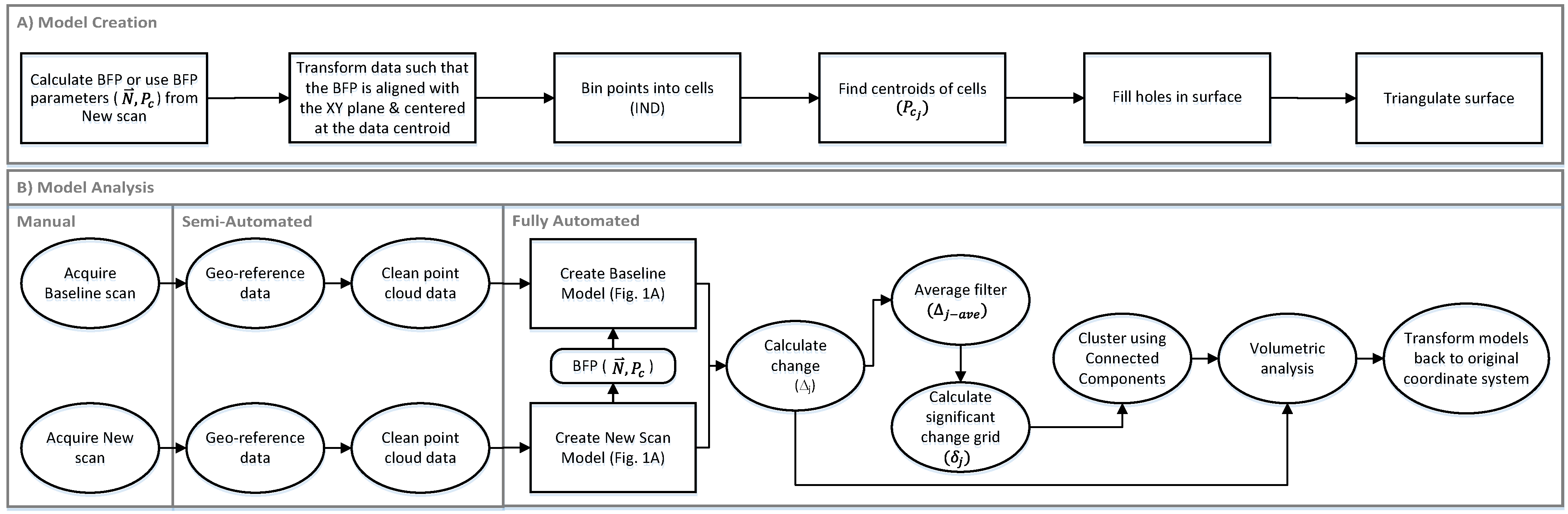
Figure 1 presents an overview of the methodology, and details for each step will be discussed briefly in this section. Figure 1A describes the process for model creation, and Figure 1B provides the steps for the model analysis. For change analysis, the baseline surface model is created from a point cloud from a previous survey. However, this model is created simultaneously with the new model (following the same process) such that they are both generated in the same reference plane. When a corridor is highly sinuous, it must be tiled into smaller segments to apply this approach for optimal results since the data will no longer be reasonably projected to a plane. However, such tiling is common in most lidar processing over long distances.
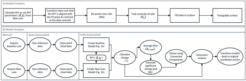
Figure 1.
Flowchart of key steps of the methodology (BFP = Best Fit Plane). (A) Model creation; (B) Model analysis.
Figure 1.
Flowchart of key steps of the methodology (BFP = Best Fit Plane). (A) Model creation; (B) Model analysis.
2.1. Data Acquisition
Figure 2 shows the location of the study sites within Alaska, U.S.A. Three surveys were completed at each site during the summers of 2012, 2013, and 2014. A summary of equipment used, estimated accuracies and typical point sampling intervals is provided in Table 1. This section will describe the details of each survey because the scope and equipment used varied between surveys.

Figure 2.
Topographic relief map showing the location of Study Sites A, B and C in Alaska, U.S.A. (Shaded relief map courtesy of the Earth Systems Research Institute, ESRI).
Figure 2.
Topographic relief map showing the location of Study Sites A, B and C in Alaska, U.S.A. (Shaded relief map courtesy of the Earth Systems Research Institute, ESRI).
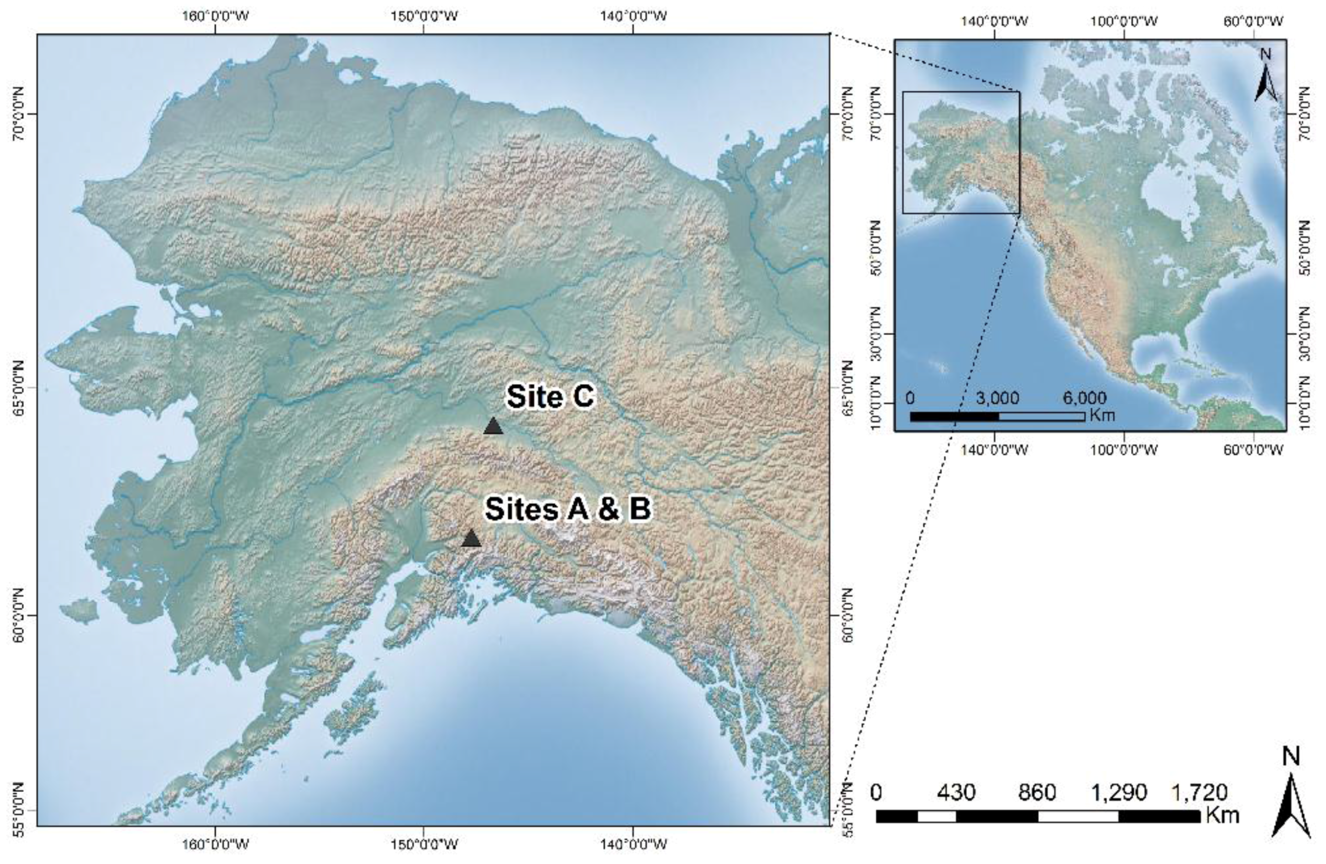

Table 1.
Summary of survey data collected including typical accuracies and point sampling intervals on the cliff surface.
| Survey Date | Equipment Used | Site A | Site B | Site C | |||
|---|---|---|---|---|---|---|---|
| Accuracy (3D-RMS, m) | Typical Point Sampling (3D, m) | Accuracy (3D-RMS, m) | Typical Point Sampling (3D, m) | Accuracy (3D-RMS, m) | Typical Point Sampling (3D, m) | ||
| September, 2012 | Terrapoint Titan mobile laser scan system, Leica ScanStation 2, Leica GNSS1200 receivers, Leica 1201 total station | 0.10 | 0.05 | 0.10 | 0.05 | 0.09 | 0.08 |
| August, 2013 | Riegl VZ-400 TLS, Nikon D700 camera, and Trimble R8 GNSS receiver | 0.04 | 0.01 | 0.04 | 0.01 | 0.04 | 0.04 |
| July, 2014 | Riegl VZ-400 TLS, Nikon D700 camera, and Trimble R8 GNSS Receiver | 0.04 | 0.01 | 0.04 | 0.01 | 0.04 | 0.04 |
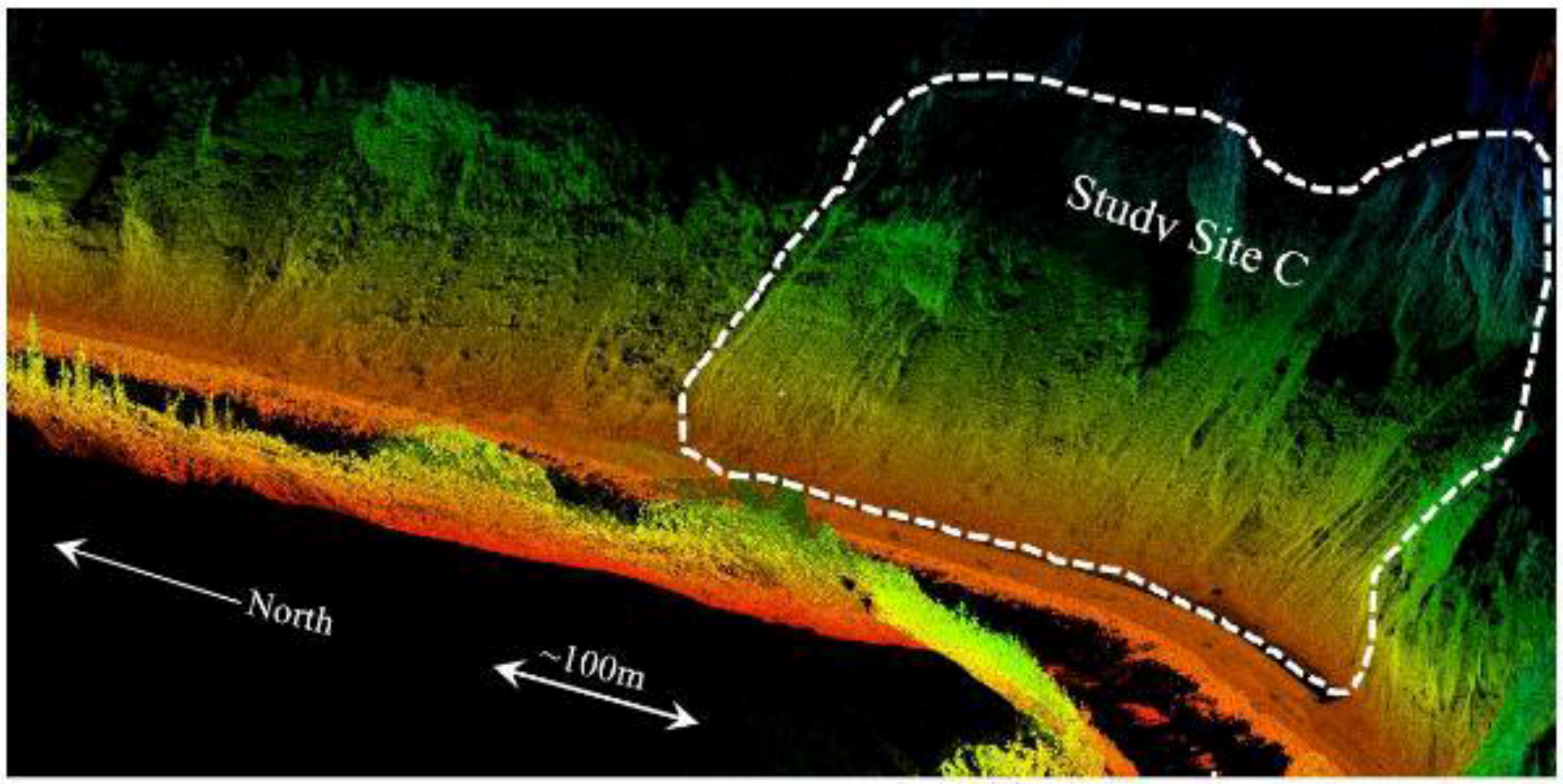
The 2012 survey (Figure 3) was completed using a mobile laser scan system with a few supplemental TLS setups in locations with tall cliffs. The mobile scan surveys were completed for two major roadways in Alaska: a 16 km segment of Glenn Highway (State Route 1) and a second 16 km segment of Parks Highway (State Route 3). Multiple passes were completed to increase point density as well as verify the accuracy and consistency of each pass since the canyon limits the line of sight to GPS satellites.

Figure 3.
Perspective view of a sample point cloud for a 1 km section of the Parks Highway obtained with combined TLS and MLS data. The dashed line highlights Study Site C.
Figure 3.
Perspective view of a sample point cloud for a 1 km section of the Parks Highway obtained with combined TLS and MLS data. The dashed line highlights Study Site C.
The 2013 and 2014 scan surveys were completed for relatively shorter segments each encompassing approximately 15 km in total for both Parks and Glenn Highway. These scans were obtained using a stop-and-go scanning approach utilizing field procedures very similar to those presented in [27] where the scanner is mounted on a wagon rather than a tripod for efficient data collection. Inclination sensors are also included in the scanner to correct for the scanner being out of plumb when conducted from the wagon platform. A digital SLR camera and a survey grade GPS receiver were mounted above the scanner with calibrated transformation offsets (translations and rotations) to the scanner origin. Atmospheric conditions (temperature, pressure, and relative humidity) were recorded and input into the laser scanner during data acquisition to correct distance measurements.
During the 2013 and 2014 data acquisition, scan positions were typically spaced at 50–80 m apart along the highway and covered a 360 degree horizontal field of view and a 100 degree vertical view (−30 degrees to +70 degrees from the horizontal plane).The resolution of the scans varied between 0.02 and 0.05 degree sampling increments. Each position was occupied for at least 20 min to enable sufficient time for Rapid Static GPS data logging. Six photographs encompassing a 360° view were acquired at each scan position.
2.2. Processing
Geo-referencing is a critical step to relate data from different dates, particularly in areas with active tectonic movement. Because each scan is normally recorded in its own coordinate system, one scan survey is not relatable to another unless it is transformed into a common coordinate system (Alaska State Plane Coordinate System Zone 4, North American Datum 1983 (2011) Epoch 2010.00, Geoid 12A). This process is generally accomplished through a least squares, rigid-body coordinate transformation, determining both rotations and translations along orthogonal axes, which results in the minimization of the sum of the square errors between point pairs (either from pre-marked targets or matching points in the point cloud).
For the static scans collected in the 2012 survey, reflective targets were placed throughout the scan scene, which were linked with a total station to ground control points established with RTK GPS. The coordinates of the base station were established using the static processing through the National Geodetic Survey Online Positioning User Service, OPUS [41]. The mobile lidar data was processed using proprietary software with direct geo-referencing from the GPS, Inertial Navigation System (INS), and scanner sensors on the mobile lidar unit.
For the 2013 and 2014 surveys, both the baseline and in-situ scans were geo-referenced following the methodology presented in [27,42] using the program PointReg. The methodology was developed for efficient surveying in dynamic environments (e.g., coastal areas, active landslides) where survey control can be difficult to establish and maintain. Although other geo-referencing procedures can be implemented, such as the approach implemented in the 2012 survey, the PointReg approach can minimize field time, since targets are not required [43].
During the field data collection, the operator obtains most of the geo-referencing transformation parameters needed for scan alignment. Translation vectors (X, Y, Z) were obtained for the scanner origin using the co-acquired GPS data (20 min for each scan), which were processed in OPUS-RS. These coordinates were corrected both for offsets between the scanner origin and GPS antenna reference point and accounting for a slightly out of level setup, typically < 2°–3°.
The leveling information (rotations about the X (roll) and Y (pitch) axes) is determined using internal inclination sensors in the scanner, avoiding the need to level the scanner. Silvia and Olsen [44] highlight the importance of these sensors and their ability to provide quality data for scan geo-referencing. The azimuthal values for scan positions are initially estimated using a digital compass and then converted into a rotation about the Z-axis (yaw). This angle is then improved using the least squares solution presented in Olsen et al. [42], which calculates the optimal rotation of a scan about the Z-axis (centered at the scan origin) to best fit with nearby points in neighboring scans.
The methodology utilized does not require each epoch to be registered together since the each survey is independently georeferenced into the same coordinate system. [27,42] have shown that the methodology provides consistent results between multi-temporal surveys. In addition, the geo-referencing was validated by examining concrete structures, roadways, guardrails, and other objects present in the scene that were observed to be stable with time.
Following geo-referencing, point cloud data is typically filtered [13] to eliminate unwanted features (e.g., passing vehicles, vegetation, reflections from wet surfaces, moisture in the air). Filtering processes vary substantially in the degree of user interaction required and the type and quantity of noise present. These data were all removed manually using Leica Cyclone and Maptek I-Site software by creating polygon windows around unwanted objects. Vegetation noise on the cliff face were also removed to the extent possible. Areas of dense vegetation with minimal ground points were simply removed entirely from the dataset. However, areas with sparse vegetation were carefully edited in smaller cross sections so that ground points were preserved. This editing results in a cleaned point cloud (P) with n points in the form:
Note that each point also has a mapped RGB color and Intensity (return signal strength) value as well; however, given that the majority of the analysis is focused on the geometric coordinates for change detection, these parameters will only be periodically discussed in this paper when relevant.
2.3. Surface Generation
Once a cleaned point cloud has been obtained, the next step is to determine the optimal plane for the triangulation, which is obtained by solving an eigenvalue problem to determine the best fit plane through the dataset (e.g., [45]). The plane is defined by a normal vector (N = {Nx, Ny, Nz}) and the centroid coordinates of the original dataset (Pc). (Note that for computational efficiency, one can use a fraction of the points in the dataset to estimate the normal of the plane, if desired).
Next, the necessary transformation to align the best fit plane with the XY plane can be represented as rotation about a vector or a quaternion [46,47]. The orientation is established such that the Z′ axis is positive away from the rock slope so that erosion values will be negative. The vector ρ is first calculated by the cross product:
where τz = {0,0,1}, represents a normalized vector for the Z axis (i.e., normal of the XY plane). The angle of rotation (α) can be found with the cross product, which can be simplified with τz as:
The resulting rotation vector and angle can then be represented as a quaternion [46] producing a rotation matrix, R, such that the transformed point coordinates can be calculated by:
Next, the minimum and maximum values for all points (p′) are found. The number of columns and rows for the grid structure with a cell size dimension of σ are calculated as:
Each point (p′) is then subdivided into the square grid cells based on a spatial index IND:
where:
Then, the centroid coordinates for each cell (j) are calculated from all m points within the cell:
Once centroids have been found for all cells, a hole filling operation can be completed to create interpolated points in cells with insufficient data. The specifics of the hole filling approach will be described in more detail in the next section. Following hole filling, the triangulation is then formed using the rules established in Olsen et al. [40] (Figure 4). In this approach, the positions of the centroids of four adjacent cells are evaluated to determine the appropriate connections to avoid intersections of triangles. Although there are five potential scenarios, only two triangulation patterns are needed, which can quickly be determined with a point in triangle test. This method proves to be very efficient because the cell centroids are structured and simple to connect with these rules.
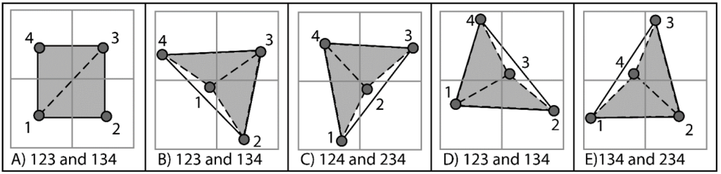
Figure 4.
Triangulation scheme adopted from Olsen et al. [40].
Figure 4.
Triangulation scheme adopted from Olsen et al. [40].

After triangulation, the centroids can then be transformed back to the original coordinate system:
Similar to averaging the X, Y, Z coordinates to determine the centroid coordinates, RGB color or Intensity values can be averaged for all points in the cell for texture mapping and further analysis.
2.4. Hole Filling
Data gaps (holes) are inevitable in any laser scan data because of obstructions that block the line of sight to the objects of interest. In particular, for this study, scanning needed to be completed relatively close (approximately 20–40 m) from the cliff face so that the equipment could be set up adjacent to the highway for accessibility. This close proximity to the cliff results in several portions of each scan being oblique to the surface, which results in more holes from topographic obstructions compared to scanning from vantage points with a better view further back from the cliff surface [27]. (It is noted that this problem can be somewhat mitigated by spacing scans closer; however, the increased number of setups reduces the amount of coverage possible in a given time window). Passing vehicles also resulted in several holes on the cliff surface in each scan.
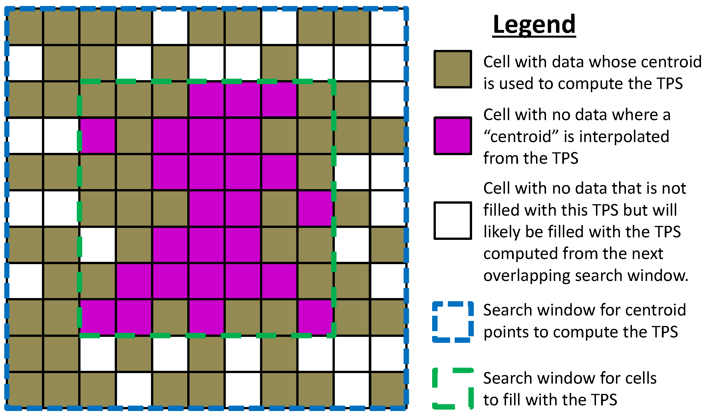
Holes in the model were filled by generating a thin plate spline (TPS) from the cell centroid points in cells surrounding the holes (Figure 5). Because the TPS technique is computationally inefficient across large point cloud datasets, a TPS is computed for a small window of the dataset at a time. However, note that large holes require a larger window size to be filled. To avoid poor fits in areas with sparse data, 50% of the cells in the window were required to have data in order for holes within that window to be filled. Also, to minimize artifacts and edge effects, holes are only filled in the center cells of the window. For purposes of this study, the window size is defined as the number of pixels included in each direction outward from the center pixel that are included for the hole filling. For example, with a window size of 5 (11 × 11 cells), all cells with data in the 11 × 11 cells were used to compute the TPS, but cells with holes were only filled in the center 6 × 6 cells (Figure 5). Note that the interpolated points are not used in the next overlapping window to compute the TPS.
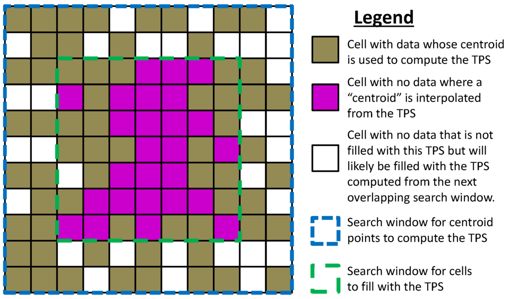
Figure 5.
Schematic illustrating the hole filling process using thin plate spline (TPS) interpolation.
Figure 5.
Schematic illustrating the hole filling process using thin plate spline (TPS) interpolation.
The computation of TPS was adopted from [48,49]. The TPS can be calculated from the centroid points for each cell within the search window through a linear equation system based on minimizing bending energy in the TPS. A regularization parameter (β ≥ 0) can control how tightly the TPS fits the input points. The solution of this linear equation system results in local influence weights (w) and coefficients (a) that can be used in the following interpolation equation to determine the z′ coordinate for the cells without data:
where x′ and y′ are the coordinates at the center of the cell without data in the transformed coordinate system. U is a weighting function based on the distance between the cell without data and each of the points in the subdatset that are used to compute the TPS.
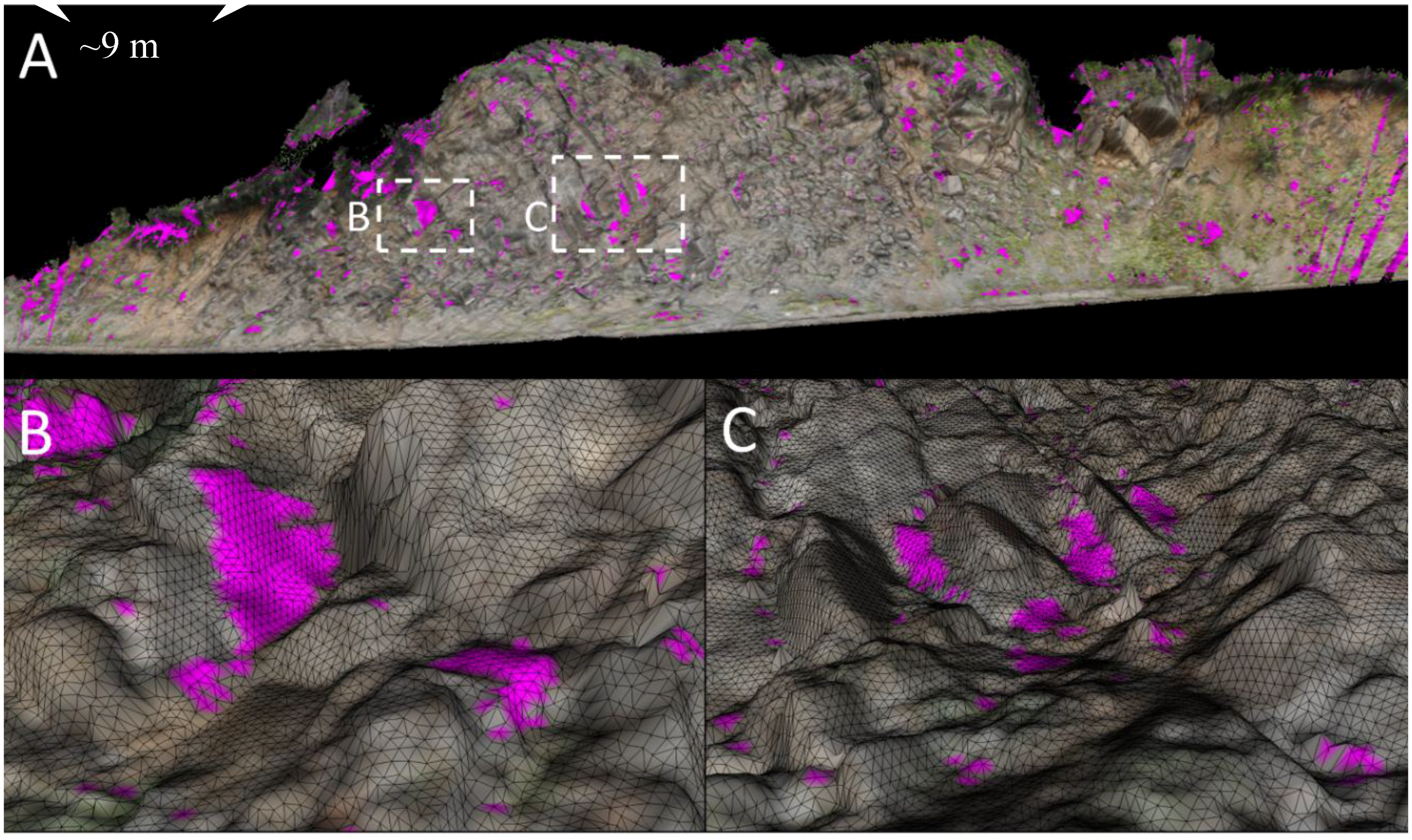
Figure 6 shows an example of hole filling in a surface model generated at Site A using the approach described above. In this example, both large and small holes can be filled across even larger data gaps by increasing the window size for visualization purposes; however, as with any technique, interpolation errors across these extents could generate significant problems for volumetric estimates, particularly on gradually eroding slopes. Hence, some judgment is necessary for implementation.
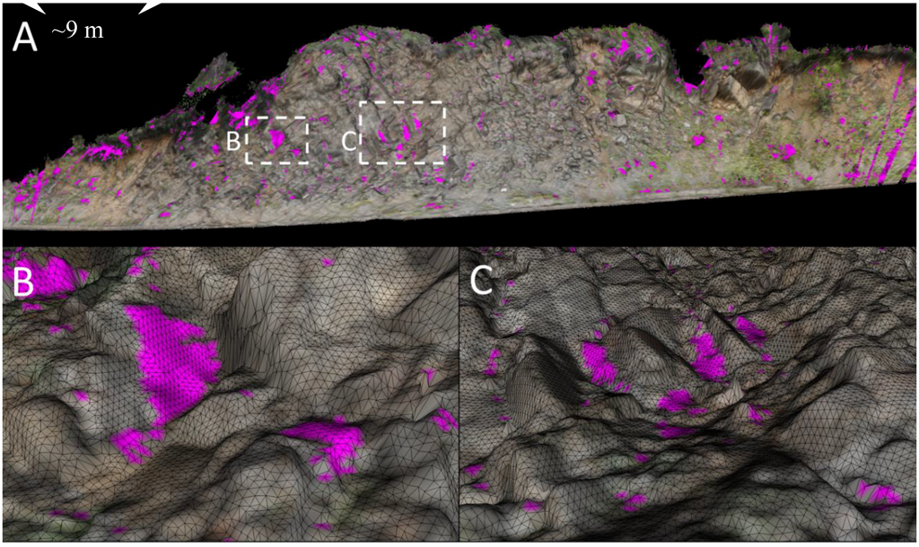
Figure 6.
Example of hole filling for the 2014 surface model for Site A using a grid cell size of 0.05 m and window size of 20 (i.e., TPS search window of 41 × 41 cells (2 × 2 m) but hole fill size of 21 × 21 cells (1 × 1 m)). Inserts B and C show more detail of the TPS effectively filling both large and small holes. The filled holes are shown in magenta while scan data are shown with the natural RGB color.
2.5. Change Detection and Individual Failure Isolation
When a surface model for each epoch (e.g., epoch 1 and epoch 2) is generated, an estimated change grid can be computed simply by differencing the z′ values within each cell.
where Δj is the 1D change in cell j orthogonal to the best fit plane of the data. Note that the baseline surface must be created using the same transformation as the new surface for this approach to work.
Following creation of a change grid, the next step is to isolate individual failure clusters (i.e., rockfalls). The change grid itself contains some noise and can be somewhat difficult to interpret, especially for small failures. To improve the clustering of points, an averaging filter (e.g., [50]) is applied to smooth the change grid using a roving window (e.g., focal statistics) approach:
where ε is the smoothing window size, in cells. A value of ε = 2 (5 × 5 cell window) was used in this study. This filter reduces noise present in the change grid reducing spurious values. It also helps group smaller clusters that are adjacent to one another that otherwise might go undetected, especially when they are close to the threshold value.
Δj-ave = averagefilter(Δj, ε)
If a significant amount of geo-referencing errors relative to the change of interest are suspected, the average difference between all cells of the surface models can be subtracted from each cell to remove those potential biases. However, this adjustment should be used with caution because it can remove any indication of overall change at the site. Also, to account for potential geo-referencing errors, a significant change grid [51,52] is created where change below a threshold (γ) is ignored.
A recommended value for γ is the estimated RMS geo-referencing error. For this study, we used γ = 0.05 m, which slightly overestimates the amount of error present in the scans. A smaller threshold, which would enable detection of smaller rockfall events, could be used if more labor-intensive geo-referencing techniques were implemented for small sites; however, given that the overarching study focuses on long segments of highway, such techniques are not practical and often result in propagated error of a similar or greater magnitude over such long distances [27].
A connected components algorithm [53,54] was then utilized on the significant change grid (δj) in order to isolate individual failure clusters and assign each cell to a cluster. For the erosional events, values of δj = 0 and 1 were considered as background. For accretion events, a second run was completed with values of δj = 0 and −1 considered as background.
The connected components’ algorithm implements a two-pass method. The first pass iterates through the grid from left to right and top to bottom examining the four neighboring grid cells found to the left and above the current grid cell. A series of conditions are used to generate a preliminary cluster ID for each cell contingent on the values of the current and neighboring cells. Following the assignment of an ID for a given grid cell, the occurrence of any adjacent cells with differing IDs are recorded in a lookup table for later use (second pass). The first pass results in all non-background cells receiving a label; however, contiguous regions might still contain multiple cluster IDs.
After utilizing a convention that favors the minimum ID for a region, a second pass is conducted in which the lookup table is used to consolidate cluster IDs. The resulting connected components grid represents each contiguous cluster of cells with a unique cluster ID which can be queried for latter processing and analysis. A cluster ID of 0 was reserved for background points. Note that a cluster can still contain holes within it if they are not filled as long as the cluster is able to connect around the hole. However, if a cluster is completely divided by a hole, it will be separated into two clusters.
Once the clusters are defined, the volume of each cluster, , can be calculated as:
where At = the surface area of each triangle t connected to cell centroid point s, and Δs is the change in cell z. η is the total number of cells belonging to that cluster and T are the total number of triangles connected to each cell centroid. Note that the volumes are calculated based on the original change grid rather than the smoothed change grid, which is utilized solely to improve the results of the clustering.
3. Results
Change detection-derived magnitude–frequency relationships were developed for several rock slope study sites located in Alaska, USA. The selected study sites provide an ideal test-bed setting due to their high rates of rockfall activity, accessibility, and the relative absence of vegetation. The rock slopes at the study sites were created as part of construction for two major roadways: Glenn and Parks Highways. The extreme climate of the region (and associated freeze-thaw cycling), steep artificial cuts, and unfavorable structural controls within the rock masses together contribute to high rates of rockfall at the sites. Where employed, rock-fall mitigation measures at the sites consist of roadside catchments that are periodically cleared as part of maintenance operations. The rock slopes themselves are free of directional stabilization measures such as rock bolts or mesh drapery. Close to 20 sites were evaluated in this study; however, for brevity, the discussion below will focus on three rock slopes having different geologic characteristics. Table 2 summarizes general characteristics for each site.
Table 2.
Summary characteristics for each site.
| Site | Geographic Coordinates | Length (m) | Typical Exposed Cliff Height (m) | Typical Slope | Geologic Description |
|---|---|---|---|---|---|
| A | 61.805737°N 148.228876°W | 90 | 8 | >60° | Fine- to medium-grained, moderately weathered grey and tan hard sandstone of the Chickaloon formation |
| B | 61.809820°N 148.193481°W | 110 | 11 | 50° | Soft argillaceous rocks (carbonaceous siltstones) of the Chickaloon formation that have been intruded by hard, well-indurated mafic sills (basalt) |
| C | 63.756959°N 148.899051°W | 340 | 170 | 45° | Heavily metamorphosed schists and phylittes, intruded by large volcanic dikes at some locations. Highly weathered, medium strong muscovite-quartz and micaceous-quartz schist. |
3.1. Study Site A
Study Site A is a 90 m section of steeply inclined (>60 degrees) road cut located along the Glenn Highway near milepost 85.5 (Figure 7). The exposed cliff is approximately 8 m in height, but ranges from 4–10 m in height. The southern portion of Alaska is located within an active subduction zone, and the geology of the state is largely a product of ongoing terrain accretion [55]. The Glenn Highway generally follows a glacially cut valley through the Matanuska and Chickaloon Formations, which consist of sedimentary materials of continental origin that were eroded during uplift of local mountain ranges and subsequently despotized in the region [56]. Rock at Site A consists of fine- to medium-grained, moderately weathered grey and tan hard sandstone of the Chickaloon formation. The rock mass includes three approximately orthogonal discontinuity sets that produce well-defined ~10 to ~30 cm rock blocks. Seepage was not observed during the fieldwork. Mass wasting at the site occurs through release of these blocks, leading to numerous small rockfalls.
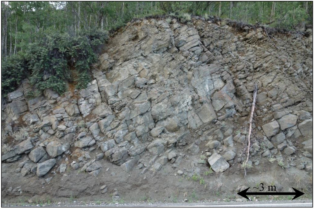
Figure 7.
Photograph of rock slope study Site A showing three well-defined discontinuity sets.
Figure 7.
Photograph of rock slope study Site A showing three well-defined discontinuity sets.
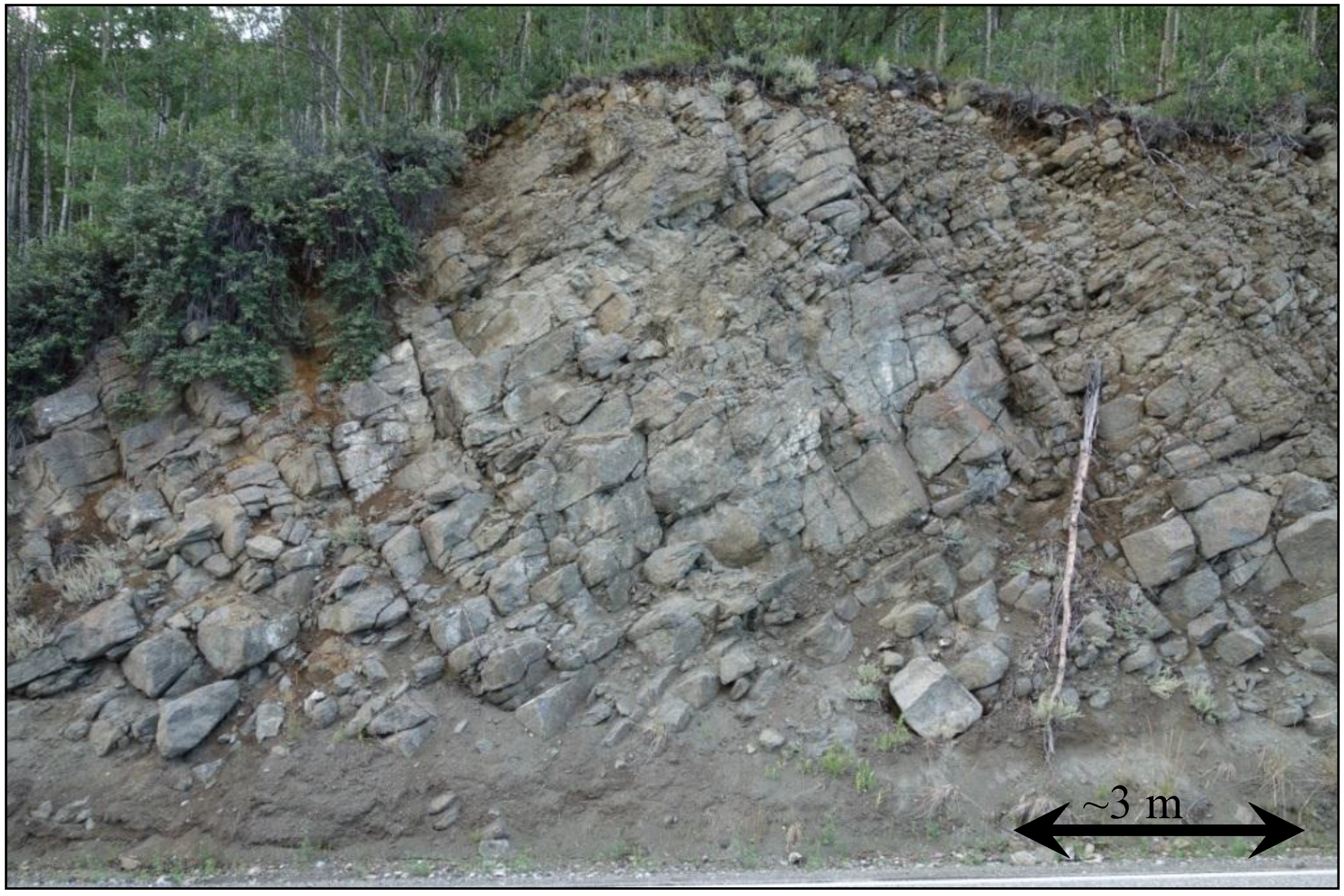

Figure 8.
Results from an approximately 35 m section of exposed rock at Site A (0.05 m cell size surface model from 2013).
Figure 8.
Results from an approximately 35 m section of exposed rock at Site A (0.05 m cell size surface model from 2013).
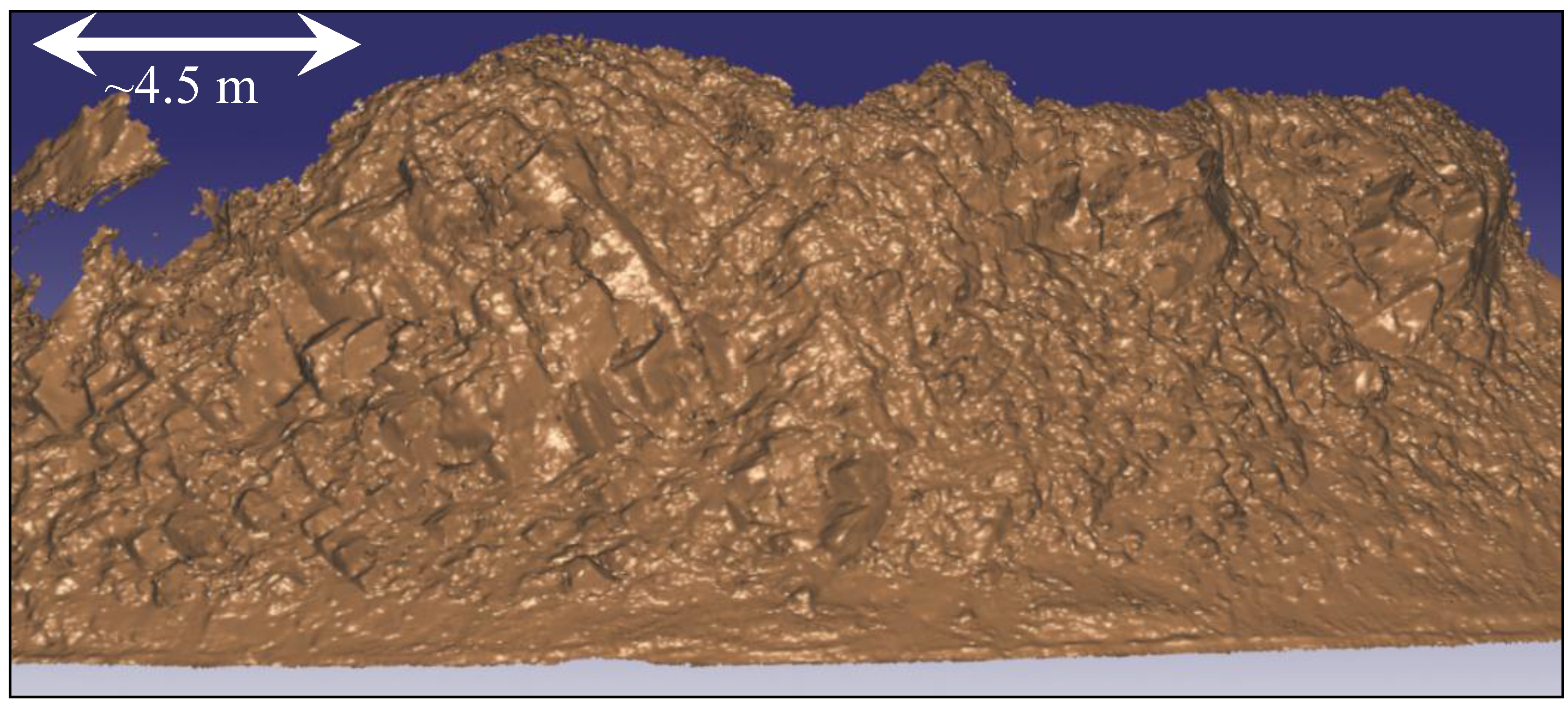
Figure 8 shows a sample triangulated shaded relief surface model with all holes filled for Site A. This model was generated with a 0.05 m cell size and adequately preserves the blocky rock mass features present across the slope. Analysis indicated that 13% (2014) to 15% (2013 data) of rock slope surface area was comprised of filled holes. Figure 9 shows the rockfall clustering results with resolutions ranging from 0.01–0.50 m without hole filling. As expected, the size of the change clusters increases for the coarser resolution models.

Figure 9.
Rockfall clustering results between 2013 and 2014 with varying model resolution including (A) 0.01 m; (B), 0.05 m; (C) 0.10 m; (D) 0.20 m; and (E) 0.50 m for Site A (90 m). The grey indicates portions of the cliff that did not experience significant erosional change. (Note that these sections may have experienced accretion). Larger white sections indicate holes or spacing between centroid points. Other colors represent a rock cluster where material has dislodged from the cliff. Each cluster is given an ID and colored based on that ID with a repeating pattern so that they can be distinguished from one another. For simplicity of rendering, the point cloud was used rather than the surface model.
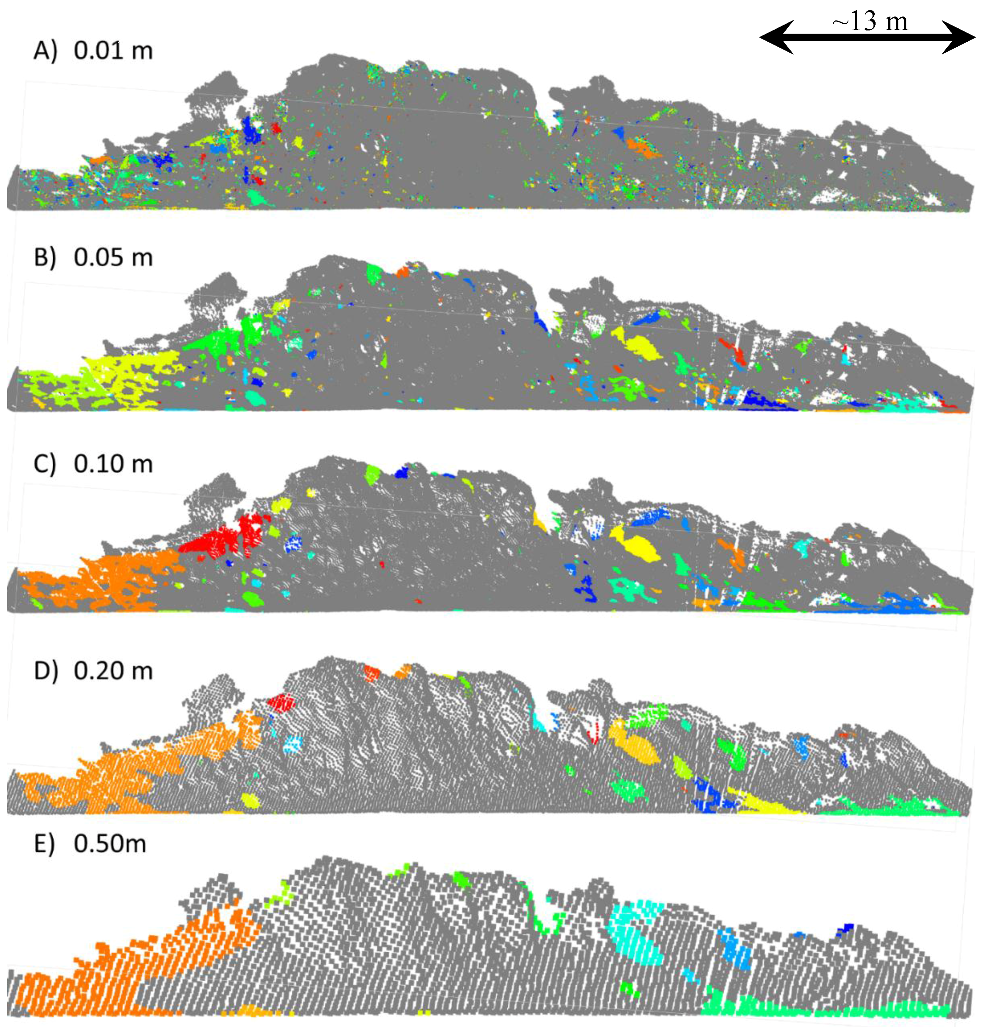
Figure 10 presents cumulative magnitude–frequency relationships derived from the clustering analysis of both the filled and unfilled models. The form of the magnitude–frequency relationships are similar to those derived for other rock slopes (e.g., [57,58]), and include characteristic “rollover” for small volumes as well as linearity in log-log space across several orders of magnitude of volume. The rollover phenomenon in landslide magnitude–frequency relationships has been attributed to data censuring that occurs when survey resolutions are approached [59]. The deviation from log-log linearity for large volumes has been noted by others (e.g., [57,58]) and attributed to the temporal censuring that occurs over relatively short monitoring time periods.

Figure 10.
Comparison of magnitude–frequency curves (plotted based on exceedance) for various resolutions and with hole filling (a, HF) and without hole filling (b, NHF) for Site A between 2013 and 2014.
Figure 10.
Comparison of magnitude–frequency curves (plotted based on exceedance) for various resolutions and with hole filling (a, HF) and without hole filling (b, NHF) for Site A between 2013 and 2014.
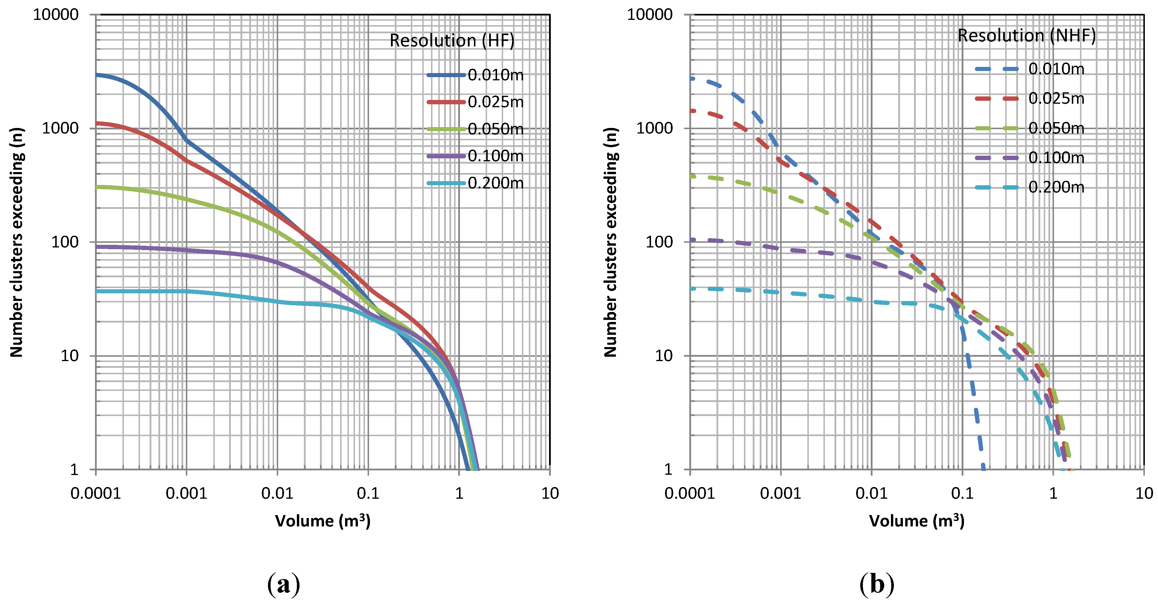
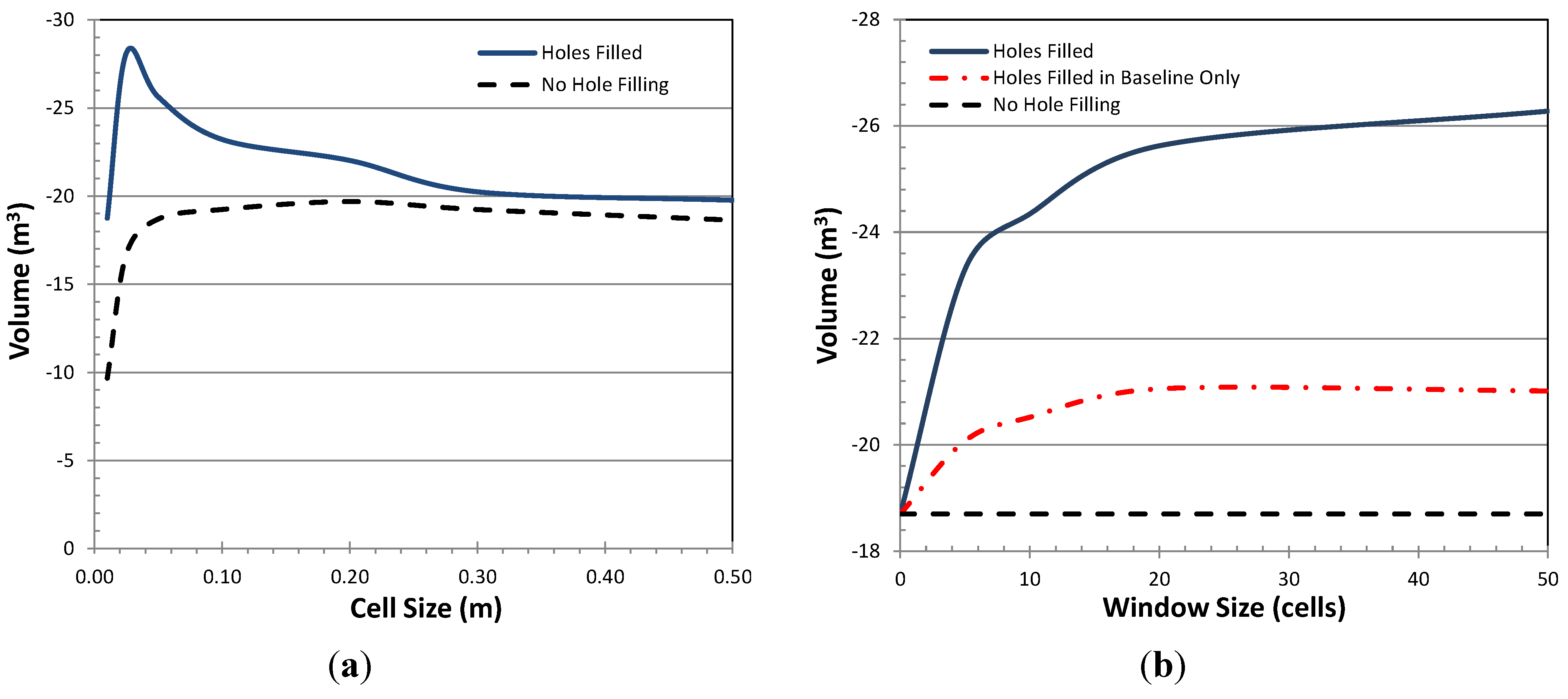
Figure 11a shows the estimated erosion volume calculated at different resolutions for models with and without hole filling. Note that for this analysis, hole filling window sizes varied with resolution and were selected such that small holes were filled, but larger holes that required excessive interpolation were not filled. The differences between erosion volumes calculated using models with holes filled versus those without hole filling generally increase as cell size decreases, and reach a maximum when the cell size equals ~0.025 m (the maximum feasible modeling resolution given the acquisition sampling of this dataset). The pronounced decrease in erosion volume (hole-filled model) that occurs for smaller cell sizes is attributed to survey resolution effects.
Figure 11b compares the influence of the search window size on the computed volumes considering holes filled in both models as well as considering those fill in the baseline model only. At small window dimensions, the computed volumes are highly sensitive to the size of the search window.
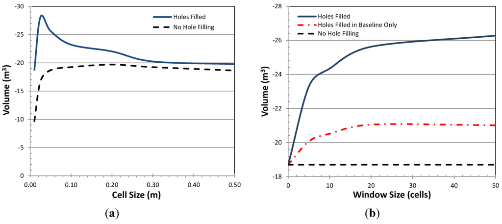
Figure 11.
(a) Comparison of calculated erosion volumes for various resolutions and with (HF) and without (NHF) hole filling for Site A between 2013 and 2014; (b) Comparison of rockfall volumes for Site A with varying hole filling search window size. Computations are based on a cell size of 0.05 m. The plateau indicates that the majority of the holes for Site A were small and filled with a window size of 15 cells (0.775 m).
3.2. Study Site B
Study Site B (Figure 12) is located along the Glenn Highway near milepost 87 and consists of an ~11 m high road cut, inclined at approximately 50 degrees. The exposed rock slope is approximately 110 m in length. The site includes soft argillaceous rocks (carbonaceous siltstones) of the Chickaloon formation that have been intruded by hard, well-indurated mafic sills (basalt) [56]. A major anti-dip (i.e., dipping into slope, with favorable structural control) discontinuity set is defined by the orientation of the contact with the intrusive basalt unit. This dominant set, along with other irregular joint sets in the sill material, produce rock fragments having maximum dimensions in the range of ~20 to ~200 cm. The significant contrast in strength between the siltstone and sill (basalt) materials has resulted in differential erosion features including cantilevered overhanging rocks. No seepage was observed during the fieldwork. Mass wasting along the lower portion of the slope occurs through erosion and raveling of the soft siltstone unit. Within the upper portion of the slope, mass wasting occurs both through release of rocks defined by discontinuities in the sill materials, as well as through tensile fracture and collapse of portions of the cantilevered sill rock.
Figure 13a shows a sample triangulated surface model with all holes filled (window size = 50 cells, or 2.5 m) for Site B. The model was generated with a 0.05 m cell size and effectively captures various overhanging features as well as abrupt transitions across the slope. Analysis indicated that 11% (2014) to 15% (2013 data) of rock slope surface area was comprised of holes. Figure 14 shows the rockfall clustering results with different window sizes for hole filling ranging from no holes filled to a window size of 50 cells (2.5 m).
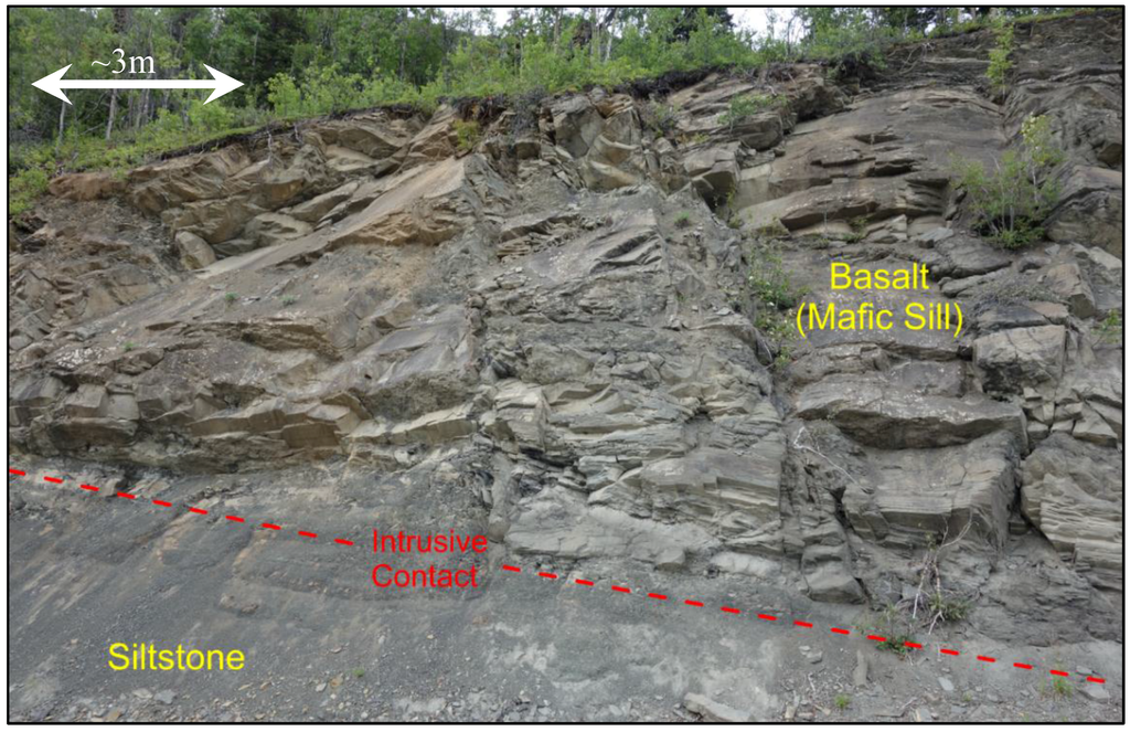
Figure 12.
Photograph of overhanging rock at Site B. The crest-to-toe vertical height of the slope is approximately 11 m.
Figure 12.
Photograph of overhanging rock at Site B. The crest-to-toe vertical height of the slope is approximately 11 m.


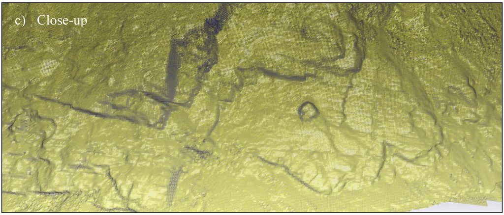
Figure 13.
Sample results of surface modeling (0.05 m resolution) from the 2014 survey of the exposed rock at Site B with holes filled for the (a) west and (b) east portions of the site; (c) Close-up wireframe model of a section for detail.
Figure 13.
Sample results of surface modeling (0.05 m resolution) from the 2014 survey of the exposed rock at Site B with holes filled for the (a) west and (b) east portions of the site; (c) Close-up wireframe model of a section for detail.
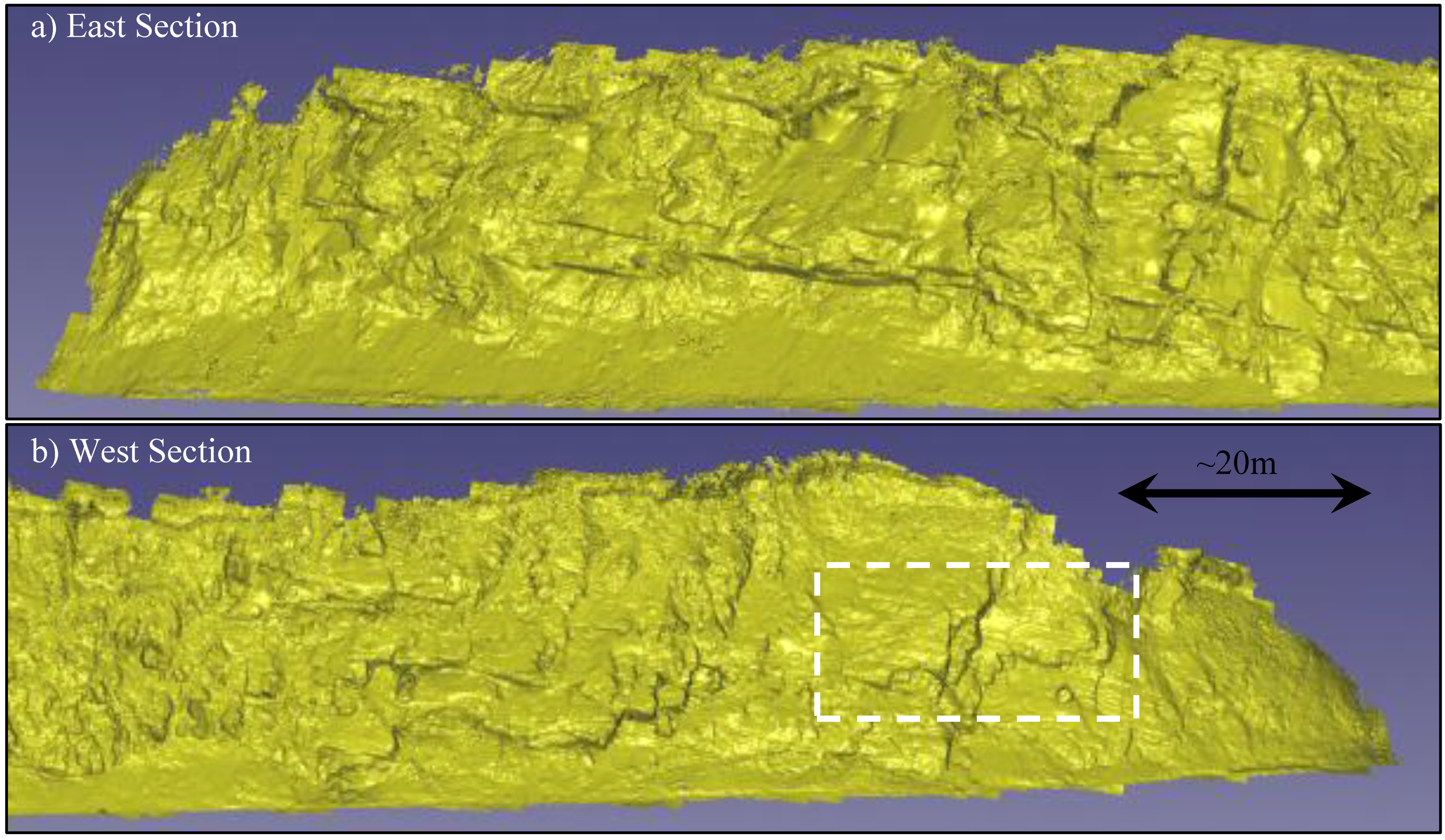

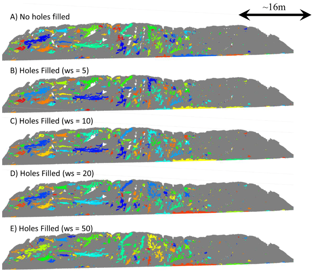
Figure 14.
Evaluation of the influence of varying the hole filling window size (ws) on the resulting rockfall clusters (2013–2014). Note that the figure uses the same coloring scheme as described in Figure 9 with grey representing areas of no significant erosion and white indicating holes in the dataset. For reference, this section is 110 m long. (A) no holes filled; (B) holes filled (ws = 5); (C) holes filled (ws = 10); (D) holes filled (ws = 20); (E) holes filled (ws = 50);

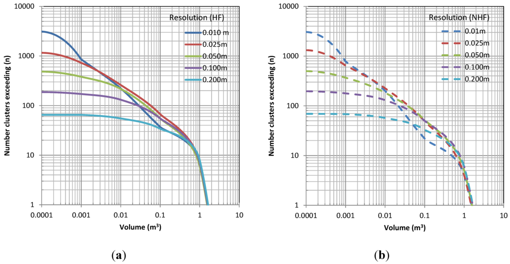
Figure 15.
Comparison of magnitude–frequency curves (plotted based on exceedance) for various resolutions and with (a, HF) and without (b, NHF) hole filling for Site B between 2013 and 2014.
Figure 15.
Comparison of magnitude–frequency curves (plotted based on exceedance) for various resolutions and with (a, HF) and without (b, NHF) hole filling for Site B between 2013 and 2014.
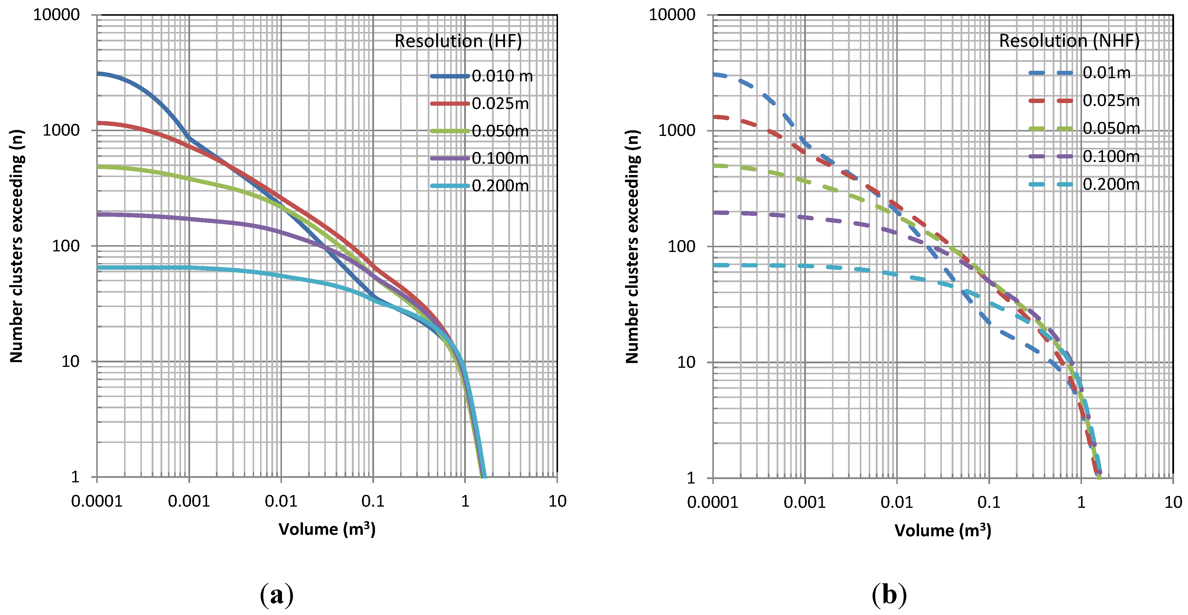
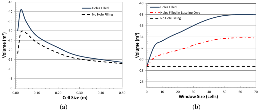
Figure 16.
(a) Comparison of calculated erosion volumes for various resolutions and with (HF) and without (NHF) hole filling for Site B between 2013 and 2014. Note that the hole filling window size was adjusted for each cell size analyzed such that it filled smaller holes, but did not fill excessively large holes; (b) Comparison of rockfall volumes for Site A with varying hole filling search window size. For this analysis, a constant cell size of 0.05 m was used. Note that at a window size of 50 (2.5 m), all holes are filled so the volume does not vary significantly below that.

Figure 15 shows the cumulative magnitude–frequency relationships derived from the clustering analysis of both filled and unfilled models. The form of the magnitude–frequency relationships are similar to those presented earlier for Site A. Figure 16a shows the estimated erosion volume calculated at different resolutions for models with and without hole filling. As with Site A, differences in erosion volume generally increase as cell size decreases. Figure 16b compares the influence of the search window size on the computed volumes considering holes filled in both models as well as considering those fill in the baseline model only.
3.3. Study Site C
Study Site C (Figure 17) is 340 m in length and located along the Parks Highway near milepost 239. It consists of a ~125 m-high road cut inclined at approximately 45 degrees. The site is situated within the Alaska Range, a mountain chain that extends west-to-east across southern Alaska, which creates a drainage divide between the Cook Inlet and the Yukon lowlands [60]. The seismically active Denali fault is located approximately 30 km south of the site. Rocks in the area generally consist of heavily metamorphosed schists and phylittes that have been intruded by large volcanic dikes at some locations [61]. They are highly weathered, medium strong muscovite-quartz and micaceous-quartz schist. This strongly foliated schist is highly anisotropic and includes widely spaced (~2 m), irregular joint sets. At one location at the site, the slope has been intruded by a steep trending volcanic dike. Seepage was not observed during the fieldwork, although concentrated surface flow was witnessed at several locations on the rock slope immediately following a major precipitation event. Mass wasting at the site occurs through a combination of erosion and raveling of soft materials along the surface of the slope, as well as through release of small to intermediate sized rocks (~10 to ~70 cm) leading to numerous rockfalls.
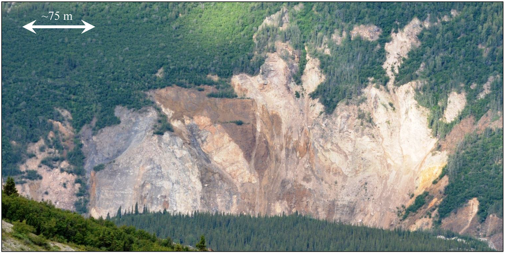
Figure 17.
Photograph of Site C. This photograph captures approximately 0.5 km of the slope along the highway. The highway and river are obscured by the lower trees.
Figure 17.
Photograph of Site C. This photograph captures approximately 0.5 km of the slope along the highway. The highway and river are obscured by the lower trees.

Several surface models were developed from the 2012 dataset (including both mobile and static lidar scans) and compared to reflectorless coordinates obtained across the slope using a total station. Table 3 summarizes the difference between total station coordinates and the derived surface models. Figure 18 shows the locations of those points as well as a sample model with 0.25 m resolution. Figure 19 shows the rockfall clustering results with different window sizes with no holes filled.
Figure 20 presents cumulative magnitude–frequency relationships derived from the clustering analysis of both filled and unfilled models, while Figure 21 presents the estimated erosion volume calculated at different resolutions for models with and without hole filling. These figures indicate that Site C generally exhibits trends that are comparable to Sites A and B, however, at a much larger magnitude.
Table 3.
Comparison of surface models and reflectorless total station coordinates scattered across the cliff face for the 2012 dataset.
| 3D Error Statistics (m) | Model Resolution | ||
|---|---|---|---|
| 10 cm * | 25 cm | 50 cm | |
| Minimum | −0.123 | −0.156 | −0.347 |
| Maximum | 0.091 | 0.119 | 0.161 |
| Average | −0.013 | −0.009 | −0.007 |
| Standard Deviation | 0.035 | 0.044 | 0.073 |
| Root Mean Square (RMS) | 0.037 | 0.045 | 0.074 |
| 3D Accuracy (95% Conf.) | 0.062 | 0.074 | 0.122 |
| Number of Samples | 50 * | 58 | 58 |
* Note that for the 10 cm model, the point density was too low on the upper cliff section to produce a satisfactory model for comparison with those points.

Figure 18.
Perspective view of the distribution of comparison points obtained with a total station to the 2012 surface model (25 cm resolution).
Figure 18.
Perspective view of the distribution of comparison points obtained with a total station to the 2012 surface model (25 cm resolution).
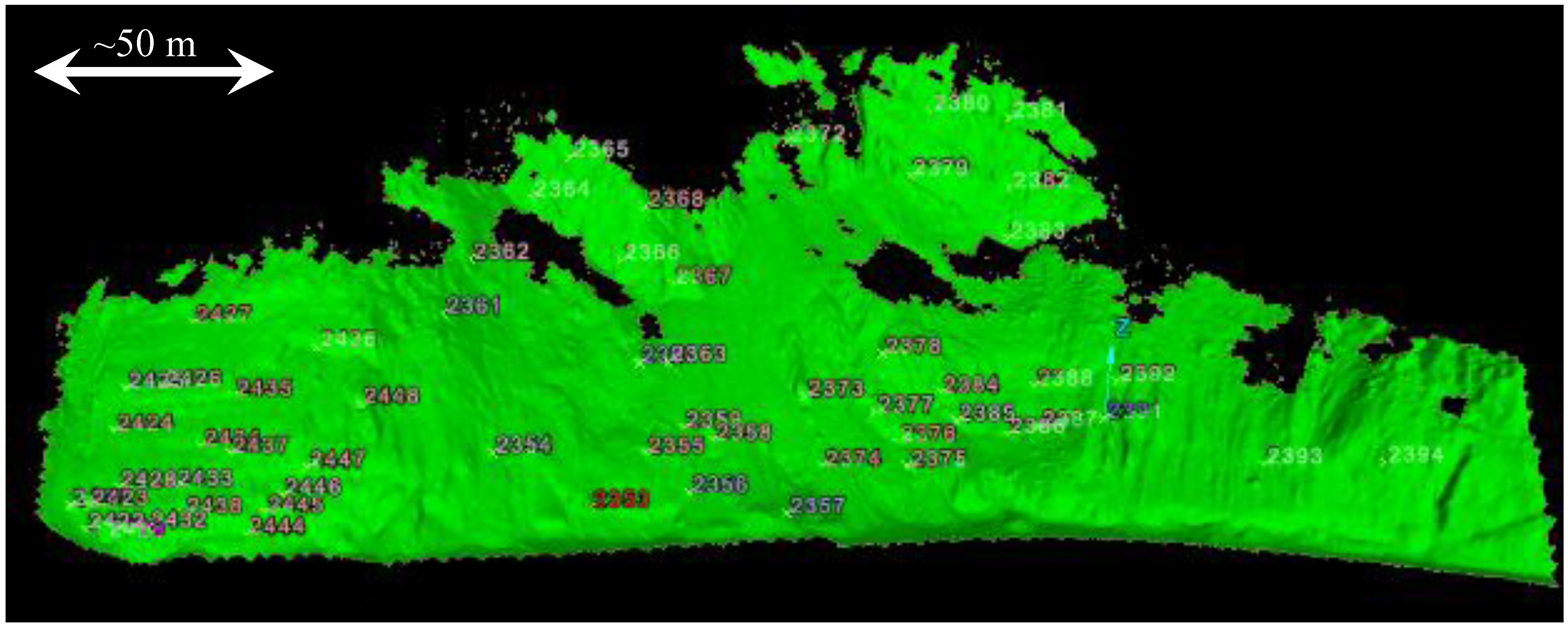

Figure 19.
Map of individual failure clusters between the 2013 and 2014 surveys at Site C (0.10 m resolution). These clusters are colored using the same scheme described in Figure 9 where grey indicates no significant erosion and white represents holes.
Figure 19.
Map of individual failure clusters between the 2013 and 2014 surveys at Site C (0.10 m resolution). These clusters are colored using the same scheme described in Figure 9 where grey indicates no significant erosion and white represents holes.
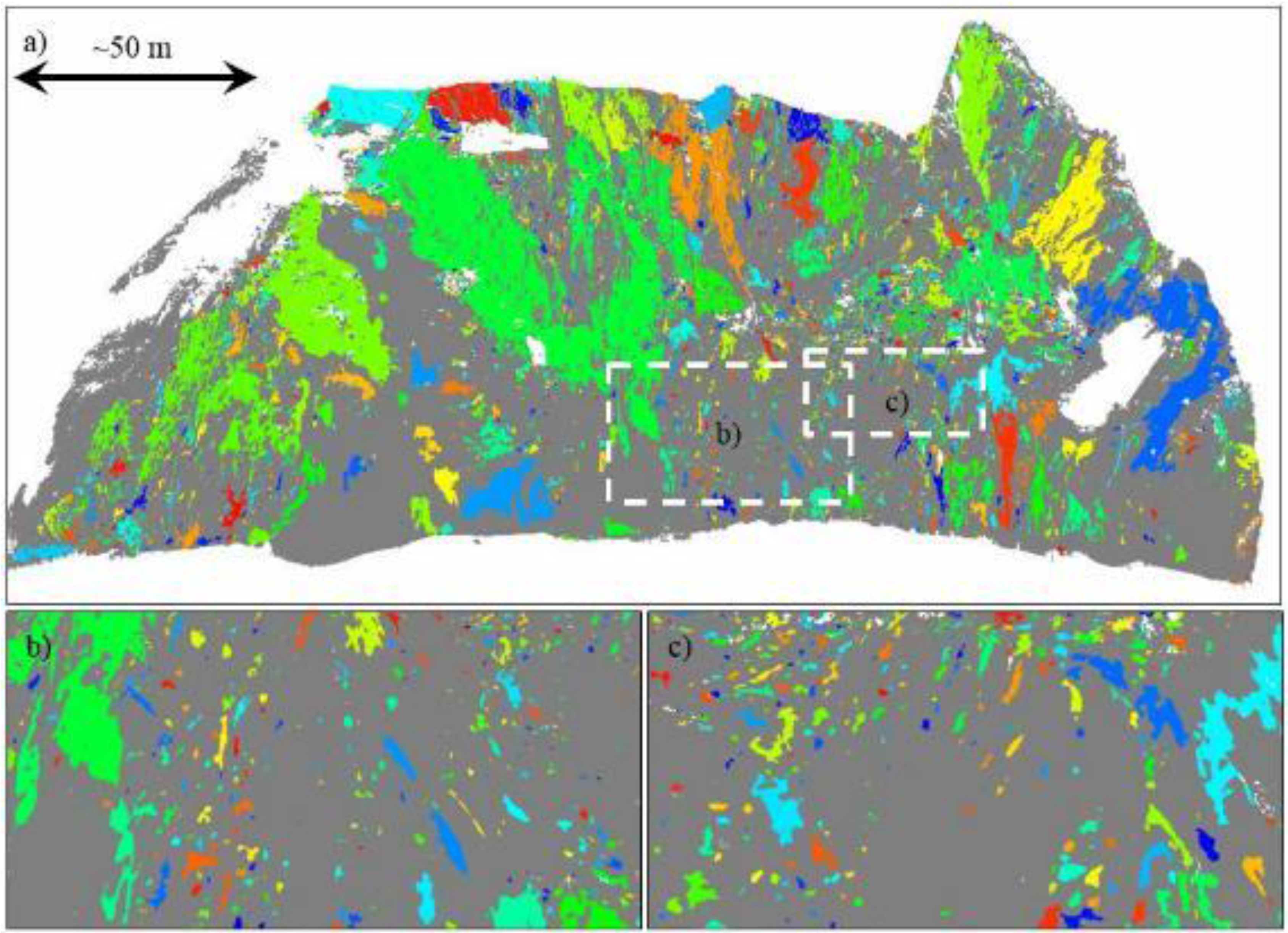
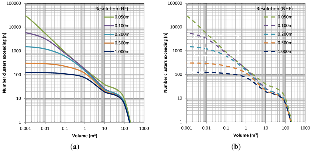
Figure 20.
Comparison of magnitude–frequency curves for various resolutions and with (a, HF) and without (b, NHF) hole filling between 2013 and 2014.
Figure 20.
Comparison of magnitude–frequency curves for various resolutions and with (a, HF) and without (b, NHF) hole filling between 2013 and 2014.

3.4. Comparison of Sites
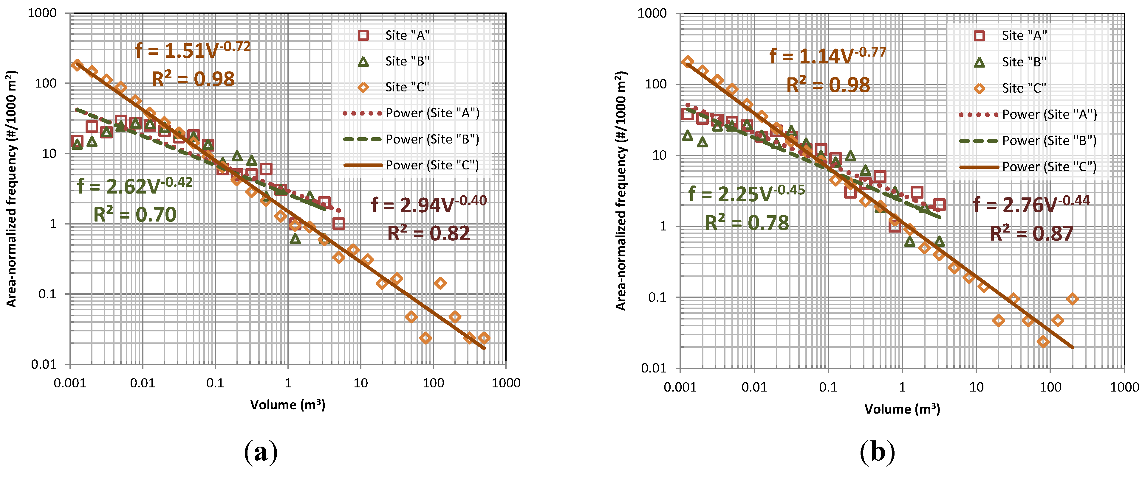
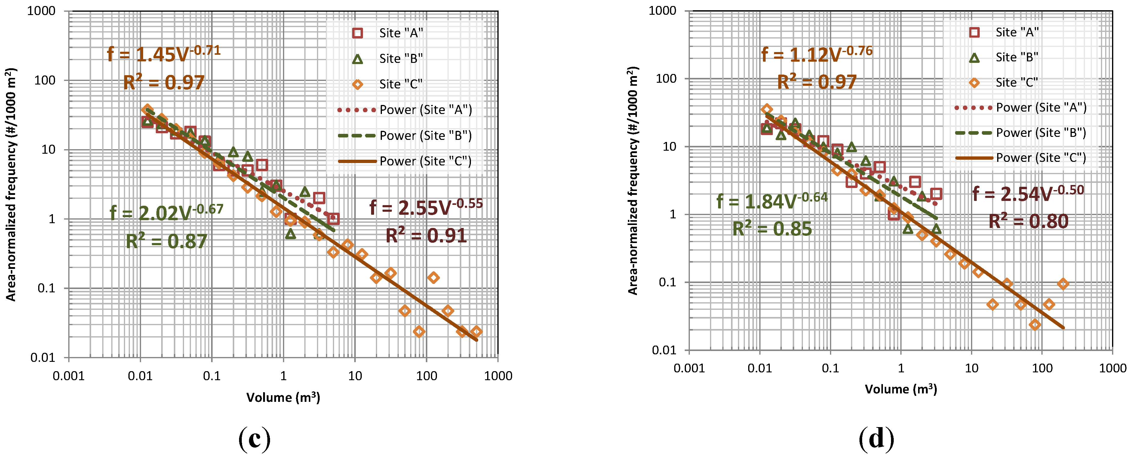
Figure 22 compares magnitude–frequency relationships for Sites A, B, and C. In contrast to the previous plots, which are presented as the number of events exceeding volumetric thresholds (i.e., cumulative plots), the relationships in Figure 22 were created by binning rockfall events based on equal increments (on a log scale) of volume to determine the frequency. Inverse power-law regressions were completed for each site considering only rockfall events >0.001 m3 (Figure 22a) and rockfall events >0.01 m3 (Figure 22b).
Because Site C is significantly longer than Sites A and B, the magnitude–frequency relationships for each site were normalized to an equivalent 1000 m2 section for the comparison. For this analysis, the 0.05 m resolution models with and without holes filled were utilized. The magnitude–frequency relationships shown in Figure 22 can be directly used in risk assessment of rock slopes (e.g., [57,58]).
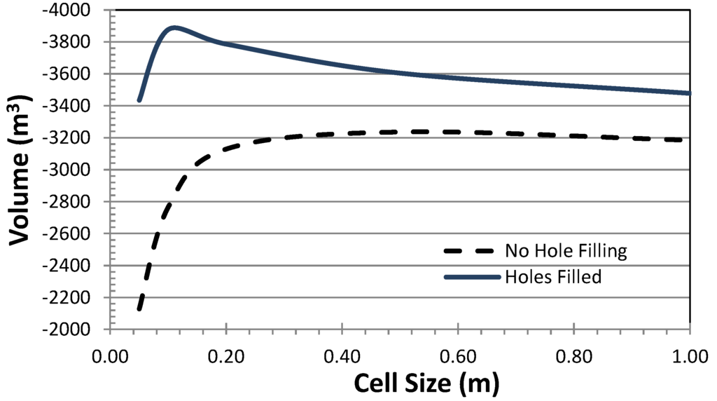
Figure 21.
Comparison of calculated erosion volumes for various resolutions and with (HF) and without (NHF) hole filling at site GG239 between 2013 and 2014.
Figure 21.
Comparison of calculated erosion volumes for various resolutions and with (HF) and without (NHF) hole filling at site GG239 between 2013 and 2014.
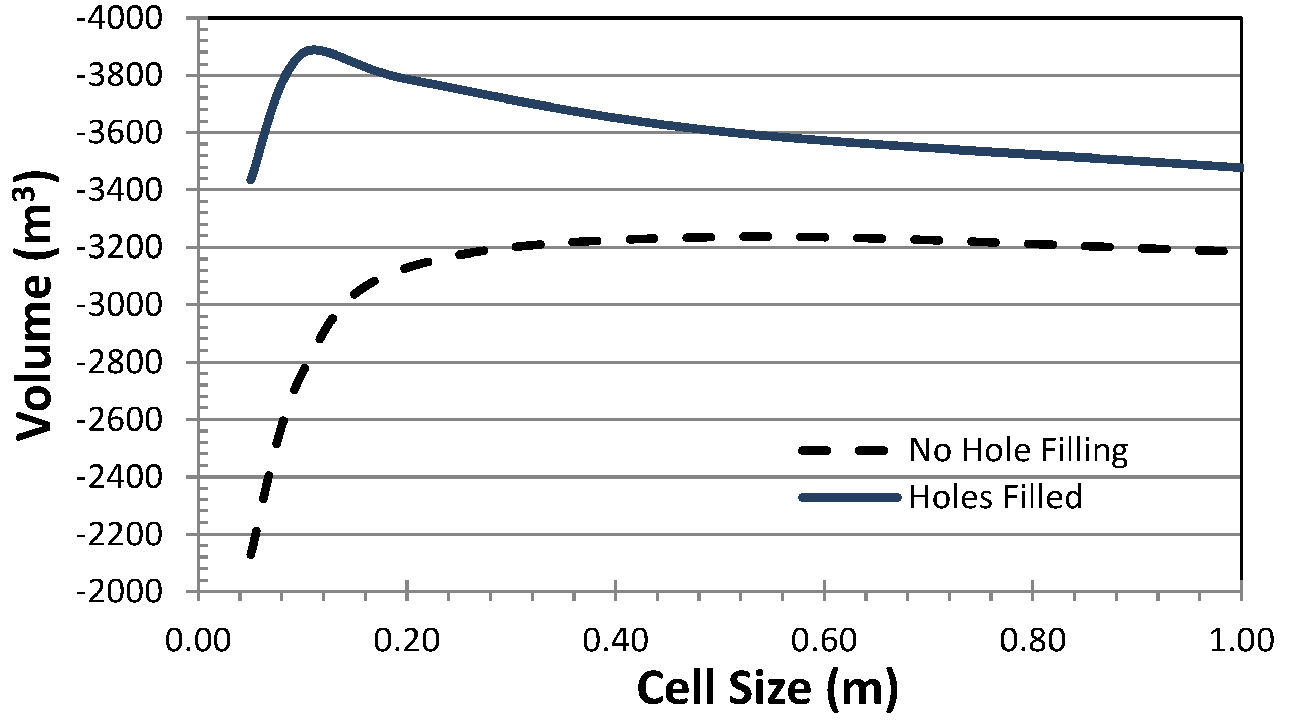
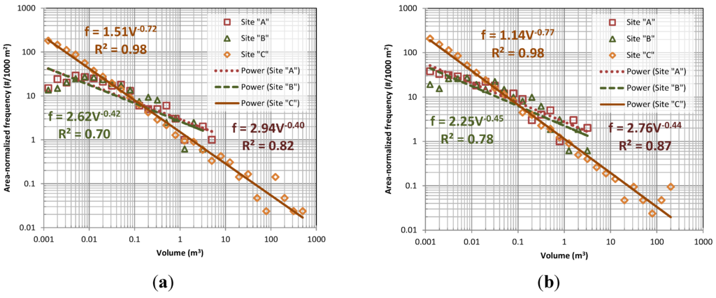

Figure 22.
Comparison of magnitude-frequency relationships (2013 to 2014, 0.05 cm holes filled models) and power law regressions for each site, normalized to an equivalent 1000 m2 area based on events >0.001 m3 (a) with and (b) without hole filling and events >0.01 m3 (c) with and (d) without hole filling.
4. Discussion
Sites A and B are located in a generally similar geologic setting, while Site C is located in distinctly different terrain. Despite the different settings, Figure 22 shows that, when normalized by area, all sites have similar magnitude–frequency relationships. Still, there is some variation observed between the sites. Perhaps most notably, Site C had significantly more events detected and a higher total volume of debris released during the observation period (~3 times higher debris volume when normalized by surface area). We attribute this to the marginal stability of Slope C, which was over-steepened during highway construction and today exhibits a very high rate of slope activity, evidenced by the need for frequent debris removal to maintain the catchment at the toe of the slope. In addition to generating a large volume of debris, Site C also produced a much wider range of rockfall fragment sizes, especially for larger volumes. We believe this is related to large slope height of the rock slope (~125 m), which allows large rock blocks to “daylight” and eventually fall from the slope. Sites A and B, in contrast, experienced fewer large volume failure events during the time period than expected based on the power law relationship. This may be a consequence of both the relatively short observation period (~1 year) and the relatively small slope heights (<10 m), which could impose kinematic constraints on large blocks within the rockmass. In either case, consideration of volume is important because rockfall runout distances generally increase with the mass of the debris being released [62]. Finally, it is worth noting that although the three sites exhibit generally similar normalized magnitude–frequency characteristics, from a practical perspective, Site C poses a much greater hazard to the highway simply because of its large rock face.
Comparison and detection of very small failures (<0.01 m3) remains a challenging task unless modeled at very high resolutions (e.g., 0.025 cm). For example, Figure 22 shows weaker inverse power law relationships when considering failures with volumes between 0.001 and 0.01 m3 for a 0.05 m model. At Sites A and B, these smaller events were not detected resulting in significant differences in power law regression fits. At Site C, in contrast, there is actually a slight improvement to the fit when considering these smaller events. This difficulty in detecting these small events occurs because:
- (1)
- Each scan is individually linked to GPS coordinates which have an accuracy of a few centimeters in ideal conditions,
- (2)
- Obtaining sufficient resolution and complete coverage across the entire cliff face to model such features is difficult, especially for tall or complex cliffs. While operators can control the desired angular resolution, there is always a tradeoff between the amount of coverage achievable and the desired level of detail (e.g., resolution). TLS systems do not capture resolution uniformly across the cliff surface due to the fact that it samples on angular increments, resulting in denser spacing close to the scanner and sparser further from the scanner. This wide distribution of sampling presents challenges when attempting to model the surface systematically for analysis.
- (3)
- There are noise present in each scan, which can be on the order of a few cm at oblique angles (e.g., [63]), or from small vegetation on the cliff surface that is difficult to remove, and
- (4)
- Holes will occur at different locations in the surveys at each epoch because it is very difficult to reoccupy the same positions when performing surveys of this scope.
Fortunately, smaller failure volumes (<0.01 m3) correspond to surface erosion (e.g., raveling), which does not pose a significant slope hazard and is typically neglected when assessing rock slope hazards. More rigorous field procedures and dense networks of targets could be implemented to enable improved detection of these failures at smaller individual sites as has been conducted in other studies, if needed; however, these techniques are not practical for long sections such as these because they are laborious to employ and also suffer from significant error propagation over large distances.
It also is difficult to isolate all individual rockfall events at highly active sites. For example, at Site C, many rockfall events were clustered together on some of the channel-like portions of the slope (i.e., “chutes,” Figure 19). To improve these results, surveys must be completed at higher temporal resolutions.
Model resolution plays a pivotal role in the volumes calculated as well as the magnitude–frequency relationships. Recall that in this study, resolution is defined in terms of the model resolution, rather than actual sampling resolution. Figure 11 and Figure 16 demonstrate that higher resolutions (lower cell size) are able to account for more erosion; however, the 0.01 m models underestimated the volume (Figure 11a and Figure 16a). Even with hole filling, the volume estimates for the 0.01 m models were markedly low because it is right at the typical acquisition resolution for Sites A and B. Note that although 0.01 m represents a typical sample spacing, there is significant variability in the actual spacing of the points due to sensor noise and topographic effects. Hence, there were insufficient cells with sample points to produce a satisfactory TPS (e.g., more than 50% of the cells in the window were required to have data), unless that criteria was relaxed. The 0.01 m models could also underestimate the volume because holes can be created in the rockfall scars themselves.
As the cell size increases, there are fewer holes and the volume estimates converge with those for the models where holes are not filled. Decreased resolution smoothes out smaller features on the surface (Figure 9), but also can help reduce noise in the surface that is present at higher resolutions due to the inability to remove short vegetation. This smoothing at lower resolution then effects the ability to detect change and results in smaller events being undetected (Figure 10a and Figure 15a). In turn, this leads to a lower estimated total volume at each site with decreased resolution (Figure 11a, Figure 16a, and Figure 21). Hence, the minimum detectable volume is primarily a function of resolution.
Figure 10, Figure 15 and Figure 20 all show significantly different magnitude–frequency relationships with varied resolution, particularly for detecting smaller volumes. Generally, the relationships are fairly similar for events greater than 0.1 m3. However, at Site A (Figure 10), the 0.01 m model without hole filling was unable to detect those larger events unless holes were filled. The 0.01 m model with holes filled produced a very similar magnitude–frequency relationship to the lower resolution models for volumes >0.01 m3. The 0.01 m model at Site B performed much better.
These smaller rockfall events cumulatively can be a significant portion of the total volumes. Sites A (Figure 11a) and C (Figure 21) were not very sensitive to model resolution for overall volume computations (except at high resolutions that resulted in significant data gaps). Site B, in contrast, showed higher dependence on resolution for the erosion volume computations (Figure 16a). This is because Site B contains several rock overhangs, which produce abrupt transitions in the terrain model. At this site, the resolution selected will significantly influence the ability to model those overhangs. Slight deviations in the models at rock overhangs between epochs result in overestimated change estimates because these overhangs are nearly perpendicular to the plane in which the data are modeled.
An additional comparison was made in Figure 11b and Figure 16b with filling holes in the baseline models only. There is a modest increase observed in volume estimates when holes are filled in the baseline surface as well as the model surface. While variance in the volumes is observed from the analysis based on modeling resolution, this variance is relatively small when considering the results from a highway risk assessment perspective (e.g., the difference between 20 and 28 m3 at Site A is insignificant when compared with the volume of 3900 m3 determined for Site C). Hence, the fluctuations in volume estimates across the resolution ranges are not as substantial as the natural variability that exists based on the rock structure across large spatial extents.
Nonetheless, hole filling by TPS works well for creating realistic surface and the models proved to be consistent with the topography. As evidenced in Figure 10, Figure 15, and Figure 20, there are relatively similar magnitude–frequency relationships for a given resolution whether holes were filled or not. However, hole filling clearly improved the ability to capture larger events that were sometimes split in the models without hole filling. The search window size should be set sufficiently large to ensure most holes are filled to avoid underestimating volumes (Figure 11b and Figure 16b); although, it should be recognized that a large search window will significantly increase computation time.
Interestingly, in Figure 14 the rockfall clustering results are similar with different levels of hole filling. Even when large holes were filled (e.g., ws = 50), the 2014 data matched the 2013 data well, as evidenced by the fact that many of those holes did not result in new artificial clusters being identified. This indicates that the TPS is reasonably estimating the surface, even when interpolating across these large holes. Indeed, the hole filling was important to better define the shapes and sizes of the existing clusters, particularly for grouping smaller clusters that were likely part of the same event.
In analyzing Figure 22, the power law magnitude–frequency relationships fit the data trends well across multiple orders of magnitude. However, the power law relationship tends to provide a weaker fit for smaller rockfalls (e.g., <0.01 m3 for sites A and B). Interestingly, for Site C, the predictive, power law magnitude–frequency relationship holds until considering volumes that are less than 0.0001 m3 (beyond what is shown in Figure 22). This threshold volume is essentially at the practical limits of the modeling (0.05 m) and survey techniques (0.05 m significant change threshold based on the estimated geo-referencing accuracy). In contrast, Sites A and B exhibit fewer small rockfalls than predicted based on the power law relationship. This may be due in part to censoring as survey resolutions are approached, but it also suggests that the hole filling method is not generating substantial artificial rockfalls. The correlation coefficients in Figure 22 indicate that hole filling generally leads to improved magnitude frequency fits as well (except for site B where hole filling reduces the effectiveness of capturing small failures). Still, it is possible that there may be some artificial rockfalls “detected” in the clustering analysis. Because of their small size, these smaller rockfalls are difficult to reliably verify with field or photographic techniques.
Overall, the clustering results for larger events compare well with a qualitative analysis of high-resolution photographs between epochs. Additionally, at Site A more rockfalls were detected on the west portion of the site than the east portion. The west portion was observed to be more active in field visits and tended to have substantially larger talus piles in the toe region adjacent to the roadway compared to the east portion of the site. Moreover, it is clear that the west portion is more actively eroding, evidenced by the presence of large, unstable overhangs, and increased surface roughness.
Change detection itself can be difficult when working with data sources of varying quality. For example, the 2012 mobile lidar dataset was coarser than the static TLS data, so it was difficult to compare. Reasonable models of a few centimeter resolutions were obtainable with TLS, but the MLS typically only supported models with resolutions coarser than 0.1 m. Within static scans, the change analysis results are improved if scans are acquired with similar resolutions and from similar vantage points as best as possible, so that holes occur on the same parts of the slope. Unfortunately, this can be difficult to do from a practical perspective for monitoring large sections, which was of interest in the overarching study.
5. Conclusions
Rock slopes pose costly and life threatening hazards in many parts of the world. TLS volumetric change analyses enables the development of relationships between rockfall volume (magnitude) and frequency of release (e.g., [57,58]) for risk assessment of these slopes. However, existing surface modeling methods can be difficult to employ, particularly on surfaces exhibiting significant morphologic complexity. In this paper, we present a new, fully automated approach to perform change detection and identify individual rockfalls on complex rock slopes. This new approach provides a streamlined method to analyze time series point clouds to isolate and quantify individual failure clusters (rockfall events) on the rock slope to generate magnitude–frequency relationships.
The approach was applied to several highly active, rock slope study sites in Alaska, U.S.A., resulting in magnitude–frequency relationships consistent with established theory (R2 > 0.7) at each site. The effects of hole filling and model resolution on the analysis were also evaluated. The TPS hole filling technique successfully created complete surface models that are fully consistent with the topography. The hole filling technique was also effective in capturing larger rockfall events that were erroneously separated into several smaller events using the traditional approach of not filling holes. The combined hole-filling and change-detection compared well with field observations and high-resolution photographic records from the study sites.
In general, model resolution plays a pivotal role in the ability to detect smaller rockfall events when developing magnitude–frequency relationships. The minimum detectable rockfall volume was found to be a function of the modeling resolution, assuming that sufficient resolution has been obtained during acquisition. The total volume estimates are also influenced by model resolution, but were comparatively less sensitive. In contrast, hole filling had a noticeable effect on magnitude–frequency relationships but to a lesser extent than modeling resolution. However, hole filling yielded a modest increase in overall volumetric quantity estimates.
Hence, it can be concluded that optimal results in estimating both magnitude–frequency relationships and volumetric quantities occur when appropriately balancing high modeling resolution with an appropriate level of hole filling.
Acknowledgments
Partial financial support for this project was provided by PacTrans and the Alaska Department of Transportation and Public Facilities. Leica Geosytems, and David Evans and Associates provided hardware, software, and field support for this study. Maptek I-Site provided software used for this study. We also thank Daniel Girardeau-Montaut and others who have developed the open source software CloudCompare, which was very useful for this project. We also utilized the open source GLC Player, developed by Laurent Ribon, for model visualization. OSU students John Raugust, Mahyar Sharifi-Mood, Jeremy Conner, and Rubini Santha assisted with the field data collection and processing. We appreciate the anonymous reviewers whose detailed comments, suggestions, and observations helped improve this manuscript significantly.
Author Contributions
Michael J. Olsen served as the lead author on the paper, developed the concept, methodology, and code as well as performed the analyses. Joseph Wartman supervised the field collection, provided the geologic background of the sites, verified the results with field and photographic surveys, and interpreted the data for the discussion. Martha McAlister aided with the data processing. Hamid Mahmoudabadi acquired the lidar data and assisted in the theoretical formulation for the methodology. Matt S. O’Banion acquired the lidar data, assisted with processing, and wrote code for the connected components algorithm. Lisa Dunham assisted with the geologic background research, performed testing on the code, and provided insights used to improve the algorithms. Keith Cunningham served as the Principal Investigator for the study. All authors contributed text, figures, and ideas throughout the manuscript.
Conflicts of Interest
The authors declare no conflict of interest.
References
- Petley, D. Global patterns of loss of life from landslides. Geology 2012. [Google Scholar] [CrossRef]
- Jaboyedoff, M.; Oppikofer, T.; Abellán, A.; Derron, M.H.; Loye, A.; Metzger, R.; Pedrazzini, A. Use of LIDAR in landslide investigations: A review. Nat. Hazards 2012, 61, 5–28. [Google Scholar] [CrossRef]
- Abellán, A.; Jaboyedoff, M.; Oppikofer, T.; Rosser, N.J.; Lim, M.; Lato, M. State of science: Terrestrial laser scanner on rock slopes instabilities. Earth Surf. Process. Landf. 2014, 39, 80–97. [Google Scholar] [CrossRef]
- Kemeny, J.; Turner, A.K. Ground-Based LiDAR Rock Slope Mapping and Assessment. Available online: http://zh.scribd.com/doc/85760902/GROUND-BASED-LiDAR-Rock-Slope-Mapping-and-Assessment#scribd (accessed on 31 May 2015).
- Girardeau-Montaut, D.; Roux, M.; Marc, R.; Thibault, G. Change detection on point cloud data acquired with a ground laser scanner. In Proceedings of the ISPRS Workshop Laser Scanning 2005, Enschede, the Netherlands, 12–14 September 2005.
- Teza, G.; Galgaro, A.; Zaltron, N.; Genevois, R. Terrestrial laser scanner to detect landslide displacement fields: A new approach. Int. J. Remote Sens. 2007, 28, 3425–3446. [Google Scholar] [CrossRef]
- Rabatel, A.; Deline, P.; Jaillet, S.; Ravanel, L. Rockfalls in high-alpine rock walls quantified by terrestrial lidar measurements: A case study in the Mont Blanc area. Geophys. Res. Lett. 2008, 35. [Google Scholar] [CrossRef]
- Alba, M.; Roncoroni, F.; Scaioni, M. Application of TLS for change detection in rock faces. In Proceedings of the ISPRS Laserscanning ‘09, Paris, France, 3–4 September 2009.
- Abellan, A.; Jaboyedoff, M.; Oppikofer, T.; Vilaplana, J.M. Detection of millimetric deformation using a terrestrial laser scanner: Experiment and application to a rockfall event. Nat. Hazards Earth Syst. Sci. 2009, 9, 365–372. [Google Scholar] [CrossRef]
- Abellán, A.; Calvet, J.; Vilaplana, J.M.; Blanchard, J. Detection and spatial prediction of rockfalls by means of terrestrial laser scanner monitoring. Geomorphology 2010, 119, 162–171. [Google Scholar] [CrossRef]
- Alba, M.; Scaioni, M. Automatic detection of changes and deformation in rock faces by terrestrial laser scanning. In Proceedings of the ISPRS Commission V Mid-Term Symposium, Newcastle upon Tyne, UK, 21–24 June 2010.
- Stock, G.M.; Luco, N.; Harp, E.L.; Collins, B.D.; Reichenbach, P.; Frankel, K.; Matasci, B.; Carrea, D.; Jaboyedoff, M.; Oppikofer, T. Quantitative rock-fall hazard and risk assessment for Yosemite Valley, California, in Landslides and Engineered Slopes: Protecting Society through Improved Understanding. In Proceedings of the 11th International Symposium on Landslides, Banff, AB, Canada, 3–8 June 2012.
- Collins, B.D.; Stock, G.M. Lidar Based Rock-Fall Hazard Characterization of Cliffs. Available online: http://www.nps.gov/yose/learn/nature/upload/Collins-Stock-2012-ASCE.pdf (accessed on 31 May 2015).
- Ravanel, L.; Deline, P.; Lambiel, C.; Vincent, C. Instability of a high alpine rock ridge: The lower Arête des Cosmiques, Mont Blanc Massif, France. Geogr. Ann. Ser. A Phys. Geogr. 2012. [Google Scholar] [CrossRef]
- Dewez, T.J.B.; Rohmer, J.; Regard, V.; Cnudde, C. Probabilistic coastal cliff collapse hazard from repeated terrestrial laser surveys: Case study from Mesnil Val (Normandy, northern France). J. Coast. Res. 2013, 65, 702–707. [Google Scholar]
- Lindenberg, R. Trends in detecting changes from repeated laser scanning data. In Proceedings of the 2nd Joint International Symposium on Deformation Monitoring, Nottingham, UK, 9–10 September 2013.
- D’Amato, J.; Guerin, A.; Hantz, D.; Rossetti, J.-P.; Jaboyedoff, M. Investigating rockfall frequency and failure configurations using Terrestrial Laser Scanner. In Proceedings of the IAEG XII Congress, Torino, Italy, 15–19 September 2014.
- Royan, M.J.; Abellán, A.; Jaboyedoff, M.; Vilaplana, J.M.; Calvet, J. Spatio-temporal analysis of rockfall pre-failure deformation using terrestrial LiDAR. Landslides 2013, 11, 697–709. [Google Scholar] [CrossRef]
- Girardeau-Montaut, D. Cloud Compare—3D Point Cloud and Mesh Processing Software. Available online: http://www.danielgm.net/cc/ (accessed on 19 April 2015).
- Olsen, M.J. In-situ change analysis and monitoring through terrestrial laser scanning. J. Comput. Civil Eng. 2015, 29, 04014040. [Google Scholar] [CrossRef]
- Lim, M.; Petley, D.N.; Rosser, N.J.; Allison, R.J.; Long, A.J.; Pybus, D. Combined digital photogrammetry and time-of-flight laser scanning for monitoring cliff evolution. Photogramm. Record 2005, 20, 109–129. [Google Scholar] [CrossRef]
- Lim, M.; Rosser, N.J.; Allison, R.J.; Petley, D. Erosional processes in the hard rock coastal cliffs at Staithes, North Yorkshire. Geomorphology 2010, 114, 12–21. [Google Scholar] [CrossRef]
- Lim, M.; Rosser, N.J.; Petley, D.N.; Keen, M. Quantifying the controls and influence of tide and wave impacts on coastal rock cliff erosion. J. Coast. Res. 2011, 27, 46–56. [Google Scholar] [CrossRef]
- Rosser, N.J.; Dunning, S.A.; Lim, M.; Petley, D.N. Terrestrial laser scanning for quantitative rock fall hazard assessment. Landslides 2007, 10, 409–420. [Google Scholar]
- Rosser, N.J.; Lim, M.; Petley, D.N.; Dunning, S.; Allison, R.J. Patterns of precursory rockfall prior to slope failure. J. Geophys. Res. 2007, 112. [Google Scholar] [CrossRef]
- Rosser, N.J.; Petley, D.N.; Lim, M.; Dunning, S.A.; Allison, R.J. Terrestrial laser scanning for monitoring the process of hard rock coastal cliff erosion. Q. J. Eng. Geol. Hydrogeol. 2005, 38, 363–375. [Google Scholar] [CrossRef]
- Olsen, M.J.; Johnstone, E.; Driscoll, N.; Ashford, S.A.; Kuester, F. Terrestrial laser scanning of extended cliff sections in dynamic environments: A parameter analysis. J. Surv. Eng. 2009, 135, 161–169. [Google Scholar] [CrossRef]
- Lato, M.; Hutchinson, J.; Diederichs, M.; Ball, D.; Harrap, R. Engineering monitoring of rockfall hazards along transportation corridors: Using mobile terrestrial LiDAR. Nat. Hazards Earth Syst. Sci. 2009, 9, 935–946. [Google Scholar] [CrossRef]
- Barlow, J.; Lim, M.; Rosser, N.J.; Petley, D.N.; Brain, M.J.; Norman, E.C.; Geer, M. Modeling cliff erosion using negative power law scaling of rockfalls. Geomorphology 2012, 139–140, 416–424. [Google Scholar] [CrossRef]
- Olsen, M.J.; Chen, Z.; Hutchinson, T.C.; Kuester, F. Optical techniques for multi-scale damage assessment in natural hazard analysis. Geomat. Nat. Hazards Risk 2013, 4, 49–70. [Google Scholar] [CrossRef]
- Santana, D.; Corominas, J.; Mavrouli, O.; Garcia-Sellés, D. Magnitude–frequency relation for rockfall scars using a terrestrial laser scanner. Eng. Geol. 2012, 145–146, 50–64. [Google Scholar] [CrossRef]
- Lee, M.L.; Jones, K.C. Landslide Risk Assessment; ICE Publishing: London, UK, 2014. [Google Scholar]
- Tonini, M.; Abellán, A. Rockfall detection from LiDAR point clouds: A clustering approach using R. J. Spat. Inf. Sci. 2014, 8, 95–110. [Google Scholar] [CrossRef]
- Carrea, D.; Abellán, A.; Derron, M.H.; Jaboyedoff, M. Automatic rockfalls volume estimation based on terrestrial laser scanning data. Eng. Geol. Soc. Territ. 2015, 2, 425–428. [Google Scholar]
- Turk, G.; Levoy, M. Zippered polygon meshes from range images. In Proceedings of the 21st Annual Conference on Computer Graphics and Interactive Techniques, Orlando, FL, USA, 24–29 July 1994; pp. 311–318.
- Bernardini, F.; Mittleman, J.; Rushmeier, H.; Silva, C.; Taubin, G. The ball-pivoting algorithm for surface reconstruction. IEEE Trans. Vis. Comput. Graph. 1999, 5, 349–359. [Google Scholar] [CrossRef]
- Bernardini, F.; Martin, I.; Mittleman, J.; Rushmeier, H.; Taubin, G. Building a digital model of michelangelo’s florentine pieta. IEEE Comput. Graph. Appl. 2002, 22, 59–67. [Google Scholar] [CrossRef]
- Medeiros, E.; Velho, L.; Lopes, H. A topological framework for advancing front triangulation. In Proceedings of the XVI Brazilian Symposium on Computer Graphics and Image Processing (SIBGRAPI′03), Sao Carlos, Brazil, 12–15 October 2003.
- Sheng, L.; Li-qu, L.; Xiao-main, C. A new mesh growing surface reconstruction algorithm. In Proceedings of the First International Workshop on Education Technology and Computer Science (ETCS), Wuhan, Hubei, 7–8 March 2009; Volume 3, pp. 889–893.
- Olsen, M.J.; Johnstone, E.; Kuester, F. Hinged, pseudo-grid triangulation method for long, near linear cliff analysis. J. Surv. Eng. 2013, 139, 105–109. [Google Scholar] [CrossRef]
- National Geodetic Survey. OPUS: Online Positioning User Service. Available online: http://www.ngs.noaa.gov/OPUS/ (accessed on 24 August 2015).
- Olsen, M.J.; Johnstone, E.; Kuester, F.; Ashford, S.A.; Driscoll, N. New automated point-cloud alignment for ground based lidar data of long coastal sections. J. Surv. Eng. 2011, 137, 14–25. [Google Scholar] [CrossRef]
- Williams, K.; Olsen, M.J.; Chin, A. Accuracy assessment of geo-referencing methodologies for terrestrial laser scan surveys. In Proceedings of the ASPRS Annual Conference, Sacramento, CA, USA, 19–23 March 2012.
- Silvia, E.P.; Olsen, M.J. To Level or Not to Level: Laser scan inclination sensor evaluation. J. Surv. Eng. 2012, 138, 117–125. [Google Scholar] [CrossRef]
- Eberly, D. Least Squares Fitting of Data, Geometric Tools, LLC. Available online: http://www.geometrictools.com (accessed on 17 April 2015).
- Horn, B.K.P. Closed-Form solution of absolute orientation using unit quaternions. J. Opt. Soc. Am. 1987, 4, 629–642. [Google Scholar] [CrossRef]
- Horn, B.K.P.; Hilden, H.; Negahdaripour, S. Closed-Form solution of absolute orientation using orthonormal matricies. J. Opt. Soc. Am. 1988, 5, 1127–1135. [Google Scholar] [CrossRef]
- Donato, G.; Belongie, S. Approximation Methods for Thin Plate Spline Mappings and Principal Warps. Available online: http://cseweb.ucsd.edu/~sjb/pami_tps.pdf (accessed on 31 May 2015).
- Elonen, J. Thin Plate Spline Editor—An Example Program in C++. Available online: http://elonen.iki.fi/code/tpsdemo/ (accessed on 17 April 2015).
- Szeliski, R. Computer Vision: Algorithms and Applications; Springer Press: Berlin, Germany, 2011. [Google Scholar]
- Barnhart, T.B.; Crosby, B.T. Comparing two methods of surface change detection on an evolving thermokarst using high-temporal-frequency terrestrial laser scanning, Selawik River, Alaska. Remote Sens. 2013, 5, 2813–2837. [Google Scholar] [CrossRef]
- Zeiback, R.; Filin, S. Change detection via terrestrial laser scanning. In Proceedings of the Laser Scanning 2007 and SilviLaser 2007, ISPRS, Espoo, Finland, 12–14 September 2007; pp. 430–435.
- Dillencourt, M.B.; Samet, H.; Tamminen, M. A general approach to connected-component labeling for arbitrary image representations. J. ACM 1992, 39, 253–280. [Google Scholar] [CrossRef]
- Fisher, R.; Perkins, S.; Walker, A.; Wolfart, E. Connected Components Labeling. Available online: http://homepages.inf.ed.ac.uk/rbf/HIPR2/label.htm (accessed on 20 April 2015).
- Plafker, G.; Berg, H.C. The Geology of Alaska; Geologic Society of America: Boulder, CO, USA, 1994. [Google Scholar]
- Trop, J.M.; Plawman, T.L. Bedrock Geology of the Glenn Highway from Anchorage to Sheep Mountain, Alaska: Mesozoic-Cenozoic Forearc Basin Development along an Accretionary Convergent Margin. Available online: http://archives.datapages.com/data/alaska/data/029/029001/1_akgs0290001.htm (accessed on 31 May 2015).
- Hungr, O.; Evans, S.G.; Hazzard, J. Magnitude and frequency of rock slides along the main transportation corridors of southwestern British Columbia. Can. Geotech. J. 1999, 36, 224–238. [Google Scholar] [CrossRef]
- Hantz, D. Quantitative assessment of diffuse rock fall hazard along a cliff foot. Nat. Hazards Earth Syst. Sci. 2011, 11, 1303–1309. [Google Scholar] [CrossRef]
- Guzzetti, F.; Malamud, B.D.; Turcotte, D.L.; Reichenbach, P. Power-law correlations of landslide areas in central Italy. Earth Planet. Sci. Lett. 2002, 195, 169–183. [Google Scholar] [CrossRef]
- National Parks Service. Thornberry-Ehrlich, Denali National Park and Preserve: Geologic Resources Inventory Report; National Parks Service: Denver, CO, USA, 2010. [Google Scholar]
- Wahrhaftig, C.; Black, R.F. Engineering Geology along Part of the Alaska Railroad; U.S. Geological Survey: Reston, VA, USA, 1958.
- Turner, A.; Duffy, J.D. Modeling and Prediction of Rockfall, Rockfall Characterization and Control; Turner, A., Schuster, R., Eds.; Transportation Research Board: Washington, DC, USA, 2012. [Google Scholar]
- Lichti, D.; Gordon, S.; Tipdecho, T. Error models and propagation in directly georeferenced terrestrial laser scanner networks. J. Surv. Eng. 2005, 131, 135–142. [Google Scholar] [CrossRef]
© 2015 by the authors; licensee MDPI, Basel, Switzerland. This article is an open access article distributed under the terms and conditions of the Creative Commons Attribution license (http://creativecommons.org/licenses/by/4.0/).