An Evaluation of Different Training Sample Allocation Schemes for Discrete and Continuous Land Cover Classification Using Decision Tree-Based Algorithms

Abstract

Land cover mapping for large regions often employs satellite images of medium to coarse spatial resolution, which complicates mapping of discrete classes. Class memberships, which estimate the proportion of each class for every pixel, have been suggested as an alternative. This paper compares different strategies of training data allocation for discrete and continuous land cover mapping using classification and regression tree algorithms. In addition to measures of discrete and continuous map accuracy the correct estimation of the area is another important criteria. A subset of the 30 m national land cover dataset of 2006 (NLCD2006) of the United States was used as reference set to classify NADIR BRDF-adjusted surface reflectance time series of MODIS at 900 m spatial resolution. Results show that sampling of heterogeneous pixels and sample allocation according to the expected area of each class is best for classification trees. Regression trees for continuous land cover mapping should be trained with random allocation, and predictions should be normalized with a linear scaling function to correctly estimate the total area. From the tested algorithms random forest classification yields lower errors than boosted trees of C5.0, and Cubist shows higher accuracies than random forest regression.

1. Introduction

Land cover classification from satellite images is one of the primary fields in remote sensing. Finer spatial resolution data (10–30 m), in particular from Landsat, has been widely used for regional studies of land cover and change, and very fine spatial resolution imagery (<1 to 5 m) play an important role in local studies. Wall-to-wall mapping of large areas with 10–30 m data is expensive in terms of financial and computational resources, and there are only a few efforts for large areas, such as the National Land Cover Dataset (NLCD) of the United States [1], the National Land Cover of South Africa (NLC) [2], or the European Coordination of Information on the Environment as pan-European maps (CORINE) [3]. Recently, global forest cover [4,5] and global land cover maps [6] were derived from 30 m Landsat data. Most macro-regional, continental, and global applications, however, employ data of relatively coarse spatial resolution (250–1000 m) from Terra-Aqua/MODIS, SPOT/VEGETATION, NOAA/AVHRR, and ENVISAT/MERIS. Besides fewer difficulties in handling data volumes, the increased number of available cloud-free images allows for generation of data composites, and the dense temporal information helps to discern classes by their distinct phenological patterns. The latter is advantageous for mapping across various ecoregions where classes are likely to be represented by multiple clusters in feature space [7,8].

The lack of spatial detail of coarse resolution data imposes limitations for accurate land cover characterization [9,10,11]. The assignment of discrete classes to coarse resolution cells cannot adequately describe spatially complex areas [12]. The likelihood for mixed pixels is a function of the spatial resolution, the thematic detail to be mapped, and the size and spatial pattern of land cover patches [13]. However, discrete class assignment of mixed pixels not only imposes serious difficulties to coarse image data classification but also alters the area estimation. Several studies have noted that at coarser spatial resolution dominating classes with large patches yield higher area proportions than expected at the expense of dispersed, small-patch classes [7,13,14]. Studies have postulated that area calculations from fractional estimates are more accurate than from discrete classifications [7,15].

Several algorithms have been explored for large area mapping with coarse resolution data. For instance, Fernandes et al. [10] compared a hard classifier, artificial neural networks (ANN), linear spectral unmixing, clustering, and linear regression for fractional class estimation and found differences of approximately 20% compared to fine resolution reference data. Studies focusing on urban land cover compared advanced regression algorithms [16] or various discrete classifiers [17]. Several studies for the same global 1° spatial resolution AVHRR Normalized Difference Vegetation Index (NDVI) dataset have shown that classification of 11 land cover classes with decision trees (DT) perform best with 93% overall accuracy [18] compared to Maximum Likelihood classification (78%) [19] and ANN (85%) [20]. Most automated processing systems for macro-regional to global land cover characterization employ DT approaches [1,12,21,22,23,24,25]. There are two general types of DT: classification trees (CT) with a discrete target value and regression trees (RT) with a continuous result.

Besides the classification algorithm, features and training data for supervised image classification have to be defined. Several studies address feature generation and selection processes [26,27,28,29] and various aspects of training data selection [17,30,31,32]. However, only a few studies have focused on training data allocation schemes, such as between-class sample balance or the structure of heterogeneous samples. In particular classification trees may suffer from an unbalanced sample size between classes because the number of samples in each leaf defines the class [33,34], and several allocation schemes have been recommended [24,26,27,32]. A few studies recommend heterogeneous training data for discrete classification [35,36] but most large-area mapping projects select homogeneous areas for training [7,22,27]. For regression techniques, the impact of non-random selection of heterogeneous training data is unknown, and the impact of combined tree models for several classes on correct area estimation has been widely overlooked.

The objective of this study is to compare the accuracy and area estimations of several decision tree approaches trained with specific sample allocation schemes from an existing higher spatial resolution map for discrete and continuous land cover mapping. Specific goals are:

(1).

Evaluate the performance of DT algorithms using two common approaches of classification and regression trees

(2).

For classification trees, compare (a) heterogeneous training pixels with different allocation schemes against homogeneous pixels and (b) schemes of sample allocation between classes

(3).

For regression trees, assess (a) sample allocations for heterogeneous samples and (b) normalized and non-normalized results to combine multiple models.

2. Data and Study Area

2.1. National Land Cover Data of the United States from Landsat Images

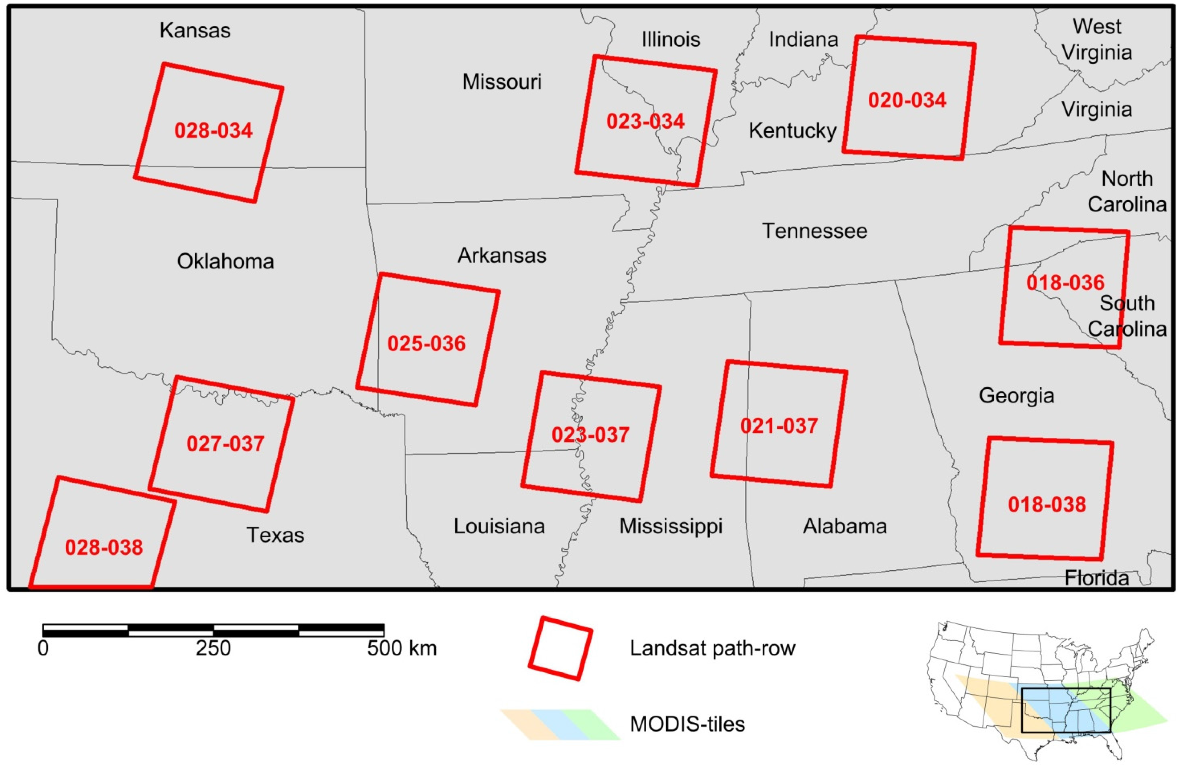
The National Land Cover Data set (NLCD) of the United States is a 30 m Landsat TM/ETM⁺-based classification with 16 classes produced by the United States Geological Survey (USGS). There are two maps (1992, 2001) [1] and map updates for 2006 and 2011 [37,38,39]; the 2006 update was used in this study. NLCD2006 has an overall accuracy of 78% [40] and a small class-specific minimum mapping unit [37]. NLCD data are provided in Albers Equal Area (AEA) projection with NAD83 datum, standard parallels at 23.5°N and 45.5°N, and an origin of latitude and longitude at 23°N and 96°W, which is also the map projection of this study. In this study, a subset of 60,000 × 30,000 pixels, extending from western Kansas (101°W, 39°N) to Jacksonville, FL (80°W, 30°N), was extracted (see Figure 1). In addition, ten Landsat images (Figure 1) were downloaded for accuracy assessment and evaluation of spatial co-registration between MODIS and Landsat from which NLCD2006 was derived.

2.2. MODIS Data

The MODIS nadir bidirectional reflectance distribution function (BRDF)-adjusted surface reflectance (NBAR) product with 926.6 m spatial resolution (MCD43B4) and the corresponding quality assessment science dataset (MCD43B2) were downloaded from the Land Processes Distributed Active Archive Center (LP DAAC) for the period of October 2005 to March 2007. The NBAR product applies the BRDF parameters to cloud-free and atmospherically corrected surface reflectance data (bands 1 to 7) with a solar angle at local solar noontime. This mimics a nadir-viewing instrument and results in a stable and consistent dataset [41,42]. MCD43 products combine images of Terra and Aqua acquisitions over a 16-day period but are produced every eight days by rolling compositing. Three tiles (h09v05, h10v05, h11v05; Figure 1) were mosaicked, resampled to 900 m using nearest neighbor (NN) resampling, subset to 2000 × 1000 pixels, and projected to the AEA projection with projection parameters equal to NLCD. The cell size of 900 m, as compared to the more commonly used 1000 m, was chosen to nest the grid with 30 m cells from NLCD; thus a block of 30 × 30 cells of NLCD2006 corresponds to one MODIS cell at 900 m.

Figure 1. Study area in the southeastern United States, showing MODIS tiles and Landsat path-rows.

Figure 1. Study area in the southeastern United States, showing MODIS tiles and Landsat path-rows.

3. Methods

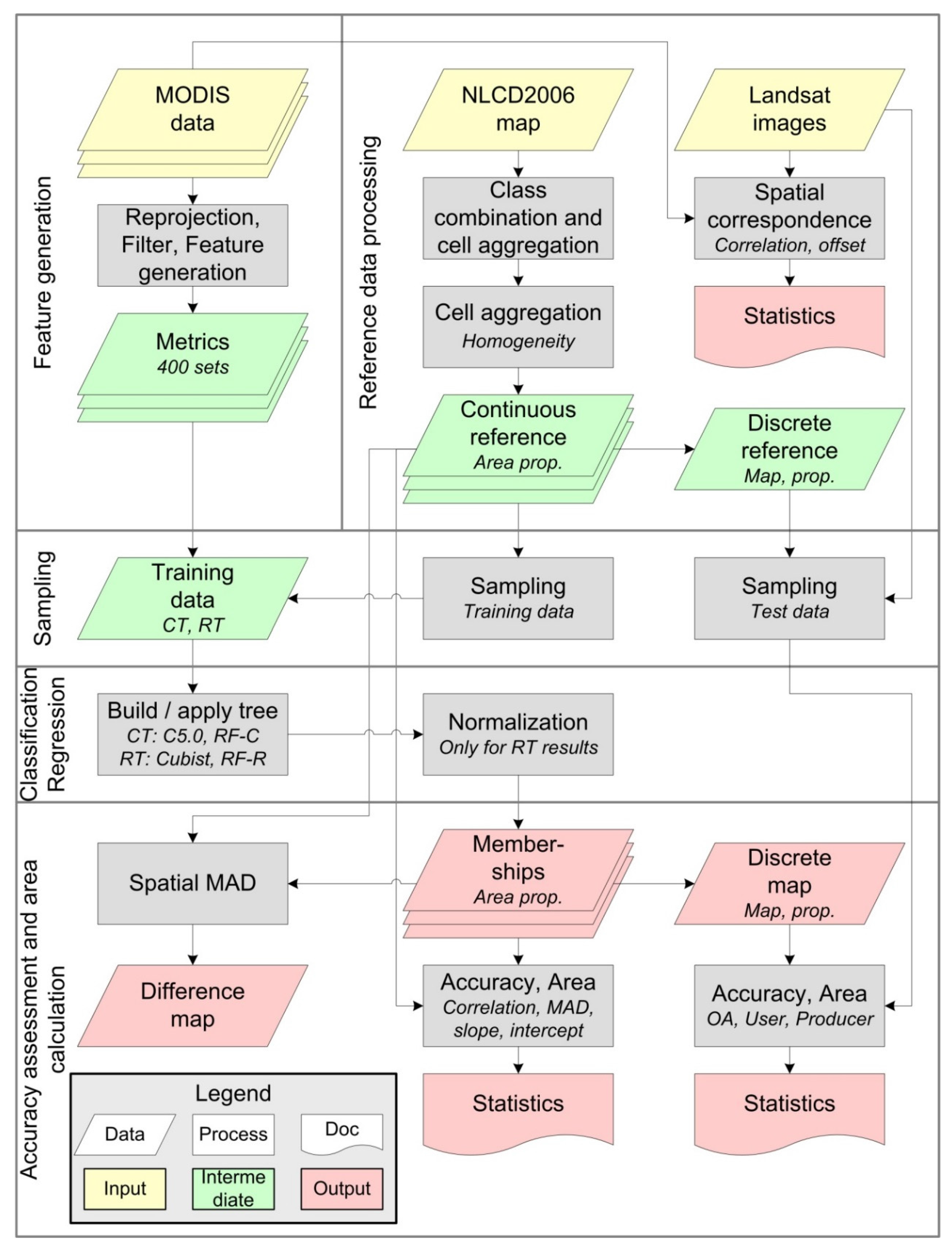
A common classification process similar to Blanco et al. [7], Clark et al. [21], and Colditz et al. [43] was used. Figure 2 illustrates this process which can be divided into five general blocks for (1) feature generation; (2) reference data processing; (3) training data sampling; (4) classification/regression; and (5) accuracy assessment and area calculation.

3.1. Feature Sets

The product quality for each pixel was analyzed using the Time Series Generator (TiSeG) [44]. Only best observations for each band with a generally good quality and no snow cover were selected, and data gaps were temporally interpolated with a linear function. Additionally, the NDVI was computed from red and near infrared bands.

The usefulness of metrics, which are univariate statistics computed over a defined period, for land cover mapping has been demonstrated in several other studies [7,21,33,43]. The mean, standard deviation, minimum and maximum value, and range between the minimum and maximum for the period of the entire year, two six-month, three four-month, and four three-month periods were computed from time series of each spectral band and the NDVI. This results in a feature set of 400 variables (seven spectral bands + NDVI, five univariate statistics, 10 periods).

Figure 2. Process-flow for data processing and map assessment. OA: overall accuracy, MAD: mean absolute difference, CT: classification tree, RT: regression tree, RF-C: Random Forest Classification, RF-R: Random Forest Regression, prop: proportion.

Figure 2. Process-flow for data processing and map assessment. OA: overall accuracy, MAD: mean absolute difference, CT: classification tree, RT: regression tree, RF-C: Random Forest Classification, RF-R: Random Forest Regression, prop: proportion.

3.2. Reference Data Processing

3.2.1. Spatial Co-Registration

A prerequisite of this study is near-to-perfect spatial co-registration between MODIS and Landsat images from which NLCD2006 was mapped. Spatial co-registration errors were estimated with an iterative two-step approach: (1) coarsening Landsat data to the MODIS grid cell size and (2) correlation. This process was repeated within a defined window displacing Landsat data by a specified interval in x- and y-direction, and the offset with the highest correlation coefficient indicates the displacement between both images [45]. In this study, the correlations are based on the NDVI from downloaded Landsat images and the closest available MODIS composite.

3.2.2. NLCD2006 Data

For this study 15 classes present in the subset of 30m NLCD2006 in the southeastern United States were combined to a final set of nine classes (Table 1). Next, blocks of 30 × 30 cells that spatially match one MODIS pixel were aggregated. Homogeneity H describes for each 900m MODIS pixel the area proportion of each land cover class from corresponding NLCD2006 data. In equation 1 x and y refer to individual pixels in NLCD2006, and expression c(x,y) = i counts all pixels in that block that correspond to class i. As a result, homogeneity, expressed in percentage, represents for each class the area proportion at the coarse grid.

$$H_i=\frac{{{\displaystyle \sum }}_{x=1}^{30}{{\displaystyle \sum }}_{y=1}^{30}c\left(x,y\right)=i}{30\times 30}\times 100$$

(1)

The argument maximum, argmax(H), also known as the majority rule, extracts the dominant class for each MODIS pixel. The corresponding area proportion, the homogeneity value of that dominant class, max(H), indicates the level of dominance in percent.

Table 1. Legend and area of each class from NLCD2006. Class 12: Perennial ice/snow was not present in the study area.

Class	Abbreviation	Area (Mio ha)	Area (%)	Classes in NLCD2006
Water	Wat	3.09	1.91	11: Open water
Developed	Dev	12.18	7.52	21–24: Developed, open space, low-high intensity; 31: Barren land
Deciduous forest	DF	38.63	23.84	41: Deciduous forest
Evergreen forest	EF	21.76	13.43	42: Evergreen forest; 43: Mixed forest
Shrubland	Shb	10.23	6.31	52: Shrub/scrub
Grassland	Grs	20.15	12.44	71: Grassland/herbaceous
Pasture	Past	22.18	13.69	81: Pasture/hay
Cultivated crops	Crop	24.87	15.35	82: Cultivated crops
Wetland	Wet	8.92	5.51	90: Woody wetlands; 95: Emergent herbaceous wetlands

Table 1. Legend and area of each class from NLCD2006. Class 12: Perennial ice/snow was not present in the study area.

Class	Abbreviation	Area (Mio ha)	Area (%)	Classes in NLCD2006
Water	Wat	3.09	1.91	11: Open water
Developed	Dev	12.18	7.52	21–24: Developed, open space, low-high intensity; 31: Barren land
Deciduous forest	DF	38.63	23.84	41: Deciduous forest
Evergreen forest	EF	21.76	13.43	42: Evergreen forest; 43: Mixed forest
Shrubland	Shb	10.23	6.31	52: Shrub/scrub
Grassland	Grs	20.15	12.44	71: Grassland/herbaceous
Pasture	Past	22.18	13.69	81: Pasture/hay
Cultivated crops	Crop	24.87	15.35	82: Cultivated crops
Wetland	Wet	8.92	5.51	90: Woody wetlands; 95: Emergent herbaceous wetlands

3.3. Training Data Sampling

3.3.1. Training of Classification Trees

A total of 5400 training samples (0.25% of the study area) were allocated from the homogeneity of NLCD2006 with a minimum distance of five pixels apart. For homogeneous training data the required number for each class was allocated with H = 100% which was decreased if this number could not be achieved [27]. Heterogeneous training data were allocated uniformly across six bins, with one bin for H = 100 and five bins for 100% > H ≥ 50% with 10% intervals. An alternative heterogeneous training set used random allocation.

With respect to between-class sample balance, this study compares (1) random sampling; (2) allocation proportional to the expected area as obtained from NLCD2006; and (3) equal number of samples for all classes. Since random and area-proportional allocation can lead to a very low number of samples for scarce classes, a minimum of 50 samples per class (1% of all samples) was required.

3.3.2. Training of Regression Trees

As for each class a separate regression tree has to be trained, the issue of between-class allocation becomes irrelevant. More important are allocation schemes across different levels of homogeneity, which was divided in 12 bins (H = 0%, ten bins with 0% < H < 100% with 10% intervals, and H = 100%). For each class, 5400 samples were allocated, testing three schemes: (1) random allocation with a minimum of 50 samples per bin (Random-50), (2) random allocation with no minimum per bin (Random-0), and (3) a uniform allocation with 450 samples per bin.

3.4. Classification and Regression Trees

3.4.1. Classification Trees

Classification trees (CT) apply recursive partitioning to a set of discrete (categorical) training data with the goal to reduce the impurity among classes by selecting an appropriate discriminating feature and threshold [46,47]. Commonly, classification trees generate discrete maps in which the class is defined by the highest proportion of samples in each terminal node. However, additional strategies such as randomization [48] or the use of class frequency at the leaf level together with boosting [27,42] can be used to derive class memberships and thus continuous classifications.

C5.0 decision trees (www.rulequest.com) [49] in the tree-mode together with 10-folded boosting were used as the simplistic model. For each tree the proportion of each class in every leaf was calculated and for each class the trees were combined to estimate class memberships [43].

Random Forest Classification (RF-C) [48] uses the classification and regression tree (CART) algorithm [46] as base classifier. The version provided for R [50] was employed with default options, i.e., for each tree a set of 63.2% of the samples is extracted, the number of features is limited to 20 (the floored square root of the total features), and trees are grown with the Gini index until each leaf is pure. Class memberships were derived by the combination of 1000 trees.

3.4.2. Regression Trees

In contrast to classification trees, regression trees apply recursive partitioning to a set of continuous training data. They largely follow the same logic but use the reduction in standard deviation as criteria for feature and threshold selection. Regression models were generated for membership estimation of each class. An equation of Xu et al. [24] normalizes the regression value RV for class i among all classes J. This linear scaling function (Equation (2)) ensures that the membership total for each pixel will be 100%. The majority rule was used for transformation of regression results to discrete maps.

$$M_i=\frac{R{V}_i}{{{\displaystyle \sum }}_{i=1}^{J}R{V}_i}$$

(2)

Cubist, a rule-based classifier (www.rulequest.com) [51,52], was employed as simplistic regression model. Initially, a regression tree similar to regression in CART is generated. Subsequently the tree is simplified and transformed into a set of rules with multiple conditions, and a multivariate regression equation estimates the numeric value. Thus, models from Cubist are not regression trees in a strict sense, however they yield promising results and were successfully employed in remote sensing [1,25,34,53,54]. The options for unbiased value estimation, no extrapolation of data values beyond training data range, and 5 committee models (similar to five-folded boosting) were selected.

Random Forest Regression (RF-R) uses the regression tree option of CART as base classifier [46]. Unlike Cubist, CART regression trees use the value estimate at the leaf level. The version provided for R [49] was executed with default options, i.e., for each tree a set of 63.2% of the samples is extracted, the number of features is 133 (total features/3, floored), and trees are grown with the standard deviation as splitting criterion, a minimum node size of 5 samples, and the numeric value is the mean of all samples in a leaf. The average of 1000 trees derived the class membership.

3.5. Accuracy Assessment and Area Estimation

3.5.1. Discrete Map Assessment

From a set of potential samples, constrained to the location of Landsat path rows (Figure 1) and having a homogeneity greater than 50% (H > 50%), 150 samples per strata, i.e., the class as defined in NLCD2006, were extracted. As response data served Landsat imagery from the year 2006 and very high resolution Google Earth data as close as possible to the year 2006. It is important to note that NLCD2006 only served for stratification to ensure that some samples will correspond to scarce and scattered classes, but it was not consulted by the analyst to assign the reference label. This approach also allowed for a better comparison among all classifications using the same reference set.

Due to ambiguity in interpretation of coarse cells, either uncertainty in the interpretation or presence of more than one land cover type in a coarse resolution cell of 900 m (mixed pixel issue), it is recommended to assign two labels [7,23]. The primary class is the most likely call, i.e., the most certain class or class with the largest area proportion, and the alternative label indicates the potential of presence of another class. In case of high certainty or presence of only one class both labels are the same.

Discrete maps were assessed with (1) only using the primary reference label or (2) the primary + alternative reference label. In the latter case, the land cover map was considered as correctly classified if it corresponded to the primary or the alternative reference label; in case of disagreement with both the primary class was used to assign the error in the confusion matrix. The overall accuracy (OA, sum of the diagonal against the total of the error matrix) as well as users and producers accuracies were employed using standard formulas for confidence estimation [55].

Pair-wise comparisons of accuracies were performed in two ways. The McNemar test aims at the difference between correctly and incorrectly classified class allocations [56]. This test is recommended as the reference set was identical for the assessment of all maps [57], and the z-test form (Equation (3)) was implemented where f_AB and f_BA indicate the frequency of correctly classified in map A but incorrectly in map B and vice versa.

$$z=\frac{\left|f_{AB}-f_{BA}\right|}{\sqrt{f_{AB}+f_{BA}}}$$

(3)

The overall accuracy was tested with standard z-test-statistic (Equation (4)) where OA_A and OA_B are the overall accuracies of map A and map B and SD_A and SD_B are their respective standard deviations.

$$z=\frac{\left|O{A}_A-O{A}_B\right|}{\sqrt{S{D_A}^2+S{D_B}^2}}$$

(4)

3.5.2. Continuous Map Assessment

Class memberships were assessed with four measures against the homogeneity from NLCD2006 as continuous reference set. The coefficient of correlation r is a means to evaluate the strength of agreement between the membership and reference set. The mean absolute difference (MAD, Equation (5)) addresses the absolute error in percent between the membership estimates (M) and reference set (R) for all pixels (K). For a spatial representation of the error, MAD was computed for each pixel with K being the total of classes for one pixel. The slope and intercept of the linear regression function between reference and membership indicate the dynamic range of the predicted values and the bias.

$$MAD=\frac{{{\displaystyle \sum }}_{k=1}^K\left|M_k-R_k\right|}{K}$$

(5)

3.5.3. Area Estimation

Area estimation from discrete maps is a straight-forward pixel count for class i multiplied by the area of each pixel. The area of each class from memberships is the total of all membership values times their pixel area [15]. The total absolute difference in area (AD) between reference R (NLCD2006) and classification or membership CM, with K being the total of all pixels, was calculated using Equation (6) and expressed in area and in percent against the total of the study area.

$$AD={\displaystyle \sum }_{k=1}^K\left|R_k-C{M}_k\right|$$

(6)

4. Results and Analysis

4.1. Reference Data

4.1.1. Spatial Co-Registration

Table 2 shows near-to-perfect spatial co-registration between NDVI from ten Landsat images and corresponding dates of MODIS composites. The offsets are negligible, with averages of x = −3 m, y = −3 m and extremes lower-equal ±30 m. The coefficient values itself are all positive and indicate a sufficiently high correlation, i.e., the spatial patterns in Landsat and MODIS NDVI are closely related to each other. This finding is an important prerequisite for the following analysis as it permits a direct relation between Landsat-based NLCD2006 maps and MODIS.

Table 2. Spatial offset between Landsat images (for their spatial location see Figure 1) and temporally corresponding composites of MODIS data using the NDVI.

Path-Row	Location	Acquisition of Landsat Image	X-Offset (m)	Y-offset (m)	Correlation Coefficient
021-037	East Gulf Coastal Plain, AL	15 June 2006	−30	30	0.71
025-036	Ouachita Mountains, AR	15 September 2006	−30	0	0.76
018-038	East Gulf Coastal Plain, GA	10 June 2006	0	0	0.74
028-034	Osage Plains, KS	13 April 2006	−30	−30	0.83
020-034	Interior Low Plateaus, KY	23 May 2006	30	−30	0.75
023-037	Mississippi Valley MS	3 October 2006	−30	0	0.90
023-034	Mississippi Valley, MO	31 July 2006	30	−30	0.55
018-036	Piedmont, SC	10 June 2006	0	0	0.68
027-037	Dallas Area, TX	13 September 2006	0	30	0.86
028-038	Central Texas, TX	20 September 2006	30	0	0.84

Table 2. Spatial offset between Landsat images (for their spatial location see Figure 1) and temporally corresponding composites of MODIS data using the NDVI.

Path-Row	Location	Acquisition of Landsat Image	X-Offset (m)	Y-offset (m)	Correlation Coefficient
021-037	East Gulf Coastal Plain, AL	15 June 2006	−30	30	0.71
025-036	Ouachita Mountains, AR	15 September 2006	−30	0	0.76
018-038	East Gulf Coastal Plain, GA	10 June 2006	0	0	0.74
028-034	Osage Plains, KS	13 April 2006	−30	−30	0.83
020-034	Interior Low Plateaus, KY	23 May 2006	30	−30	0.75
023-037	Mississippi Valley MS	3 October 2006	−30	0	0.90
023-034	Mississippi Valley, MO	31 July 2006	30	−30	0.55
018-036	Piedmont, SC	10 June 2006	0	0	0.68
027-037	Dallas Area, TX	13 September 2006	0	30	0.86
028-038	Central Texas, TX	20 September 2006	30	0	0.84

4.1.2. NLCD2006 Data

Figure 3A shows the NLCD2006 map recoded to nine classes (Table 1) at 30 m spatial resolution. The map illustrates some spatial details such as the road network in Kansas that disappeared in Figure 3B, showing the spatial distribution of the dominant class at 900 m spatial resolution derived with majority rule argmax(H). Figure 3C indicates the corresponding area proportion of the dominating class, max(H). There are distinct regional patterns with homogeneous areas in the western portion (Shrubland, Grassland, Cultivated crops), the Mississippi valley (Cultivated crops), the southern Ozark and Appalachians mountains (Deciduous forest), the Okefenokee Swamp in southern Georgia (Wetlands), and large metropolitan areas like Atlanta, Dallas-Fort Worth, and St. Louis (Developed). In particular, the southeastern region is highly heterogeneous with area proportions of the dominating class below 50%; similar heterogeneous patterns exist in eastern Texas, Oklahoma, Louisiana, and Arkansas.

Figure 3. (A) Reference map at 30m spatial resolution; (B) coarsened map at 900 m using majority rule, argmax(H); and (C) area proportion of that class, max(H).

Figure 3. (A) Reference map at 30m spatial resolution; (B) coarsened map at 900 m using majority rule, argmax(H); and (C) area proportion of that class, max(H).

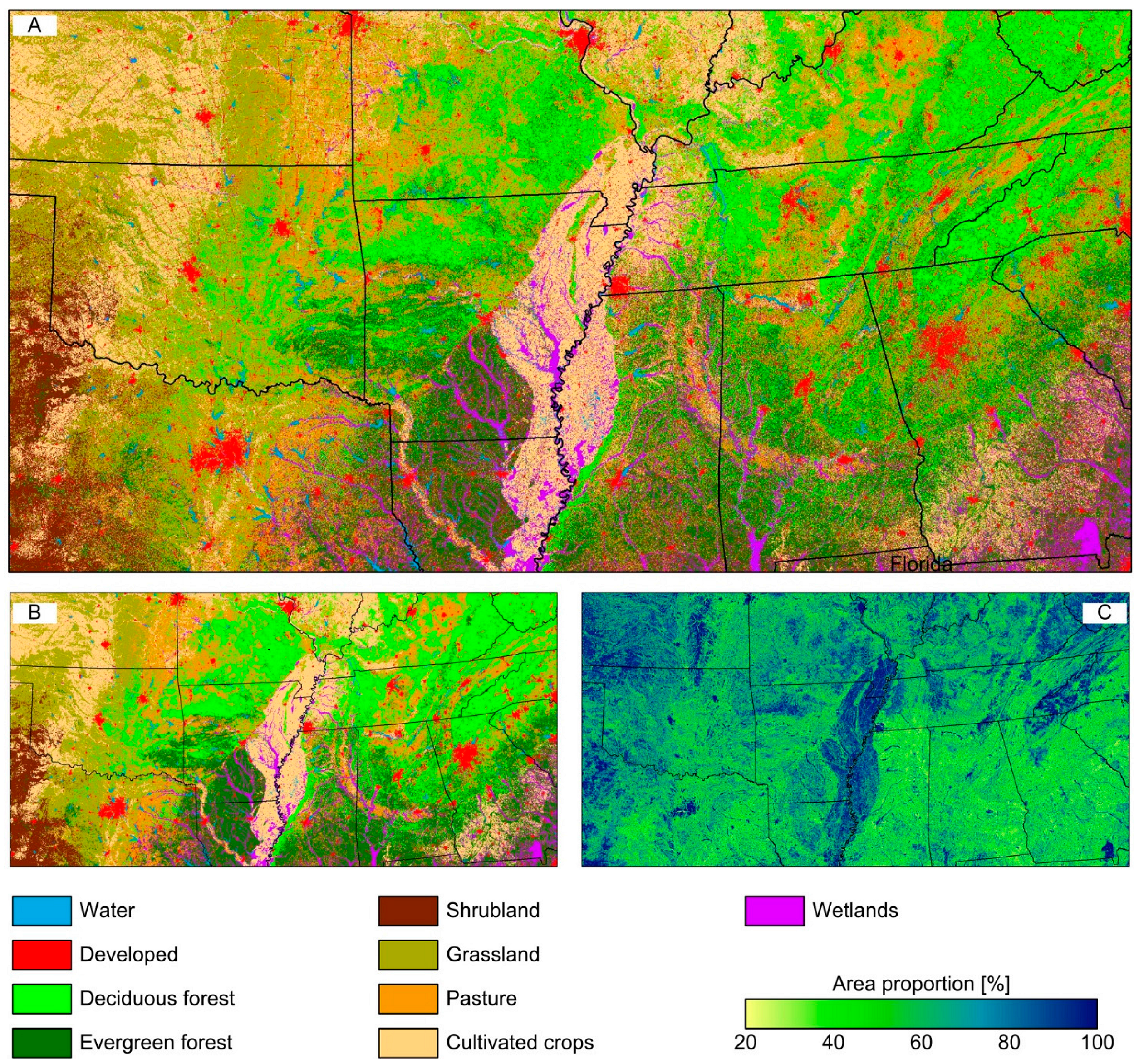
Table 3 shows for each class the percentage of homogeneity in 12 bins. It is evident that there are more pixels with low homogeneity, but the magnitude is different for each class. For instance, class Water only exists in selected parts of the map and thus H = 0% makes up 76.7% of the study area. Class Deciduous forest is rather ubiquitous with a proportion of 37.6% for 10% ≤ H < 60%. Due to many roads that cause a homogeneity slightly above 0%, class Developed is an interesting example with only 21.3% for H = 0% but 61.5% for 0% < H < 10%.

Table 3. Homogeneity (H) in 10-percent bins and bins for 0 and 100 percent derived from NLCD2006. For abbreviations of class names see Table 1.

Homogeneity (%)	Wat	Dev	DF	EF	Shb	Grs	Past	Crop	Wet
H = 0	76.67	21.32	23.43	39.92	55.22	39.46	47.16	58.16	61.32
0 < H < 10	19.39	61.45	24.37	26.40	27.14	33.34	18.13	12.89	24.46
10 ≤ H < 20	1.53	10.36	12.01	9.50	8.10	8.10	9.33	5.52	5.63
20 ≤ H < 30	0.65	2.28	8.73	6.45	3.72	4.31	6.60	3.75	2.90
30 ≤ H < 40	0.38	1.08	6.86	4.87	1.77	3.08	5.20	3.02	1.69
40 ≤ H < 50	0.29	0.74	5.51	3.84	1.02	2.48	4.21	2.63	1.09
50 ≤ H < 60	0.23	0.57	4.52	3.05	0.73	2.09	3.34	2.41	0.76
60 ≤ H < 70	0.18	0.48	3.86	2.40	0.59	1.81	2.59	2.34	0.56
70 ≤ H < 80	0.17	0.45	3.52	1.79	0.52	1.62	1.88	2.45	0.45
80 ≤ H < 90	0.15	0.42	3.39	1.23	0.49	1.53	1.16	2.89	0.41
90 ≤ H < 100	0.19	0.49	3.37	0.56	0.59	1.91	0.40	3.60	0.52
H = 100	0.18	0.36	0.41	0.01	0.12	0.26	0.01	0.35	0.22

Table 3. Homogeneity (H) in 10-percent bins and bins for 0 and 100 percent derived from NLCD2006. For abbreviations of class names see Table 1.

Homogeneity (%)	Wat	Dev	DF	EF	Shb	Grs	Past	Crop	Wet
H = 0	76.67	21.32	23.43	39.92	55.22	39.46	47.16	58.16	61.32
0 < H < 10	19.39	61.45	24.37	26.40	27.14	33.34	18.13	12.89	24.46
10 ≤ H < 20	1.53	10.36	12.01	9.50	8.10	8.10	9.33	5.52	5.63
20 ≤ H < 30	0.65	2.28	8.73	6.45	3.72	4.31	6.60	3.75	2.90
30 ≤ H < 40	0.38	1.08	6.86	4.87	1.77	3.08	5.20	3.02	1.69
40 ≤ H < 50	0.29	0.74	5.51	3.84	1.02	2.48	4.21	2.63	1.09
50 ≤ H < 60	0.23	0.57	4.52	3.05	0.73	2.09	3.34	2.41	0.76
60 ≤ H < 70	0.18	0.48	3.86	2.40	0.59	1.81	2.59	2.34	0.56
70 ≤ H < 80	0.17	0.45	3.52	1.79	0.52	1.62	1.88	2.45	0.45
80 ≤ H < 90	0.15	0.42	3.39	1.23	0.49	1.53	1.16	2.89	0.41
90 ≤ H < 100	0.19	0.49	3.37	0.56	0.59	1.91	0.40	3.60	0.52
H = 100	0.18	0.36	0.41	0.01	0.12	0.26	0.01	0.35	0.22

4.2. Sample Allocation of Training Data

This section exemplarily demonstrates training sample allocation schemes. Each of the following tables shows the expected sample frequency, which is calculated from the number of samples that fulfill the specific allocation criteria, the corresponding expected number of samples, in many cases considering a minimum of 50 samples per class or sample bin, followed by actual sample allocation. All numbers are specific for this study and are meant to demonstrate the sample allocation process in practice.

Table 4 presents the random sample allocation for homogeneous pixels. The expected frequency and thus the expected number of samples is relative to the class proportion of H = 100% in Table 3. Actual sampling starts at H = 100% and decreases until the expected number of samples per class is reached. Sufficient samples of fully homogeneous pixels (H = 100%) were available for classes Deciduous forest, Grassland, and Cultivated crops. To reach the expected number of 358 samples for class Shrubland, Homogeneity had to be decreased to 96%.

Table 4. Random allocation with a minimum of 50 samples per class using homogeneous pixels H = 100%. Homogeneity (H) in percent. See Table 1 for abbreviations of class names.

	Wat	Dev	DF	EF	Shb	Grs	Past	Crop	Wet
Expected sample frequency (%)	9.29	18.70	21.46	0.44	6.23	13.77	0.31	18.26	11.54
Expected number of samples	510	976	1112	72	358	731	66	954	621
H = 100%	352	623	1112	28	181	731	0	954	420
99% ≤ H < 100%	71	172	0	44	71	0	66	0	170
98% ≤ H < 99%	53	117	0	0	56	0	0	0	31
97% ≤ H < 98%	34	64	0	0	47	0	0	0	0
96% ≤ H < 97%	0	0	0	0	3	0	0	0	0

Table 4. Random allocation with a minimum of 50 samples per class using homogeneous pixels H = 100%. Homogeneity (H) in percent. See Table 1 for abbreviations of class names.

	Wat	Dev	DF	EF	Shb	Grs	Past	Crop	Wet
Expected sample frequency (%)	9.29	18.70	21.46	0.44	6.23	13.77	0.31	18.26	11.54
Expected number of samples	510	976	1112	72	358	731	66	954	621
H = 100%	352	623	1112	28	181	731	0	954	420
99% ≤ H < 100%	71	172	0	44	71	0	66	0	170
98% ≤ H < 99%	53	117	0	0	56	0	0	0	31
97% ≤ H < 98%	34	64	0	0	47	0	0	0	0
96% ≤ H < 97%	0	0	0	0	3	0	0	0	0

Table 5 shows the allocation proportional to the expected area from NLCD2006 (Table 1). Heterogeneous pixels were allocated uniformly across six bins of H ≥ 50%. Sampling should start at the bin with the highest homogeneity (H = 100%) because in some cases the expected sample size may not be available and will be allocated from the next bin. For instance, for class Evergreen forest with an expected total of 715 samples each bin should contain 119.17 samples (rounded to 119 or 120 samples), but only 29 samples could be selected for H = 100% and the remaining 90 samples were allocated from bin 90% ≤ H < 100%.

Table 5. Allocation proportional to expected area with a minimum of 50 samples per class using heterogeneous pixels with uniform allocation across six bins of H ≥ 50%. Homogeneity (H) in percent. For abbreviations of class names see Table 1.

	Wat	Dev	DF	EF	Shb	Grs	Past	Crop	Wet
Expected sample frequency (%)	1.91	7.52	23.84	13.43	6.31	12.44	13.69	15.35	5.51
Expected number of samples	145	422	1230	715	362	666	727	810	323
H = 100%	24	70	205	29	60	111	0	135	54
90% ≤ H < 100%	24	71	205	209	61	111	242	135	54
80% ≤ H < 90%	25	70	205	120	60	111	122	135	54
70% ≤ H < 80%	24	70	205	119	60	111	121	135	53
60% ≤ H < 70%	24	71	205	119	61	111	121	135	54
50% ≤ H < 60%	24	70	205	119	60	111	121	135	54

Table 5. Allocation proportional to expected area with a minimum of 50 samples per class using heterogeneous pixels with uniform allocation across six bins of H ≥ 50%. Homogeneity (H) in percent. For abbreviations of class names see Table 1.

	Wat	Dev	DF	EF	Shb	Grs	Past	Crop	Wet
Expected sample frequency (%)	1.91	7.52	23.84	13.43	6.31	12.44	13.69	15.35	5.51
Expected number of samples	145	422	1230	715	362	666	727	810	323
H = 100%	24	70	205	29	60	111	0	135	54
90% ≤ H < 100%	24	71	205	209	61	111	242	135	54
80% ≤ H < 90%	25	70	205	120	60	111	122	135	54
70% ≤ H < 80%	24	70	205	119	60	111	121	135	53
60% ≤ H < 70%	24	71	205	119	61	111	121	135	54
50% ≤ H < 60%	24	70	205	119	60	111	121	135	54

Table 6 presents equal allocation between classes of heterogeneous pixels with random allocation across sample bins of argmax(H). Although the lowest potential level of dominance could be as low as 11.1% (1/9 classes) in reality, the lowest homogeneity was above 20%. For most classes pixels are highly heterogeneous with 40% ≤ H < 70%, i.e., the area of the dominating class makes up approximately half of the pixel. Only classes Grassland and Cropland indicated more homogeneous pixels with 70% ≤ H < 100%.

Table 6. Equal class allocation of heterogeneous pixels with random allocation across bins of argmax(H). Homogeneity (H) in percent. See Table 1 for abbreviations of class names.

	Wat	Dev	DF	EF	Shb	Grs	Past	Crop	Wet
Expected sample frequency (%)	11.11	11.11	11.11	11.11	11.11	11.11	11.11	11.11	11.11
Expected number of samples	600	600	600	600	600	600	600	600	600
H = 100%	42	36	6	0	9	14	0	14	20
90% ≤ H < 100%	54	66	62	20	50	100	12	121	60
80% ≤ H < 90%	62	59	82	38	55	100	48	94	61
70% ≤ H < 80%	63	71	82	73	66	92	93	101	46
60% ≤ H < 70%	68	84	94	102	95	83	97	87	69
50% ≤ H < 60%	108	90	104	131	117	91	137	73	104
40% ≤ H < 50%	108	96	101	120	103	73	132	71	109
30% ≤ H < 40%	80	75	58	94	75	40	69	27	101
20% ≤ H < 30%	15	23	11	22	30	7	12	12	30

Table 6. Equal class allocation of heterogeneous pixels with random allocation across bins of argmax(H). Homogeneity (H) in percent. See Table 1 for abbreviations of class names.

	Wat	Dev	DF	EF	Shb	Grs	Past	Crop	Wet
Expected sample frequency (%)	11.11	11.11	11.11	11.11	11.11	11.11	11.11	11.11	11.11
Expected number of samples	600	600	600	600	600	600	600	600	600
H = 100%	42	36	6	0	9	14	0	14	20
90% ≤ H < 100%	54	66	62	20	50	100	12	121	60
80% ≤ H < 90%	62	59	82	38	55	100	48	94	61
70% ≤ H < 80%	63	71	82	73	66	92	93	101	46
60% ≤ H < 70%	68	84	94	102	95	83	97	87	69
50% ≤ H < 60%	108	90	104	131	117	91	137	73	104
40% ≤ H < 50%	108	96	101	120	103	73	132	71	109
30% ≤ H < 40%	80	75	58	94	75	40	69	27	101
20% ≤ H < 30%	15	23	11	22	30	7	12	12	30

Table 7 shows sample allocation schemes for regression trees for class Evergreen forest. Heterogeneous pixels were allocated randomly or uniformly across all bins of homogeneity (see also Table 3). In case of insufficient available samples for a bin starting at H = 100%, the remaining samples were added to the next bin.

Table 7. Random and uniform allocation of heterogeneous pixels for regression trees for class Evergreen forest. Homogeneity (H) in percent.

	Random-50			Random-0			Uniform
	Expected Sample Frequency (%)	Expected Number of Samples	Actual Number of Samples	Expected Sample Frequency (%)	Expected Number of Samples	Actual Number of Samples	Expected Sample Frequency (%)	Expected Number of Samples	Actual Number of Samples
H = 100	0.01	50	29	0.01	0	0	8.33	450	29
90 ≤ H < 100	0.56	77	98	0.56	31	31	8.33	450	871
80 ≤ H < 90	1.23	109	109	1.23	66	66	8.33	450	450
70 ≤ H < 80	1.79	136	136	1.79	97	97	8.33	450	450
60 ≤ H < 70	2.40	165	165	2.40	129	129	8.33	450	450
50 ≤ H < 60	3.05	197	197	3.05	165	165	8.33	450	450
40 ≤ H < 50	3.84	234	234	3.84	207	207	8.33	450	450
30 ≤ H < 40	4.87	283	283	4.87	263	263	8.33	450	450
20 ≤ H < 30	6.45	360	360	6.45	348	348	8.33	450	450
10 ≤ H < 20	9.50	505	505	9.50	513	513	8.33	450	450
0 < H < 10	26.40	1318	1318	26.40	1425	1425	8.33	450	450
H = 0	39.92	1966	1966	39.92	2156	2156	8.33	450	450

Table 7. Random and uniform allocation of heterogeneous pixels for regression trees for class Evergreen forest. Homogeneity (H) in percent.

	Random-50			Random-0			Uniform
	Expected Sample Frequency (%)	Expected Number of Samples	Actual Number of Samples	Expected Sample Frequency (%)	Expected Number of Samples	Actual Number of Samples	Expected Sample Frequency (%)	Expected Number of Samples	Actual Number of Samples
H = 100	0.01	50	29	0.01	0	0	8.33	450	29
90 ≤ H < 100	0.56	77	98	0.56	31	31	8.33	450	871
80 ≤ H < 90	1.23	109	109	1.23	66	66	8.33	450	450
70 ≤ H < 80	1.79	136	136	1.79	97	97	8.33	450	450
60 ≤ H < 70	2.40	165	165	2.40	129	129	8.33	450	450
50 ≤ H < 60	3.05	197	197	3.05	165	165	8.33	450	450
40 ≤ H < 50	3.84	234	234	3.84	207	207	8.33	450	450
30 ≤ H < 40	4.87	283	283	4.87	263	263	8.33	450	450
20 ≤ H < 30	6.45	360	360	6.45	348	348	8.33	450	450
10 ≤ H < 20	9.50	505	505	9.50	513	513	8.33	450	450
0 < H < 10	26.40	1318	1318	26.40	1425	1425	8.33	450	450
H = 0	39.92	1966	1966	39.92	2156	2156	8.33	450	450

4.3. Accuracy Assessment of Classification and Regression Trees

4.3.1. Reference Data for Discrete Map Assessment

Table 8 provides details on the reference sample allocation process and reference label assignment. For each class, the number of potential samples (each sample corresponds to one 900 m MODIS pixel) meets the following conditions: (1) its homogeneity in NLCD2006 is higher than 50% and (2) it is located within the extent of Landsat images (Figure 1). The average of the homogeneity shows that, albeit all samples belong in majority to one class (H > 50%), the level of dominance is moderate and most samples are not pure. For each stratum in NLCD2006, 150 samples were extracted. Out of 1350 samples, four were excluded from analysis because response data were obscured by clouds or class assignment was too uncertain. The columns for primary and alternative label indicate for each class the number of assigned reference samples. For instance, there are 120 samples with primary label of class Water and another 84 samples labeled as Water by the alternative call. For 73 samples, the primary and alternative calls agree, i.e., class assignment is quite certain. On the other hand, there are 47 samples for which the alternative class was not Water and 11 samples for which the primary call was not Water. As the assignment of Water in image interpretation is quite simple, these samples were likely located along the edge of a water body and contain a mixture of land cover types. There are extreme cases of ambiguity such as Grassland and Pasture, both indicating a specific land use difficult to classify only using satellite imagery, or frequently mixed pixels, e.g., Wetland. Less than half of the samples (48.8%) had corresponding class labels in the primary and alternative call.

Table 8. Sample allocation from NLCD2006 (H > 50%) and location in Landsat path-rows (Figure 1) and primary and alternative reference label assignment from Landsat and Google Earth image interpretation. Agreement shows the number of samples with equal primary and alternative label. Homogeneity (H) in percent.

Class/Strata	NLCD-Based Sample Allocation		Reference Set from Response data
	Potential Samples	Mean (H)	Primary	Alternative	Agreement
Water	4857	76.67	120	84	73
Developed	14,197	79.32	155	153	130
Deciduous forest	60,678	72.35	322	309	193
Evergreen forest	35,733	67.06	90	84	20
Shrubland	17,996	71.40	178	196	111
Grassland	36,388	73.58	96	155	6
Pasture	32,439	66.88	121	123	1
Cropland	63,522	77.81	218	171	108
Wetland	11,502	74.47	46	71	15

Table 8. Sample allocation from NLCD2006 (H > 50%) and location in Landsat path-rows (Figure 1) and primary and alternative reference label assignment from Landsat and Google Earth image interpretation. Agreement shows the number of samples with equal primary and alternative label. Homogeneity (H) in percent.

Class/Strata	NLCD-Based Sample Allocation		Reference Set from Response data
	Potential Samples	Mean (H)	Primary	Alternative	Agreement
Water	4857	76.67	120	84	73
Developed	14,197	79.32	155	153	130
Deciduous forest	60,678	72.35	322	309	193
Evergreen forest	35,733	67.06	90	84	20
Shrubland	17,996	71.40	178	196	111
Grassland	36,388	73.58	96	155	6
Pasture	32,439	66.88	121	123	1
Cropland	63,522	77.81	218	171	108
Wetland	11,502	74.47	46	71	15

4.3.2. Discrete Map Assessment

The overall accuracies (OA) of all classifications for discrete maps are shown in Table 9 for the primary reference label (P) or the primary and alternative label (P + A) as correctly classified. Confidence intervals (p < 5%, two tailed z-test) range between 2.5% and 2.7% and are therefore not presented.

Overall accuracies of RF-C are, on average, 1% higher than from C5.0, and Cubist yields about 0.5% higher accuracies than RF-R. Assessing discrete maps from classification trees (C5.0, RF-C), heterogeneous training pixels show, on average, 6% better accuracy than homogeneous training data. There are no notable differences between uniform or random allocation of heterogeneous training samples. Area-proportional between-class sample allocations show 1% higher overall accuracies than equalized sampling, and accuracy for random training sampling decreases another 0.5%. Discrete maps from regression trees show a consistent pattern of 2%–3% higher accuracies for uniform allocation. Random allocation with no minimum sample size per bin resulted in 1%–2% lower accuracies than when allocating at least 50 samples for each bin. Note that normalization has no effect on discrete maps obtained with the majority rule. Best results for classification trees were obtained with RF-C, uniform allocation and area-balanced between-class sample allocation and for regression trees with uniform sampling but negligible differences between Cubist and RF-R (highlighted cells in Table 9).

Assessments using the primary and alternative reference label as correctly classified result in, on average, 14% higher accuracies, which indicates ambiguity in reference label assignment of some classes. In terms of class accuracies (see supplemental material), Water and Developed are well classified (on average 75% or better in users and producers accuracy). Shrubland and Cropland form a second group with above 50% in both class accuracies. There is confusion between Evergreen and Deciduous forest, and between both classes and Wetland as many forests in the southeastern US are interconnected with wetlands either as riparian vegetation or along estuaries at the coast. It should be considered that Wetland was the class with lowest accuracies in NLCD [40]. Other classes with below 50% class accuracy are Pasture and Grassland as both indicate land use forms of herbaceous areas.

Table 9. Accuracy measures and absolute difference in area for discrete and continuous (class memberships) classifications. OA: overall accuracy using primary (P) or primary and alternative (P + A) label of reference data as correctly classified. r: correlation coefficient. MAD: mean absolute difference. Int: Intercept. AD: absolute difference in million hectares and percent. Classification trees C5.0 and Random forest classification (RF-C) with homogeneous samples (H = 100) or heterogeneous samples allocated uniformly for H ≥ 50% or randomly (argmax(H)). Sample allocation between classes with random, area-proportional, equal allocation. Regression trees Cubist and Random Forest Regression (RF-R) with uniform and random allocation with no minimum or at least 50 samples per bin. NN: no normalization. Norm: normalization. Highlighted cells indicate best results for classification and regression trees.

Classification			Accuracy Discrete		Accuracy Continuous				AD Discrete		AD Continuous
Algorithm	Allocation	Class/Norm.	OA (%) P	OA (%) P + A	r	MAD (%)	Slope	Int. (%)	Mio ha	%	Mio ha	%
C5.0	Homogen	Random	46.14	56.24	0.64	9.94	0.70	3.32	89.99	55.55	85.47	52.76
		Area	49.63	62.11	0.74	8.75	0.85	1.65	48.77	30.10	47.90	29.57
		Equal	49.70	61.29	0.69	9.45	0.77	2.59	66.93	41.31	65.76	40.59
	Uniform	Random	52.23	65.23	0.81	7.34	0.90	1.12	28.73	17.73	15.45	9.54
		Area	54.53	67.83	0.81	7.25	0.89	1.20	23.35	14.41	8.52	5.26
		Equal	54.09	67.01	0.78	7.81	0.82	1.95	20.40	12.59	27.29	16.85
	Random	Random	53.12	67.38	0.81	7.16	0.85	1.68	32.41	20.01	15.26	9.42
		Area	53.79	66.86	0.81	7.22	0.82	2.00	21.78	13.44	7.11	4.39
		Equal	52.82	66.86	0.78	7.76	0.77	2.58	22.01	13.59	30.94	19.10
RF-C	Homogen	Random	47.03	57.06	0.67	9.49	0.71	3.19	91.14	56.26	82.34	50.83
		Area	49.78	63.22	0.76	8.31	0.87	1.45	46.06	28.43	45.81	28.28
		Equal	51.63	64.04	0.72	8.92	0.79	2.33	61.36	37.88	60.53	37.37
	Uniform	Random	53.27	67.24	0.83	7.02	0.92	0.82	31.89	19.68	16.83	10.39
		Area	55.57	69.47	0.83	6.96	0.91	0.96	22.82	14.09	8.74	5.39
		Equal	54.09	67.61	0.80	7.41	0.85	1.69	20.93	12.92	27.03	16.68
	Random	Random	52.97	67.24	0.83	6.70	0.87	1.39	36.55	22.56	18.03	11.13
		Area	54.75	68.72	0.83	6.67	0.85	1.66	27.37	16.90	6.36	3.93
		Equal	53.64	67.53	0.81	7.20	0.80	2.25	23.26	14.36	29.37	18.13
Cubist	Random-50	NN	53.79	68.50	0.86	6.25	0.85	2.79	29.14	17.99	16.20	10.00
		Norm	53.79	68.50	0.86	6.07	0.73	2.93	29.14	17.99	5.45	3.36
	Random-0	NN	51.93	65.90	0.86	5.95	0.76	2.56	35.36	21.83	2.51	1.55
		Norm	51.93	65.90	0.86	5.93	0.75	2.71	35.36	21.83	4.22	2.61
	Uniform	NN	55.94	69.84	0.79	12.37	0.86	11.71	15.32	9.46	148.94	91.94
		Norm	55.94	69.84	0.81	8.79	0.46	5.96	15.32	9.46	49.87	30.78
RF-R	Random-50	NN	53.19	66.79	0.85	6.95	0.81	4.11	31.02	19.15	29.84	18.42
		Norm	53.19	66.79	0.85	6.66	0.66	3.79	31.02	19.15	10.45	6.45
	Random-0	NN	51.41	65.75	0.86	6.54	0.73	3.59	39.21	24.20	9.15	5.65
		Norm	51.41	65.75	0.85	6.49	0.68	3.56	39.21	24.20	2.66	1.64
	Uniform	NN	56.24	69.76	0.77	14.24	0.81	14.26	16.20	10.00	177.88	109.80
		Norm	56.24	69.76	0.79	9.55	0.40	6.65	16.20	10.00	56.28	34.74

Table 9. Accuracy measures and absolute difference in area for discrete and continuous (class memberships) classifications. OA: overall accuracy using primary (P) or primary and alternative (P + A) label of reference data as correctly classified. r: correlation coefficient. MAD: mean absolute difference. Int: Intercept. AD: absolute difference in million hectares and percent. Classification trees C5.0 and Random forest classification (RF-C) with homogeneous samples (H = 100) or heterogeneous samples allocated uniformly for H ≥ 50% or randomly (argmax(H)). Sample allocation between classes with random, area-proportional, equal allocation. Regression trees Cubist and Random Forest Regression (RF-R) with uniform and random allocation with no minimum or at least 50 samples per bin. NN: no normalization. Norm: normalization. Highlighted cells indicate best results for classification and regression trees.

Classification			Accuracy Discrete		Accuracy Continuous				AD Discrete		AD Continuous
Algorithm	Allocation	Class/Norm.	OA (%) P	OA (%) P + A	r	MAD (%)	Slope	Int. (%)	Mio ha	%	Mio ha	%
C5.0	Homogen	Random	46.14	56.24	0.64	9.94	0.70	3.32	89.99	55.55	85.47	52.76
		Area	49.63	62.11	0.74	8.75	0.85	1.65	48.77	30.10	47.90	29.57
		Equal	49.70	61.29	0.69	9.45	0.77	2.59	66.93	41.31	65.76	40.59
	Uniform	Random	52.23	65.23	0.81	7.34	0.90	1.12	28.73	17.73	15.45	9.54
		Area	54.53	67.83	0.81	7.25	0.89	1.20	23.35	14.41	8.52	5.26
		Equal	54.09	67.01	0.78	7.81	0.82	1.95	20.40	12.59	27.29	16.85
	Random	Random	53.12	67.38	0.81	7.16	0.85	1.68	32.41	20.01	15.26	9.42
		Area	53.79	66.86	0.81	7.22	0.82	2.00	21.78	13.44	7.11	4.39
		Equal	52.82	66.86	0.78	7.76	0.77	2.58	22.01	13.59	30.94	19.10
RF-C	Homogen	Random	47.03	57.06	0.67	9.49	0.71	3.19	91.14	56.26	82.34	50.83
		Area	49.78	63.22	0.76	8.31	0.87	1.45	46.06	28.43	45.81	28.28
		Equal	51.63	64.04	0.72	8.92	0.79	2.33	61.36	37.88	60.53	37.37
	Uniform	Random	53.27	67.24	0.83	7.02	0.92	0.82	31.89	19.68	16.83	10.39
		Area	55.57	69.47	0.83	6.96	0.91	0.96	22.82	14.09	8.74	5.39
		Equal	54.09	67.61	0.80	7.41	0.85	1.69	20.93	12.92	27.03	16.68
	Random	Random	52.97	67.24	0.83	6.70	0.87	1.39	36.55	22.56	18.03	11.13
		Area	54.75	68.72	0.83	6.67	0.85	1.66	27.37	16.90	6.36	3.93
		Equal	53.64	67.53	0.81	7.20	0.80	2.25	23.26	14.36	29.37	18.13
Cubist	Random-50	NN	53.79	68.50	0.86	6.25	0.85	2.79	29.14	17.99	16.20	10.00
		Norm	53.79	68.50	0.86	6.07	0.73	2.93	29.14	17.99	5.45	3.36
	Random-0	NN	51.93	65.90	0.86	5.95	0.76	2.56	35.36	21.83	2.51	1.55
		Norm	51.93	65.90	0.86	5.93	0.75	2.71	35.36	21.83	4.22	2.61
	Uniform	NN	55.94	69.84	0.79	12.37	0.86	11.71	15.32	9.46	148.94	91.94
		Norm	55.94	69.84	0.81	8.79	0.46	5.96	15.32	9.46	49.87	30.78
RF-R	Random-50	NN	53.19	66.79	0.85	6.95	0.81	4.11	31.02	19.15	29.84	18.42
		Norm	53.19	66.79	0.85	6.66	0.66	3.79	31.02	19.15	10.45	6.45
	Random-0	NN	51.41	65.75	0.86	6.54	0.73	3.59	39.21	24.20	9.15	5.65
		Norm	51.41	65.75	0.85	6.49	0.68	3.56	39.21	24.20	2.66	1.64
	Uniform	NN	56.24	69.76	0.77	14.24	0.81	14.26	16.20	10.00	177.88	109.80
		Norm	56.24	69.76	0.79	9.55	0.40	6.65	16.20	10.00	56.28	34.74

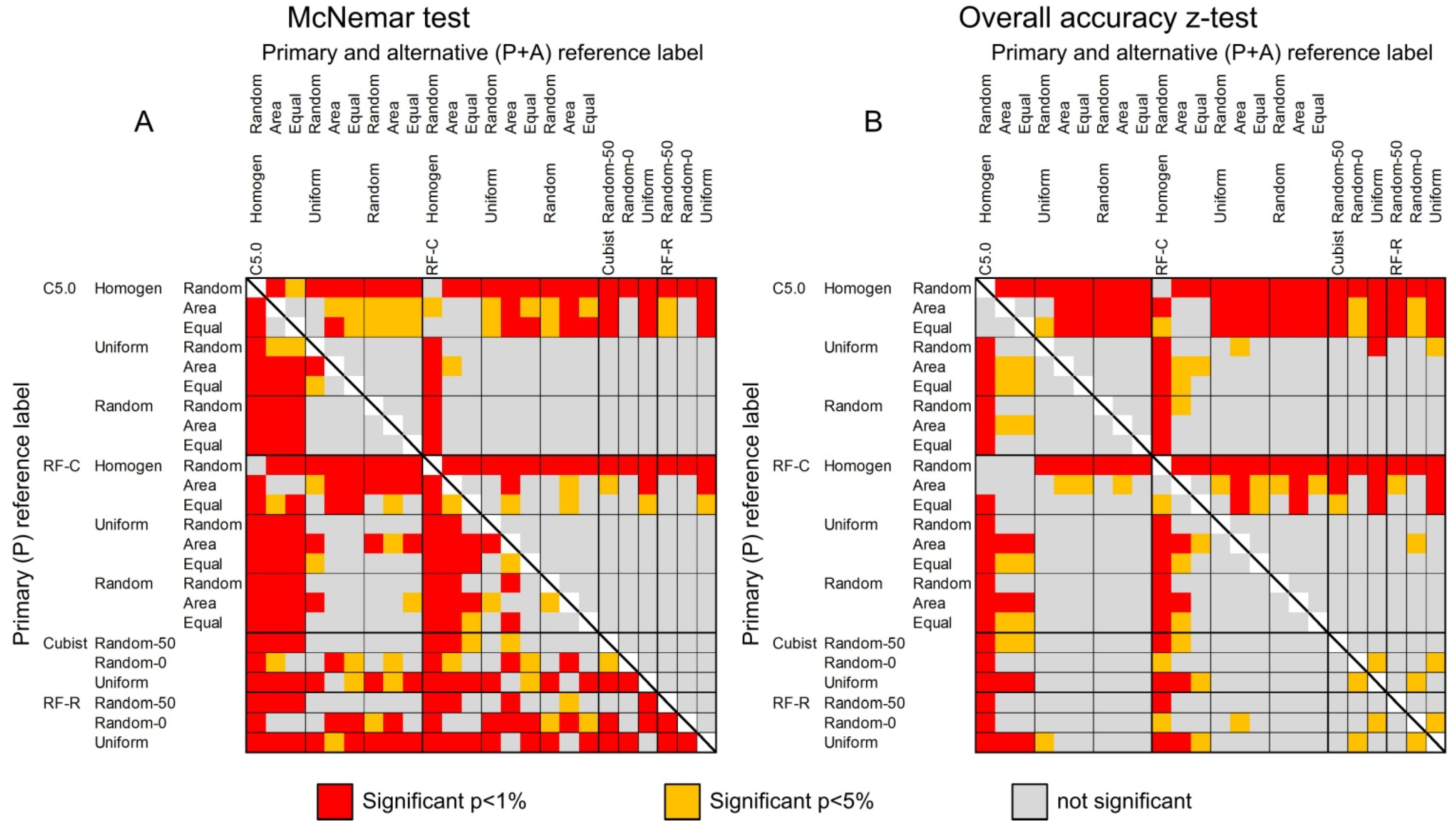
The differences in classification accuracies were statistically tested using McNemar test and Figure 4A depicts the statistically significant differences. In contrast to using only the primary reference label (lower-left triangle), there are less significant differences for assessments with the primary and alternative reference label (upper right triangle). Most obvious is that sampling homogeneous training data for classification trees almost always performs significantly worse (for actual accuracies see Table 9 and supplemental material). There are statistically significant differences between classification trees using heterogeneous training samples and regression trees, even though the differences in overall accuracies are low. This is due to the nature of the test, which aims at the number in differences of correctly and incorrectly classified reference samples between two classifications. The statistically significant differences in overall accuracies are shown in Figure 4B. Again, most notable is that classifications with homogeneous training samples perform significantly worse than all others. The main difference to McNemar test is that there are more statistically significant differences for the reference set using primary + alternative calls as correctly classified due to the higher range in overall accuracies (see also Table 9).

Figure 4. Statistical significance of difference in accuracies between (A) image classifications using McNemar test and (B) overall accuracies. Lower-left triangle shows results for the primary reference label, upper-right triangle for the primary and alternative reference label as correctly classified.

Figure 4. Statistical significance of difference in accuracies between (A) image classifications using McNemar test and (B) overall accuracies. Lower-left triangle shows results for the primary reference label, upper-right triangle for the primary and alternative reference label as correctly classified.

4.3.3. Class-Membership Assessment

The continuous reference derived from NLCD2006 is used for assessing class memberships across all classes using four statistics (Table 9): correlation coefficient (r), mean absolute difference (MAD), slope, and intercept (Int). Memberships from C5.0 show in general inferior results with lowest r and highest MAD compared to other tested algorithms. Homogeneous training data for classification trees are clearly inferior compared to heterogeneous training pixels (∆r = 0.11 and ∆MAD = 1.94%). Equal allocation between classes results in slightly lower correlation and higher MAD than random or area-proportional allocation. For regression trees, random allocation shows 0.07 higher correlations and a notably (4.9%) lower MAD than uniform sampling. Normalization only marginally improves correlation coefficients but the MAD decreases by 1.5%. Best results of classification trees were obtained for RF-C with area-proportional between-class sample allocation and randomly allocated heterogeneous samples (r = 0.83, MAD = 6.67%) which is almost as good as best results from regression trees with Cubist, random allocation of heterogeneous pixels with no minimum set and normalization r = 0.86 and MAD = 5.93%).

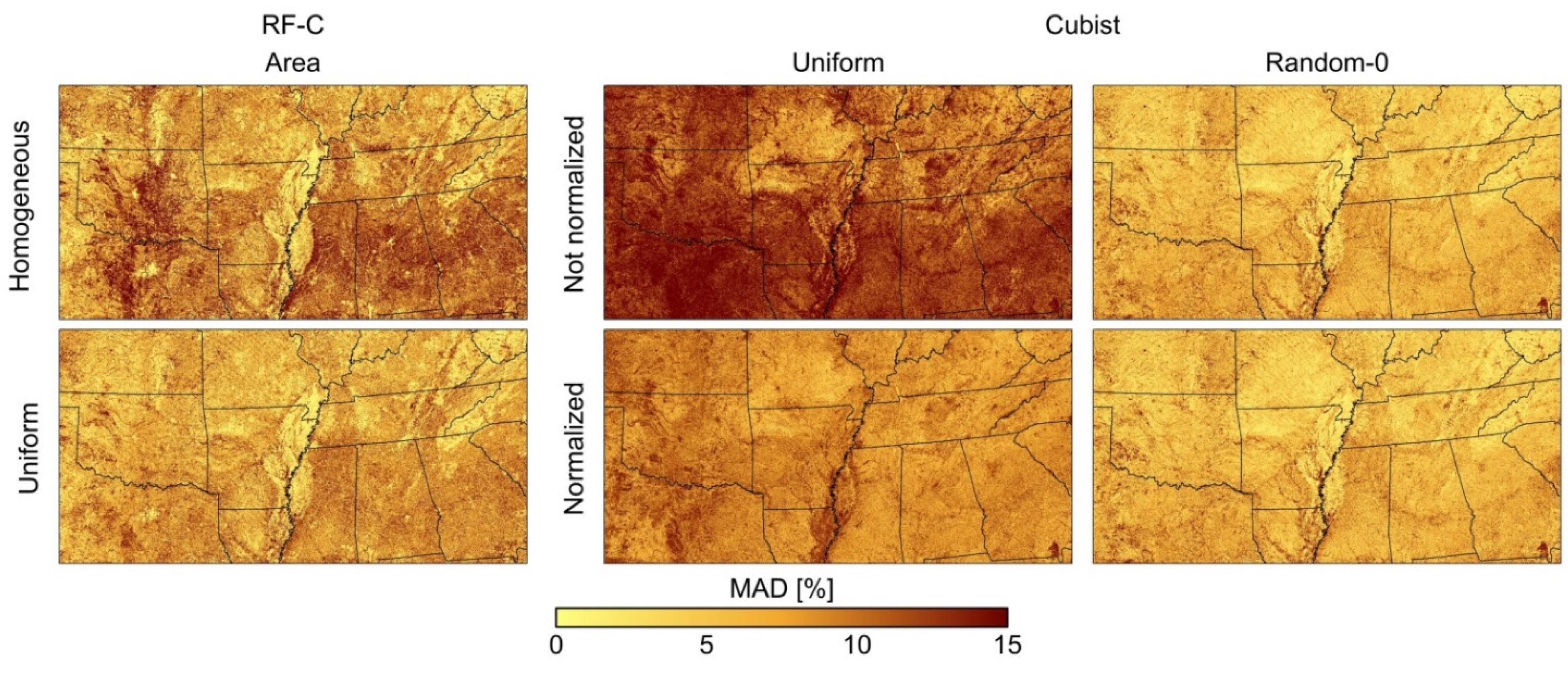
Figure 5 shows the spatial distribution of the MAD for which MAD was computed for each pixel individually. The figure only displays results for RF-C and Cubist; the spatial distribution of the error was similar for C5.0 and RF-R, respectively. For classification trees there are no spatial differences between among-class allocations (area-proportional allocation is shown), and there are no differences between allocations of heterogeneous pixels (uniform is displayed), which corresponds to the spatial patterns shown in Figure 3C. Allocating only homogeneous pixels for training shows notably higher errors in general and in particular for transitional zones from Deciduous forest to Evergreen forest in Mississippi, Alabama, and Georgia as well as transitions from Shrubland to Cultivated crops to Grassland in Texas and Oklahoma. Regression tree results with random allocation of heterogeneous pixels depict no differences among each other (Random-0 is depicted) for which normalization has no impact on the spatial distribution of errors. There are isolated areas with high errors, e.g., the Okefenokee Swamp in southeastern Georgia for which the membership values for class Wetland were underestimated. Uniform allocation depicts high MAD throughout the entire image, which decrease when normalization is applied.

Figure 5. Spatial mean absolute difference (MAD) of selected image sets of class memberships. Random forest classification (RF-C) with area-proportional sample allocation between classes and homogeneous and heterogeneous, uniformly allocated training pixels. Cubist with uniform and random allocation of heterogeneous training pixels and with and without normalization.

Figure 5. Spatial mean absolute difference (MAD) of selected image sets of class memberships. Random forest classification (RF-C) with area-proportional sample allocation between classes and homogeneous and heterogeneous, uniformly allocated training pixels. Cubist with uniform and random allocation of heterogeneous training pixels and with and without normalization.

Parameters of the regression line between reference and predicted values show generally better results for classification trees with higher slopes and lower intercepts compared to regression trees. RF-C with uniform allocation of heterogeneous training pixels shows highest slopes (0.92) and lowest intercept (0.82%). For regression trees, uniform allocation of heterogeneous pixels and no normalization indicates highest slope (0.86) for Cubist at the expense of a very high intercept with 11.71%; the lowest intercept of 2.56 was found for random sampling and no normalization.

4.4. Area Analysis

A second criterion for classifier performance and analysis of different sampling schemes is the similarity of area estimates. Table 9 depicts the total absolute difference between area proportions of the NLCD2006 map as reference and class membership or discrete maps expressed in million hectares and percent against the total study area. For instance, class-memberships of the C5.0 classification tree with homogeneous training pixels and random sample allocation between classes (first line in Table 9) shows a difference of 85.47 Mio ha or 52.76% to the NLCD2006 as reference.

Area differences from discrete maps for classification trees show no notable differences among algorithms (average of 24.30% for C5.0, 24.79% for RF-C) and a clearly better performance of heterogeneous pixel allocation (16.02%) compared to 41.59% for homogeneous pixels. For heterogeneous training pixels, equal allocation of samples between classes shows up to 2% lower differences than area-proportional allocation and 5%–8% lower than random allocation. For this sample allocation the C5.0 algorithm shows a slightly better result than RF-C. For regression trees Cubist shows slightly lower differences (average of 16.42%) than RF-R (17.78). Uniform allocation using Cubist shows lowest difference (9.46%), which is in line with better overall accuracies when measured with homogeneous test data (H = 100).

For membership estimates from classification trees, on average, there is no notable difference between C5.0 (20.83%) and RF-C (20.24%). Homogeneous training data show clearly inferior results with on average 39.90% difference compared to heterogeneous training pixels (10.85%). Area-proportional sample allocation of randomly sampled heterogeneous pixels yield best results with 3.93% total difference for RF-C. Memberships from regression trees show lower differences for Cubist (average 23.37%) than RF-R (29.45%). Random allocation (6.21%) clearly outperforms uniform sampling (66.82%). The table also indicates the importance of normalization (13.27%) because non-normalized results on average cannot correct the total area estimate (39.56%). For Cubist (RF-R), sampling with Random-50 estimated 110.0% (118.4%), Random-0 99.1% (105.6%) and Uniform 191.9% (209.8%) of the total area as compared to NLCD2006. Total areas of non-normalized results for random sampling are relatively close to the true total area, which is also the best result using Cubist with an absolute difference of 1.55%.

5. Discussion

5.1. Reference Data

The NLCD data set provides a unique opportunity for this study because it maps common land cover classes at 30 m spatial resolution in a consistent manner over a large region. The area chosen in this study includes various semi-natural and human-controlled landscapes with large and small patches as well as transitional environmental zones from dry to moist and temperate to sub-tropical climate, which is useful to test the effectiveness of different sampling schemes with discrete and continuous classifications.

This study used the projection and spatial registration of NLCD2006 [37,38,40] and instead re-projected MODIS data, because NLCD2006 was considered to be the reference for this study that should not be altered. During re-projection, MODIS cells were resampled from 926 m to 900 m and referenced to the cell location of NLCD so one MODIS cell is nested to 30 × 30 NLCD pixels. The quantitative analysis of spatial co-registration for ten selected Landsat images, used for NLCD mapping in 2006, showed near-to-perfect spatial correspondence with MODIS image composites, which allows direct comparison between 30 m cells in NLCD2006 to its corresponding 900 m MODIS pixel.

The classification accuracy of NLCD2006 with 16 original classes is 78% and class aggregation to level I with eight classes yields 84% overall accuracy [40]. In comparison, assessment of NLCD2006 for the southeastern United States with nine classes (Table 1) and coarsened to 900 m (Figure 3B) using the primary or primary and alternative reference samples resulted in 59.3% respective 72.9% overall accuracy. Major sources of error are Wetland, which was frequently confused with forests, also having the lowest accuracies in NLCD2006 [40], and Pasture versus Grassland, as two land-use forms of herbaceous cover. Despite the coarse resolution developed areas were classified well.

The potentially smallest unit to be mapped is the pixel area [58]. Applying a minimum mapping unit (MMU), that is the smallest area of contiguous pixels in the map, will remove isolated pixels. A “smart-eliminate algorithm” with eight-neighbor rule is applied to publically released 30 m NLCD2006 maps with MMUs of 5 pixels (0.45 ha) for developed classes, 32 pixels (2.88 ha) for classes pasture/hay and cultivated crops, and 12 pixels (1.08 ha) for all other classes [37]. The corresponding potential errors for each MODIS pixel (MMU (ha) × 100/81 ha) introduced by these minimum object sizes are 0.55%, 3.55%, and 1.33%, respectively. The error is directly proportional to the ratio between MMUs of NLCD2006 and a MODIS cell with 81 ha (900 m spatial resolution), which was the main reason for choosing the MCD43B4 data instead of MCD43A4 data with 463 m (resampled to 450 m, 20.25 ha pixel area). It should be noted that NLCD is the best regional fine resolution data source available for the analysis performed in this study. Therefore NLCD2006 was used as a high spatial resolution source to allocate training samples for MODIS image classification, for assessment of class memberships, and reference of areas for each land cover class. As decision tree classifiers can deal with some level of error in the training data the impact of error on the classification is considered to be low, but the impact on error statistics for continuous map assessment cannot be estimated.

5.2. Sample Allocation for Training Data

This study assessed different allocation schemes for training decision trees from a high spatial resolution map (NLCD2006) employing various accuracy measures for discrete and continuous maps and difference in area. Other issues such as sample size or feature set dimensionality were not addressed because there is ample literature on this subject [28,30,59]. The total size of 5400 samples for classification and regression was deemed sufficient; a training sample size set of approximately 0.25% of the study area is realistic for many applied remote sensing studies. In addition, various sample allocations ensured a minimum size of 50 samples per class or sample bin, which corresponds to approximately 1% of all samples. The actual number of 5400 training samples should not be generalized to other studies, but was deemed useful here because it is divisible without remainder by the number of classes (9) and for the number of bins (6 and 12), which eased sample allocation and data processing in this study.

For classification trees, heterogeneous training pixels are recommended and if possible uniform allocation should be preferred because of slopes closer to 1 and intercepts closer to 0. Even though previous studies for very small areas suggested that heterogeneous training data could improve discrete classifications [24,35,37], results of this study demonstrate for first time that they have a better performance for membership estimates over a large and diverse area.

Sample size balance between classes is a controversial topic in image classification [7,26,27,30,32]. In particular classification trees may suffer from unbalanced sample sizes [33], because in their standard form the class with the highest number of samples determines the class label. On the other hand, it could be argued that classes with multimodal frequency distributions, e.g., cropland with different crop types and growing cycles, should have more samples to be accurately represented in the classifier than a spectrally and temporally well-defined class such as water. This study tested random, area-proportional and equal sample allocation between all classes. Area-proportional allocation is recommended because of best area estimations and similarly high accuracy measures as random allocation. This result corresponds with the hypothesis that classes with a large area proportion and thus a higher probability of multiple modes in the feature space require more samples than classes with a small area proportion [7,27].

At first sight, regression methods seem more suitable for estimating memberships because their predictions intrinsically derive fractional estimates [24,34,53,60], but the additional step of normalization is necessary to obtain correct area totals. In general random allocation of heterogeneous samples is recommended for which normalization may not even be necessary, but is still recommended for all regression results as differing area totals may complicate further data analysis. Uniform allocation may be useful for discrete maps with better area estimates and accuracies similar to random allocation. The reason for testing uniform allocation was based on the hypothesis that a higher number of training pixels with high homogeneity may improve the prediction of high membership values, which is commonly underrepresented in random allocation (e.g., Table 7).

5.3. Classification Methods

Membership estimation from classification trees requires multiple iterations. For random forest classification this was realized with 1000 iterations and randomized selection of features and samples [48]. For C5.0 a process described in Colditz et al. [43] computes the class proportion from samples of each leaf and averages the memberships of all boosted trees. Alternative possibilities to estimate class memberships are suggested in McIver and Friedl [61].

There are notable differences between results from classification trees (C5.0, RF-C) versus regression trees (Cubist, RF-R) and the performance of each algorithm depends on appropriate training data allocation. Regression trees depict higher accuracies and lower area differences than classification tree results. This, however, comes at the expense of lower slopes and higher intercepts, which affects the dynamic range of predicted membership values. The selection of a decision tree type should also include the computational costs such as time and storage. Classification trees only require one sampling process for all classes with one tree model, which may be iterated to derive class memberships. The complexity for regression trees increments with the number of classes for which each requires a separate sampling process and tree model.

With respect to the actual algorithm the differences are small, but from the tested algorithms RF-C should be preferred for classification trees and Cubist for regression. The main reason for the better performance of RF-C is likely related to the higher number of iterations (1000) as compared to 10-folded boosting with C5.0. It should also be noted that RF-C was executed in the most basic way and there are multiple options to improve results, e.g., by outlier removal and a priori sample stratification [50]. The better performance of Cubist as compared to RF-R likely relates to the generation of a rule set and formulation of linear equations with specific weights for each input variable. In addition, Cubist results can be improved, e.g., by extrapolation beyond training data range which could increase the slopes of regression models and thus better estimate the full dynamic range.

Many studies compare classification results among different conceptual approaches to classify remote sensing data such as Maximum Likelihood classification (MCL), Artificial Neural Networks, Decision trees, and Support Vectors [10,16,17]. This study only focused on decision trees, because each conceptual approach has certain needs with respect to feature sets and training data and thus results are likely biased towards one algorithm. For instance, multivariate statistics for MLC should include statistical tests for Gaussian frequency distributions and in case of multimodal frequency distributions training samples should be separated in different groups. Even in this study different sample allocation strategies had to be used to train classification trees, e.g., with respect to between-class sample balance, as compared to regression trees, for which this is not an issue. Therefore, results of this study can only be generalized for decision-tree models.

6. Conclusions

This study tested several sampling methods for discrete classification and class membership estimation (i.e., continuous land cover) using decision-tree methods. It employed an annual time series of spectral bands of MODIS data at 900 m spatial resolution and a subset of the 2006 National Land Cover Database as wall-to-wall finer resolution reference map from which training samples were allocated. Spatial co-registration was ensued with baseline Landsat data that also served as response data for discrete map assessment. There are three main conclusions:

(1)

Regression trees show higher accuracies and lower differences in expected area but classification trees better predict the full dynamic range of values. For tested regression tree methods, results of Cubist are better than random forest regression. Random forest classification performs better than C5.0 with boosted trees.

(2)

For classification trees, heterogeneous training data perform clearly better than homogeneous pixels for both, discrete and continuous land cover mapping. Uniform allocation of heterogeneous pixels is slightly better than random allocation. For between-class sample allocation area-proportional training data allocation is recommended.

(3)

For regression trees, normalization is imperative to correctly estimate the total area of class memberships. Random allocation is very important for estimating class memberships. A uniform sampling structure can be recommended for deriving discrete maps.

This study only focused on one study area, the southeastern United States. Further tests in other regions of the world and with different data sets and scales, e.g., 30 m image classification trained with 1 m reference data, will be needed to confirm and generalize its results.

References

- Homer, C.; Dewitz, J.; Fry, J.; Coan, M.; Hossain, N.; Larson, C.; Herold, N.; McKerrow, A.; VanDriel, J.N.; Wickham, J. Completion of the 2001 National Land Cover Database for the conterminous United States. Photogramm. Eng. Remote Sens. 2007, 73, 337–341. [Google Scholar]
- Thompsom, M. A standard land-cover classification scheme for remote-sensing applications in South Africa. S. Afr. J. Sci. 1996, 92, 34–42. [Google Scholar]
- Feranec, J.; Jaffraini, G.; Soukup, T.; Hazeu, G. Determining changes and flows in European landscapes 1990–2000 using CORINE land cover data. Appl. Geogr. 2010, 30, 19–35. [Google Scholar] [CrossRef]
- Hansen, M.C.; Popatov, P.V.; Moore, R.; Hancher, M.; Turubanova, S.A.; Tyukavina, A.; Thau, D.; Stehman, S.V.; Goetz, S.J.; Loveland, T.R.; et al. High resolution global maps of 21st-century forest cover change. Science 2013, 342, 850–853. [Google Scholar] [CrossRef] [PubMed]
- Townshend, J.R.; Masek, J.G.; Huang, C.; Vermote, E.F.; Gao, F.; Channan, S.; Sexton, J.O.; Feng, M.; Narasimhan, R.; Kim, D.; et al. Global characterization and monitoring of forest cover using Landsat data: Opportunities and challenges. Int. J. Digit. Earth 2012, 5, 373–397. [Google Scholar] [CrossRef]
- Gong, P.; Wang, J.; Yu, L.; Zhao, Y.C.; Zhao, Y.Y.; Liang, L.; Niu, Z.; Huang, X.; Fu, H.; Liu, S.; et al. Finer resolution observation and monitoring of global land cover: First mapping results with Landsat TM and ETM+ data. Int. J. Remote Sens. 2013, 34, 2607–2654. [Google Scholar] [CrossRef]
- Blanco, P.D.; Colditz, R.R.; López Saldaña, G.; Hardtke, L.A.; Llamas, R.M.; Mari, N.A.; Fischer, A.; Caride, C.; Aceñolaza, P.G.; del Valle, H.F.; et al. A land cover map of Latin America and the Caribbean in the framework of the SERENA project. Remote Sens. Environ. 2013, 132, 13–31. [Google Scholar] [CrossRef]
- Friedl, M.A.; McIver, D.K.; Hodges, J.C.F.; Zhang, X.Y.; Muchoney, D.; Strahler, A.H.; Woodcock, C.E.; Gopal, S.; Schneider, A.; Cooper, A.; et al. Global land cover mapping from MODIS: Algorithms and early results. Remote Sens. Environ. 2002, 83, 287–302. [Google Scholar] [CrossRef]
- De Fries, R.S.; Hansen, M.C.; Townshend, J.R.G.; Sohlberg, R. Global land cover classifications at 8 km spatial resolution: The use of training data derived from Landsat imagery in decision tree classifiers. Int. J. Remote Sens. 1998, 19, 3141–3168. [Google Scholar] [CrossRef]
- Fernandes, R.; Fraser, R.; Latifovic, R.; Cihlar, J.; Beaubien, J.; Du, Y. Approaches to fractional land cover and continuous field mapping: A comparative assessment over the BOREAS study region. Remote Sens. Environ. 2004, 89, 234–251. [Google Scholar] [CrossRef]
- Löw, F.; Duveiller, G. Defining the spatial resolution requirements for crop identification using optical remote sensing. Remote Sens. 2014, 6, 9034–9063. [Google Scholar] [CrossRef]
- Hansen, M.C.; DeFries, R.S.; Townshend, J.R.G.; Sohlberg, R.; Dimiceli, C.; Carroll, M. Towards an operational MODIS continuous field of percent tree cover algorithm: Examples using AVHRR and MODIS data. Remote Sens. Environ. 2002, 83, 303–319. [Google Scholar] [CrossRef]
- Moody, A.; Woodcock, C.E. Scale-dependent errors in the estimation of land-cover proportions: Implications for Global Land-Cover Datasets. Photogramm. Eng. Remote Sens. 1994, 60, 584–594. [Google Scholar]
- Treitz, P.; Howarth, P. High spatial resolution remote sensing data for forest ecosystem classification: An examination of spatial scale. Remote Sens. Environ. 2000, 72, 268–289. [Google Scholar] [CrossRef]
- Fisher, P.F. Remote sensing of land cover classes as type 2 fuzzy sets. Remote Sens. Environ. 2010, 114, 309–321. [Google Scholar] [CrossRef]
- Okujeni, A.; van der Linden, S.; Jakimow, B.; Rabe, A.; Verrelst, J.; Hostert, P. A comparison of advanced regression algorithms for quantifying urban land cover. Remote Sens. 2014, 6, 6324–6346. [Google Scholar] [CrossRef]
- Li, C.; Wang, J.; Wang, L.; Hu, L.; Gong, P. Comparison of classification algorithms and training sample sizes in urban land classification with Landsat thematic mapper imagery. Remote Sens. 2014, 6, 964–983. [Google Scholar] [CrossRef]
- Friedl, M.A.; Brodley, C.E.; Strahler, A.H. Maximizing land cover classification accuracies produced by decision trees at continental to global scales. IEEE Trans. Geosci. Remote Sens. 1999, 37, 969–977. [Google Scholar] [CrossRef]
- DeFries, R.S.; Townshend, J.R.G. NDVI derived land cover classifications at a global scale. Int. J. Remote Sens. 1994, 15, 3567–3586. [Google Scholar] [CrossRef]
- Gopal, S.; Woodcock, C.E.; Strahler, A.H. Fuzzy neural network classification of global land cover from a 1° AVHRR Data Set. Remote Sens. Environ. 1999, 67, 230–243. [Google Scholar] [CrossRef]
- Clark, M.L.; Aide, T.M.; Riner, G. Land change for all municipalities in Latin America and the Caribbean assessed from 250-m MODIS imagery (2001–2010). Remote Sens. Environ. 2012, 126, 84–103. [Google Scholar] [CrossRef]
- Friedl, M.A.; Sulla-Menashe, D.; Tan, B.; Schneider, A.; Ramankutty, N.; Sibley, A.; Huang, X. MODIS Collection 5 global land cover: Algorithm refinements and characterization of new datasets. Remote Sens. Environ. 2010, 114, 168–182. [Google Scholar] [CrossRef]
- Latifovic, R.; Homer, C.; Ressl, R.; Pouliot, D.; Hossain, S.N.; Colditz, R.R.; Olthof, I.; Giri, C.P.; Victoria, A. North American land-change monitoring system. In Remote Sensing of Land Use and Land Cover: Principles and Applications; Giri, C.P., Ed.; CRC/Taylor & Francis: Boca Raton, FL, USA, 2012; pp. 303–324. [Google Scholar]
- Xu, M.; Watanachaturaporn, P.; Varshney, P.K.; Arora, M.K. Decision tree regression for soft classification of remote sensing data. Remote Sens. Environ. 2005, 97, 322–336. [Google Scholar] [CrossRef]
- Yang, L.; Xian, G.; Klaver, J.M.; Deal, B. Urban land-cover change detection through sub-pixel imperviousness mapping using remotely sensed data. Photogramm. Eng. Remote Sens. 2003, 69, 1003–1010. [Google Scholar] [CrossRef]
- Borak, J.S.; Strahler, A.H. Feature selection and land cover classification of a MODIS-like data set for a semiarid environment. Int. J. Remote Sens. 1999, 20, 919–938. [Google Scholar] [CrossRef]
- Colditz, R.R.; Schmidt, M.; Conrad, C.; Hansen, M.C.; Dech, S. Land cover classification with coarse spatial resolution data to derive continuous and discrete maps for complex regions. Remote Sens. Environ. 2011, 115, 3264–3275. [Google Scholar] [CrossRef]
- Conrad, C.; Colditz, R.R.; Dech, S.; Klein, D.; Vlek, P.L.G. Temporal segmentation of MODIS time series for improving crop classification in Central Asian irrigation systems. Int. J. Remote Sens. 2011, 32, 8763–8778. [Google Scholar] [CrossRef]
- Pouliot, D.; Latifovic, R.; Fernandes, R.; Olthof, I. Evaluation of annual forest disturbance monitoring using a static decision tree approach and 250 m MODIS data. Remote Sens. Environ. 2009, 113, 1749–1759. [Google Scholar] [CrossRef]
- Pal, M.; Mather, P.M. An assessment of the effectiveness of decision tree methods for land cover classification. Remote Sens. Environ. 2003, 86, 554–565. [Google Scholar] [CrossRef]
- Radoux, J.; Lamarche, C.; van Bogaert, E.; Bontemps, S.; Brockmann, C.; Defourny, P. Automated training sample extraction for global land cover mapping. Remote Sens. 2014, 6, 3965–3987. [Google Scholar] [CrossRef]
- Jin, H.; Stehman, S.V.; Mountrakis, G. Assessing the impact of training sample extraction on accuracy of an urban classification: A case study in Denver, Colorado. Int. J. Remote Sens. 2014, 35, 2067–2081. [Google Scholar]
- Hansen, M.C.; DeFries, R.S.; Townshend, J.R.G.; Sohlberg, R. Global land cover classification at 1 km spatial resolution using a classification tree approach. Int. J. Remote Sens. 2000, 21, 1331–1364. [Google Scholar] [CrossRef]
- Im, J.; Lu, Z.; Rhee, J.; Quackenbush, L. Impervious surface quantification using a synthesis of artificial immune networks and decision/regression trees from multi-sensor data. Remote Sens. Environ. 2012, 117, 102–113. [Google Scholar] [CrossRef]
- Foody, G.M.; Mathur, A. The use of small training sets containing mixed pixels for accurate hard image classification: Training on mixed spectral responses for classification by a SVM. Remote Sens. Environ. 2006, 103, 179–189. [Google Scholar] [CrossRef]
- Hansen, M.C. Classification trees and mixed pixel training data. In Remote Sensing of Land Use and Land Cover: Principles and Applications; Giri, C.P., Ed.; CRC/Taylor & Francis: Boca Raton, FL, USA, 2012; pp. 127–136. [Google Scholar]
- Fry, J.A.; Xiang, G.; Jin, S.; Dewitz, J.A.; Homer, C.G.; Yang, L.; Barnes, C.A.; Herold, N.D.; Wickham, J.D. National Land Cover Database for the conterminous United States. Photogramm. Eng. Remote Sens. 2011, 77, 859–864. [Google Scholar]
- Xian, G.; Homer, C.; Fry, J. Updating the 2001 National Land Cover Database land cover classification to 2006 by using Landsat imagery change detection methods. Remote Sens. Environ. 2009, 113, 1133–1147. [Google Scholar] [CrossRef]
- Jin, S.; Yang, L.; Danielson, P.; Homer, C.; Fry, J.; Xian, G. A comprehensive change detection method for updating the National Land Cover Database to circa 2011. Remote Sens. Environ. 2013, 132, 159–175. [Google Scholar] [CrossRef]
- Wickham, J.D.; Stehman, S.V.; Gass, L.; Dewitz, J.; Fry, J.A.; Wade, T.G. Accuracy assessment of NLCD2006 land cover and impervious surface. Remote Sens. Environ. 2013, 130, 294–304. [Google Scholar] [CrossRef]
- Schaaf, C.B.; Gao, F.; Strahler, A.H.; Lucht, W.; Li, X.; Tsang, T.; Strugnell, N.C.; Zhang, X.; Jin, Y.; Muller, J.-P.; et al. First operational BRDF, albedo nadir reflectance products from MODIS. Remote Sens. Environ. 2002, 83, 135–148. [Google Scholar] [CrossRef]
- Schaaf, C.; Liu, J.; Gao, F.; Jiao, Z.; Shuai, Y.; Strahler, A. Collection 005 Change Summary for MODIS BRDF/Albedo (MCD43) Algorithms; 2006. Available online: http://landweb.nascom.nasa.gov/QA_WWW/forPage/C005_Change_BRDF.pdf (accessed on 22 June 2015).
- Colditz, R.R.; López Saldaña, G.; Maeda, P.; Argumedo Espinoza, J.; Meneses Tovar, C.; Victoria Hernández, A.; Zermeño Benítez, C.; Cruz López, I.; Ressl, R. Generation and analysis of the 2005 land cover map for Mexico using 250 m MODIS data. Remote Sens. Environ. 2012, 123, 541–552. [Google Scholar] [CrossRef]
- Colditz, R.R.; Conrad, C.; Wehrmann, T.; Schmidt, M.; Dech, S. TiSeG: A flexible software tool for time-series generation of MODIS data utilizing the quality assessment science data set. IEEE Trans. Geosci. Remote Sens. 2008, 46, 3296–3308. [Google Scholar] [CrossRef]
- Colditz, R.R.; Acosta-Velázquez, J.; Díaz Gallegos, J.; Vázquez Lule, A.; Rodríguez Zúñiga, M.; Maeda, P.; Cruz López, M.; Ressl, R. Potential effects in multiresolution post-classification change detection. Int. J. Remote Sens. 2012, 33, 6426–6445. [Google Scholar] [CrossRef]
- Breiman, L.; Friedman, J.H.; Olshen, R.A.; Stone, C.J. Classification and Regression Trees; Wadsworth Statistics/Probability; Chapman and Hall/CRC: Boca Raton, FL, USA, 1984. [Google Scholar]
- Friedl, M.A.; Brodley, C.E. Decision tree classification of land cover from remotely sensed data. Remote Sens. Environ. 1997, 61, 399–409. [Google Scholar] [CrossRef]
- Breiman, L. Random forests. Mach. Learn. 2001, 45, 5–32. [Google Scholar] [CrossRef]
- Quinlan, J.R. C4.5: Programs for Machine Learning; Morgan Kaufmann Publishers: San Francisco, CA, USA, 1993. [Google Scholar]
- Liaw, A.; Wiener, M. Classification and regression by random forest. R News 2002, 2, 18–22. [Google Scholar]
- Quinlan, J.R. Learning with continuous classes. In Proceedings of the 5th Australian Joint Conference on Artificial Intelligence, Hobart, TAS, Australia, 16–18 November 1992; pp. 343–348.
- Quinlan, J.R. Combining instance-based and model-based learning. In Proceedings of the Tenth International Conference, University of Massachusetts, Amherst, MA, USA, 27–29 June 1993; pp. 236–243.
- Walton, J.T. Subpixel urban land cover estimation: Comparing cubist, random forests, and support vector regression. Photogramm. Eng. Remote Sens. 2008, 74, 1213–1222. [Google Scholar] [CrossRef]
- Xian, G.; Homer, C. Updating the 2001 National Land Cover Database Impervious Surface Products to 2006 using Landsat imagery change detection methods. Remote Sens. Environ. 2010, 114, 1676–1686. [Google Scholar] [CrossRef]
- Stehman, S.V.; Foody, G.M. Accuracy assessment. In The SAGE Handbook of Remote Sensing; Warner, T.A., Nellis, M.D., Foody, G.M., Eds.; SAGE Publications Ltd.: Thousand Oaks, CA, USA, 2009; pp. 297–311. [Google Scholar]
- Gao, Y.; Mas, J.-F.; Maathuis, B.H.P.; Zhang, X.; van Dijk, P.M. Comparison of pixel-based and object-oriented image classification approaches—A case study in a coal fire area, Wuda, Inner Mongolia, China. Int. J. Remote Sens. 2006, 27, 4039–4055. [Google Scholar]
- Foody, G.M. Thematic map comparison: Evaluating the statistical significance of differences in classification accuracy. Photogramm. Eng. Remote Sens. 2004, 70, 627–633. [Google Scholar] [CrossRef]
- Knight, J.F.; Lunetta, R.S. An Experimental assessment of minimum mapping unit size. IEEE Trans. Geosci. Remote Sens. 2003, 41, 2132–2134. [Google Scholar] [CrossRef]
- Hüttich, C.; Gessner, U.; Herold, M.; Strohbach, B.J.; Schmidt, M.; Keil, M.; Dech, S. On the suitability of MODIS time series metrics to map vegetation types in dry Savanna ecosystems: A case study in the Kalahari of NE Namibia. Remote Sens. 2009, 1, 620–643. [Google Scholar] [CrossRef]
- Johnson, D.M. An assessment of pre and within-season remotely sensed variables for forecasting corn and soybean yields in the United States. Remote Sens. Environ. 2014, 141, 116–128. [Google Scholar] [CrossRef]
- McIver, D.K.; Friedl, M.A. Estimating pixel-scale land cover classification confidence using nonparametric machine learning methods. IEEE Trans. Geosci. Remote Sens. 2001, 39, 1959–1968. [Google Scholar] [CrossRef]
© 2015 by the authors; licensee MDPI, Basel, Switzerland. This article is an open access article distributed under the terms and conditions of the Creative Commons Attribution license (http://creativecommons.org/licenses/by/4.0/).