Using Octrees to Detect Changes to Buildings and Trees in the Urban Environment from Airborne LiDAR Data

Abstract

Change detection is a major issue for urban area monitoring. In this paper, a new three-step point-based method for detecting changes to buildings and trees using airborne light detection and ranging (LiDAR) data is proposed. First, the airborne LiDAR data from two dates are accurately registered using the iterative closest point algorithm, and a progressive triangulated irregular network densification filtering algorithm is used to separate ground points from non-ground points. Second, an octree is generated from the non-ground points to store and index the irregularly-distributed LiDAR points. Finally, by comparing the LiDAR points from two dates and using the AutoClust algorithm, those areas of buildings and trees in the urban environment that have changed are determined effectively and efficiently. The key contributions of this approach are the development of a point-based method to effectively solve the problem of objects at different scales, and the establishment of rules to detect changes in buildings and trees to urban areas, enabling the use of the point-based method over large areas. To evaluate the proposed method, a series of experiments using aerial images are conducted. The results demonstrate that satisfactory performance can be obtained using the proposed approach.

1. Introduction

The detection of changes in the urban environment is becoming increasingly important for land management, the identification of illegal buildings, monitoring urban growth, urban landscape pattern analysis, and updating geographic information databases. As manual image interpretation and vectorization are time-consuming and expensive, automatic and semi-automatic change detection procedures are of considerable interest [1]. In particular, developing countries such as China and India, where numerous new buildings are constructed every year, urgently require approaches that can rapidly and automatically detect changes to urban building patterns.

Over recent decades, several automatic methods have been proposed that detect changes in the urban environment using remote sensing images [2,3,4]. At present, the main technique is to use multi-temporal very-high-resolution (VHR) satellite images to detect urban change [5], as the spectral information in these images is useful for this purpose. Change detection methodologies based on satellite images include both the pixel- [6,7] and object-based [4,8] approaches. However, methods based on VHR images with only 2D information can suffer from spectral variation. This makes image-based change detection difficult. Using images to detect change, image registration and multi-temporal radiometric corrections are perhaps the most important and indispensable steps [5]. Higher registration accuracy becomes more important when data are from different sensors and at different resolutions. Additionally, the effects of radiation differences must be minimized. Therefore, the change detection methods based on images can become somewhat complex.

Airborne light detection and ranging (LiDAR) technology has enjoyed rapid developments and has found applications in various fields [9,10,11,12]. Thus, airborne LiDAR technology presents a new avenue for change detection. Airborne LiDAR equipment can obtain detailed 3D information about the ground surface with a high degree of automation; however, the massive number of irregularly-distributed points brings new challenges for the task of change detection. Therefore, fully utilizing the advantages of LiDAR points remains an important topic of research. Methods that use airborne LiDAR for change detection can be classified into two categories from data sources: airborne LiDAR data integrated with ancillary data, and only airborne LiDAR data.

In the first category, the airborne LiDAR data is integrated with existing vector maps or stereo/aerial imagery to detect changes in the urban environment. Some studies have generated digital surface models (DSMs) from airborne LiDAR data and digital aerial images for the automatic detection of buildings and changes [7,13]. Tian et al. [14] proposed a merging strategy to get minimum change regions of buildings and forest based on the DSMs from two dates. This method can be used for both forest and industrial areas, but is difficult to detect changes to trees in urban environments due to the fact that the urban trees are usually small and discrete. In addition to the DSMs-based methods, Chen et al. [15] developed a technique based on a double-threshold strategy to identify changes within 3D building models in the region of interest with the aid of LiDAR data, in which the double-threshold strategy was applied to effectively cope with the highly-sensitive thresholding often encountered when detecting the changes in buildings or trees. Matikainen et al. [16] proposed a segment-based classification approach using LiDAR data and aerial imagery to detect buildings. They compared the detected buildings with those shown on existing maps, and then updated the maps using the change information. A similar method has been reported in the literature [17]. Malpica et al. [18] applied a support vector machine classification algorithm to a combined satellite and laser dataset for the extraction of buildings and determined the changes from the classification results. In addition to the change detection of buildings, there are some studies to detect changes in forest or tree biomass [19,20]. Although airborne LiDAR data integrated with ancillary data can effectively detect changes in buildings and trees, there are some differences in terms of the data characteristics and attributes, and these serve to increase the difficulty of data fusion. In addition, the change detection methods in this category are often complex.

In the second category, in which airborne LiDAR data is the only input data, most existing studies transform the LiDAR points into a DSM, and detect changes by comparing the DSMs from two dates. Murakami et al. [21] employed multi-temporal airborne LiDAR data to detect changes in buildings by direct surface comparison. Similarly, Vu et al. [22] developed an automatic building change detection method based on LiDAR data from dense urban areas. Teo et al. [23] proposed a change detection method that uses multi-temporal interpolated LiDAR data, in which the changes in building types were determined via geometric analysis. Pang et al. [24] developed an object-oriented analysis for multi-temporal point cloud data to detect building changes. In addition to the DSM-based methods, Zhang et al. [25] introduced an anisotropic-weighted iterative closest point algorithm, which iteratively minimizes the sum of the squares of the distances between two point clouds, to determine spatial changes. Although this point-based method can accurately determine 3D displacements between two point clouds, it is hard to detect changes in buildings and trees in the urban environment due to that the change types of them are not distinguished from each other. On account of large data volumes and irregular distribution of airborne LiDAR data, some studies presented appropriate methods to detect changes to our urban areas based on octree data structures [26,27]. Barber et al. [28] determined the changed areas according to the comparison of nodes between two octrees constructed for LiDAR point clouds from different dates. However, these studies do not classify the type of change. Change detection in forests with multi-temporal airborne LiDAR data has been demonstrated recently [29,30]. Yu et al. [31] analyzed the potential of airborne LiDAR data for measuring changes to individual tree height growth in a boreal forest, which is based on minimizing the distances between treetops in the N-dimensional data space, and has a good change detection result.

The aforementioned studies have demonstrated that automatic change detection in urban environments is possible, and that relatively good results can be achieved. However, most existing studies are based on DSM to detect changes, with results that are highly dependent on the quality of the DSM [7]. In addition, these studies do not consider change detection of tree cover in urban environments, and relatively few researches have classified the type of change. Therefore, it seems that further research is needed to develop a useful automatic method. In particular, there is an urgent need for a method that can use airborne LiDAR data to simultaneously detect changes in buildings and trees in the urban environment.

In this paper, we present a point-based approach for detecting changes in building and tree coverage in the urban environment using airborne LiDAR data, and identify the precise type of change. Our point-based method can overcome the problem of objects at different scales, which usually limits the use of DSM-based methods, and is suited to multi-target change detection. In addition, the geometric locations of the changed areas are not altered using the point-based method. However, when detecting changes based on points over a large urban environment, computational efficiency must be considered. Thus, an octree is introduced to manage and index the LiDAR points, efficiently solving the problem of high memory consumption.

2. Methodology

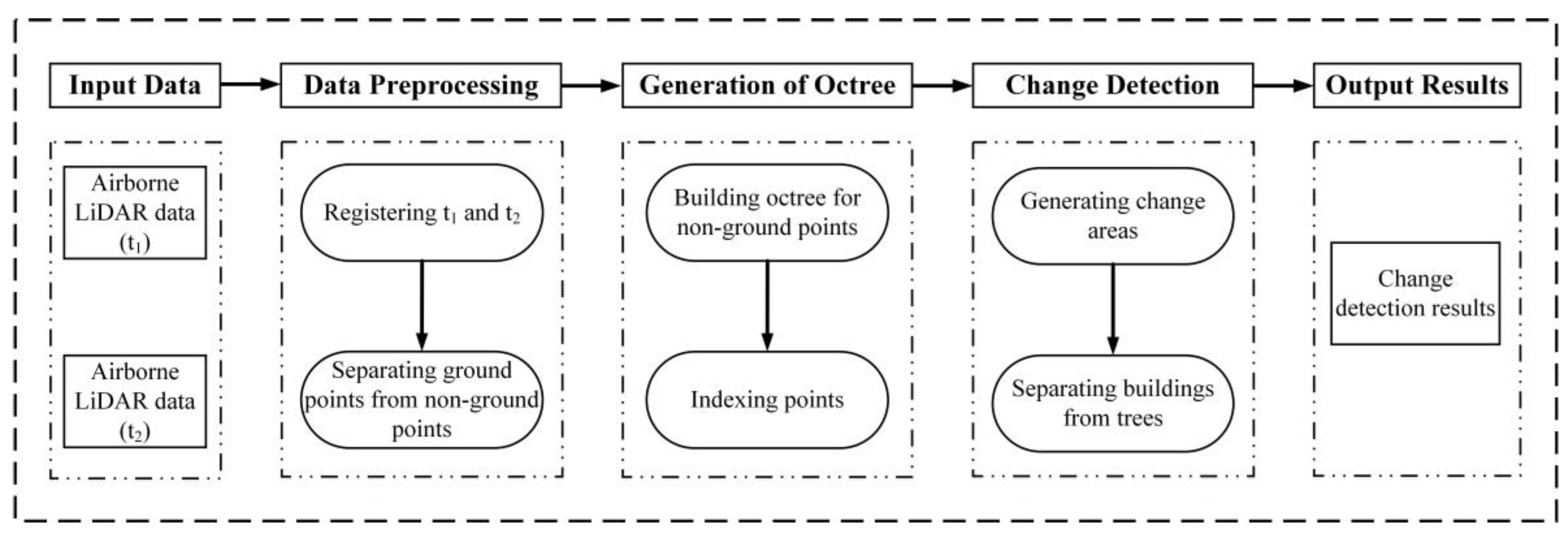
The proposed approach consists of three steps (see Figure 1). First, the original airborne LiDAR data are preprocessed to eliminate outliers, accurately register two airborne LiDAR point clouds, and separate ground points from non-ground points. Second, an octree is constructed from the non-ground points to accurately manage and index the LiDAR points. Finally, two airborne LiDAR point clouds are compared to determine the changed areas on the basis of the constructed octree. Those areas of buildings and trees that have changed can then be determined using a clustering method and a classification method.

Figure 1. Flowchart of the proposed approach.

Figure 1. Flowchart of the proposed approach.

2.1. Data Preprocessing

The proposed approach uses airborne LiDAR data to detect changes in buildings and trees. This requires airborne LiDAR point clouds from two dates. LiDAR point measurements mainly contain three components: bare ground, above-ground objects, and noise [32]. In practical applications, noise must first be eliminated to prevent it causing unpredictable errors in the experimental results. In the LiDAR point cloud, neighboring points have similar properties, whereas noise points will differ from their neighbors. Therefore, noise points can be removed by calculating the average μ and standard deviation value σ of the neighboring points. For a point p, when the Euclidean distance from p to a point q is less than the search radius r, the q is regarded as a neighboring point of p. The point p is regarded as an outlier when it is outside the range μ ± ασ, where α (we set 1.0 in this paper) depends on the size of the adjacent area.

After removing the noise, the airborne LiDAR point clouds from different dates should be registered accurately. Since the proposed approach is a point-based method, the registration of data from different dates has a direct effect on the results. Therefore, the data must be registered prior to the change detection. There are a number of accurate matching algorithms for airborne LiDAR point clouds [33,34,35]. The ICP algorithm, which uses least-squares to optimize the registration of point sets, is chosen to complete the data registration. The specific implementation of the ICP algorithm has been described in the literature [36].

In a LiDAR point cloud, the ground points represent 3D information from bare-earth terrain, and the non-ground points are the measurements from objects above the bare-earth terrain, such as buildings, trees, vehicles, etc. The proposed approach focuses on detecting changes in buildings and trees. To minimize the impact of the ground points, they are separated from the non-ground points in advance. There are numerous studies on filtering methods; in our method, a progressive triangulated irregular network (TIN) densification filtering algorithm is selected to filter out the ground points [37]. The separation of ground points and non-ground points consists of two steps: (1) Extracting ground points using the progressive TIN densification filtering algorithm; (2) Calculating the normalized height of each non-ground point.

In the process of establishing the TIN, we first set a search radius (2 m in this paper), and then select the point with the lowest height in each search area as the seed point for the initial ground TIN model. An iterative densification of the TIN is conducted. On the basis of the initial TIN model, the remaining lowest-height points, which satisfy the conditions of being joined to the ground set, are added to the initial TIN model in an iterative manner. When all LiDAR points have been traversed, the iteration is terminated. All LiDAR points representing the TIN nodes are ground points. The normalized height of each non-ground point is determined by calculating the distance from the non-ground point to the TIN, which eliminates the impact of the heights of the ground points, and allows us to focus on the heights of the buildings and trees themselves.

2.2. Generation of Octree for Non-Ground Points

After obtaining the non-ground points, changed regions can be identified by comparing the height values between the LiDAR data from two different dates. However, we should consider that change detection is often targeted at large areas. A point cloud captured by current LiDAR devices over a 2.5 km × 1.5 km area could consist of tens of millions of 3D points. This would make it very difficult to construct a 3D voxel grid system to index the desired points, as the process would exceed the memory constraints of mainstream computers. Therefore, it is very important to use a suitable data structure to store, manage, and index the raw points quickly and efficiently. In this paper, we introduce a spatial data structure known as an octree to store and index LiDAR points. In the past decade, several studies have implemented octrees for applications such as change detection, model generation, roof detection, point cloud visualization, and so on [26,27,28,38,39,40]. Octrees are a tree structure that can be used to index 3D data, and are very useful for space decompositions. They are a generalization of binary trees and quadtrees, which store 1D and 2D data, respectively [39]. Constructing an octree for large amounts of unorganized point cloud data will speed up the indexing of points. In the following subsections, we detail the process of establishing the octree and indexing the LiDAR points.

2.2.1. Octree Construction

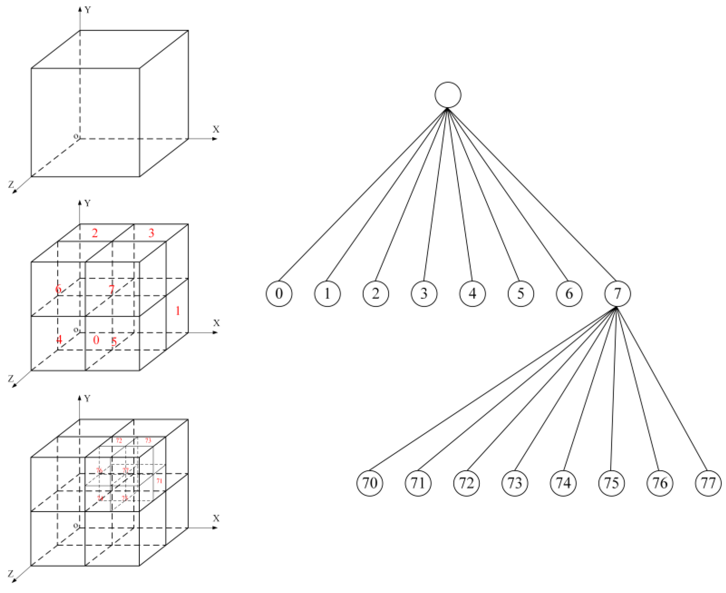
The processes of octree construction are similar to that in the literature [38,39]. First, the bounding box of the point cloud is computed and the root node, i.e., the first node, is initialized. The subsequent subdivision of an octree is conducted, where a node is subdivided into eight smaller nodes. Each node is described by its geometry and address. The geometry is defined by the coordinates of the node center. Each node in the octree structure has an address that reflects the relationship between adjacent nodes, and the path from the current node to its parent nodes, which is represented by a string of integers (see Figure 2 and Figure 3).

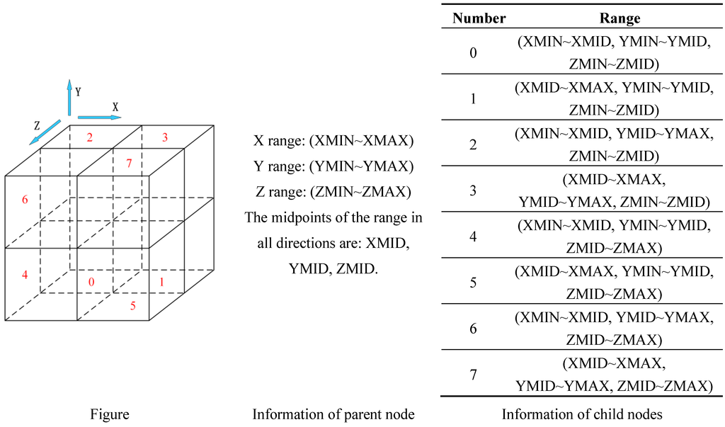
Figure 2. The division of spacein an octree.

Figure 2. The division of spacein an octree.

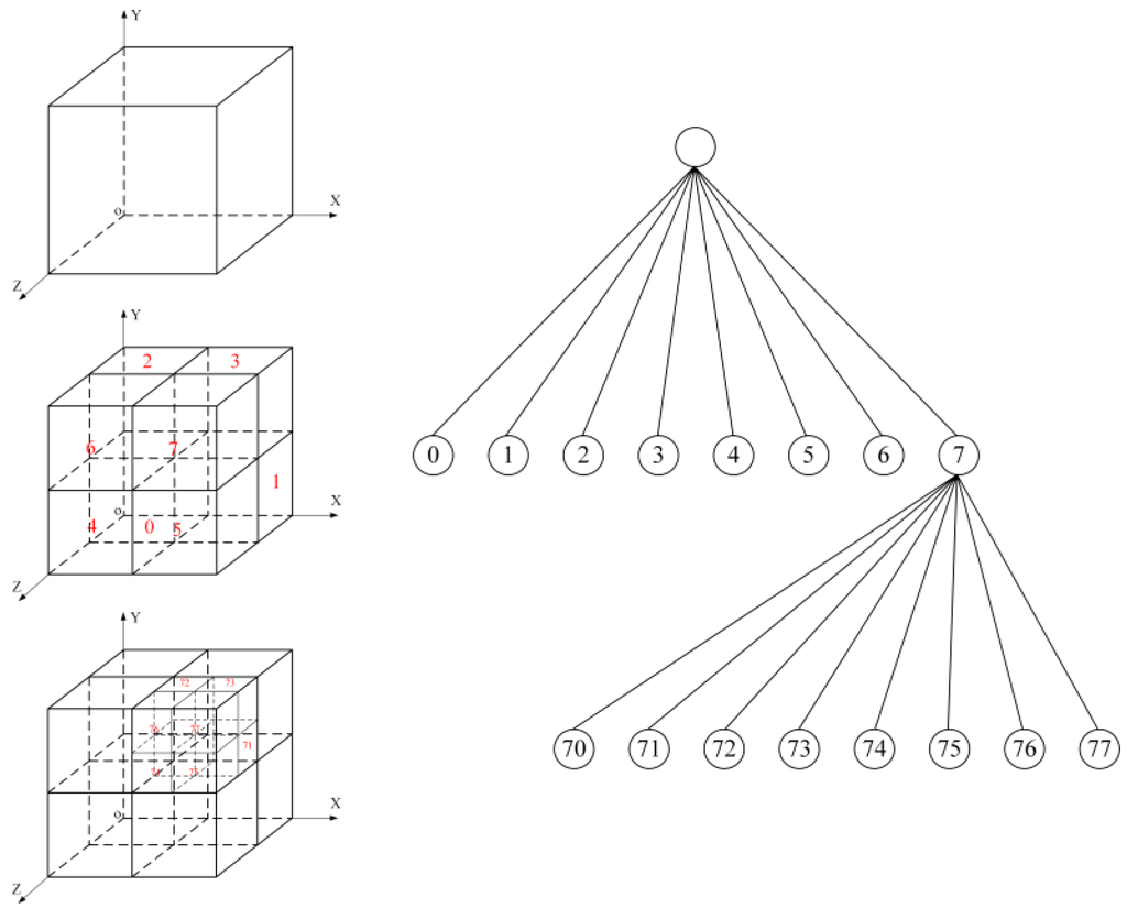
Figure 3. Octree presentation.

Figure 3. Octree presentation.

Selecting an appropriate termination criterion is crucial to an octree. In this study, both a minimal node size and a minimal number of points are defined as terminal criteria. The subdivision of space is terminated when a node meets the minimal threshold of points, even if the minimal node size has not been reached. A complete iteration process constructs the whole octree and a list of points is stored in each occupied leaf.

2.2.2. Indexing Points Based on Octree

The key to an efficient traversal to the leaf node containing the requiring points is the order in which the child nodes are visited. The 3D coordinates of a given query point p determine the leaf node to which it belongs. According to predefined rules, the neighboring points of p can then be selected. Without building an octree, finding the desired points would require an iteration over the entire dataset. In this paper, points within a radius of r are selected for further calculation. Therefore, determining the size of r and the minimal node is an important step in obtaining appropriate points for detecting changes in buildings and trees. In our test, r is 1 m and the minimal node size is 2 m. When the leaf node containing query point p has been confirmed, all points within last leaf node and its neighboring leaf nodes are selected as the initial points. The distances from the initial points to the query point are calculated to identify those points within a distance of r.

2.3. Change Detection Based on Octree

We now describe how to determine which areas have changed. First, because change detection in urban areas usually classifies points as either changed or unchanged, we define several change types based on regional attributes. Table 1 shows the categories of change types: new building, changed building, demolished building, new tree, and felled tree. In this study, the changed trees are not considered. This is mainly because, over a vegetative cycle of several years, the change in trees is often relatively small. For example, the extent of changes to the tree crown in the horizontal and vertical directions over a growth cycle of three years is around 2 m and 1 m, respectively. Moreover, the geometric location of changed trees does not vary, and once the locations of trees have been confirmed at an earlier date, the changed trees can be determined. Therefore, changes in tree coverage are not considered to be within the scope of this paper. A specific distinction method will be discussed in subsequent sections.

Table 1. Categories of change types.

Categories	Earlier Date	Later Date	Change of Height
New building	Vegetation/ground	Building	Yes
Changed building	Building	Building	Yes
Demolished Building	Building	Vegetation/ground	Yes
New tree	Building/ground	Tree	Yes
Felled tree	Tree	Building/ground	Yes

Table 1. Categories of change types.

Categories	Earlier Date	Later Date	Change of Height
New building	Vegetation/ground	Building	Yes
Changed building	Building	Building	Yes
Demolished Building	Building	Vegetation/ground	Yes
New tree	Building/ground	Tree	Yes
Felled tree	Tree	Building/ground	Yes

We consider two airborne LiDAR point clouds obtained on different dates. The LiDAR point cloud from the earlier date t₁ is defined as R₁, and the LiDAR point cloud from later date t₂ is defined as R₂. To obtain complete detection results, the change from nonexistence to existence and from being to not being must be determined. These two processes are almost the same except that, in the former type, the octree is constructed from the earlier LiDAR data, whereas in the latter, the octree is established from the later LiDAR data. In subsequent sections, the detailed process of the former construction will be discussed. In both cases, octree-based change detection consists of two steps: (1) the determination of changed areas; (2) the separation of buildings and trees.

2.3.1. Generation of Changed Areas

First, the octree is established from R₁, which is regarded as the reference data. R₂ is then considered as the input data. The coordinates of each point p in R₂ are imported to R₁. Because R₁ was used to establish the octree, the leaf node to which the 3D coordinates of point p belong can be determined from the octree index. The LiDAR points in this leaf node and its siblings form the set N_p. The 3D coordinates of p are then taken as the origin and a search is conducted over a radius r. LiDAR points in N_p that meet within the scope of r form a further set, N_p1. In the octree indexing process there are two cases to be considered.

(1)

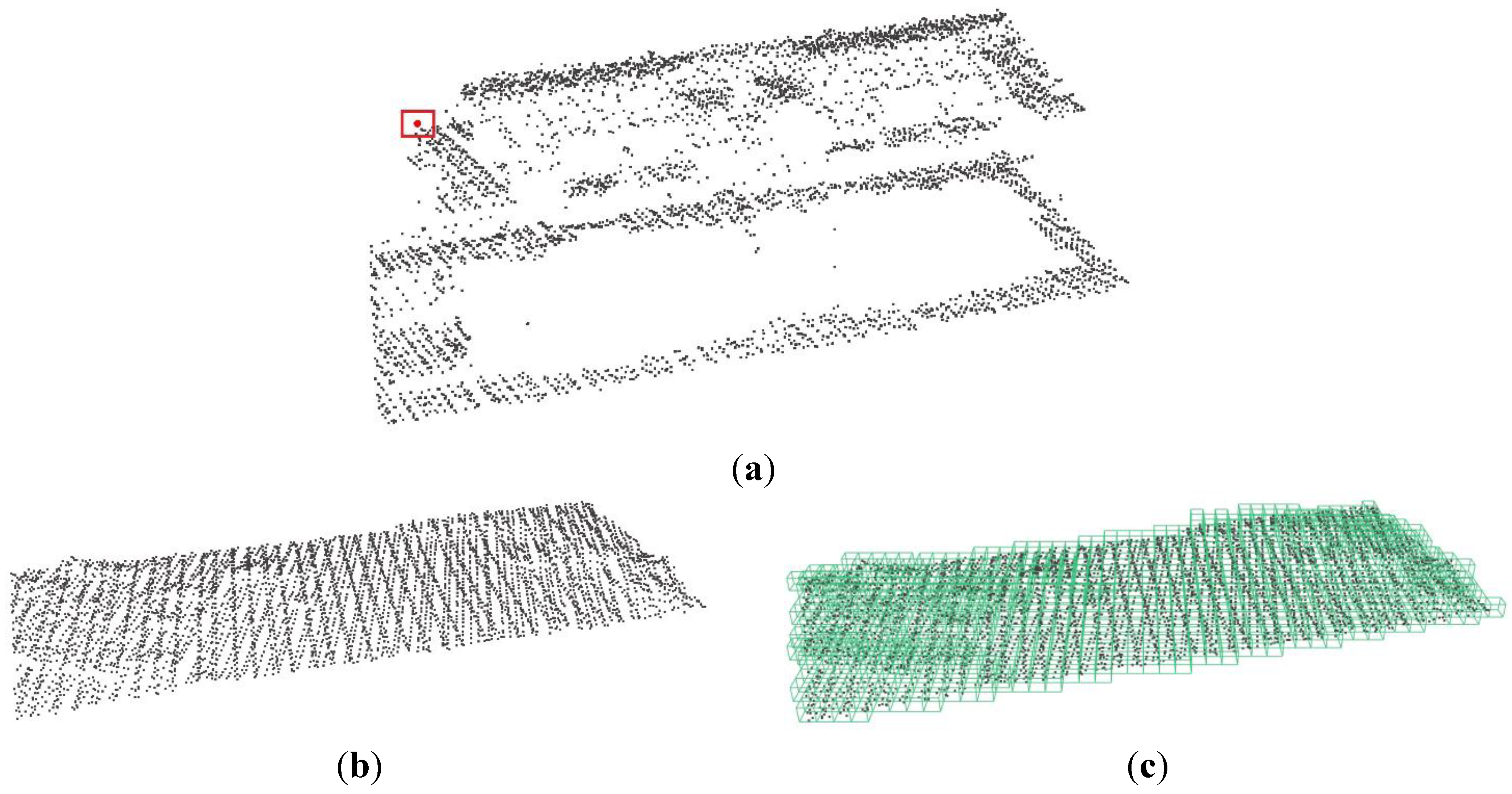
The corresponding leaf node to which the 3D coordinates of point p belong does not exist in the octree index of R₁, i.e., N_p is empty. In this case, p is defined as a changed point. For example, Figure 4a shows LiDAR data for a building at t₂; Figure 4b represents the LiDAR data at t₁ at the same location, and Figure 4c denotes the octree structure for the LiDAR data at t₁. A comparison of the two data sets indicates that there is a newly built building. In the change detection process, the 3D coordinates of point p (red point in the red rectangle in Figure 4a) are input to R₁. As there are no corresponding leaf node containing this 3D coordinates in R₁, the LiDAR points in the leaf node and sibling nodes do not exist, so N_p1 is empty. Such a point p is classified as a changed point.

Figure 4. Example of calculating changed areas. (a) The airborne LiDAR point cloud for a building at t₂; (b) The airborne LiDAR point cloud at t₁ at the same location; (c) The constructed octree for (b).

Figure 4. Example of calculating changed areas. (a) The airborne LiDAR point cloud for a building at t₂; (b) The airborne LiDAR point cloud at t₁ at the same location; (c) The constructed octree for (b).

(2)

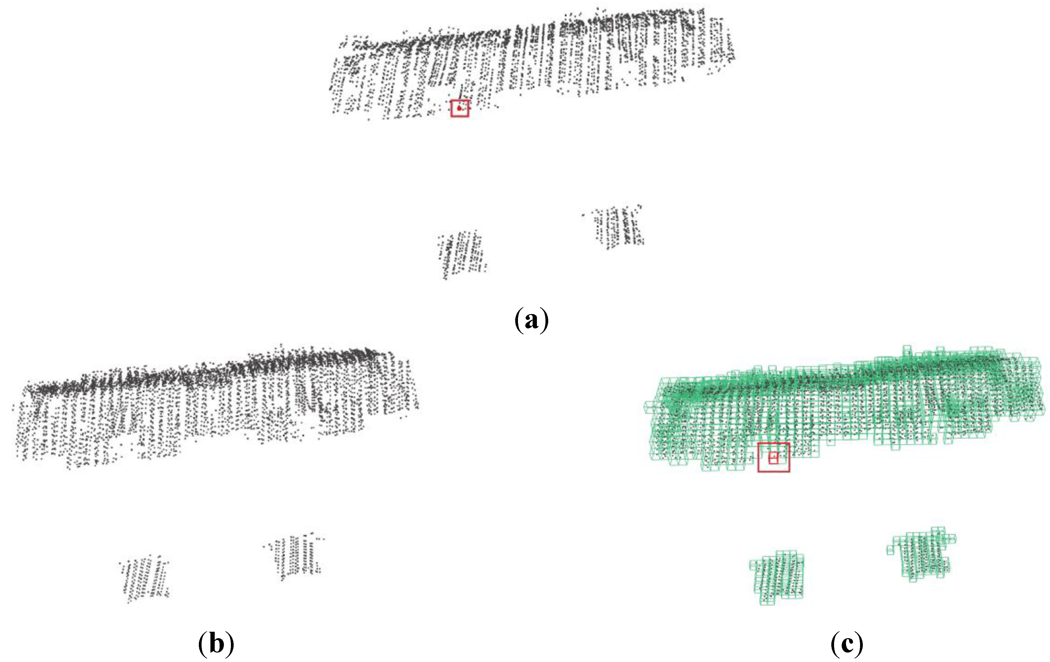
The corresponding leaf node to which the 3D coordinates of point p belong exists in the octree index of R₁, i.e., N_p is not empty. In this case, p is regarded as an unchanged point. For example, Figure 5a shows LiDAR data for a building at t₂; Figure 5b represents the LiDAR data at t₁ at the same location, and Figure 5c denotes the octree structure for the LiDAR data at t₁. The area has not changed from t₁ to t₂. When the 3D coordinates of point p (red point in the red rectangle in Figure 5a) are imported to R₁, the corresponding leaf node containing the 3D coordinates already exist in R₁ (red cube in the red rectangle in Figure 5c). Namely, the LiDAR points in the leaf node and sibling nodes exist in the octree structure of R₁. Therefore, N_p is not empty. When there are some points within a radius r, it indicates that the point p is an unchanged point. Such points are rejected from the change detection results. When there are no points within a radius r, p is defined as a changed point.

Figure 5. Example of unchanged areas. (a) The airborne LiDAR point cloud for a building at t₂; (b) The airborne LiDAR point cloud at t₁ at the same location; (c) The constructed octree for (b).

Figure 5. Example of unchanged areas. (a) The airborne LiDAR point cloud for a building at t₂; (b) The airborne LiDAR point cloud at t₁ at the same location; (c) The constructed octree for (b).

2.3.2. Separation of Buildings and Trees

After obtaining the changed LiDAR point cloud, further processing is required to determine the changed areas of buildings and trees. The changed areas obtained from the octree fully retain the original geometric precision of the airborne LiDAR data, and there is no offset at any location. However, the change detection results contain a certain number of noise points, and the buildings and trees are mixed. Noise points are generally discrete and discontinuous. Thus, we introduce a clustering method to eliminate noise points and separate the buildings from the trees using a classification method. The AutoClust [41] algorithm is selected to perform point cloud clustering, which is based on Delaunay triangulation. We use the fact that the side lengths of the Delaunay triangles are shorter in dense point clouds and longer in sparser areas. The most important point is that the side lengths vary between regions of different density. The triangulation is divided based on the characteristics, so as to realize the clustering of the LiDAR point cloud. The clustering process forms different clusters, each representing a dense point cloud. There will be far fewer points in clusters formed by noise points, and so noise can be eliminated by setting a threshold for the number of points in the clusters. After the noise points have been removed, we can identify the changed buildings and trees. These are then separated according to roughness of points, area, and the average height of the clusters as follows: (1) Use an area threshold to extract large buildings; (2) Employ a height threshold to obtain buildings not detected in step (1); and (3) Apply a roughness threshold to divide low buildings from trees. The classification rules are shown in Figure 6. First, we define the concept of roughness. For point p, by taking it as a center, a sphere with a radius r (1 m in this paper) is created. All points belonging to this sphere are collected and the standard deviation of their height values is calculated, which is used as the roughness value of point p. When the roughness value is smaller than the set threshold, point p is regarded as a building point.

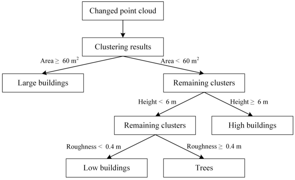
Figure 6. The rules used for separation of buildings and trees.

Figure 6. The rules used for separation of buildings and trees.

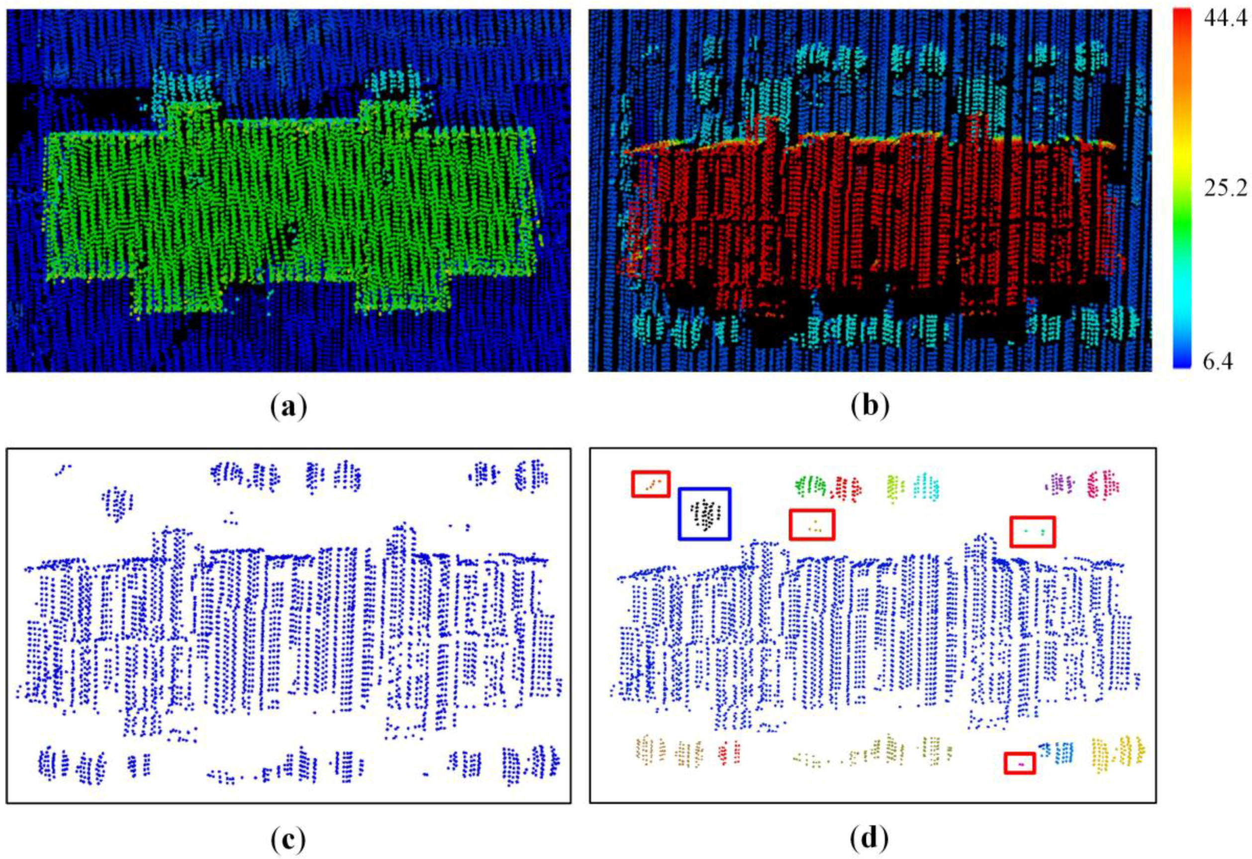
Figure 7a,b shows airborne LiDAR point clouds obtained on different dates from the same location. The comparison of these LiDAR data indicates that there is a change in the building elevation, meaning that the building was built or extended in the period from t₁ to t₂. Figure 7c shows the changed airborne LiDAR points, which include a building, trees, and noise. Figure 7d reveals the clustering results using AutoClust, where different colors represent different clusters. There are fewer points in the clusters in the red rectangles in Figure 7d, which can be regarded as noise, and the blue rectangle in Figure 7d contains more black points. Therefore, the noise points can be removed by setting a threshold for the point number of each cluster. Based on the classification steps introduced in the above paragraph, the new or changed buildings and new trees are identified. To judge whether a detected building is new or changed, it is compared with the earlier LiDAR data, which only include non-ground points. The detected building points and the earlier LiDAR data are put together, and a bounding box (the length of the box should be as long as possible in the z direction) can be defined according to the minimum and maximum x, y coordinates of the detected building points in the 3D space. Then, if there are a number of points (the minimal number of points is set to 100) from the earlier LiDAR data in the bounding box, the detected building is regarded as a changed building; otherwise, it is considered to be a new building.

To identify demolished buildings and felled trees, the octree is constructed from the LiDAR data obtained at later date, as mentioned in Section 2.3. The 3D point coordinates from the earlier date are input to the constructed octree, and the above steps are repeated.

Figure 7. The clustering results of LiDAR points. (a) The airborne LiDAR data at t₁; (b) The airborne LiDAR data at t₂; (c) Changed areas between t₁ and t₂; (d) Clustering results based on (c), where the points in the red rectangle and blue rectangle represent noise and non-noise, respectively.

Figure 7. The clustering results of LiDAR points. (a) The airborne LiDAR data at t₁; (b) The airborne LiDAR data at t₂; (c) Changed areas between t₁ and t₂; (d) Clustering results based on (c), where the points in the red rectangle and blue rectangle represent noise and non-noise, respectively.

3. Study Area and Data

We took Jianye District, Nanjing, in the Jiangsu Province of China, as the study area (Figure 8). The experimental region is generally flat, covering an area of about 2.5 km × 1.5 km. The airborne LiDAR point clouds were collected by an airborne Optech ALTM Gemini laser scanning system from a flying altitude of about 1000 m. The two sets of LiDAR data were obtained on 17 July 2006 and 13 April 2009, and have average point densities of 5.04 pts/m² and 4.51 pts/m², respectively. The aerial orthophotos were taken while collecting the LiDAR data, and are used here to evaluate the experimental results. Figure 8a–d shows the aerial imagery at 0.3 m resolution and the airborne LiDAR data from 2006 and 2009, respectively.

The experimental region is a typical metropolitan area, containing a number of modern high-rise architectures. The second summer youth Olympic Games was held in Nanjing in 2014. Thus, a large number of stadiums and infrastructure, including commercial and residential buildings, were built prior to this event. Comparing Figure 8a,c, vast buildings appear in the northwest and southeast, so the area is ideal for change detection. The largest building in the southwest of Figure 8a,c is the Nanjing Olympic Sports Center, which was the main venue of the 2014 youth Olympics.

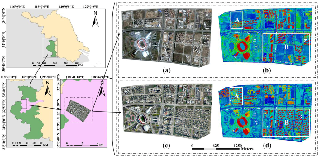
Figure 8. Experimental area. (a) Reference orthoimage for the year 2006; (b) LiDAR data for the year 2006; (c) Reference orthoimage for the year 2009; (d) LiDAR data for the year 2009.

Figure 8. Experimental area. (a) Reference orthoimage for the year 2006; (b) LiDAR data for the year 2006; (c) Reference orthoimage for the year 2009; (d) LiDAR data for the year 2009.

4. Results and Analysis

The proposed method was programmed in C++ and tested on the Microsoft Visual Studio platform (Microsoft Corporation, Redmond, Washington, USA) using a PC with 4 GB of RAM.

4.1. Experimental Results

First, to verify that the proposed method is not limited by the scale of different objects, it was compared with the DSM-based method in a small area. For the DSM-based method, the DSM and digital terrain model (DTM) of two different dates are interpolated from all LiDAR points (ground points and non-ground points) and ground points using the nearest-neighbor interpolation algorithm based on their height values, respectively. The normalized DSM (nDSM) of both dates can be derived according to the difference between DSM and DTM. Meanwhile, the nDSM of the later date is subtracted from that of the earlier date to obtain delta DSM (dDSM). Then, the intersection of nDSM and dDSM is used to detect and locate the final changed areas. The method is described in detail in the literature [23]. On account of our approach being a point-based method, it was also compared with a voxel-based method to test its efficiency. For these two point-based methods, all steps of change detection are the same, except for the data structure for storing LiDAR points.

These two comparative experiments were conducted in partial experimental regions (Regions A and B in the white rectangles in Figure 8b,d). All main thresholds of the proposed approach are summarized in Table 2, and these values were used in the subsequent experiments. The minimal node size, search radius, and height are set according to data source (i.e., airborne LiDAR data). The minimal number of points, minimal number of points in a cluster, and roughness are set empirically. The small area is set according to the situation of the study area.

Table 2. The key thresholds of the proposed approach.

No	Items	Thresholds	Description	Setting Basis
1	Minimal node size	2 m	To terminate an octant subdivided into eight octants.	Data source
2	Minimal number of points	2 pts	Minimal number of points contained in a node.	Empiric
3	Search radius	1 m	If Np is not empty, the points in the radius of r are searched.	Empiric
4	Minimal number of points in a cluster	5 pts	To remove noise points in the changed areas.	Empiric
5	Small area	60 m2	To detect the large buildings from the changed areas.	Study area
6	Height	6 m	To extract the high buildings from the changed areas.	Study area
7	Roughness	0.4 m	To separate the trees from the low buildings.	Empiric

Table 2. The key thresholds of the proposed approach.

No	Items	Thresholds	Description	Setting Basis
1	Minimal node size	2 m	To terminate an octant subdivided into eight octants.	Data source
2	Minimal number of points	2 pts	Minimal number of points contained in a node.	Empiric
3	Search radius	1 m	If Np is not empty, the points in the radius of r are searched.	Empiric
4	Minimal number of points in a cluster	5 pts	To remove noise points in the changed areas.	Empiric
5	Small area	60 m2	To detect the large buildings from the changed areas.	Study area
6	Height	6 m	To extract the high buildings from the changed areas.	Study area
7	Roughness	0.4 m	To separate the trees from the low buildings.	Empiric

Figure 9a,b shows the airborne LiDAR data from Region A (white rectangles in Figure 8b,d) for 2006 and 2009, respectively. Figure 9c reveals the change detection results given by the proposed approach. The output is in the form of a point cloud, and Figure 9d represents the rasterized results of the point cloud in Figure 9c, where the grid cell size is 1 m. The white areas denote changed areas containing new buildings and new trees, and black areas denote unchanged areas. Figure 9e shows the result generated by the DSM-based method, which eliminates the unchanged areas. However, Figure 9e still contains a lot of noise. To obtain a better result, a morphological filtering algorithm with a small window size of 3 m × 3 m, which could reserve more detailed information about changed objects, was used to remove the noise. Figure 9f shows the final results of the DSM-based method. The pixel size of the DSM is set to 1 m, which is determined according to the point spacing of LiDAR point clouds. In the study of Yan et al. [42], they suggest that most of the previous studies used 0.5 m to 1 m data resolution, which seems to be a good trade-off between the mean point spacing and point density. In addition, there was ongoing construction in the study area used in this paper, where the trees are small. If the pixel size of the DSM is set to 0.5 m, there may be some errors in the interpolation result since fewer LiDAR points exist in one pixel, and as the pixels representing the trees are still small, could be removed when using a morphological filtering algorithm. We find that there are only new buildings and new trees in Region A according to the revelation of aerial images. We compared the change detection results of the proposed method and the DSM-based method with the real changed areas, which were extracted manually from the aerial images and airborne LiDAR data from two dates. In Region A, there are 19 new buildings, which are detected accurately both by the proposed method and the DSM-based method. Table 3 lists the comparative results of these two methods detecting new trees. An extracted area of 5885.29 m² is obtained by the proposed method, whereas an area of 473.56 m² is omitted. However, the DSM-based method only has an extracted area of 32.57 m² and a large number of new trees are not detected. Therefore, a comparison of the two methods’ results indicates that the proposed method handles the change detection of trees significantly better than the DSM-based method. It can be concluded that the proposed method is not affected by the scales of different objects.

Figure 9. Comparison between the proposed approach and the DSM-based method. (a) LiDAR data for the year 2006; (b) LiDAR data for the year 2009; (c) Output of the proposed approach; (d) Rasterized results of (c); (e) Output of the DSM-based method; (f) Final results of the DSM-based method after the use of a morphological filter with 3 m × 3 m.

Figure 9. Comparison between the proposed approach and the DSM-based method. (a) LiDAR data for the year 2006; (b) LiDAR data for the year 2009; (c) Output of the proposed approach; (d) Rasterized results of (c); (e) Output of the DSM-based method; (f) Final results of the DSM-based method after the use of a morphological filter with 3 m × 3 m.

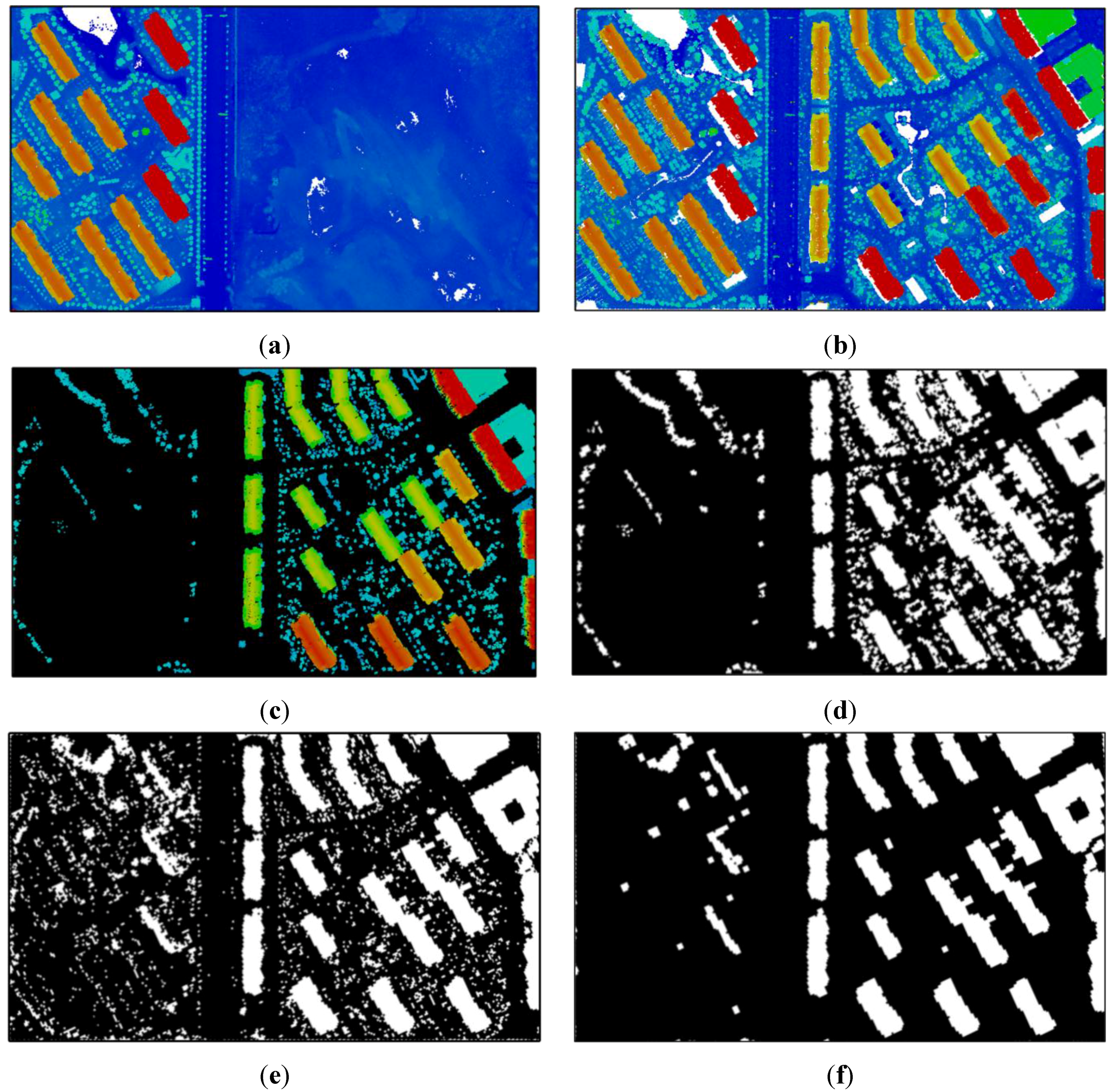
Table 3. Change detection results for new trees of the proposed method and the DSM-based method in Region A.

Methods	Categories	Extracted Area (m2)	Omissive Area (m2)	Total Area (m2)
Octree-based method	New trees	5885.29	473.56	6358.85
DSM-based method		32.57	6326.28

Table 3. Change detection results for new trees of the proposed method and the DSM-based method in Region A.

Methods	Categories	Extracted Area (m2)	Omissive Area (m2)	Total Area (m2)
Octree-based method	New trees	5885.29	473.56	6358.85
DSM-based method		32.57	6326.28

Table 4 lists the comparative results for Regions A and B (white rectangles in Figure 8b,d) between the proposed method and the voxel-based method, where the voxel size was set to 2 m. Although the execution time of the voxel-based method is less than that of the octree-based method, the proposed method requires significantly less memory. Hence, the voxel-based method is unsuitable for change detection over large areas, as the memory requirements would exceed those available in a mainstream computer. For example, when the voxel-based method was implemented on the whole experimental region, we encountered an out-of-memory error.

Table 4. Execution times and memory requirements for the octree- and voxel-based methods.

Regions	Methods	Number of Points		Time (s)	Size in Memory
		2006	2009
Region A	Octree-based method	563,187	563,050	62.15	26.12 MB
	Voxel-based method			58.12	173.86 MB
Region B	Octree-based method	4,317,880	3,346,283	883.69	152.45 MB
	Voxel-based method			735.67	4146.91 MB
Whole Region	Octree-based method	20,569,302	17,381,481	5365.09	727.59 MB
	Voxel-based method			Failed	Failed

Table 4. Execution times and memory requirements for the octree- and voxel-based methods.

Regions	Methods	Number of Points		Time (s)	Size in Memory
		2006	2009
Region A	Octree-based method	563,187	563,050	62.15	26.12 MB
	Voxel-based method			58.12	173.86 MB
Region B	Octree-based method	4,317,880	3,346,283	883.69	152.45 MB
	Voxel-based method			735.67	4146.91 MB
Whole Region	Octree-based method	20,569,302	17,381,481	5365.09	727.59 MB
	Voxel-based method			Failed	Failed

Figure 10. Change detection results for the entire experimental area.

Figure 10. Change detection results for the entire experimental area.

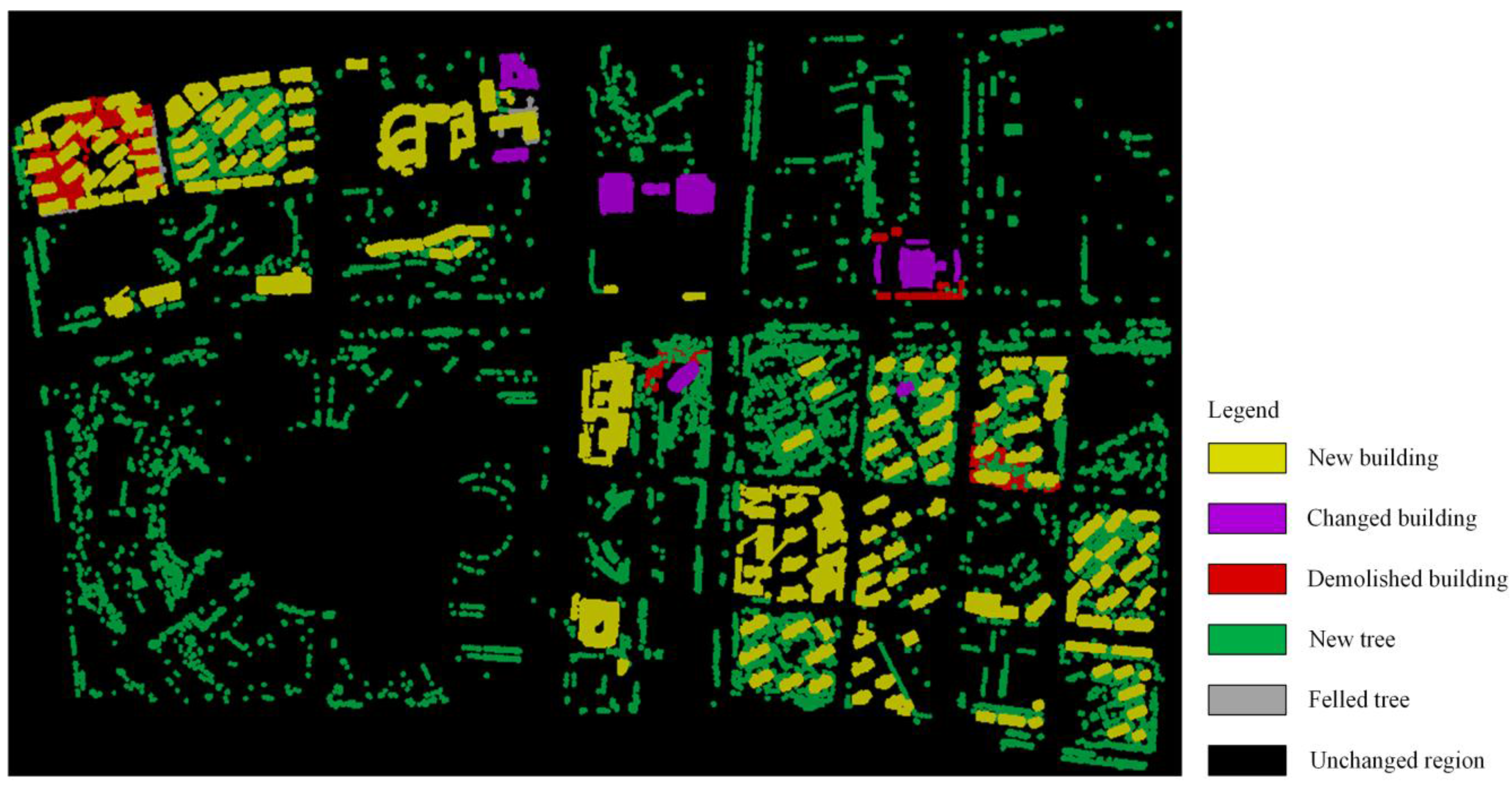
Figure 10 shows the results given by the proposed approach when applied to the entire experimental region. Yellow, violet, red, green, gray, and black denotes new buildings, changed buildings, demolished buildings, new trees, felled trees, and unchanged regions, respectively. Each type of change is highlighted in Figure 11.

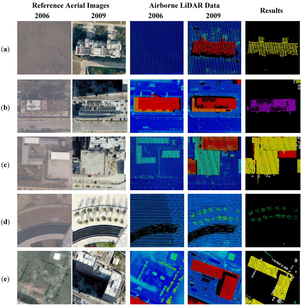
Figure 11. Example of the five change types. (a) New building; (b) Changed building; (c) Demolished buildings; (d) New trees; (e) Felled trees.

Figure 11. Example of the five change types. (a) New building; (b) Changed building; (c) Demolished buildings; (d) New trees; (e) Felled trees.

4.2. Experimental Analysis

To evaluate the effectiveness of the proposed approach for detecting changes in buildings and trees, a comparative analysis between the change detection results and the reference data was conducted. The reference data was obtained from a visual interpretation of the aerial images and airborne LiDAR data from two dates. The experimental results and the reference data are put together: (1) overlain regions, in which the ratio of the overlapping area is more than 60%, taken as correct detection; (2) regions only existing in the reference data taken as misdetection; and (3) regions only existing in the detected regions, or overlain regions whose ratios of the overlapping areas are less than 20%, taken as wrong detection. Aforementioned, three situations are determined visually. Since individual plant separation is not achieved by the proposed method, there may be a condition whereby multiple trees belong to a cluster. In this case, the evaluation for buildings and trees will be based on the quantity and the area, respectively. Therefore, three parameters were measured to evaluate the experimental results as follows:

$$Completeness=\frac{TP}{TP+FN}$$

(1)

$$Correctness=\frac{TP}{TP+FP}$$

(2)

$$Quality=\frac{TP}{TP+FP+FN}$$

(3)

where TP (true positive) represents the quantity or area of correct detections; FN (false negative) represents the quantity or area of misdetections; and FP (false positive) represents the quantity or area of wrong detections.

Table 5 shows the confusion matrix obtained from this comparison between the experimental results of buildings and the reference data. It provides information on the percentage of changed regions that were detected (completeness) or correct (correctness). For new buildings, the completeness and correctness are 100.00% and 97.56%, respectively. Since the proposed approach is a point-based method, comparing the point similarity enables the point cloud representing newly built buildings to be found. This part of the point cloud does not exist in the LiDAR data from 2006. Therefore, the completeness of the new buildings is 100.00%. The completeness and correctness are 91.18% and 100.00% for demolished buildings, respectively. There are 12 buildings that were misclassified as “other”. Here, other mainly refers to the ground. The main causes of misclassification are demolished buildings having a low height or parts of buildings being sheltered, resulting in 12 buildings assigned as ground points during the separation process. The completeness and correctness of changed buildings are 80.00% and 100.00%, respectively. Two changed buildings were misclassified as new buildings. This is mainly because the height of the changed buildings is so low in 2006 that the buildings were classified as ground points. Therefore, the point clouds representing these changed buildings do not exist as non-ground points. Hence, these buildings can only be judged as new buildings. From Table 5, we can draw a number of conclusions: (1) The overall accuracy of the proposed approach for the change detection of buildings can reach 94.81%; (2) There is no misclassification between new buildings and demolished buildings; (3) In the experimental area, the change types of buildings are mainly new buildings and demolished buildings. Referring to the aerial images, new buildings and demolished buildings are mostly residential buildings and building site sheds, respectively.

Table 6 shows the evaluation results for the change detection of trees. The completeness, correctness, and quality of new trees are 91.90%, 88.93%, and 82.38%, respectively. The results suggest that an area of 8963.46 m² was incorrectly classified as new trees. The reason for this error is that we only extracted areas of newly planted trees, and rejected the changed areas caused by the natural growth of trees in the process of obtaining reference data. However, the change detection results include areas that have changed because of the natural growth of trees. This phenomenon cannot be avoided using a point-based method. Although the change in tree cover is small over a relatively short period, it caused some errors in the final results. An area of 6284.61 m² of new trees was not classified as such by our method. These trees are mainly close to buildings, and so the occlusion of the buildings caused these trees to not be collected by the airborne laser scanner. In addition, some newly planted trees are so small that they were not extracted. The completeness, correctness, and quality of felled trees detection are 96.64%, 87.81%, and 85.22%, respectively. False positives of the felled trees covered an area of 216.76 m², and were mainly because of changes in other types of surface feature. False negatives of the felled trees covered just 54.37 m², which is within an acceptable error range over this large area.

Table 5. Confusion matrix for the change detection results of buildings.

	Reference Data
Change Detection Results	New Buildings	Demolished Buildings	Changed Buildings	Other	Row Total	Correctness (%)
New Buildings	160	0	2	2	164	97.56
Demolished Buildings	0	124	0	0	124	100.00
Changed Buildings	0	0	8	0	8	100.00
Other	0	12	0	-	12	-
Column Total	160	136	10	2	308	-
Completeness (%)	100.00	91.18	80.00	100.00	-	94.81

Table 5. Confusion matrix for the change detection results of buildings.

	Reference Data
Change Detection Results	New Buildings	Demolished Buildings	Changed Buildings	Other	Row Total	Correctness (%)
New Buildings	160	0	2	2	164	97.56
Demolished Buildings	0	124	0	0	124	100.00
Changed Buildings	0	0	8	0	8	100.00
Other	0	12	0	-	12	-
Column Total	160	136	10	2	308	-
Completeness (%)	100.00	91.18	80.00	100.00	-	94.81

Table 6. Evaluation of the change detection results for trees.

Categories	TP (m2)	FP (m2)	FN (m2)	Completeness (%)	Correctness (%)	Quality (%)
New Trees	71,307.18	8963.46	6284.61	91.90	88.83	82.38
Felled Trees	1562.83	216.76	54.37	96.64	87.81	85.22

Table 6. Evaluation of the change detection results for trees.

Categories	TP (m2)	FP (m2)	FN (m2)	Completeness (%)	Correctness (%)	Quality (%)
New Trees	71,307.18	8963.46	6284.61	91.90	88.83	82.38
Felled Trees	1562.83	216.76	54.37	96.64	87.81	85.22

An analysis of the results in Table 5 and Table 6 suggests that the difficulty of detecting changes in trees is significantly greater than that for buildings. Based on this, we varied the search radius and the roughness parameters to examine the impact of these thresholds on the experimental results for new trees. Figure 12a shows the accuracy of different search radiuses for the change detection of new trees. As the search radius increases, the correctness rises, but the completeness falls. The reason for this reduction in completeness is that the newly planted trees are close to buildings. The newly planted trees only exist in the point cloud from the later date. When the 3D coordinates of these tree points are input to the point cloud from the earlier date, those building points close to these 3D coordinates are mistaken for tree points resulting in that the newly planted trees are considered to have existed in the earlier point cloud. In other words, there is no change here. The correctness increases because the redundant portion caused by the natural growth of trees is lower. As can be seen from Figure 12a, a search radius of between 1.0 m and 1.2 m is optimal. Therefore, we select 1 m as the threshold for the search radius. Figure 12b represents the effects of different roughness values on the change detection accuracy of newly planted trees. With an increase in roughness, the completeness decreases, although the correctness remains almost unchanged. The completeness continues to decrease because some newly planted trees with lower roughness are not detected.

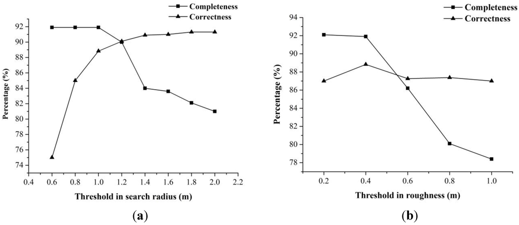
Figure 12. Accuracy estimates for the change detection results of new trees. (a) Effect of changing the search radius; (b) Effect of changing the roughness.

Figure 12. Accuracy estimates for the change detection results of new trees. (a) Effect of changing the search radius; (b) Effect of changing the roughness.

5. Discussion

The detection results in Figure 10 and the evaluation outcomes in Table 5 and Table 6 demonstrate the good performance of the proposed method in an urban area. At present, the use of airborne LiDAR data to detect changes in urban environments is mostly based on DSMs. This paper has compared the proposed approach with the DSM-based method over a small experimental area. The pixel size of the DSM and the window size of the morphological filtering algorithm are set to 1 m, and 3 m × 3 m by trial and error, respectively. In other words, these parameter settings are optimal for the DSM-based method. The experimental results show that the proposed approach has the same accuracy as the DSM-based method for detecting changes to buildings. However, the proposed approach is significantly better than the DSM-based method for detecting changes in tree cover. The DSM-based method converts the LiDAR points into raster data. In this case, there are few grid cells representing trees. Changed areas are detected by subtracting the DSMs from the two datasets and applying the morphological filtering algorithm. However, in this step, the changed areas of trees can easily be removed. The proposed approach determines the changed areas by directly comparing the different LiDAR point clouds. Thus, the accuracy of the experimental results is ensured by avoiding the rasterization step, which can easily produce intermediate errors.

Although the proposed approach obtained good results for the change detection of trees, there were some misclassification phenomena, especially where the natural growth of trees was misclassified as new trees. This problem cannot be solved under the condition of only having airborne LiDAR, because the sparse airborne LiDAR point clouds from two dates differ to a certain extent in terms of point density, and the spatial relationship between different objects is difficult to determine according to the discrete points. In addition, there was ongoing construction in the study area from 2006 to 2009. Therefore, the sizes of the new trees and the natural growth of trees are both small. This leads to the fact that the point-based method is difficult to separate them from each other. This problem can be solved by introducing the ancillary data, e.g., the existing vector map. For example, if we have the land cover map of 2006, we can confirm the locations of the existing trees. The changed points around these trees could be considered to belong to the natural growth of trees.

The registration of two point clouds is vital for the point-based method. If there is a registration offset of 1–2 m, it would be difficult to detect changes in tree cover. The proposed method uses the ICP algorithm to accurately register the LiDAR point clouds. Experimental results show that the ICP algorithm can meet the registration accuracy requirement. In general, the ICP algorithm has sufficient stability and robustness for the registration of different point clouds. However, it requires an accurate initial state to ensure global convergence. Therefore, before using the ICP algorithm for data registration, we must somehow guarantee that the two point clouds have a good initial state. The point density is also important for change detection of trees. If the point density is small, few points will represent a single tree. These points may be mistaken for noise and removed. The experimental data used in this study have a point density of 5 pts/m², and the results show that this is sufficient to allow change detection in trees to some extent.

6. Conclusions

This paper has presented a new point-based approach based on octrees using airborne LiDAR data for the automatic detection of changed areas of buildings and trees. The main contributions of the proposed approach are summarized as follows: (1) The proposed approach establish a complete set of processes to detect changes in buildings and trees to urban areas; (2) The proposed point-based approach is well suited to change detection in multiple targets, as it is not affected by the scales of different objects. The introduction of this octree structure allows the LiDAR points to be indexed efficiently, so as not to consume too much memory, and guarantees the accuracy of the change detection results. The experimental results show that the proposed method detects change in buildings and trees well. The type of change to the buildings and trees was also effectively determined. The overall accuracy for change detection of buildings and trees reached 94.8% and 83.8%, respectively. Therefore, the proposed approach can be used as an alternative method for detecting changes in buildings and trees in urban areas.

In future work, we intend to improve the change detection in areas of trees, because changed areas caused by the natural growth of trees were regarded as areas of new trees in this study. This caused a degree of misclassification between newly planted trees and existing trees that had simply grown. The proposed approach will be applied to different experimental areas to further test its scientific validity and effectiveness. In an urban environment there are other types of feature change. Future work will combine multiple sources to detect changes in all features of the urban environment.

References

- Tian, J.J.; Cui, S.Y.; Reinartz, P. Building change detection based on satellite stereo imagery and digital surface models. IEEE Trans. Geosci. Remote Sens. 2014, 52, 406–417. [Google Scholar] [CrossRef]
- Knudsen, T.; Olsen, B.P. Automated change detection for updates of digital map databases. Photogramm. Eng. Remote Sens. 2003, 69, 1289–1296. [Google Scholar] [CrossRef]
- Nebiker, S.; Lack, N.; Deuber, M. Building change detection from historical aerial photographs using dense image matching and object-based image analysis. Remote Sens. 2014, 6, 8310–8336. [Google Scholar] [CrossRef]
- Im, J.; Jensen, J.R.; Tullis, J.A. Object-based change detection using correlation image analysis and image segmentation. Int. J. Remote Sens. 2008, 29, 399–423. [Google Scholar] [CrossRef]
- Hussain, M.; Chen, D.M.; Cheng, A.; Wei, H.; Stanley, D. Change detection from remotely sensed images: From pixel-based to object-based approaches. ISPRS J. Photogramm. Remote Sens. 2013, 80, 91–106. [Google Scholar] [CrossRef]
- Jung, F. Detecting building changes from multitemporal aerial stereopairs. ISPRS J. Photogramm. Remote Sens. 2004, 58, 187–201. [Google Scholar] [CrossRef]
- Stal, C.; Tack, F.; de Maeyer, P.; de Wulf, A.; Goossens, R. Airborne photogrammetry and LiDAR for DSM extraction and 3D change detection over an urban area—A comparative study. Int. J. Remote Sens. 2013, 34, 1087–1110. [Google Scholar] [CrossRef]
- Walter, V. Object-based classification of remote sensing data for change detection. ISPRS J. Photogramm. Remote Sens. 2004, 58, 225–238. [Google Scholar] [CrossRef]
- Liu, X.L.; Bo, Y.C. Object-based crop species classification based on the combination of airborne hyperspectral images and LiDAR data. Remote Sens. 2015, 7, 922–950. [Google Scholar] [CrossRef]
- Antonarakis, A.S.; Richards, K.S.; Brasington, J. Object-based land cover classification using airborne LiDAR. Remote Sens. Environ. 2008, 112, 2988–2998. [Google Scholar] [CrossRef]
- Kankare, V.; Raty, M.; Yu, X.W.; Holopainen, M.; Vastaranta, M.; Kantola, T.; Hyyppä, J.; Hyyppä, H.; Alho, P.; Viitala, R. Single tree biomass modelling using airborne laser scanning. ISPRS J. Photogramm. Remote Sens. 2013, 85, 66–73. [Google Scholar] [CrossRef]
- Cheng, L.; Wu, Y.; Wang, Y.; Zhong, L.; Chen, Y.; Li, M. Three-dimensional reconstruction of large multilayer interchange bridge using airborne LiDAR data. IEEE J. Sel. Top. Appl. Earth Observ. Remote Sens. 2015, 8, 691–707. [Google Scholar] [CrossRef]
- Matikainen, L.; Hyyppä, J.; Ahokas, E.; Markelin, L.; Kaartinen, H. Automatic detection of buildings and changes in buildings for updating of maps. Remote Sens. 2010, 2, 1217–1248. [Google Scholar] [CrossRef]
- Tian, J.; Reinartz, P.; d’Angelo, P.; Ehlers, M. Region-based automatic building and forest change detection on Cartosat-1 stereo imagery. ISPRS J. Photogramm. Remote Sens. 2013, 79, 226–239. [Google Scholar] [CrossRef]
- Chen, L.C.; Lin, L.J. Detection of building changes from aerial images and light detection and ranging (LiDAR) data. J. Appl. Remote Sens. 2010, 4. [Google Scholar] [CrossRef]
- Matikainen, L.; Hyyppä, J.; Kaartinen, H. Automatic detection of changes from laser scanner and aerial image data for updating building maps. Int. Arch. Photogramm. Remote Sens. Spat. Inf. Sci. 2004, 35, 434–439. [Google Scholar]
- Vosselman, G.; Gorte, B.; Sithole, G. Change detection for updating medium scale maps using laser altimetry. Int. Arch. Photogramm. Remote Sens. Spat. Inf. Sci. 2004, 35, 207–212. [Google Scholar]
- Malpica, J.A.; Alonso, M.C.; Papí, F.; Arozarena, A.; Martínez de Agirre, A. Change detection of buildings from satellite imagery and LiDAR data. Int. J. Remote Sens. 2013, 34, 1652–1675. [Google Scholar] [CrossRef]
- Wang, Y.; Ziedins, I.; Holmes, M.; Challands, N. Tree models for difference and change detection in a complex environment. Ann. Appl. Stat. 2012, 6, 1162–1184. [Google Scholar] [CrossRef]
- Kaasalainen, S.; Krooks, A.; Liski, J.; Raumonen, P.; Kaartinen, H.; Kaasalainen, M.; Puttonen, E.; Anttila, K.; Makipaa, R. Change detection of tree biomass with terrestrial laser scanning and quantitative structure modelling. Remote Sens. 2014, 6, 3906–3922. [Google Scholar] [CrossRef]
- Murakami, H.; Nakagawa, K.; Hasegawa, H.; Shibata, T.; Iwanami, E. Change detection of buildings using an airborne laser scanner. ISPRS J. Photogramm. Remote Sens. 1999, 54, 148–152. [Google Scholar] [CrossRef]
- Vu, T.T.; Matsuoka, M.; Yamazaki, F. LiDAR-based change detection of buildings in dense urban areas. IEEE Int. Geosci. Remote Sens. Symp. 2004, 5, 3413–3416. [Google Scholar]
- Teo, T.A.; Shih, T.Y. LiDAR-based change detection and change-type determination in urban areas. Int. J. Remote Sens. 2013, 34, 968–981. [Google Scholar] [CrossRef]
- Pang, S.Y.; Hu, X.Y.; Wang, Z.Z.; Lu, Y.H. Object-based analysis of airborne LiDAR data for building change detection. Remote Sens. 2014, 6, 10733–10749. [Google Scholar] [CrossRef]
- Zhang, X.; Glennie, C. Change detection from differential airborne LiDAR using a weighted anisotropic iterative closest point algorithm. IEEE Int. Geosci. Remote Sens. Symp. 2014. [Google Scholar] [CrossRef]
- Girardeau-Montaut, D.; Roux, M.; Marc, R.; Thibault, G. Change detection on points cloud data acquired with a ground laser scanner. Int. Arch. Photogramm. Remote Sens. Spat. Inf. Sci. 2005, 36, W19. [Google Scholar]
- Richter, R.; Kyprianidis, J.E.; Döllner, J. Out-of-core GPU-based change detection in massive 3D point clouds. Trans. GIS 2013, 17, 724–741. [Google Scholar] [CrossRef]
- Barber, D.; Holland, D.; Mills, J. Change detection for topographic mapping using three-dimensional data structures. Int. Arch. Photogramm. Remote Sens. Spat. Inf. Sci. 2008, 37, 1177–1182. [Google Scholar]
- Houldcroft, C.J.; Campbell, C.L.; Davenport, I.J.; Gurney, R.J.; Holden, N. Measurement of canopy geometry characteristics using LiDAR laser altimetry: A feasibility study. IEEE Trans. Geosci. Remote Sens. 2005, 43, 2270–2282. [Google Scholar]
- Yu, X.W.; Hyyppä, J.; Kaartinen, H.; Maltamo, M. Automatic detection of harvested trees and determination of forest growth using airborne laser scanning. Remote Sens. Environ. 2004, 90, 451–462. [Google Scholar] [CrossRef]
- Yu, X.W.; Hyyppä, J.; Kukko, A.; Maltamo, M.; Kaartinen, H. Change detection techniques for canopy height growth measurements using airborne laser scanner data. Photogramm. Eng. Remote Sens. 2006, 72, 1339–1348. [Google Scholar] [CrossRef]
- Meng, X.L.; Currit, N.; Zhao, K.G. Ground filtering algorithms for airborne LiDAR data: A review of critical issues. Remote Sens. 2010, 2, 833–860. [Google Scholar] [CrossRef]
- Gressin, A.; Mallet, C.; Demantke, J.; David, N. Towards 3D LiDAR point cloud registration improvement using optimal neighborhood knowledge. ISPRS J. Photogramm. Remote Sens. 2013, 79, 240–251. [Google Scholar] [CrossRef]
- Cheng, L.; Tong, L.; Li, M.; Liu, Y. Semi-automatic registration of airborne and terrestrial laser scanning data using building corner matching with boundaries as reliability check. Remote Sens. 2013, 5, 6260–6283. [Google Scholar] [CrossRef]
- Bae, K.H.; Lichti, D.D. A method for automated registration of unorganised point clouds. ISPRS J. Photogramm. Remote Sens. 2008, 63, 36–54. [Google Scholar] [CrossRef]
- Besl, P.J.; Mckay, N.D. A method for registration of 3-D shapes. IEEE Trans. Pattern Anal. Mach. Intell. 1992, 14, 239–256. [Google Scholar] [CrossRef]
- Axelsson, P. DEM generation from laser scanner data using adaptive TIN models. Int. Arch. Photogramm. Remote Sens. 2000, 33, 111–118. [Google Scholar]
- Linh, T.H.; Laefer, D.F. Octree-based, automatic building facade generation from LiDAR data. Comput. Aided Des. 2014, 53, 46–61. [Google Scholar]
- Elseberg, J.; Borrmann, D.; Nuchter, A. One billion points in the cloud—An octree for efficient processing of 3D laser scans. ISPRS J. Photogramm. Remote Sens. 2013, 76, 76–88. [Google Scholar] [CrossRef]
- Elsheikh, A.H.; Elsheikh, M. A consistent octree hanging node elimination algorithm for hexahedral mesh generation. Adv. Eng. Softw. 2014, 75, 86–100. [Google Scholar] [CrossRef]
- Estivill-Castro, V.; Lee, I. Argument free clustering for large spatial point-data sets via boundary extraction from delaunay diagram. Comput. Environ. Urban Syst. 2002, 26, 315–334. [Google Scholar] [CrossRef]
- Yan, W.Y.; Shaker, A.; EI-Ashmawy, N. Urban land cover classification using airborne LiDAR data: A review. Remote Sens. Environ. 2015, 158, 295–310. [Google Scholar] [CrossRef]
© 2015 by the authors; licensee MDPI, Basel, Switzerland. This article is an open access article distributed under the terms and conditions of the Creative Commons Attribution license (http://creativecommons.org/licenses/by/4.0/).