Abstract
Three synchronized pulsed Doppler wind lidars were deployed from May 2016 to June 2016 on the shores of a wide Norwegian fjord called Bjørnafjord to study the wind characteristics at the proposed location of a planned bridge. The purpose was to investigate the potential of using lidars to gather information on turbulence characteristics in the middle of a wide fjord. The study includes the analysis of the single-point and two-point statistics of wind turbulence, which are of major interest to estimate dynamic wind loads on structures. The horizontal wind components were measured by the intersecting scanning beams, along a line located 25 above the sea surface, at scanning distances up to 4.6 . For a mean wind velocity above 8 s, the recorded turbulence intensity was below 0.06 on average. Even though the along-beam spatial averaging leads to an underestimated turbulence intensity, such a value indicates a roughness length much lower than provided in the European standard EN 1991-1-4:2005. The normalized spectrum of the along-wind component was compared to the one provided by the Norwegian Petroleum Industry Standard and the Norwegian Handbook for bridge design N400. A good overall agreement was observed for wave-numbers below . The along-beam spatial averaging in the adopted set-up prevented a more detailed comparison at larger wave-numbers, which challenges the study of wind turbulence at scanning distances of several kilometres. The results presented illustrate the need to complement lidar data with point-measurement to reduce the uncertainties linked to the atmospheric stability and the spatial averaging of the lidar probe volume. The measured lateral coherence was associated with a decay coefficient larger than expected for the along-wind component, with a value around 21 for a mean wind velocity bounded between 10 s and 14 s, which may be related to a stable atmospheric stratification.
1. Introduction
As part of a national project to modernize the highway network in Western Norway, the Norwegian Public Roads Administration (NPRA) plans to build a bridge crossing the 5 wide and 550 deep Bjørnafjord, about 30 South of Bergen. For various design concepts, the sensitivity to wind turbulence is a major issue, requiring a detailed analysis of wind turbulence in the fjord.
The application of Doppler wind lidars to study wind field characteristics at scanning distances larger than 1 is quite recent. At the location of the planned crossing, no infrastructure is available to support anemometers. The use of remote sensing technology to complement wind data from sensors on land is, therefore, an attractive option. As presented in Table 1, the mean value and the standard deviation of the wind velocity are the statistics most often studied. To properly estimate wind loading on a wind-sensitive civil engineering structure, the wind velocity spectrum and the wind coherence are in addition required.

Table 1.
Previous field measurements conducted using scanning pulsed lidar(s) to measure wind statistics in the surface layer at scanning distances larger than 1 , such as the mean wind velocity , the velocity standard deviation , the turbulence length scales L, the wind velocity spectrum S and/or the coherence .
There is hardly any study to be found on the turbulence characteristics in the middle of a wide fjord within a coastal area. For example, it is uncertain whether a spectral wind model developed for an offshore or an onshore environment should be used. The present study investigates, therefore, the validity of the wind velocity spectral model provided in the Handbook N400 [9] used for bridge structures in Norway and the model provided by the Norwegian Petroleum Industry Standard [10] for environmental loads on offshore structures, which is more widely known as the NORSOK standard. Only few studies reported in the literature deal with the applicability of lidars to measure wind coherence. The along-beam wind coherence estimated using a single pulsed lidar [11,12,13] is only of limited relevance for estimating wind loading on a long-span bridge, the response of which is governed by the lateral coherence of turbulence. Regarding the lateral coherence of the along-wind component, encouraging results were obtained from pilot lidar measurements using limited data sets [6,14]. The estimation of the lateral coherence of the vertical wind component using synchronized wind lidars is, on the other hand, considerably more challenging because of the need to use relatively large elevation angles to properly observe the vertical wind velocity component. To measure this component, Fuertes et al. [15] used for example an elevation angle of 45°, in a triple-lidar system, whereas Mann et al. [16] used an elevation angle of 34°. In the present study, a triple lidar system is also used. However, the large scanning distances and the associated small elevation angles prevented the measure of the vertical wind component. The three long-range lidars, synchronized in a so-called WindScanner system [17] developed by the Technical University of Denmark (DTU), were deployed in the West sector of the Bjørnafjord from May 2016 to June 2016. The measurement campaign was developed as a research collaboration between the University of Stavanger, Christian Michelsen Research and the Technical University of Denmark (DTU).
Our main objective is to assess whether a system of synchronized long-range Doppler wind lidars can be used to measure the single-point wind spectrum and the wind coherence of the along-wind component, at distances up to 4.6 . The investigation relies, largely, on a comparison with empirical spectral models established since the 1960s to describe wind turbulence, as well as the knowledge gathered from previous measurement campaigns conducted with the long-range WindScanner system. The present paper is, therefore, organized as follows: firstly, the deployment location of the three lidars is presented as well as their scanning configurations. Secondly, a preliminary analysis of the single-point wind turbulence statistics is given. Thirdly, the along-wind turbulence spectrum is compared to the one provided by the Handbook N400 [9] and the NORSOK standard [10]. The lateral wind coherence is then estimated from the full-scale measurement data and compared to the one recommended by the Handbook N400 [9]. Finally, the possibility to design a site-specific spectrum and coherence model is discussed, as well as the environmental effects on turbulence measurements in the Bjørnafjord.
2. Materials and Methods
2.1. Measurement Site
The Bjørnafjord is a wide fjord located 30 South of Bergen. At the position of the planned fjord-crossing (dashed line in Figure 1), the fjord is 5 wide and up to 550 deep. The orientation of the fjord suggests that strong winds can be expected from the North-West and from the East. The present study focuses on the flow from north-northwest, which was the dominating wind direction during the measurement campaign. The West side of the Bjørnafjord is relatively flat and scattered with small islands, which may affect the wind from north-northwest with a direction of ca. 330 to a limited degree only. Following the European Standard EN 1991-1-4 [18], a terrain category 0 or 1 may, therefore, be most suitable to the Bjørnafjord.
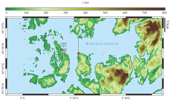
Figure 1.
Location of the three pulsed wind lidars (triangles) in the Bjørnafjord and location of the planned fjord crossing (dashed line).
Three long-range Doppler wind lidars, named Whittle, Koshava, and Sterenn, were deployed in the Bjørnafjord in May 2016 (Figure 1). Each lidar unit is a modified WindCube 200S from Leosphere (Orsay, France), the main properties of which are given in Table 2, based on the information provided by Vasiljevic et al. [17]. In the following, the lidar Sterenn is referred to as Lidar East (LE), whereas the lidars Whittle and Koshava are referred to as Lidar West 1 (LW1) and Lidar West 2 (LW2), respectively.
Table 2.
Characteristics of the modified WindCube 200S used in the long-range WindScanner system during the Bjørnafjord measurement campaign.
The lidars LW1 and LW2 are on the west side of the fjord, at an interval of few meters. Their latitude and longitude is, therefore, assumed identical and set to 60.0878° and 5.2653°, respectively. The lidar LE is installed some kilometres to the South-East of LW2 and LW1, with a latitude of 60.0836° and a longitude of 5.3608°. The scanning head of the lidars LW2 and LW1 is oriented toward the East, whereas the scanning head of LE is oriented toward the North-West (Figure 2).
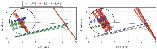
Figure 2.
(left) North-South (N-S) scanning configuration; (right) East-West (E-W) scanning configuration.
2.2. Scanning Configurations
Two different configurations were adopted in the present study. Data acquired with the first one, called “North-South configuration” (N-S configuration), are utilized for the analysis of the wind spectrum (left panel of Figure 2). This configuration was originally set up to study the wind coherence for a flow from the East but turned out to be used for the analysis of the single-point spectra only since the wind ended up coming from north-northwest. Data from the second configuration, named “East-West configuration” (E-W configuration), are used to study the wind coherence for flow from north-northwest (right panel of Figure 2). Therefore, the two data sets investigated are disjoint and may correspond to different atmospheric conditions.
For the N-S configuration, the lidars LW1 and LE use a Line-Of-Sight (LOS) scanning mode, also called staring mode, where the azimuth angle and the elevation angle are fixed, with a sampling frequency . The lidar LW2 uses a “discrete” Plan Position Indicator (PPI) sector scan, which can be seen as an improved PPI sector scan, the latter being defined as a continuous scan with varying azimuth angles and a fixed elevation angle. If the measurement is not interrupted during the motion of the scanning head, the retrieved velocities are not only spatially averaged along the scanning beam, but also along the arc drawn by the scanning pattern. This motion-induced spatial averaging may be detrimental for the measurement of the lateral wind coherence, especially at a large scanning distance. The discrete PPI sector scan used in the present study avoids such a motion-induced spatial averaging by interrupting the measurements during the motion of the scanning head. The discrete PPI sector scan is conducted using four different azimuth angles within a narrow sector. Consequently, the wind data recorded by LW2 are sampled at ca. 0.22 , which is slightly less than the theoretical value of 0.25 . The difference is due to the time it takes for the scanning beam to move from one position to another.
For the E-W configuration, LW1 and LW2 utilize a Line-Of-Sight (LOS) scan towards East, whereas LE uses the discrete PPI sector scan. The details of each scan are provided in Table 3. Although Table 3 shows that the range gate is 75 , they overlap near the intersection of the different scanning beams, as illustrated by the reduction of the apparent range gate spacing in Figure 2.
Table 3.
Azimuth angles, elevation angles, maximal range and sampling frequency at which the wind data are recorded for each lidar configuration.
2.3. Data Processing
In the following, u, v and w represent the along-wind (x-axis), the crosswind (y-axis) and the vertical (positive z-axis) wind components, respectively. The projection of the wind velocity vector onto the scanning beam of a lidar unit is denoted . Each velocity component can be decomposed into a mean component, denoted by an overline and a fluctuating component with zero mean denoted by a prime:
where ms [19]. Unless the scanning beam is perpendicular to the flow, the mean velocity of the along-beam component verifies ms.
In the adopted scanning cycle, data at five different lidar beam intersections are recorded. Four of the “points” are monitored with a frequency of 0.22 , while the last intersection, where both lidars are in a staring mode, is observed with a sampling rate of 1 . The use of a common sampling frequency between the different lidar units is a necessary condition to retrieve the two horizontal wind components. The along-beam velocity component of each lidar unit is first resampled up to 1 , using linear interpolation with query points. Then, the two horizontal wind components are retrieved with a sampling frequency of 0.22 . Using a sampling frequency of 0.22 instead of 1 is not observed to alter the turbulence statistics discussed in the present study. This is partly because the along-beam spatial averaging (ABSA) of the velocity data leads to a truncation of the wind spectrum above 0.22 (cf. Section 3.3). More details about the ABSA are given in Section 2.6.
Assuming the elevation angles are small enough to be neglected, only two lidar units can be used to retrieve the two horizontal wind components:
where and are the azimuth angles of each lidar; and refer to the along-beam wind component of each lidar; and are the northern and eastern wind components, respectively. The along-wind and crosswind components are then estimated using:
where is defined as:
The data are analysed using an averaging time of 10 and outliers are removed using a Hampel filter [20], with a window length of 240 and 5 standard deviations away from the local median. Figure 3 illustrates the retrieval of the two horizontal wind components, using LW2 and LE, with the E-W configuration. The azimuth angles selected are equal to 324.4° and 76.5° for LE and LW2, respectively. The wind direction associated with the selected sample is 311°, which means that the beam of LE recorded mostly the along-wind component. Figure 3 shows clearly that the sampling frequency of the time series recorded with LE is larger than with LW2. This results in an along-wind component that seems to be described with a better time resolution than the crosswind component.
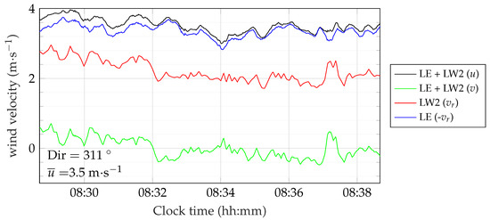
Figure 3.
Along-beam velocity component recorded by the Lidar West 2 and the Lidar East on 2016-06-07 (East-West configuration), and corresponding retrieved horizontal wind components.
The data availability is defined here as the percentage of time series of 10 duration from which the mean velocity can be estimated. For the E-W configuration, this results in a data availability of ca. 46% for the combination of LW2 and LE and a data availability of ca. 19% for the combination of LW1 and LW2. For the N-S configuration, the data availability is equal to 46% for the combination of LW2 and LE and 7% for the combination of LW1 and LE. Because LW1 is usually responsible for the low data availability, only data measured using LW2 and LE are considered in the following.
2.4. Turbulence Model Based on the N400 Handbook
2.4.1. Wind Spectra
The wind spectra presented in the following are one-sided, i.e., their integral from a zero frequency to infinity is equal to the variance of the corresponding wind component. The Handbook N400 [9] follows the EN 1991-1-4 [18] definition of the mean wind velocity profile and turbulence intensity profile, as a function of five terrain categories and based on an averaging time of 10 . Following the Handbook N400, the relationship between the turbulence intensity of the along-wind, crosswind and vertical wind components, denoted , and , respectively, is:
The turbulence intensity described in the Handbook N400 is defined as:
where is a minimum wind profile height, which depends on the terrain category, described in EN 1991-1-4 [18].
Given three constants , and , the single-point wind spectra () are:
where () is the integral length scale, defined as:
where is a reference length scale equal to 100 and a reference height equal to 10 , as prescribed in EN 1991-1-4 [18].
2.4.2. The Wind Coherence
The coherence is the normalized cross-spectral density of the wind velocity fluctuations measured in two different positions. It has been used since the 1960s to take into account the spatial correlation of the wind gusts [21,22,23] and is, therefore, a key element of the buffeting theory [24,25]. The lateral root-coherence is defined as the modulus of the root-square of the lateral coherence:
where f is the frequency; and are the single-point wind spectra measured in two positions and , respectively; is the cross-wind separation and is the cross-spectrum for the i-component. The coherence consists of a real part (the co-coherence) and an imaginary part (the quadrature spectrum). Since the imaginary part is often small and the in-phase wind action is more important for wind loading modelling, the co-coherence is commonly approximated by the root-coherence.
Following the Handbook N400 [9], the co-coherence is approximated by an exponential decay function, proposed first by Davenport [22] and referred to as the “Davenport coherence model”:
where is the horizontal mean wind velocity; , and is a “decay parameter”, defined in Table 4. It should be noted that the decay parameter found in the literature is highly scattered with estimates ranging from 3 to more than 20 [26].
Table 4.
Decay coefficients provided by the Handbook N400 [9] for the coherence model in Equation (14).
For a large crosswind separation , the ratio (where L is a typical length scale of the turbulence) cannot be considered small and the coherence becomes less than unity at zero frequency [27]. This is not accounted for in the Davenport coherence model, which results in an overestimation of the fitted decay coefficient. Therefore, more realistic coherence models are required. A two-parameter exponential function can, for example, be used:
where and are coefficients to be determined by fitting the function in Equation (15) to the estimated co-coherence. However, the coefficient is dimensionless, and has the dimension of the inverse of a time. Equation (15) can be re-written as:
In Equation (16), has the dimension of a distance and is proportional to a length scale:
Coherence models similar to Equation (16) have been proposed by e.g., Hjorth-Hansen et al. [28] and Krenk [29]. If , then Equation (15) reduces to the Davenport coherence model. A more complex 4-parameter exponential decay function (Equation (18)) has been used to model the wind coherence in another Norwegian fjord [14]. Such a model is not used to estimate the lateral coherence in the present study because the limited amount of data, the low coherence measured and the large crosswind separations do not allow an accurate estimation of the two additional parameters and . The parameter is, however, adapted for the study of the coherence when the wind direction is not perpendicular to the array of measurement volumes [14] and can be related to the “phase angle” used in e.g., ESDU 86010 [30]:
2.5. The Frøya Wind Spectrum
The NORSOK Standard [10] uses the wind spectrum developed by Andersen and Løvseth [31], which is based on the measurement campaign on Sletringen island (Frøya municipality) at the Norwegian coast. This wind spectrum is defined at an arbitrary altitude z for the along-wind component only. It was established using time series of 40 duration and a mean wind velocity measured 10 above sea level:
In the present study, the mean wind velocity is calculated using measured at and assuming that the logarithmic profile applies, i.e.,:
where is the terrain roughness.
The equation used by Andersen and Løvseth [32] to estimate the turbulence intensity from the Frøya database is:
2.6. Spatial Averaging Effect of the WindCube 200S
A Doppler wind lidar measures the wind velocity in a volume stretched along the scanning beam. Consequently, the recorded along-beam velocity is a low-pass filtered version of the related point velocity. Modelling the spatial averaging is fundamental in evaluating to what extent the wind turbulence measurements are affected by the instrument performance. Such a modelling allows, for example, to estimate the measurement bias in the standard deviation of the wind velocity. For the wind velocity spectrum, it is also of great interest to know above which frequency the along-beam spatial averaging (ABSA) is no longer negligible.
The ABSA effect can be expressed as a convolution between the spatial averaging function and the vector of the wind velocity , at a focus distance r from the lidar. The along-beam wind velocity is, therefore, written as:
where is a unit vector along the beam and s is the integration variable that has the dimension of a distance. If the scanning beam is aligned with the wind direction, then Equation (24) can be directly calculated using a scalar convolution product. For a pulsed wind lidar such as the WindCube 200S, can be modelled as [16]:
where l is the range gate size, i.e., the range within which the lidar signals are measured. The spectral transfer function H corresponding to the spatial averaging function is:
The standard deviation of the along-wind component calculated as a function of the spectral transfer function is then:
If there is no ABSA, then the standard deviation of the along-wind component observed in a single-point is denoted :
The relative deficit in due to the ABSA plotted in Figure 4 is therefore:
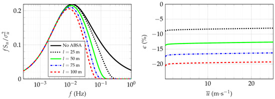
Figure 4.
(left) influence of the along-beam spatial averaging (ABSA) effect of the WindCube on the measured normalized spectrum defined in the Handbook N400, using an arbitrary mean wind velocity 10 s at ; (right) estimation of the corresponding deficit of the estimated standard deviation of the along-wind velocity due to the ABSA.
To illustrate the influence of the ABSA on the wind spectrum of the along-wind component , the latter is estimated using 10 s and 25 , following the wind spectrum model adopted in the Handbook N400. The wind spectrum is filtered using the spectral transfer function (Equation (26)) for different range gate sizes, from 25 to 100 , and displayed on the left panel of Figure 4. The right panel of Figure 4 shows that, for 10 s, the standard deviation of the along-wind component may be underestimated by 8.3% if and 16.6% for because of the ABSA. If is calculated for using the variance instead of the standard deviation, then . For the field measurements conducted in the Bjørnafjord, the value of l was set to 75 so that the WindScanners could measure the flow at larger distances. Although Figure 4 provides an overall indication of the ABSA effect, the deficit depends actually on additional parameters, such as the angle between the wind direction and the scanning beams and the measurement noise.
3. Results
3.1. Preliminary Comparison with a Sonic Anemometer on Land
Although there is no reference sensor available in the fjord allowing a direct assessment of the data recorded with the multi-lidar configuration, two meteorological masts were installed at the end of 2015 by the company Kjeller Vindteknikk AS (Kjeller, Norway), abbreviated KVT in the following, on the island of Ospøya. This island is located ca. 2.3 North of LW2. The southernmost mast is 50 high and installed at a height of ca. 35 above the mean sea level. This mast is equipped with one Gill WindMaster Pro 3-axis sonic anemometer (Lymington, Hampshire, UK) at a height of 67 and two others located at 83 above the mean sea level. The three sonic anemometers operate at a sampling frequency of 10 . The mast and the data gathered by the sonic anemometers are owned by KVT. Therefore, a detailed analysis of the mast instrumentation and its measurement data is out of the scope of the present study. Nonetheless, during the last four days of the measurement campaign, LW2 conducted a fixed LOS scan toward the mast, with an elevation angle of 1.85°. KVT provided velocity measurements from the sonic anemometers so that a comparison with the lidar data could be conducted in terms of mean value and standard deviation of the along-beam velocity component. To the authors’ knowledge, the sonic temperature measurement data were, however, not stored. For the sake of brevity, only data recorded by the sonic anemometer installed at the altitude of 83 are considered in the following. At the scanning distance of 2.3 , the range gate closest to the met mast is at a height of ca. 75 above the mean sea level.
To simplify the comparison between the velocity data recorded by the lidar and the sonic anemometer, the along-beam component is considered. For the sonic anemometer, is estimated using:
where is the azimuth angle; is the elevation angle and is the wind direction, as defined in Equation (7). Figure 5 shows that the 1 -averaged along-beam velocity component is remarkably well captured by LW2. A more detailed comparison of the two device performances is provided in Figure 6. The best linear fit between the mean wind velocity of the along-beam component recorded by LW2 and the sonic anemometer shows a squared correlation coefficient of and almost no bias. For the standard deviation, the squared correlation coefficient is also significantly large and equal to , but a systematic discrepancy is observed between the lidar data and the sonic anemometer data, which is expected and attributed to the spatial averaging effect. The results presented in Figure 5 and Figure 6 are not surprising, as a similar comparison with sonic data has already been done in the past by Pauscher et al. [7]. Nevertheless, the comparison given herein shows that the wind data recorded by the multi-lidar system in the Bjørnafjord and presented in the following are reliable.
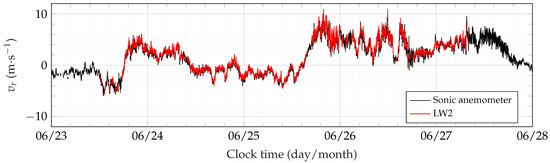
Figure 5.
Along-beam velocity recorded during the last four days of the measurement campaign by LW2, and the sonic anemometer located 2.3 North of the lidar unit, at a height of 83 above the mean sea level. For illustrative purposes only, the sampling time is increased to 1 .
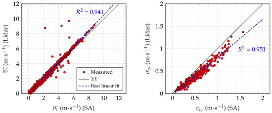
Figure 6.
Ten-minute averaged mean velocity (left) and standard deviation (right) of the along-beam component recorded by LW2 (vertical axis) and the sonic anemometer (horizontal axis), at , during the last four days of the measurement campaign.
3.2. Statistical Moments
The wind roses displayed in Figure 7 for the E-W configuration (left) and the N-S one (right), represent the wind data recorded by the long-range WindScanners in the laser-beam intersection volume generated by LE and LW2. In both cases, the majority of wind records represents a wind direction from north-northwest, i.e., almost aligned with the scanning beam of LE, with wind velocities up to 17.7 s for the N-S configuration and up to 13.8 s for the E-W configuration. For wind velocities above 8 s, the average values of and estimated using the N-S configuration are 0.056 and 0.042, respectively. For the the E-W configuration, and are in average equal to 0.043 and 0.030, respectively. The ratio is, therefore, equal to for the E-W configuration and for the N-S configuration, which is in the range of expected values [26]. The low turbulence intensity recorded here may not be explained by the ABSA influence alone, although that effect does result in an underestimation of the standard deviation of the wind velocity and thereby an underestimation of the turbulence intensity.
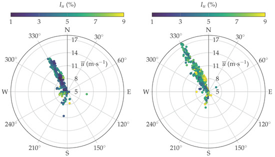
Figure 7.
(left) Ten-minute mean wind velocity, direction and turbulence intensity recorded from 18 May 2016 to 21 June 2016 with the E-W configuration (326 samples with ms); (right) Ten-minute mean wind velocity, direction and turbulence intensity recorded from 2016-06-07 to 2016-06-22 using the North-South configuration (437 samples with ms).
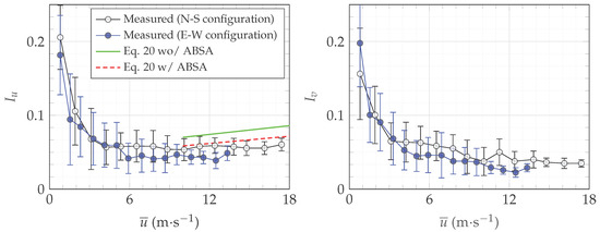
Following Equation (9), which is defined for a neutral stratification, a roughness length of 0.003 and an altitude of 25 above sea level gives a turbulence intensity of 0.11. A roughness length as low as 0.0001 has been reported for flows over the sea at moderate wind speeds [33,34]. For , the turbulence intensity calculated according to EN 1991-1-4 [18] and corrected for the ABSA is , which is much closer to the values recorded during the measurement period. For this reason, turbulence statistics assuming a roughness length are investigated in the following. At low wind velocities, statistical measures defined primarily for shear generated turbulence are estimated with large uncertainties. This is mainly due to the increasing number of non-stationary samples, related to increased convective mixing and buoyancy effects, and to less extent, to increasing errors in the lidar measurements. In Figure 8, one can see that the turbulence intensity estimates become steady for a mean wind velocity around 6 ms. In the following, the estimated turbulence intensity is therefore discussed for ms, i.e., for wind velocities large enough to provide consistent wind statistics.
A rigorous estimation of the atmospheric stability relies on measurements of vertical fluxes of momentum and heat. This can be done using either a meteorological mast instrumented with cup anemometers, temperature and humidity sensors [35] or a 3D sonic anemometer able to measure the sonic temperature [36,37]. In the present case, such an instrumentation was not available, and no measurement of the vertical profile of mean wind velocity above the sea surface could be conducted using the lidars, due to the low elevation angles used. Therefore, alternative methods are considered in the present study to discuss possible effects of a non-neutral atmosphere on the lidar measurement data.
The low turbulence intensity observed may be partly due to a stable atmospheric stratification, for which values lower than were recorded at a height of 70 above the sea level and for ms in an offshore environment by e.g., Hansen et al. [38]. Previous studies conducted at bridge sites in coastal areas have also reported a turbulence intensity close to or below 0.06. Sacré and Delaunay [39] measured at for moderate winds from the sea (11.6 s to 15.7 s) and a neutral stratification. For a seasonal wind, Toriumi et al. [40] measured a turbulence intensity close to 0.04 at for a mean wind velocity of about 23 s, which is strong enough to assume that mechanically-generated turbulence was dominating over buoyancy effects.
For ms, the standard deviation of the wind direction is lower than 3.75 (N-S configuration) and 2° (E-W configuration) for 80% of the wind samples. According to Sedefian and Bennett [41], such a low standard deviation may correspond to a slightly stable atmospheric stratification. Nonetheless, the low standard deviation of the measured wind direction may also result from the ABSA effect. Figure 8 indicates that a stable atmosphere may have been predominant during the monitoring with the E-W configuration since the turbulence intensity measured for ms is systematically lower than for the N-S configuration, whereas the wind direction is almost the same (Figure 7). For ms, the turbulence intensity seems to be rather constant, whereas Equation (23) leads in Figure 8 to a clear increase of the turbulence intensity with the mean wind velocity. This suggests that the roughness of the sea in the Bjørnafjord is not clearly increasing with the mean wind velocity, as typically observed in an offshore environment.
The uncertainties regarding the atmospheric stability observed during the measurement campaign highlight the need to associate the lidar data to measurements from weather stations and sonic anemometers on land.
3.3. Wind Spectra Comparison
Each individual spectrum is estimated using the periodogram power spectral density (PSD) estimate with a Hamming window, which corresponds to the particular case of Welch’s algorithm with a single segment. We chose to use a single segment so that the wind spectrum can be described down to a frequency of 0.0017 . To reduce the large random error that results from the use of the periodogram PSD estimate, the different spectra are ensemble averaged. An additional smoothing of the PSD in the high-frequency range is done using non-overlapping block average with 60 blocks that are equally spaced on a log scale.
The PSD estimate of the along-wind component is displayed on the left panel of Figure 9, whereas the right panel shows the PSD estimate of the along-beam component recorded by LE. In both panels, only samples characterized by a mean wind velocities between 11 s and 18 s are considered, but only the ensemble averaged PSD estimates are displayed for the sake of clarity. The relatively large velocity range selected justifies the use of the wavenumber (left panel) or (right panel) instead of the frequency. The wind spectra are pre-multiplied by the wavenumber and divided by the variance of the corresponding wind velocity component. For 11 ms ms, the wind direction is on average equal to 330° (Figure 7), and the along-beam component is, therefore, almost equal to the along-wind component. Assuming the flow is uniform in the middle of the fjord, was calculated using the data gathered at scanning distances ranging from 2 to 3.5 , i.e., 15 different range gates. This results in a slightly smoother wind spectrum at every frequency than for the PSD estimate of the along-wind component.
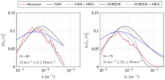
Figure 9.
Normalized wind spectrum recorded using both data recorded by LW2 and LE from the 07-06-2016 to 22-06-2016 (left panel) and LE alone (right panel) for the N-S configuration.
The wind spectra from the Handbook N400 and NORSOK standard are calculated for and superimposed to the measured PSD. The normalization of the spectra by the variance of the wind velocity allows, in particular, a reduction of the uncertainty related to the estimation of the roughness length. For the NORSOK and N400 spectra, is estimated using Equation (28). However, the lidar data is known to be associated with underestimated values of and . Therefore, and were estimated directly from the time series, and a correcting coefficient was introduced, assuming an underestimation of ca. 30%, as suggested by Figure 4.
In Figure 9, the measured spectral peak and the one estimated using the NORSOK spectrum are well aligned. The spectral peak of the N400 spectrum is located at a slightly higher wave-number than the measured one. For , the NORSOK spectrum gives higher spectral values than observed from the recorded data. This is not unreasonable, as other studies [42,43] have shown that wind spectra measured offshore often contain more energy at low frequencies compared to the wind spectra measured onshore. This is partly due to the fact that, in an offshore environment, the size of eddies is not limited by topographical changes. Although the flow from north-northwest recorded in the Bjørnafjord comes from the ocean, it is likely affected by the islands upstream of the monitored domain as well as the shoreline of the fjord. Consequently, an offshore wind spectrum model, such as the one used in the NORSOK standard may overestimate the spectral values at low wave-numbers. The discrepancies between the measured spectrum and the NORSOK spectrum may also be related to a slightly stable atmospheric stratification. For ms, Andersen and Løvseth [44] observed a negligible difference between the Frøya spectrum measured in stable and neutral stratification. On the other hand, Mann [45] found strong effects of stability on spectra over the Great Belt, Denmark, up to over 16 s, albeit at a height of 70 .
When the high-frequency range of the N400 wind spectrum is attenuated using the ABSA model presented in Equation (26), the slope of the high-frequency part of the modified spectrum is sharper than measured, as seen in Figure 9. Similar observations have been reported by e.g., Pauscher et al. [7] with the long-range WindScanner system or e.g., Angelou et al. [46] with the short-range WindScanner system. The discrepancies between the modelled ABSA and the measured one may be due to fluctuations of the wind direction and the use of multiple scanning beams to retrieve the horizontal wind components. For frequencies above 0.22 and 14 ms, i.e., wave-numbers above 0.10, the right panel of Figure 9 shows that the PSD of the along-beam wind velocity component is considerably attenuated by the ABSA, viz. The high-frequency turbulent components are under-represented in the lidar data.
Figure 10 shows the spectrum, estimated without normalization by . Consequently, the wind spectra need to be split into several velocity bins, since a different mean wind velocity now has a significant effect on the magnitude of the PSD estimate. The study of allows the assessment of an appropriate roughness length for the N400 spectrum. The spectra displayed in Figure 10 are, therefore, complementing those displayed in Figure 9. In Figure 10, the N400 spectra is estimated with , which is 30 times lower than proposed in the Handbook N400. Nevertheless, it leads to a fairly good agreement between with the measured wind spectra, especially for ms. The NORSOK spectrum is found to systematically overestimate the PSD of the along-wind velocity component, which is likely due to the fact that this spectrum is site-specific.
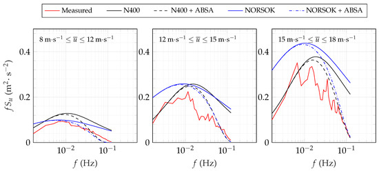
Figure 10.
Power spectral density estimate of the along-wind velocity component recorded using both data recorded by LW2 and LE from the 07-06-2016 to 22-06-2016 (N-S configuration), using .
3.4. Coherence Estimated from the Full-Scale Wind Measurements
The estimation of the lateral wind coherence using synchronized long-range wind lidars is challenged by the large scanning distances. By using the short-range WindScanner system and a smaller range gate (), Cheynet et al. [14] observed a negligible influence of the ABSA on the wind coherence measurement. For , the ABSA may, however, affect the estimation of the wind coherence to a larger extent. However, because the range resolution of a continuous wave lidar increases quadratically with the scanning distance [46], the short-range WindScanner cannot be used to monitor the flow at large scanning distances.
3.4.1. Longitudinal Coherence of the Along-Wind Component
Since one of the lidar beams in the E-W measurement configuration more or less pointed in the mean wind direction, wind velocity records along the beam provide a unique opportunity to revisit Taylor’s hypothesis of frozen turbulence [47], in relation to the estimation of the along-beam coherence. For this purpose, the lidar data acquired by LE alone with a yaw angle as small as possible, i.e., are selected. This implies that the mean wind direction considered is the same as that of the lidar beam.
Wind records in five range gates, at distances from to from the lidar are considered. In the present case, the longitudinal separation, denoted in Figure 11, ranges from 100 to 400 , which is significantly larger than in previous field measurements [48,49]. For a perfectly frozen turbulent flow moving toward the lidar, the wind data, which are simultaneously recorded at different range gates, are distinctly out of phase because the flow recorded in a given range gate is a “delayed version” of the flow recorded upstream.
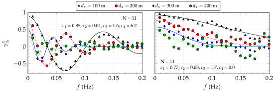
Figure 11.
Measured (markers) and fitted (lines) along-beam coherence, obtained using the staring Line-Of-Sight scan of the Lidar East (North-South configuration), with 10 ms 15 ms, a yaw angle , without (left) and with (right) synchronization of the time series considering a time lag equal to .
The negative values in the co-coherence function in the left panel of Figure 11 reflect such an out-of-phase appearance of the wind gusts, not accounted for by the Davenport coherence model. The 4-parameter coherence function (Equation (18)) is, therefore, fitted to the measurement data. The estimated value of is very close to , which is the expected value, provided Taylor’s hypothesis is applicable, according to ESDU 86010 [30]. For a perfectly frozen turbulent field, the decay coefficient in the Davenport model or in Equation (18), should be equal to 0. The 4-parameter function is also fitted to the modified “co-coherence” of the along-wind velocity, where the wind data are “synchronized”, as if they were observed at a single point (right panel of Figure 11). This synchronization was done by introducing a time lag equal to in the lidar data at the four range gates considered. Relatively close values of the coefficient can be observed in both panels. In the present case, .
If the Davenport model is fitted to the modified “co-coherence” displayed on the right panel of Figure 11, we obtain . Together with in the 4-parameter coherence model, it provides an indication of the relevance of Taylor’s hypothesis. For the conditions in the middle of a 5 wide fjord, with a fetch across water of several kilometres in each direction, a low turbulence intensity and a sampling frequency of 0.22 that limits the focus of the Lidar measurements to the large scale fluctuations, Taylor’s hypothesis is expected to be more valid than in many other instances, for which values ranging from 1.0 to 10 were reported [26,48,49].
3.4.2. Lateral Coherence of the Longitudinal Wind Fluctuations
Assuming that Taylor’s hypothesis of frozen turbulence is applicable and the wind direction is perfectly aligned with the beam orientation, the lateral coherence should be unaltered by the ABSA effect [14]. Although relevant, the investigation of the lateral coherence in the case where the wind direction and the scanning beams are not aligned is out of the scope of the present study. In the following, the coherence is, therefore, handled as unaltered by the ABSA.
Using the E-W configuration (Figure 2), the scanning beams intersect in eight positions, i.e., were intended to provide data from eight different measurement volumes. Unfortunately, only four of them could be used because the overall data availability from LW1 was insufficient during the measurement campaign.
The co-coherence is estimated from stationary wind velocity records using Welch’s method [50] with a sample duration of 10 and six segments with 50% overlapping. The number of overlapping segments is chosen to reduce the bias of the coherence estimate and the measurement noise [51,52] while keeping the frequency resolution as high as possible. Wind data with a mean wind velocity between 6 s and 14 s are considered (189 samples) and the coherence is expressed as a function of the wavenumber k to reduce the scatter of the coherence estimates due to the dependence of the lateral coherence on wind velocity. The measurement of the lateral coherence requires a flow perfectly perpendicular to the different volumes monitored, i.e., a yaw angle equal to zero. To keep the influence of the yaw angle on the coherence low, only wind data with a mean wind direction between 317° and 337° are selected. This corresponds to a maximal yaw angle of 10° with respect to the average azimuth angle of LE (Table 3). A non-zero yaw angle introduces a non-zero phase in the wind data and a lateral separation that is shorter than measured. The Davenport co-coherence of the along-wind component can be expressed in the horizontal plane as a function of the yaw angle:
It can be shown that for a yaw angle of 10° and small values of compared to , Equation (31) can reduce to:
For the lateral separations considered, the coherence is usually low and contaminated by measurement noise for frequencies above 0.06 . The curve fitting procedure uses, therefore, only data from the frequency range below 0.06 . The measured wind coherence is fitted, in the least-square sense, using the two-parameter exponential decay function (Equation (15)).
Figure 12 shows the average coherence estimated for six different lateral separations. The relatively low number of data points with significantly high coherence leads to some uncertainties regarding the parameter . A coherence lower than 1 at zero frequency may be expected for large lateral separations [27], which would correspond to a value of between 0.01 and 0.2 as observed in the Lysefjord [54]. In the present case, the coefficient is the same as the decay coefficient of the Davenport coherence model because the value of is close to 0 . The measured exponential decay parameter is larger than the one given in the Handbook N400 as well as the values found in the literature for a flow measured above the sea with a low turbulence intensity (Table 5). It should be noted that the coefficient given in Table 5 for the study of Toriumi et al. [40] is the value estimated by fitting the Davenport Model to the data provided in their research article. The coherence measured by Andersen and Løvseth [32] is well approximated by Davenport coherence model but is considerably lower than in any other studies found in the literature with a decay parameter equal to 64. If Equation (15) is applied to the data point provided in Andersen and Løvseth [32], then and . The reason for such a low coherence estimate remains unclear.
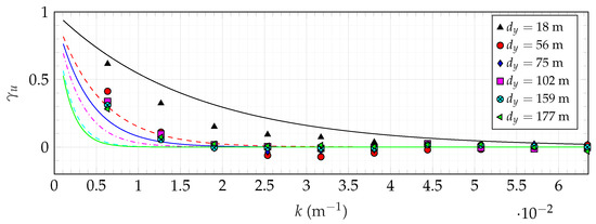
Figure 12.
Measured (scatter plot) lateral wind coherence of the along-wind component recorded using the data from LW2 and LE from 18 May 2016 to 21 June 2016 (E-W configuration) fitted with Equation (15) (smooth lines).
Table 5.
Decay coefficients available in the literature, obtained from full-scale measurements of the wind coherence along a suspension bridge crossing a fjord, an estuary or a strait.
3.5. Coherence Estimated from Single Lidar Data
Comparison with the Two-Parameter Coherence Function
In the present case, if only the data recorded by LE are used with an along-beam mean velocity ms, the wind direction is mostly from north-northwest (Figure 7). Here, only samples characterized by 10 ms 14 ms are, therefore, considered. Because a pulsed wind lidar measures simultaneously the wind velocity in several positions along the scanning beam, the lateral wind coherence can be estimated at several scanning distances from the lidar unit. For each range gate, the wind co-coherence was, therefore, calculated and fitted by a two-parameter exponential decay function, using four measurement volumes, the spacing of which increases for increasing scanning distances.
In Figure 13, the measured coherence is presented for and . The scanning distance corresponds to the location monitored jointly by LW2 and LE, as discussed in the previous section. Although the coherence decreases for increasing lateral separations, the reduction is rather limited for separations beyond ca. 40 , for both and . In the case of a scanning distance of , the measured coherence at varies between 0.27 and 0.37 for ranging from 46 to 157 . Similarly, the lateral co-coherence estimated by Toriumi et al. [40] is not well modelled by the Davenport coherence model and displays a limited dependency on at large cross-wind separations. The limited “sensitivity” of the coherence function to lateral separations larger than 40 may be related to the fact that, in general, the coherence becomes weak at such separations. The estimated coefficient governing the fitted coherence function is consistent with the one based on LW2 and LE data.
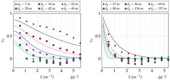
Figure 13.
Measured (markers) and fitted (Equation (15), lines) co-coherence using data recorded by the four scanning beams of LE only (E-W configuration), at a scanning distance (left panel, using 84 samples) and (right panel, using 93 samples), with 10 ms 14 ms, from 18 May 2016 to 21 June 2016.
In Figure 14, the coefficient varies from ca. 20 to 28 for the different scanning distances and is relatively constant for . For , the cross-wind separation ranges from 7 to 49 , whereas, for , it ranges from 23 to 157 . The fluctuations of the coherence and the decrease of the coefficient with r reflects the increasing difficulty to estimate the wind co-coherence at greater scanning distances and larger lateral separations. The variation of the coefficient is also expected to partly reflect the physical change of the flow conditions closer to land. More generally, Figure 13 suggests that the functional form of the Davenport coherence model may not be suitable for the coherence measured in the Bjørnafjord.
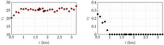
Figure 14.
Coefficients of the two-parameter wind coherence function fitted to the wind coherence measured from 18 May 2016 to 21 June 2016 using LE only (E-W configuration), with 10 ms 14 ms and .
3.6. Application of an Alternative Coherence Model
The more complex dependency of the measured co-coherence on the lateral separation may be modelled using Bowen’s coherence model [55], which is derived from the Davenport coherence model, except that the decay parameter has the following form:
where and are two coefficients to be determined and z is the measurement height. The function is an idealized representation of the lateral coherence of the along-wind turbulence near the ground. Bowen et al. [55] arrive, for example, at and . In the present case, and are determined using a least-square fit to the measured co-coherence. Minh et al. [56] proposed a more complex three-parameter coherence model, which also depends on and , but is independent of the measurement height. For the sake of simplicity, only the Bowen model is investigated in the following.
Figure 15 shows that the Bowen coherence model seems to provide a much better fit to the measured coherence than the Davenport coherence model at both and . Figure 16 shows, however, that the fitted coefficients display a large variability at . This is likely due to the fact that the coherence seems to become independent of for and the majority of the cross-wind separations are larger than 50 for . The low dependency of the estimated co-coherence on at large crosswind separations is reflected in the negative value of that counterbalances , as shown in the right panel of Figure 16.
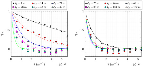
Figure 15.
Same as Figure 13, except that the solid and dashed lines correspond to the coherence model derived from Bowen et al. [55].
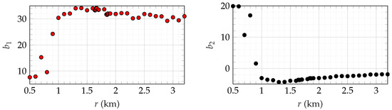
Figure 16.
Coefficients of the Bowen coherence model fitted to the wind coherence measured from 18 May 2016 to 21 June 2016 using LE only (E-W configuration), with 10 ms 14 ms and .
The Bowen coherence model suggests that the coherence depends on the measurement height z and , which is not predicted by the Davenport coherence model. To estimate the wind load on a suspension bridge, the measurements should, therefore, be conducted at the deck height. Because the Bowen coherence model was designed at an altitude lower than 20 , it is uncertain beyond which height such a model ceases to be valid. Measurement in a narrower Norwegian fjord reported in ([54], chapter 2), conducted at a height of 60 for a wind speed above 8 s, showed, for example, that a coherence model that is simply scaled by was sufficient to properly capture the lateral wind coherence of the along-wind component.
4. Discussion
4.1. Determination of a Site-Specific Wind Spectrum
In the present study, the range gate of 75 introduces a large ABSA that prevented a detailed analysis of the wind spectrum for frequencies above 0.03 Hz. A site-specific single-point spectrum may be developed by combining sonic anemometer and lidar measurement data so that the ABSA can be better modelled. Once this challenge is overcome, the determination of the first two statistical moments of the longitudinal wind component ( and ) and the integral length scale may allow the application of e.g., the von Kármán spectrum [57] as a site-specific wind spectrum.
The turbulence spectra provided in the wind loading sections of several standards (e.g., [9,18]) are characterized by the same spectral form as the von Kármán spectrum model. When these spectra are pre-multiplied by the frequency, they follow a power law in the high-frequency range (inertial subrange) and a power law at low frequencies. The smooth junction between these two frequency ranges is done through a spectral peak, centered at a frequency around . However, there is evidence of the existence of a plateau instead of a spectral peak [58,59], for both the crosswind and longitudinal wind components. For the latter component, the width of the plateau increases at decreasing altitudes. For a floating bridge with pontoons, typically characterized by a low altitude above sea level, an erroneous modelling of the structural response may be accentuated by the use of the so-called “blunt” and “pointed” models [60], which do not predict the existence of such a plateau.
4.2. Environmental Effects on the Estimated Coherence
The decay coefficients and provided by the Handbook N400 (Table 4) are almost the same as those obtained from the full-scale measurements conducted by Jensen and Hjorth-Hansen [53] in 1977 on the Sotra Bridge, for a neutral stratification, at an altitude of 60 above the sea level. This bridge crosses a narrow fjord located ca. 40 on the North-West of the Bjørnafjord. The discrepancies between the estimated decay coefficients and those predicted by the Handbook N400 may therefore be explained by the following reasons:
- The atmosphere may have been predominantly stable during a part of the measurement campaign. In particular, a stable stratification leads to a lower coherence than for a neutral atmosphere. Ropelewski et al. [49] suggested that it may result from the reduction of the lateral size of the eddies with respect to their longitudinal size. Following Panofsky and Mizuno [61], the decrease of the wind coherence with increasing stability is, however, only valid for cross-wind separations larger than 50 .
- Ropelewski et al. [49], Kristensen and Jensen [27] or Sacré and Delaunay [39] observed that decreases for increasing heights. It is, therefore, not surprising if the lateral co-coherence estimated at is lower than the one at , as measured by Jensen and Hjorth-Hansen [53]. Such an evolution of the coherence is expected and may reflect the increasing size of the eddies with the altitude [62,63].
- The estimation of the coherence using large crosswind separations is more challenging than with small separations. That is one of the reasons why Kristensen and Jensen [27] considered only relatively small lateral separations. If a coherence model with a single parameter is used, the decay coefficient may increase for increasing cross-wind separations, especially in stable or near-neutral atmosphere [61,64]. This issue is taken into account in the present study, where the 2-parameter exponential decay function (Equation (15)), which relies on an additional parameter , was used instead of the Davenport model. However, the coherence was likely not sufficiently large to accurately estimate . For wind load estimation on a bridge deck, a more rigorous comparison between the coherence measured in a wide fjord and the one provided in the Handbook N400 should, therefore, be undertaken by considering both small and large cross-wind separations in conjunction with observations of the atmospheric stability.
4.3. Environmental Effects on the Flow Uniformity
The influence of the nearby islands and the coastal terrain on the turbulence statistics studied can be briefly assessed using the along-beam mean wind velocity and its standard deviation for the case of a flow from North-West. Figure 17 shows that the mean velocity estimated using LE is rather uniform for both the N-S and E-W configurations, whereas the standard deviation decreases for increasing scanning distances. LW2 measures with a larger dispersion for the N-S configuration than for the E-W one, which may partly be due to the lower sampling frequency used for the N-S configuration. The influence of the topography on the turbulent component recorded by LW2 is clearly visible on the right panel of Figure 17, for , whereas the flow is more uniform for . In summary, Figure 17 shows that the influence of the topography on the flow at the position of the intersection of the two beams ( for LW2 and for LE) is limited.
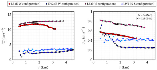
Figure 17.
Uniformity of the mean velocity (left) and the standard deviation (right) of the along-beam component of LW2 and LE during the E-W and N-S configurations, for 10 ms. The scatter plots represent the ensemble averages of N samples of 10 duration.
5. Conclusions
Three synchronized long-range pulsed wind lidars were deployed in the Bjørnafjord, South of Bergen in Norway, in May and June 2016. The purpose of the measurement campaign was to investigate the potential of using lidars to study the wind conditions in the middle of the fjord, where traditional anemometry is not easily deployed. Wind turbulence measurements in such a location are vital to identifying the wind spectral model best suited to estimate the dynamic wind load on a possible future crossing over the 5 wide fjord. During the measurement period, the wind direction was predominantly from north-northwest, with wind velocities up to 18 ms at an altitude of 25 above the mean sea level. The average along-wind turbulence intensity was found to be lower than 0.06 for 8 ms. The normalized wind spectrum for the along-wind component estimated from the lidar data showed a satisfactory agreement with the NORSOK spectrum [10], except for wave-numbers below , where it overestimates the spectral values. If the PSD estimates are not normalized, the NORSOK spectrum overestimates the one estimated from the lidar velocity data, whereas the wind spectrum from the Handbook N400 evaluated using an appropriate roughness length shows a fair agreement with the estimated wind velocity spectrum across the frequency range. The suggested roughness length provided in the Handbook N400 seems, however, to overestimate the one in the middle of a wide fjord in a coastal area.
The along-beam spatial averaging (ABSA) had a significant influence on the estimation of the wind spectrum, down to frequencies around 0.03 , especially because a range gate as large as 75 was used. The measured standard deviation and, therefore, the derived turbulence intensity may be underestimated by up to 16%. Future studies should consider similar wind turbulence measurements with a reduced range gate, where possible. A campaign over extended monitoring time is also a prerequisite to increase the variety of wind conditions within the data set. The ABSA was assumed to play a limited role in the estimation of the coherence. Although this assumption is likely correct for a flow aligned with the scanning beams, further analysis should consider the case where the wind data are retrieved with large yaw angles.
The lateral wind co-coherence was estimated using four measurement volumes, for wind velocities ranging from 6 s to 14 s and a yaw angle up to 10°. The fitted decay coefficients were larger than found in previous studies conducted in fjords, straights or estuaries. The predominance of a stable atmospheric stratification during the measurement period and the relatively low measurement altitude may explain the existence of such a low co-coherence. In this situation, the functional form of the Davenport coherence model may not be well suited to represent the wind co-coherence.
Acknowledgments
The measurements were performed with the support from the Norwegian Public Road Administration. We are indebted to Claus Brian Munk Pedersen and Søren William Lund from the Technical University of Denmark, as well as Jarle Berge from the University of Stavanger, for their assistance during the installation and/or dismantling of the lidar equipment. Finally, we are grateful to Kjeller Vindteknikk for providing the data recorded on the met-mast on the island of Ospøya.
Author Contributions
Jasna B. Jakobsen, Jónas Snæbjörnsson, Jakob Mann, Michael Courtney and Benny Svardal planned the measurement campaign; Guillaume Lea implemented the scanning scenarios, maintained the lidar units and stored the data. Etienne Cheynet analysed the data and wrote the paper, which was also reviewed by the co-authors.
Conflicts of Interest
The authors declare no conflict of interest. The founding sponsors had no role in the design of the study; in the collection, analyses, or interpretation of data; in the writing of the manuscript, and in the decision to publish the results.
Abbreviations
The following abbreviations are used in this manuscript:
| ABSA | Along-beam spatial averaging |
| SA | Sonic anemometer |
| PSD | Power spectral density |
| LOS | Line-Of-Sight |
| N-S | North-South |
| E-W | East-West |
| LE | Lidar East |
| LW1 | Lidar West 1 |
| LW2 | Lidar West 2 |
References
- Newsom, R.; Calhoun, R.; Ligon, D.; Allwine, J. Linearly Organized Turbulence Structures Observed Over a Suburban Area by Dual-Doppler Lidar. Bound. Layer Meteorol. 2008, 127, 111–130. [Google Scholar] [CrossRef]
- Käsler, Y.; Rahm, S.; Simmet, R.; Kühn, M. Wake Measurements of a Multi-MW Wind Turbine with Coherent Long-Range Pulsed Doppler Wind Lidar. J. Atmos. Ocean. Technol. 2010, 27, 1529–1532. [Google Scholar] [CrossRef]
- Cheynet, E.; Jakobsen, J.B.; Snæbjörnsson, J.; Reuder, J.; Kumer, V.; Svardal, B. Assessing the potential of a commercial pulsed lidar for wind characterisation at a bridge site. J. Wind Eng. Ind. Aerodyn. 2017, 161, 17–26. [Google Scholar] [CrossRef]
- Vasiljevic, N.; Courtney, M.; Diaz, A.; Lea, G.; Vignaroli, A. Measuring offshore winds from onshore—One lidar or two? In Proceedings of the EWEA Offshore 2015 Conference, Copenhagen, Denmark, 10–12 March 2015. [Google Scholar]
- Berg, J.; Vasiljevíc, N.; Kelly, M.; Lea, G.; Courtney, M. Addressing Spatial Variability of Surface-Layer Wind with Long-Range WindScanners. J. Atmos. Ocean. Technol. 2015, 32, 518–527. [Google Scholar] [CrossRef]
- Cheynet, E.; Jakobsen, J.B.; Svardal, B.; Reuder, J.; Kumer, V. Wind coherence measurement by a single pulsed Doppler wind lidar. Energy Procedia 2016, 94, 462–477. [Google Scholar] [CrossRef]
- Pauscher, L.; Vasiljevic, N.; Callies, D.; Lea, G.; Mann, J.; Klaas, T.; Hieronimus, J.; Gottschall, J.; Schwesig, A.; Kühn, M.; et al. An Inter-Comparison Study of Multi-and DBS Lidar Measurements in Complex Terrain. Remote Sens. 2016, 8, 782. [Google Scholar] [CrossRef]
- Floors, R.; Peña, A.; Lea, G.; Vasiljević, N.; Simon, E.; Courtney, M. The RUNE experiment—A database of remote-sensing observations of near-shore winds. Remote Sens. 2016, 8, 884. [Google Scholar] [CrossRef]
- The Norwegian Public Roads Administration (NPRA). Bridge Projecting Handbook N400 (in Norwegian); The Norwegian Public Roads Administration: Oslo, Norway, 2015. [Google Scholar]
- NORSOK Standard. Actions and Action Effects; Technical Report, N-003; NORSOK: Lysaker, Norway, 1999. [Google Scholar]
- Lothon, M.; Lenschow, D.; Mayor, S. Coherence and Scale of Vertical Velocity in the Convective Boundary Layer from a Doppler Lidar. Bound. Layer Meteorol. 2006, 121, 521–536. [Google Scholar] [CrossRef]
- Kristensen, L.; Kirkegaard, P.; Mann, J.; Mikkelsen, T.; Nielsen, M.; Sjöholm, M. Spectral Coherence Along a Lidar-Anemometer Beam; Technical Report, Risø-R-1744(EN); Danmarks Tekniske Universitet, Risø Nationallaboratoriet for Bæredygtig Energi: Roskilde, Danmark, 2010. [Google Scholar]
- Davoust, S.; von Terzi, D. Analysis of wind coherence in the longitudinal direction using turbine mounted lidar. J. Phys. Conf. Ser. 2016, 753. [Google Scholar] [CrossRef]
- Cheynet, E.; Jakobsen, J.B.; Snæbjörnsson, J.; Mikkelsen, T.; Sjöholm, M.; Mann, J.; Hansen, P.; Angelou, N.; Svardal, B. Application of short-range dual-Doppler lidars to evaluate the coherence of turbulence. Exp. Fluids 2016, 57, 184. [Google Scholar] [CrossRef]
- Fuertes, F.C.; Iungo, G.V.; Porté-Agel, F. 3D turbulence measurements using three synchronous wind lidars: Validation against sonic anemometry. J. Atmos. Ocean. Technol. 2014, 31, 1549–1556. [Google Scholar] [CrossRef]
- Mann, J.; Cariou, J.P.C.; Parmentier, R.M.; Wagner, R.; Lindelöw, P.; Sjöholm, M.; Enevoldsen, K. Comparison of 3D turbulence measurements using three staring wind lidars and a sonic anemometer. Meteorol. Z. 2009, 18, 135–140. [Google Scholar] [CrossRef]
- Vasiljevic, N.; Lea, G.; Courtney, M.; Cariou, J.P.; Mann, J.; Mikkelsen, T. Long-range WindScanner system. Remote Sens. 2016, 8, 896. [Google Scholar] [CrossRef]
- EN 1991-1-4. Eurocode 1: Actions on Structures—General Actions—Part1-4: Wind Actions; European Committee for Standardization: Brussels, Belgium, 2005. [Google Scholar]
- Teunissen, H. Structure of mean winds and turbulence in the planetary boundary layer over rural terrain. Bound. Layer Meteorol. 1980, 19, 187–221. [Google Scholar] [CrossRef]
- Pearson, R. Mining Imperfect Data: Dealing with Contamination and Incomplete Records; SIAM e-Books; Society for Industrial and Applied Mathematics (SIAM): Philadelphia, PA, USA, 2005. [Google Scholar]
- Panofsky, H.A.; Brier, G.W.; Best, W.H. Some Application of Statistics to Meteorology; Earth and Mineral Sciences Continuing Education, College of Earth and Mineral Sciences, Pennsylvania State University: State College, PA, USA, 1958. [Google Scholar]
- Davenport, A.G. The spectrum of horizontal gustiness near the ground in high winds. Q. J. R. Meteorol. Soc. 1961, 87, 194–211. [Google Scholar] [CrossRef]
- Vickery, B.J. On the reliability of gust loading factors. In Proceedings of Technical Meeting Concerning Wind Loads on Buildings and Structures; Building Science Series 30; National Bureau of Standards: Washington, DC, USA, 1970; pp. 296–312. [Google Scholar]
- Scanlan, R. The action of flexible bridges under wind, II: Buffeting theory. J. Sound Vib. 1975, 60, 201–211. [Google Scholar] [CrossRef]
- Davenport, A.G. The response of Slender, line-like structures to a gusty wind. Proc. Inst. Civ. Eng. 1962, 23, 389–408. [Google Scholar] [CrossRef]
- Solari, G.; Piccardo, G. Probabilistic 3D turbulence modeling for gust buffeting of structures. Probab. Eng. Mech. 2001, 16, 73–86. [Google Scholar] [CrossRef]
- Kristensen, L.; Jensen, N.O. Lateral coherence in isotropic turbulence and in the natural wind. Bound. Layer Meteorol. 1979, 17, 353–373. [Google Scholar] [CrossRef]
- Hjorth-Hansen, E.; Jakobsen, A.; Strømmen, E. Wind buffeting of a rectangular box girder bridge. J. Wind Eng. Ind. Aerodyn. 1992, 42, 1215–1226. [Google Scholar] [CrossRef]
- Krenk, S. Wind field coherence and dynamic wind forces. In IUTAM Symposium on Advances in Nonlinear Stochastic Mechanics; Springer: Dordrecht, The Netherlands, 1996; pp. 269–278. [Google Scholar]
- ESDU 86010. Characteristics of Atmospheric Turbulence Near the Ground Part III: Variations in Space and Time for Strong Winds (Neutral Atmosphere); Technical Report; ESDU: London, UK, 2001. [Google Scholar]
- Andersen, O.J.; Løvseth, J. The Maritime Turbulent Wind Field. Measurements and Models; Final Report for Task 4; Norwegian Institute of Science and Technology: Trondheim, Norway, 1992. [Google Scholar]
- Andersen, O.J.; Løvseth, J. The Frøya database and maritime boundary layer wind description. Mar. Struct. 2006, 19, 173–192. [Google Scholar] [CrossRef]
- Garratt, J. Review of drag coefficients over oceans and continents. Mon. Weather Rev. 1977, 105, 915–929. [Google Scholar] [CrossRef]
- Wiernga, J. Representative roughness parameters for homogeneous terrain. Bound. Layer Meteorol. 1993, 63, 323–363. [Google Scholar] [CrossRef]
- Deardorff, J.W. Dependence of air-sea transfer coefficients on bulk stability. J. Geophys. Res. 1968, 73, 2549–2557. [Google Scholar] [CrossRef]
- Schotanus, P.; Nieuwstadt, F.; De Bruin, H. Temperature measurement with a sonic anemometer and its application to heat and moisture fluxes. Bound. Layer Meteorol. 1983, 26, 81–93. [Google Scholar] [CrossRef]
- Kaimal, J.C.; Gaynor, J.E. Another look at sonic thermometry. Bound. Layer Meteorol. 1991, 56, 401–410. [Google Scholar] [CrossRef]
- Hansen, K.S.; Barthelmie, R.J.; Jensen, L.E.; Sommer, A. The impact of turbulence intensity and atmospheric stability on power deficits due to wind turbine wakes at Horns Rev wind farm. Wind Energy 2012, 15, 183–196. [Google Scholar] [CrossRef]
- Sacré, C.; Delaunay, D. Structure spatiale de la turbulence au cours de vents forts sur differents sites. J. Wind Eng. Ind. Aerodyn. 1992, 41, 295–303. [Google Scholar] [CrossRef]
- Toriumi, R.; Katsuchi, H.; Furuya, N. A study on spatial correlation of natural wind. J. Wind Eng. Ind. Aerodyn. 2000, 87, 203–216. [Google Scholar] [CrossRef]
- Sedefian, L.; Bennett, E. A comparison of turbulence classification schemes. Atmos. Environ. (1967) 1980, 14, 741–750. [Google Scholar] [CrossRef]
- Kareem, A. Wind-induced response analysis of tension leg platforms. J. Struct. Eng. 1985, 111, 37–55. [Google Scholar] [CrossRef]
- Ochi, M.; Shin, V. Wind turbulent spectra for design consideration of offshore structures. In Proceedings of the Offshore Technology Conference, Houston, TX, USA, 2–5 May 1988; pp. 461–467. [Google Scholar]
- Andersen, O.J.; Løvseth, J. Stability modifications of the Frōya wind spectrum. J. Wind Eng. Ind. Aerodyn. 2010, 98, 236–242. [Google Scholar] [CrossRef]
- Mann, J. Engineering Spectra Over Water. In Air-Sea Exchange: Physics, Chemistry and Dynamics; Springer: Dordrecht, The Netherlands, 1999; pp. 437–461. [Google Scholar]
- Angelou, N.; Mann, J.; Sjöholm, M.; Courtney, M. Direct measurement of the spectral transfer function of a laser based anemometer. Rev. Sci. Instrum. 2012, 83. [Google Scholar] [CrossRef] [PubMed]
- Taylor, G.I. The spectrum of turbulence. Proc. R. Soc. Lond. A Math. Phys. Eng. Sci. 1938, 164, 476–490. [Google Scholar] [CrossRef]
- Mizuno, T.; Panofsky, H. The validity of Taylor’s hypothesis in the atmospheric surface layer. Bound. Layer Meteorol. 1975, 9, 375–380. [Google Scholar] [CrossRef]
- Ropelewski, C.F.; Tennekes, H.; Panofsky, H. Horizontal coherence of wind fluctuations. Bound. Layer Meteorol. 1973, 5, 353–363. [Google Scholar] [CrossRef]
- Welch, P.D. The Use of Fast Fourier Transform for the Estimation of Power Spectra: A Method Based on Time Averaging Over Short, Modified Periodograms. IEEE Trans. Audio Electroacoust. 1967, 15, 70–73. [Google Scholar] [CrossRef]
- Kristensen, L.; Kirkegaard, P. Sampling Problems with Spectral Coherence; Risø-R-526; Risø National Laboratory: Roskilde, Denmark, 1986. [Google Scholar]
- Saranyasoontorn, K.; Manuel, L.; Veers, P.S. A comparison of standard coherence models for inflow turbulence with estimates from field measurements. J. Sol. Energy Eng. 2004, 126, 1069–1082. [Google Scholar] [CrossRef]
- Jensen, N.; Hjorth-Hansen, E. Dynamic Excitation of Structures by Wind—Turbulence and Response Measurements at the Sotra Bridge; Technical Report, Report No. STF71 A; Division of Structural Engineering, SINTEF: Trondheim, Norway, 1977. [Google Scholar]
- Cheynet, E. Wind-Induced Vibrations of a Suspension Bridge: A Case Study in Full-Scale. Ph.D. Thesis, University of Stavanger, Stavanger, Norway, 2016. [Google Scholar]
- Bowen, A.J.; Flay, R.G.J.; Panofsky, H.A. Vertical coherence and phase delay between wind components in strong winds below 20 m. Bound. Layer Meteorol. 1983, 26, 313–324. [Google Scholar] [CrossRef]
- Minh, N.N.; Miyata, T.; Yamada, H.; Sanada, Y. Numerical simulation of wind turbulence and buffeting analysis of long-span bridges. J. Wind Eng. Ind. Aerodyn. 1999, 83, 301–315. [Google Scholar] [CrossRef]
- Morfiadakis, E.; Glinou, G.; Koulouvari, M. The suitability of the von Kármán spectrum for the structure of turbulence in a complex terrain wind farm. J. Wind Eng. Ind. Aerodyn. 1996, 62, 237–257. [Google Scholar] [CrossRef]
- Högström, U.; Hunt, J.C.R.; Smedman, A.S. Theory and Measurements for Turbulence Spectra and Variances in the Atmospheric Neutral Surface Layer. Bound. Layer Meteorol. 2002, 103, 101–124. [Google Scholar] [CrossRef]
- Drobinski, P.; Carlotti, P.; Newsom, R.K.; Banta, R.M.; Foster, R.C.; Redelsperger, J.L. The structure of the near-neutral atmospheric surface layer. J. Atmos. Sci. 2004, 61, 699–714. [Google Scholar] [CrossRef]
- Olesen, H.R.; Larsen, S.E.; Højstrup, J. Modelling velocity spectra in the lower part of the planetary boundary layer. Bound. Layer Meteorol. 1984, 29, 285–312. [Google Scholar] [CrossRef]
- Panofsky, H.A.; Mizuno, T. Horizontal coherence and Pasquill’s beta. Bound. Layer Meteorol. 1975, 9, 247–256. [Google Scholar] [CrossRef]
- Hunt, J.C.; Morrison, J.F. Eddy structure in turbulent boundary layers. Eur. J. Mech. B/Fluids 2000, 19, 673–694. [Google Scholar] [CrossRef]
- Hunt, J.; Carlotti, P. Statistical Structure at the Wall of the High Reynolds Number Turbulent Boundary Layer. Flow Turbul. Combust. 2001, 66, 453–475. [Google Scholar] [CrossRef]
- Kristensen, L.; Panofsky, H.A.; Smith, S.D. Lateral coherence of longitudinal wind components in strong winds. Bound. Layer Meteorol. 1981, 21, 199–205. [Google Scholar] [CrossRef]


© 2017 by the authors. Licensee MDPI, Basel, Switzerland. This article is an open access article distributed under the terms and conditions of the Creative Commons Attribution (CC BY) license (http://creativecommons.org/licenses/by/4.0/).