Simulations of the Rotor-Stator-Cavity Flow in Liquid-Floating Rotor Micro Gyroscope

Abstract

When rotating at a high speed in a microscale flow field in confined spaces, rotors are subject to a complex flow due to the joint effect of the centrifugal force, hindering of the stationary cavity and the scale effect. In this paper, a rotor-stator-cavity (RSC) microscale flow field simulation model of liquid-floating rotor micro gyroscopes is built, which can be used to study the flow characteristics of fluids in confined spaces with different Reynolds numbers (Re) and gap-to-diameter ratios. The Reynolds stress model (RSM) is applied to solve the Reynolds averaged Navier–Stokes equation for the distribution laws of the mean flow, turbulence statistics and frictional resistance under different working conditions. The results show that as the Re increases, the rotational boundary layer gradually separates from the stationary boundary layer, and the local Re mainly affects the distribution of velocity at the stationary boundary, while the gap-to-diameter ratio mainly affects the distribution of velocity at the rotational boundary. The Reynolds stress is mainly distributed in boundary layers, and the Reynolds normal stress is slightly greater than the Reynolds shear stress. The turbulence is in the state of plane-strain limit. As the Re increases, the frictional resistance coefficient increases. When Re is within 10⁴, the frictional resistance coefficient increases as the gap-to-diameter ratio decreases, while the frictional resistance coefficient drops to the minimum when the Re exceeds 10⁵ and the gap-to-diameter ratio is 0.027. This study can enable a better understanding of the flow characteristics of microscale RSCs under different working conditions.

1. Introduction

Studies on the flow characteristics of rotor-stator-cavities (RSCs) play an important role in various industrial fields such as turbine machinery [1,2,3], disk drivers [4,5] and chemical stirrers [6,7,8]. Researchers have conducted extensive research on the enclosed viscous flow between rotational and stationary parallel disks by means of simulations, experiments and theoretical analyses. Daliy and Nece [9] took the lead in studying the flow of rotational disks and concluded four basic modes of rotor-stator flows, which are laminar flow with merged boundary layers (Regime I), laminar flow with unmerged boundary layers (Regime II), turbulent flow with merged boundary layers (Regime III) and turbulent flow with unmerged boundary layers (Regime IV). Gauthier et al. [10] studied the generation and spread of unstable disk flows in enclosed cavities through visualization methods and found that unstable fluctuations first appear in the stationary wall boundary layer as the Reynolds number (Re) increases. If Re continues to increase, such fluctuations gradually develop into annular waves and spiral waves that spread continuously from the edge to the center, and eventually develop into areas of turbulence. Schouvelier et al. [11,12] studied the correlation between Re and the gap-to-diameter ratio and the RSC flow field stability by photographing the wave structure and vortex structure in the flow field and mapped the flow fluctuations of disks in enclosed cavities. Watanabe et al. [13,14] carried out simulations and experiments to study the effects of radial slits and the size of such slits on the fluid structure in cavities. Serre et al. [15], through 3D direct numerical simulation, analyzed the relationship between the spatial structure and time of flows in annular and cylindrical cavities at different curvature and aspect ratios. Hara et al. [16] selected five disks of different radii to study the effects of the size of the radial gap and Re on the flow structure and drew the statistical map of morphological change nodes of the Taylor vortex and fluctuant vortex.

Nowadays, miniaturisation and portability of instruments and equipment have become a trend. The widespread use of MEMS technology has driven the market’s demand for micro gyroscopes [17,18,19], micro disks [5] and other micro rotating devices. As the devices get smaller, frictional resistance will cause not only higher energy consumption but also poorer performance and shorter service lives, which hinders the application of micro devices. Heating and increased power consumption caused by solid–liquid frictional resistance [20,21] are especially significant in liquid-floating micro gyroscopes. However, the changes of fluid flow, temperature distribution, torque and driving power between disks at micro scale have not been fully studied [11,12,13,14,22]. Therefore, it is necessary to investigate the flows of microscale rotational disks.

Three methods are mainly used to simulate turbulent flow, direct numerical simulation (DNS), large-eddy simulation (LES) and Reynolds-averaged Navier–Stokes (RANS). DNS and LES are regarded as the most accurate and trustworthy in unsteady high-Reynolds wall flows, but DNS is too expensive to be applied in complex project and LES just solve the turbulent scales of greater intensity. Due to its modest computing requirements, RANS has been the most popular method for industrial CFD applications over the past few decades, although errors introduced by modeling all turbulence scales would reduce predictive power. RANS decomposes the instantaneous motion that satisfies the dynamic equation into average motion and fluctuation motion, where the fluctuation item is represented by Reynolds stress. It solves only for the averaged quantities while the effect of all the scales of instantaneous turbulent motion is modelled by a turbulence model [23,24]. Among all the turbulence models, the RSM is the most consistent with the physical understanding of the RANS, considering the anisotropy of eddy viscosity. It is suitable for rotating flow, curved pipe flow, etc. [25].

In this paper, an RSC microscale flow field simulation model of liquid-floating rotor micro gyroscopes is established to calculate the flow field distribution at different Re numbers and gap-to-diameter ratios with the Reynolds stress model (RSM). The mean flow, turbulence statistics and frictional resistance coefficient in axial slits and the distribution law of the vortex structure in radial slits have been attained, which provides support for the design of liquid-floating rotor micro gyroscopes. Simultaneously, this work has great significance for the design and parameter setting of the devices with microscale RSC flow fields.

2. Model Parameters and Numerical Method

Figure 1 shows the section of the flow field in the r-z plane. The origin of the coordinate axis is at the center of the upper face of the disk. r represents radial distance from the origin. The radius and thickness of the disk are recorded as R_d and H_d, and those of the cavity as R_c and H_c, respectively. The size of the upper axial slit H_u is the same as that of the lower axial slit H_l. The disk rotates at the angular speed of ω, and the liquid in the cavity is water. At 20 °C, the kinetic viscosity coefficient v of water is 1.007 × 10⁻⁶ m²/s, and Re, local Reynolds number Re_l and the gap-to-diameter ratio G are calculated in Equations (1)–(3).

$$Re=\omega R_d^2/v,$$

(1)

$${Re}_l=\omega r^2/v,$$

(2)

$$G=H_u/R_d.$$

(3)

For the modelling in simulation, H_u is set as 100 μm, 200 μm and 300 μm, and other parameters are as shown in

Table 1. Model parameters.

Rd (mm)	Hd (mm)	Rc (mm)
7.5	2	8

.

The flow field model in this study is affected jointly by the rotational state of the rotor, the scale effect and the wall effect of the flow field, with complex flow characteristics and harsh requirements especially for the calculation of the turbulence. The RSM model can accurately simulate the flows in RSCs, especially at the points near the boundary of the disk where most of the turbulence is. It can describe in detail the near-wall turbulence without being affected by any hypothesis of eddy viscosity [26].

ANSYS Fluent was used for simulation. First, the 3D model was built. The radial scale of the simulated flow field is much larger than the axial scale, so the model was divided into upper and lower end caps, upper and lower ring domains, and cylindrical areas. Second, the grid independence verification had been done to ensure the efficiency and accuracy of the solution calculation. Each area was meshed separately with structured grid. The grids near the rotor wall and the cavity shell wall were refined. The grid orthogonality quality was used for evaluation. The grid quality distribution was concentrated at 0.8, indicating that the grid quality was better. Third, convenience conditions and initial conditions were set. The upper and lower end surfaces and side walls of the rotor were set as the rotation boundary and the rotation speed was set to 300 rpm, 1200 rpm, 3000 rpm, 6000 rpm, 12,000 rpm, etc. All the walls of the cavity shell were set as the static boundary. All walls were set as no-slip boundary conditions. The liquid in the model was set to be water at 20 °C. Fourth, the parameters of solver were set. Pressure, momentum, turbulent kinetic energy and turbulent diffusion rate adopted the standard, the second-order upwind, the first-order upwind and the first-order upwind, respectively. After discretization, the SIMPLE algorithm was used to solve the pressure coupling equation. The equations solved by Fluent are non-linear, and only by controlling the variable value in each iteration can the divergence caused by large difference be effectively avoided. It is regulated by the relaxation factor. After testing, when the relaxation factor of each calculation parameter was set to

Table 2. Values of relaxation factor for different parameters.

Parameter	Pressure	Body Force	Momentum	Turbulent Kinetic Energy
Relaxation Factor	0.3	0.5	0.4	0.4

, the calculation was easy to converge. Last, iterative calculations were performed. The convergence standard of the residual value of each variable was set to 10⁻⁶. In addition, the velocity of a certain point in the model was selected as a reference. When it reached stability, the calculation result was considered to have converged.

In the subsequent study, all variables are normalised in the following way: $Z^{*}=z/H_u$, $r^{*}=r/R_d$, $V_i^{*}=V_i/\left(\omega \times r\right)$, $R_{ij}^{*}=v_i{v}_j/{\left(\omega \times r\right)}^2$, where i and j are any direction vector of the cylindrical-coordinate system r, θ and z, Z* and r* are the axial coordinate and circumferential coordinate after normalisation, $V_{\theta }^{*}$ and $V_r^{*}$ are the circumferential velocity and radial velocity after normalisation, v_i and v_j are the fluctuating velocity, $R_{ij}^{*}\left(i\ne j\right)$ is the Reynolds shear stress, $R_{ij}^{*}\left(i=j\right)$ is the Reynolds normal stress.

3. Results and Discussion

3.1. Mean Flow of the Axial Gap

Figure 2 illustrates the distribution of the circumferential velocity $V_{\theta }^{*}$ and the radial velocity $V_r^{*}$ along the z-axis when Re is 7.02 × 10⁴ and the gap-to-diameter ratio is 0.027. The axial velocity of the fluid at positions other than those around the rotor and near the edge of the lateral wall of the cavity is 0, which, therefore, is not given here. The radius r* ranges from 0.067 to 0.967. Z* is 0 at the rotational wall, and Z* is 1 at the stationary wall. The velocity gradually decreases from the rotational boundary to the stationary boundary layer due to the non-slip boundary condition. The velocity gradient first decreases and then increases, and it changes more significantly at the position of a greater r*. When Z* < 0.1 (z < 20 μm), the circumferential velocity changes almost in the same way, and then the separation gradually occurs. According to the above results, there is no core region with a velocity gradient of 0, but the velocity gradient tends to 0 as the Re_l increases. The centrifugal force generated by the rotating motion of the rotor causes the fluid near the rotational wall to be thrown out along the radius, so the radial velocity is a positive value. Following the law of conservation of mass, the fluid flows inward along the stationary wall, causing the radial velocity of the fluid near the stationary wall to have a negative value. As a result, the entire radial velocity is in an S-shaped distribution along the z-axis. Near the rotational wall, the position of the V_r* extremum remains almost unchanged, which is near Z* = 0.1, while for the fluid near the stationary wall, the position of the V_r* extremum increases as r* increases, which is offset to the stationary wall. According to the research by Daliy and Nece [9], the flow at this point is Regime II, which is the laminar flow with unmerged boundary layers. The boundary layer near the stationary wall is called the Ekman boundary layer [27], the thickness of which decreases as r* increases, while the boundary layer near the rotational wall is called the Bödewadt boundary layer [27], the thickness of which remains almost unchanged.

Figure 3 displays the distribution curves of the circumferential velocity and radial velocity along the z-axis with the change of Re (1.75 × 10³ ≤ Re ≤ 7.02 × 10⁴). The axial velocity V_z* is still extremely low under this condition, so it is ignored. When Re = 7.02 × 10³ (at 1200 rpm rotational speed), the circumferential velocity is in a linear distribution along the z-axis. With the increase in Re, the flow of the fluid in the axial slit changes from the torsional Couette flow with a merged boundary layer to the laminar Batchelor flow with unmerged boundary layers, that is, it changes gradually from Regime I to Regime II [9]. When Re ≥ 1.75 × 10⁴ (at 3000 rpm rotational speed), the boundary layer gradually separates, and the separation becomes more significant as Re increases. The radial velocity V_r*, as a whole, retains its S shape, but its extremum increases as Re increases, and its position goes closer to the wall, with almost the same change law within the range of 0.4 ≤ Z* ≤ 0.6.

Figure 4 shows the distribution curves of the circumferential velocity V_θ* and the radial velocity V_r* along the z-axis with the change of the gap-to-diameter ratio G. Under all three working conditions, the motion of the fluid is in Regime II, the laminar flow with unmerged boundary layers. The circumferential velocity V_θ*, when near the stationary wall (Z* > 0.7), has almost the same change law, which is irrelevant to the gap-to-diameter ratio, but near the rotational wall, its gradient increases as the gap-to-diameter ratio increases. However, under all working conditions, the radial velocity V_r* is in an S-shaped distribution, and its extremum increases as the gap-to-diameter ratio increases, but its position along the axis is irrelevant to the gap-to-diameter ratio. Its extremum near the rotational wall is near Z* = 0.12, and the same near the stationary wall is near Z* = 0.85.

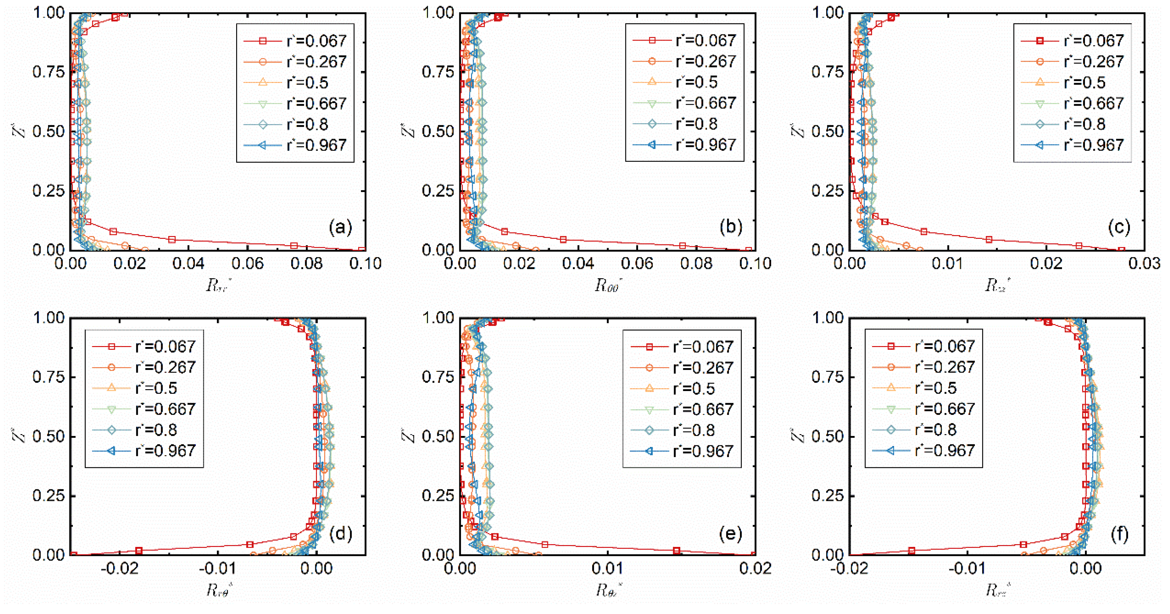
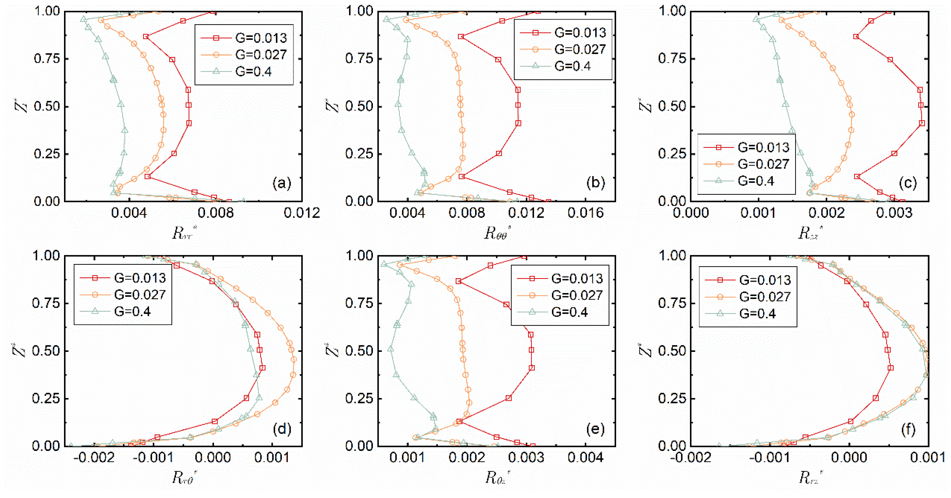
3.2. Turbulence Statistics in the Axial Gap

The distribution curves along the z-axis of the six components of the Reynolds stress tensor, R_rr*, R_θθ*, R_zz*, R_rθ*, R_θz* and R_rz*, at the given Re = 7.02 × 10⁴ and gap-to-diameter ratio G = 0.027 are shown in Figure 5. It can be seen from the figure that the Reynolds stresses of the turbulence are mainly concentrated near the boundary layer. The Reynolds stresses are all 0 in the central flow field area when r* = 0.067, while almost all of them have a positive value at the other radii monitored. With the increase in r*, the local Reynolds number Re_l increases, the Reynolds stress slightly increases and the normal stress is higher than the shear stress.

Figure 6 shows the distribution curves of the six components of the Reynolds stress tensor along the z-axis at different Re when the gap-to-diameter ratio G = 0.027 and r* = 0.8. It can be observed that the Re gradually decreases from the red line to the blue line, and the Reynolds stresses are of an approximately symmetric distribution with Z* = 0.5 as the axis of symmetry. When Re ≤ 7.02 × 10³, the Reynolds normal stress decreases and then increases from the stationary boundary layer to the rotational boundary layer and has a lateral U-shaped distribution, while it is in an Σ-shaped distribution along the z-axis when Re ≥ 1.75 × 10⁴. The Reynolds shear stress changes similarly near the rotational boundary layer (0 ≤ Z* < 0.1) and the stationary boundary layer (0.85 < Z* ≤ 1) at different Re and increases as Re increases in the central area of the axial slit (0.1 ≤ Z* ≤ 0.85), but is significantly lower than the normal stress.

Figure 7 illustrates the distribution curves of the six components of the Reynolds stress tensor along the z-axis at different gap-to-diameter ratios when Re = 7.02 × 10⁴ and r* = 0.8. The normal stresses are in an Σ-shaped distribution and decrease as the gap-to-diameter ratio increases, but the three shear stresses have no such change. The Reynolds shear stress R_rθ* and R_rz* have negative values near the wall, and positive values near the central area of the slit, which is related to the centrifugal force and conservation of mass.

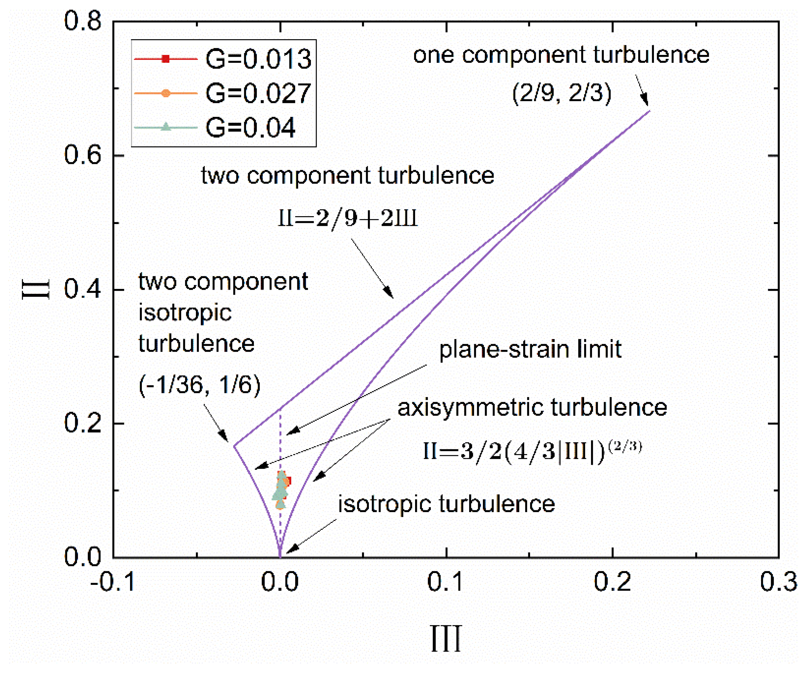
3.3. Anisotropy Analysis of Turbulence in the Axial Gap

The anisotropy invariant map (AIM) is an important method proposed by Lumley [28] to describe the morphology and structure of turbulence. Figure 8 shows a triangle bounded by three curves and their corresponding equations. The three purple curves indicate the limiting boundaries of the morphology of turbulent fluctuations, which is called the Lumley triangle. Fluctuations of turbulence can be described by analyzing the anisotropy tensor a_ij in Equations (4) and (5).

$$a_{ij}=\stackrel{-}{u_i^{\prime }{u}_j^{\prime }}/2k-{\delta }_{ij}/3.$$

(4)

where $u_i^{\prime }$ is the instant velocity fluctuation along the i direction, $k=\stackrel{-}{u_n^{\prime }{u}_n^{\prime }}/2$ is the turbulent kinetic energy, δ_ij is the Kronecker delta function, and the tensor a_ij has three scalar invariants:

$$\mathrm{I}=a_{ij}=0,\mathrm{I}\mathrm{I}=a_{ij}{a}_{ji},\mathrm{I}\mathrm{I}\mathrm{I}=a_{ij}{a}_{jk}{a}_{ki}.$$

(5)

Through calculation, the distributions of the AIMs at different gap-to-diameter ratios when Re = 7.02 × 10⁴ and r* = 0.8 are shown by the red, blue and green spots in Figure 8. Under all three working conditions, the scalar III is approximately 0, so the turbulence is in the state of the plane-strain limit [29].

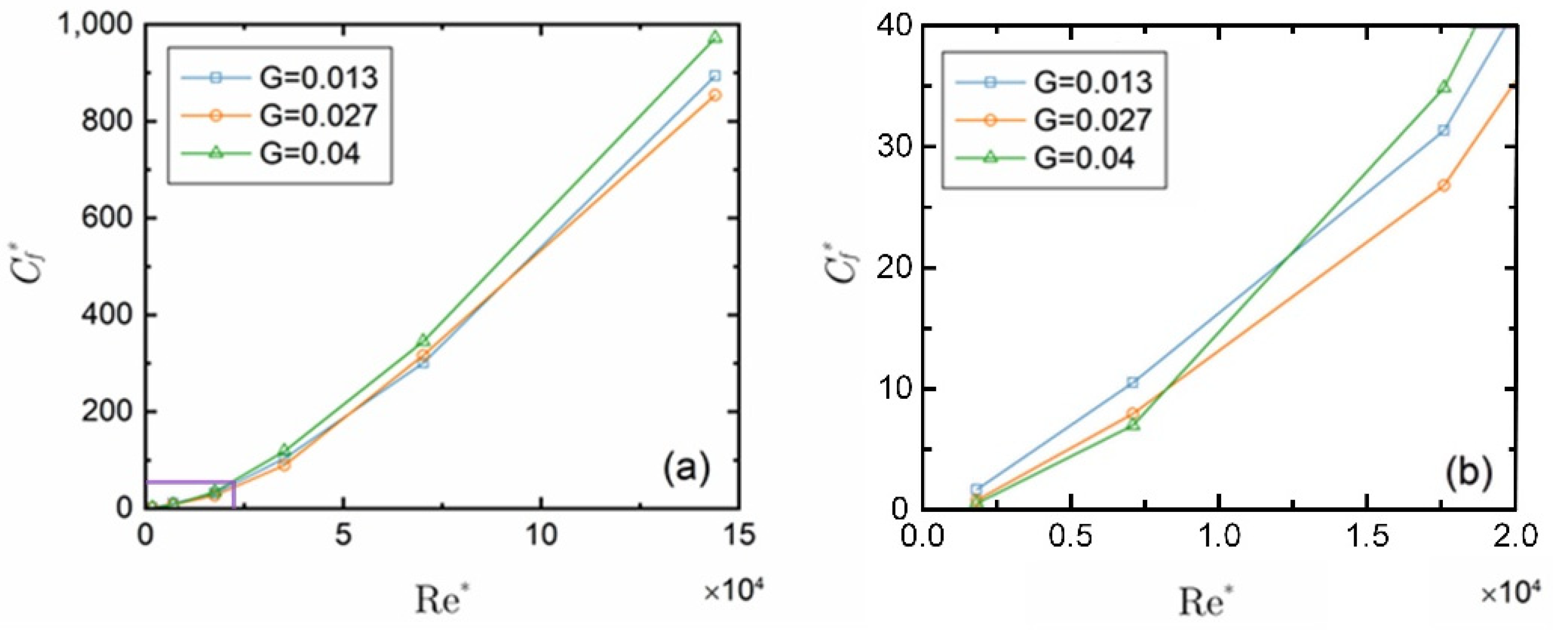
3.4. Skin Friction Coefficient

Figure 9 displays the curves of the mean value of the rotor’s skin friction coefficient C_f* (including the upper and lower faces and the cylindrical face of the rotor) with Re at three gap-to-diameter ratios, where (b) is the partial enlarged view of the area in the purple box in (a). The skin friction coefficient increases with Re under all three working conditions. When Re < 10⁴, the C_f* decreases as the gap-to-diameter ratio G increases, as shown in Figure 9b, and as Re continues to increase, the C_f* at G = 0.04 gradually becomes the maximum, while the C_f* at G = 0.027 becomes the minimum value when Re is greater than 9.6 × 10⁴. The main reason may be that at a low Re, the friction coefficients of the end faces and the cylindrical face are in the same order of magnitude, and that at a greater gap-to-diameter ratio they are in a smaller velocity gradient, making the C_f* decrease as the gap-to-diameter ratio increases. When Re increases, the stress in the radial slit changes more significantly at a greater gap-to-diameter ratio, causing the friction coefficient of the cylindrical face to significantly increase and the velocity of such increase to be greater than that of the friction coefficient of the end faces, making the C_f* reach its maximum when the gap-to-diameter ratio G = 0.04. Moreover, as Re increases, the velocity gradient changes more significantly at a smaller gap-to-diameter ratio, so C_f* at G = 0.013 gradually exceeds that at G = 0.027. For the liquid-floating rotor micro gyroscope in this work, the higher the rotating speed, the more significant the gyroscopic effect and the greater the frictional resistance, resulting in noticeable power consumption and heating. Under the three working conditions in this study, a gap-to-diameter ratio G of 0.027, i.e., an axial slit of 200 μm, is the optimal choice.

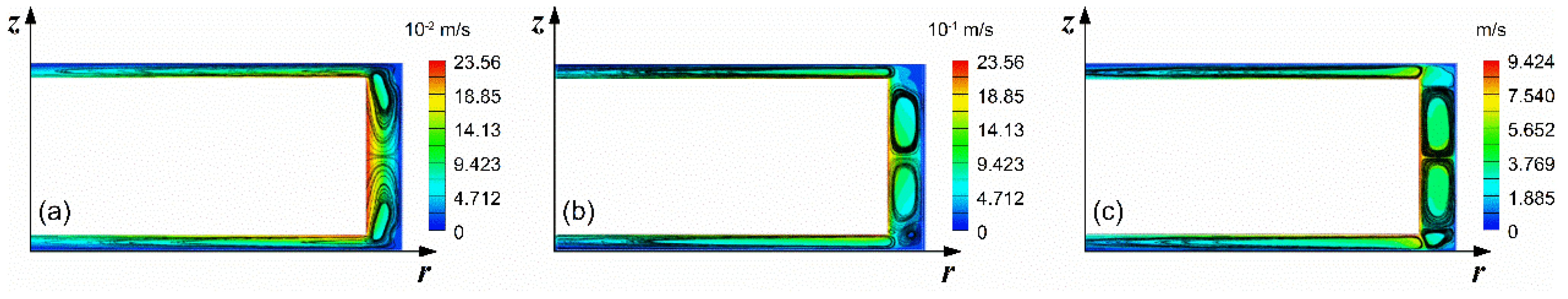
3.5. Flow Vortex Structure Distribution in the Radial Gap

An increase in Re may change the flow distribution of the flow field in the axial gap, and also affect the vortex structure in the radial gap. The model is divided along the r-z plane to observe the distribution of the Taylor vortex on the section, as shown in Figure 10. At a low Re, the Taylor vortex in the radial gap is integrated with the circulating flow in the axial gap, and as Re increases, they are gradually separated from each other, because the viscosity force decreases, and the laminar flow becomes unstable. When Re increases to 7.02 × 10⁴, four independent areas of Taylor turbulence appear in the axial gap, which are of an approximately symmetric distribution.

The cloud image of the intensity distribution of the spiral vortices on different faces in the θ-z plane is shown in Figure 11. The spiral vortex near the cylindrical face of the rotor is significantly more intense than that near the lateral wall of the cavity. At a low Re, most of the spiral vortices are near the axial slit of the rotor. As Re increases, the range of the spiral vortices gradually expands and covers the center of the flow field. When Re increases to 7.02 × 10⁴, the spiral vortices fluctuate approximately periodically, and gradually fill the entire flow field.

4. Conclusions

In this paper, an RSC microscale flow field simulation model of liquid-floating rotor micro gyroscopes is built to calculate the flow field distribution at different values of Re and gap-to-diameter ratios with the RSM. The mean flow, turbulence statistics, anisotropic distribution of turbulence and the change laws of the flow vortex structure and frictional resistance coefficient in the radial gap have been attained.

(1)

Along the z-axis, the circumferential velocity gradually develops from a linear distribution to a non-linear distribution with separated boundary layers, i.e., from a torsional Couette flow to a Batchelor flow, as Re increases. The greater the Re is, the more the velocity gradient in the middle part tends to 0. The local Re (Re_l) and the gap-to-diameter ratio (G) affect the boundary layers in different ways. The former mainly affects the velocity distribution near the stationary boundary, and an increase in it causes an increase in the velocity gradient. The latter mainly affects the velocity distribution near the rotational wall, and an increase in it causes a decrease in the velocity gradient. The radial velocity is in an S-shaped distribution under all three working conditions. Due to the centrifugal force, the fluid near the rotational wall flows outward along the radius, while that near the stationary wall flows inward along the radius to supplement the former. Both Re and the gap-to-diameter ratio affect the extremum of the radial velocity and its position along the z-axis. Compared with the circumferential velocity and the radial velocity, the axial velocity is quite small, nearly 0 in the axial slit.

(2)

The Reynolds stresses are mainly in an Σ-shaped and lateral U-shaped distribution at different values of Re and gap-to-diameter ratios. Most of the areas of turbulence are near the stationary boundary layer and the rotational boundary layer. When Re > 10⁴, Re has little effect on the distribution of the Reynolds stresses along the z-axis. As the gap-to-diameter ratio increases, the maximum of the Reynolds normal stress increases, and the Reynolds shear stress has no obvious law. According to the analysis results of the anisotropy invariants of the turbulence under different working conditions, the turbulence in this work is in the state of the plane-strain limit.

(3)

The skin friction coefficient increases as Re increases. When Re < 10⁴, the greater the gap-to-diameter ratio, the smaller the friction resistance coefficient. If Re > 10⁴, it increases the most slowly with the gap-to-diameter ratio G = 0.027. When Re increases to 9.6 × 10⁴, the skin friction coefficient is smaller with G = 0.027 than that with G = 0.04 and 0.013.

(4)

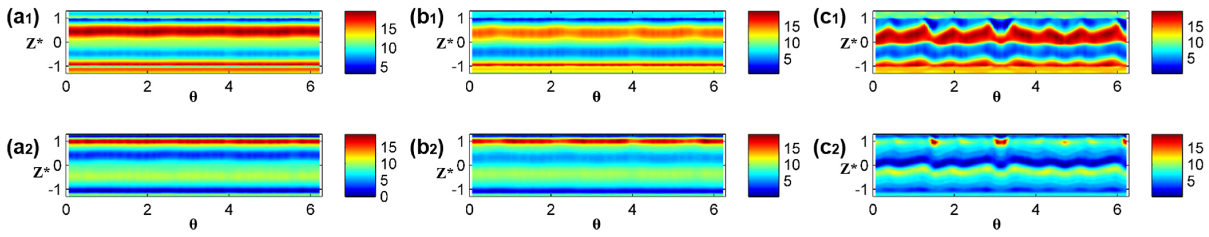
As Re increases, the flow vortex structure in the radial gap gradually separates. When Re increases from 1.75 × 10³ to 7.02 × 10⁴, the vortex structure in the radial gap gradually separates from the circulating flow in the axial gap, and eventually forms four independent vortices in the radial gap. An increase in Re causes the range of spiral vortices to gradually expand from the cylindrical face of the rotor to the lateral wall of the cavity. When Re ≥ 7.02 × 10⁴, periodic fluctuations appear in spiral vortices in the radial gap.

References

1. Poncet, S.; Chauve, M.P.; Schiestel, R. Batchelor versus Stewartson flow structures in a rotor-stator cavity with throughflow. Phys. Fluids 2005, 17, 075110. [Google Scholar] [CrossRef]
2. Wu, S.-C. A PIV study of co-rotating disks flow in a fixed cylindrical enclosure. Exp. Therm. Fluid Sci. 2009, 33, 875–882. [Google Scholar] [CrossRef]
3. Harmand, S.; Pellé, J.; Poncet, S.; Shevchuk, I.V. Review of fluid flow and convective heat transfer within rotating disk cavities with impinging jet. Int. J. Therm. Sci. 2013, 67, 1–30. [Google Scholar] [CrossRef] [Green Version]
4. Shirai, K.; Yaguchi, Y.; Büttner, L.; Czarske, J.; Obi, S. Highly spatially resolving laser Doppler velocity measurements of the tip clearance flow inside a hard disk drive model. Exp. Fluids 2011, 50, 573–586. [Google Scholar] [CrossRef]
5. Kang, C.I.; Baek, S.E.; Shim, J.S. A new seek servo controller for minimizing power consumption in micro hard disk drives. IEEE Trans. Magn. 2004, 40, 3127–3129. [Google Scholar] [CrossRef]
6. Meeuwse, M.; Van der Schaaf, J.; Kuster BF, M.; Schouten, J.C. Gas–liquid mass transfer in a rotor–stator spinning disc reactor. Chem. Eng. Sci. 2010, 65, 466–471. [Google Scholar] [CrossRef]
7. Meeuwse, M.; Van Der Schaaf, J.; Schouten, J.C. Multistage rotor-stator spinning disc reactor. Aiche J. 2012, 58, 247–255. [Google Scholar] [CrossRef]
8. Visscher, F.; Van Der Schaaf, J.; De Croon, M.H.; Schouten, J.C. Liquid–liquid mass transfer in a rotor–stator spinning disc reactor. Chem. Eng. Sci. 2012, 185, 267–273. [Google Scholar] [CrossRef]
9. Daily, J.W.; Nece, R.E. Chamber dimension effects on induced flow and frictional resistance of enclosed rotating disks. J. Fluids Eng. 1960, 82, 217. [Google Scholar] [CrossRef]
10. Gauthier, G.; Gondret, P.; Rabaud, M.J. Axisymmetric propagating vortices in the flow between a stationary and a rotating disk enclosed by a cylinder. J. Fluid Mech. 1999, 386, 105–126. [Google Scholar] [CrossRef]
11. Schouveiler, L.; Le Gal, P.; Chauve, M.P. Stability of a traveling roll system in a rotating disk flow. Phys. Fluids 1998, 10, 2695–2697. [Google Scholar] [CrossRef]
12. Schouveiler, L.; Le Gal, P.; Chauve, M.P. Instabilities of the flow between a rotating and a stationary disk. J. Fluid Mech. 2001, 443, 329–350. [Google Scholar] [CrossRef]
13. Watanabe, T.; Furukawa, H. The effect of rim-shroud gap on the spiral rolls formed around a rotating disk. Phys. Fluids 2010, 22, 114107. [Google Scholar] [CrossRef]
14. Watanabe, T.; Furukawa, H. Flows around rotating disks with and without rim-shroud gap. Exp. Fluids 2010, 48, 631–636. [Google Scholar] [CrossRef]
15. Serre, E.; Del Arco, E.C.; Bontoux, P. Annular and spiral patterns in flows between rotating and stationary discs. J. Fluid Mech. 2001, 434, 65–100. [Google Scholar] [CrossRef]
16. Hara, S.; Watanabe, T.; Furukawa, H.; Endo, S. Effects of a radial gap on vortical flow structures around a rotating disk in a cylindrical casing. J. Vis. 2015, 18, 501–510. [Google Scholar] [CrossRef]
17. Zhang, H.F.; Zhang, X.S.; Liu, X.W.; Liang, Y.C.; Weng, R. Edge Effect on Viscous Drag of the Rotor in Liquid Floating Rotational Micro-Gyroscope. In Key Engineering Materials; Trans Tech Publications Ltd.: Bach SZ, Switzerland, 2013; Volume 562, pp. 286–291. [Google Scholar]
18. Wang, C.; Tang, F.; Hao, P.F.; Li, Q.; Wang, X.H. Experimental study on the drag reduction effect of a rotating superhydrophobic surface in micro gap flow field. Microsyst. Technol. 2017, 23, 3033–3040. [Google Scholar] [CrossRef]
19. Han, F.T.; Liu, Y.F.; Wang, L.; Ma, G.Y. Micromachined electrostatically suspended gyroscope with a spinning ring-shaped rotor. J. Micromech. Microeng. 2012, 22, 105032. [Google Scholar] [CrossRef]
20. Yin, L.; Zhang, H.; Weng, R.; Wu, Z.; Liu, X. Fabrication and drag reduction of the superoleophobic surface on a rotational gyroscope. Surf. Eng. 2018, 34, 165–171. [Google Scholar] [CrossRef]
21. Chen, D.; Liu, X.; Zhang, H.; Li, H.; Weng, R.; Li, L.; Zhang, Z. Friction reduction for a rotational gyroscope with mechanical support by fabrication of a biomimetic superhydrophobic surface on a ball-disk shaped rotor and the application of a water film bearing. Micromachines 2017, 8, 223. [Google Scholar] [CrossRef] [Green Version]
22. Jiji, L.M.; Ganatos, P. Microscale flow and heat transfer between rotating disks. Int. J. Heat Fluid Flow 2010, 31, 702–710. [Google Scholar] [CrossRef]
23. De Vanna, F.; Baldan, G.; Picano, F.; Benini, E. Effect of convective schemes in wall-resolved and wall-modeled LES of compressible wall turbulence. Comput. Fluids 2023, 250, 105710. [Google Scholar] [CrossRef]
24. Yang, Z.Y. Large-eddy simulation: Past, present and the future. Chin. J. Aeronaut. 2015, 28, 11–24. [Google Scholar]
25. Li, P.; Xu, M.; Wang, F. Proficient in CFD Engineering Simulation and Case Practice: Fluent Gambit Icem CFD Tecplot; Post & Telecom Press: Beijing, China, 2011. [Google Scholar]
26. Haddadi, S.; Poncet, S. Turbulence Modeling of Torsional Couette Flows. Int. J. Rotating Mach. 2008, 2008. [Google Scholar] [CrossRef] [Green Version]
27. Launder, B.; Poncet, S.; Serre, E. Laminar, transitional, and turbulent flows in rotor-stator cavities. Annu. Rev. Fluid Mech. 2010, 42, 229–248. [Google Scholar] [CrossRef] [Green Version]
28. Lumley, J.L.; Newman, G.R. The return to isotropy of homogeneous turbulence. J. Fluid Mech. 1977, 82, 161–178. [Google Scholar] [CrossRef] [Green Version]
29. Simonsen, A.; Krogstad, P.Å. Turbulent stress invariant analysis: Clarification of existing terminology. Phys. Fluids 2005, 17, 088103. [Google Scholar] [CrossRef] [Green Version]
Figure 1. Schematic diagram of the gemetry in the r-z plane.
Micromachines 14 00793 g001
Figure 2. Distribution curve of mean velocity along the z-axis when Re = 7.02 × 10⁴ (12,000 rpm) and G = 0.027. (a) Circumferential velocity; (b) Radial velocity.
Micromachines 14 00793 g002
Figure 3. Distribution curve of the velocity component along the z-axis when r* = 0.8 and G = 0.027. (a) Circumferential velocity; (b) Radial velocity.
Micromachines 14 00793 g003
Figure 4. Distribution curve of the velocity component along the axis-z when r* = 0.8 and Re = 7.02 × 10⁴. (a) Circumferential velocity; (b) Radial velocity.
Micromachines 14 00793 g004
Figure 5. Change of the six components of the Reynolds stress tensor (af) with the radial position r* when Re = 7.02 × 10⁴ and G = 0.027.
Micromachines 14 00793 g005
Figure 6. Change of the six components of the Reynolds stress tensor (af) with Re when G = 0.02 and r* = 0.8.
Micromachines 14 00793 g006
Figure 7. Change of the six components of the Reynolds stress tensor (af) with the gap-to-diameter ratio G when Re = 7.02 × 10⁴ and r* = 0.8.
Micromachines 14 00793 g007
Figure 8. The anisotropy invariant map.
Micromachines 14 00793 g008
Figure 9. Change of the skin friction coefficient of the rotor with Re: (a) Overall view; (b) Partial enlarged view.
Micromachines 14 00793 g009
Figure 10. Distribution of the Taylor turbulence at different Re. (a) Re = 1.75 × 10³; (b) Re = 1.75 × 10⁴; (c) Re = 7.02 × 10⁴.
Micromachines 14 00793 g010
Figure 11. Cloud image of intensity distribution of spiral vortices. (a1,b1,c1) are 10 μm to the lateral wall of the rotor; (a2,b2,c2) are 10 μm to the lateral wall of the cavity; (a) Re = 1.75 × 10³; (b) Re = 1.75 × 10⁴; (c) Re = 7.02 × 10⁴.
Micromachines 14 00793 g011