
Universal Markers Unveil Metastatic Cancerous Cross-Sections at Nanoscale

 , , ,
, , ,  ,
,  ,
,  and
and 
Abstract
:Simple Summary
Abstract
1. Introduction
2. Materials and Methods
2.1. Histological Tissue Preparation
2.2. AFM Image Analysis
2.3. AFM Image Mathematical Analysis
3. Results
4. Discussion
5. Conclusions
Author Contributions
Funding
Institutional Review Board Statement
Informed Consent Statement
Data Availability Statement
Conflicts of Interest
Abbreviations
| FD | Fractal dimension |
| M | Metastatic cross-sections |
| NM | Non-metastatic cross-sections |
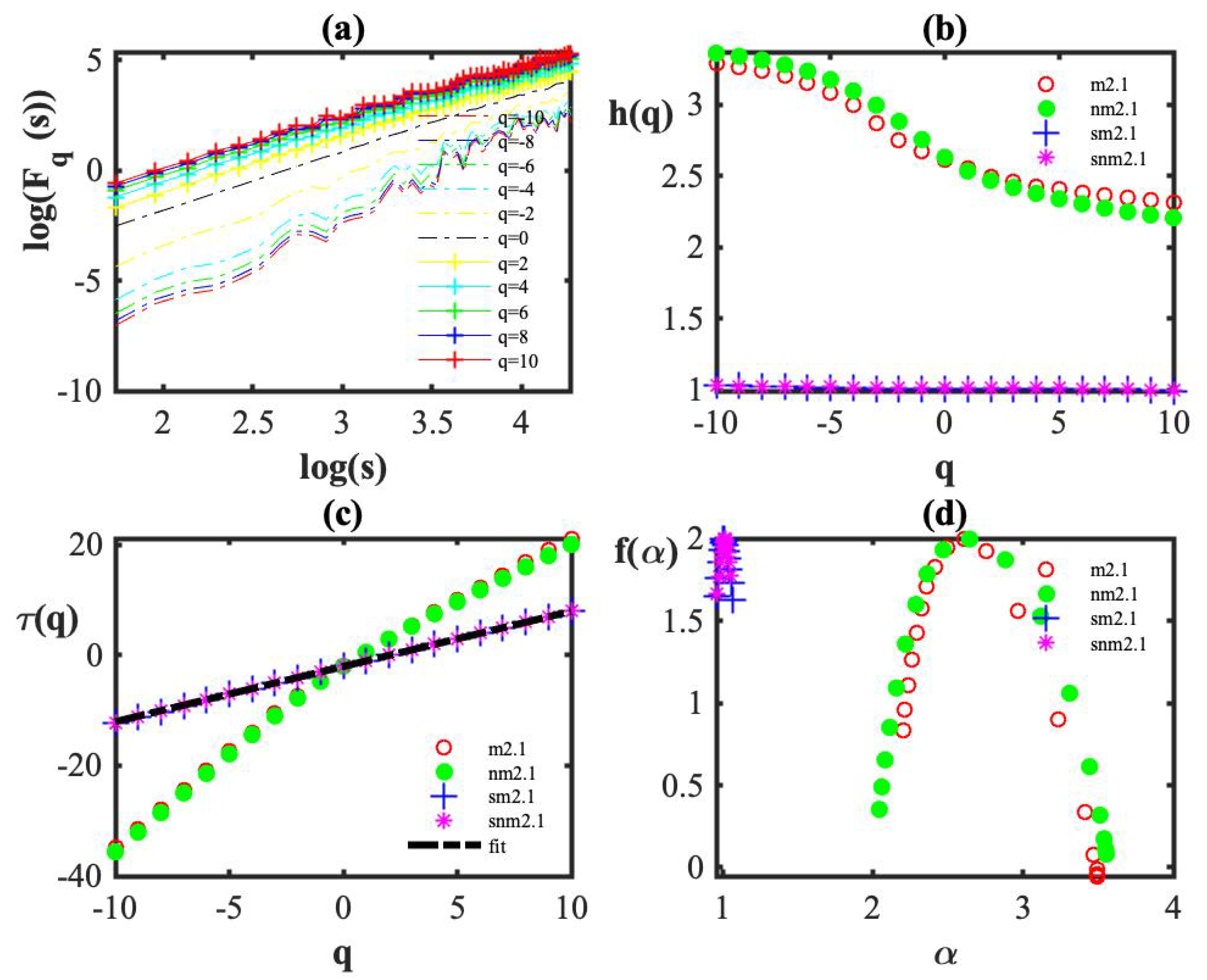
| 2D MF-DFA | Two-dimensional multifractal detrended fluctuation analysis |
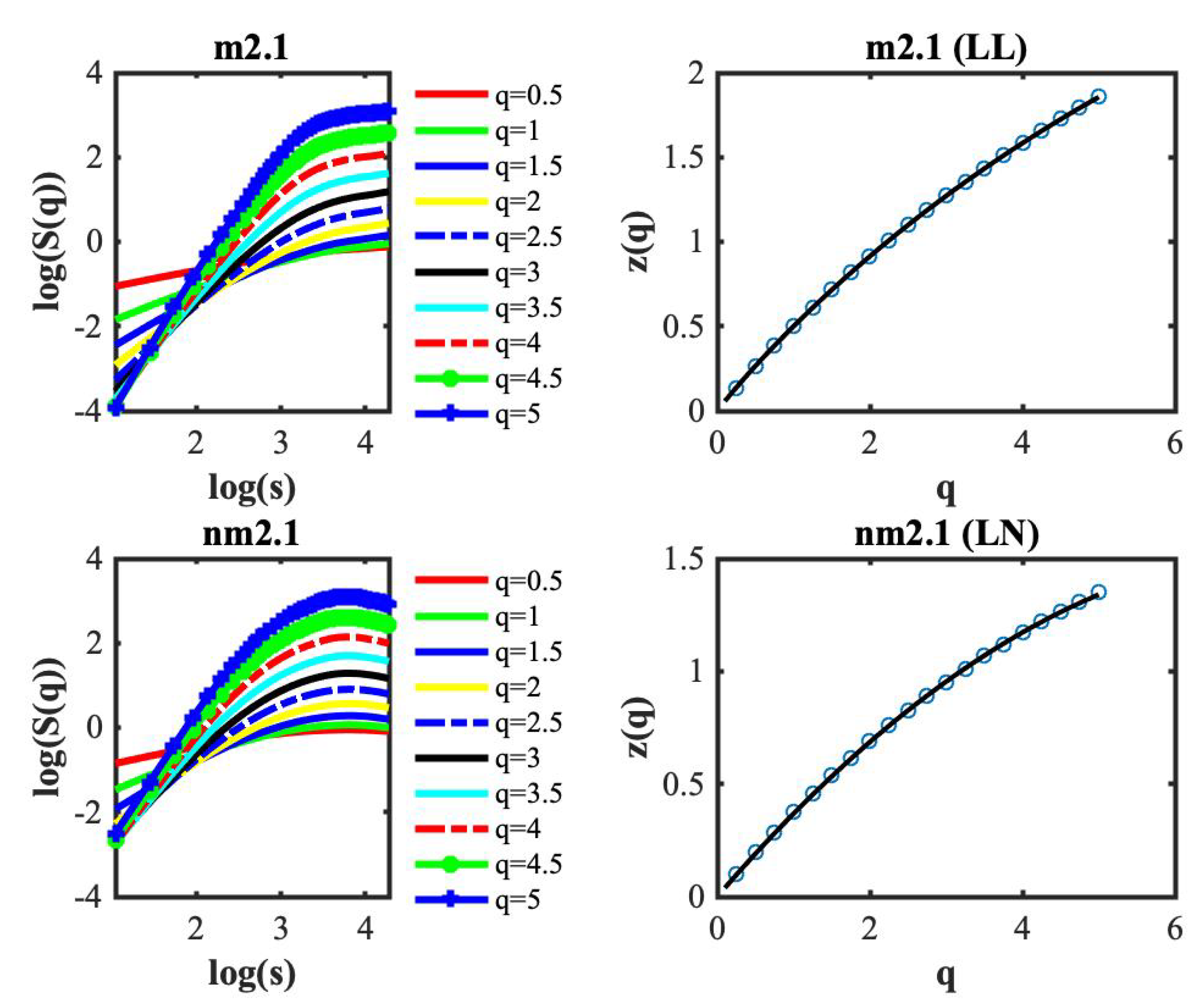
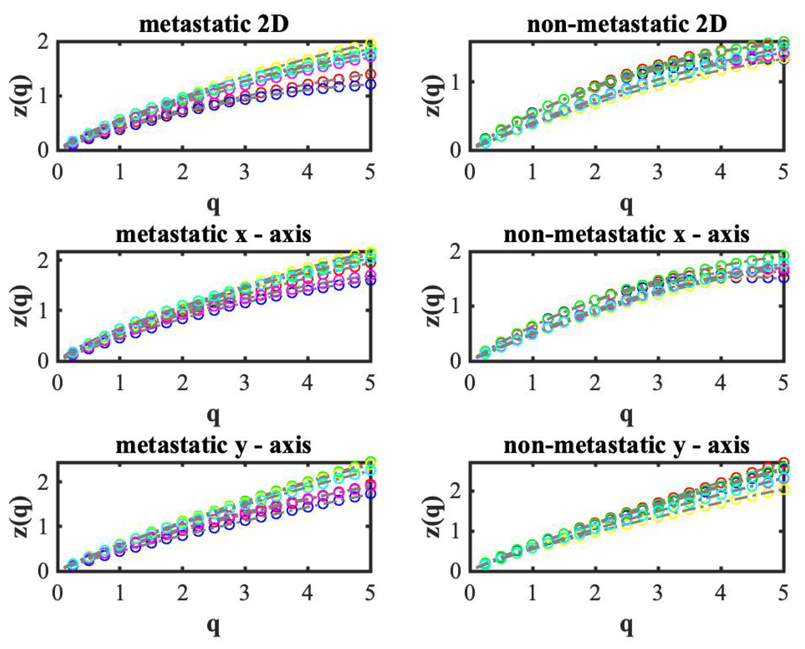
| 2D GMM | Two-dimensional generalized moments method |
Appendix A. Multifractal Detrended Fluctuation Analysis in Two Dimensions (2D-MFDFA)
Appendix B. Generalized Moments Method in Two Dimensions (2D-GMM)
Appendix C. Analysis of Raw Data

| 2D-GMM | GMM (x-Axis) | GMM (y-Axis) | |||||||
|---|---|---|---|---|---|---|---|---|---|
| Sample | H | C | H | C | H | C | |||
| m1.1 | 1 | 1 | 1 | ||||||
| m2.1 | 1 | ||||||||
| m2.2 | 1 | ||||||||
| m3.1 | 1 | ||||||||
| m3.2 | 1 | 1 | 1 | ||||||
| m3.3 | 1 | 1 | 1 | ||||||
| m3.4 | |||||||||
| m3.5 | 1 | 1 | 1 | ||||||
| m3.6 | 1 | 1 | 1 | ||||||
| nm1.1 | 2 | 2 | 1 | ||||||
| nm1.2 | 2 | 2 | 1 | ||||||
| nm1.3 | 1 | ||||||||
| nm2.1 | 2 | 2 | 1 | ||||||
| nm2.2 | 2 | 2 | 1 | ||||||
| nm2.3 | 2 | 2 | 1 | ||||||
References
- Fares, J.; Fares, M.Y.; Khachfe, H.H.; Salhab, H.A.; Fares, Y. Molecular principles of metastasis: A hallmark of cancer revisited. Signal Transduct. Target. Ther. 2020, 5, 28. [Google Scholar] [CrossRef] [PubMed]
- Esposito, M.; Ganesan, S.; Kang, Y. Emerging strategies for treating metastasis. Nat. Cancer 2021, 2, 258–270. [Google Scholar] [CrossRef] [PubMed]
- Chatter, C.L.; Weinberg, R.A. A perspective on cancer cell metastasis. Science 2011, 331, 1559–1564. [Google Scholar] [CrossRef]
- Lambert, A.W.; Pattabiraman, D.R.; Weinberg, R.A. Emerging Biological Principles of Metastasis. Cell 2017, 168, 670–691. [Google Scholar] [CrossRef] [Green Version]
- Fouad, Y.A.; Aanei, C. Revisiting the hallmarks of cancer. Am. J. Cancer Res. 2017, 7, 1016–1036. [Google Scholar]
- Vu, T.; Datta, P.K. Regulation of EMT in Colorectal Cancer: A Culprit in Metastasis. Cancers 2017, 9, 171. [Google Scholar] [CrossRef] [Green Version]
- Agus, D.B.; Alexander, J.F.; Arap, W.; Ashili, S.; Aslan, J.E.; Austin, R.H.; Backman, V.; Bethel, K.J.; Bonneau, R.; Chen, W.-C.; et al. A physical sciences network characterization of non-tumorigenic and metastatic cells. Sci. Rep. 2013, 3, 1449. [Google Scholar] [CrossRef]
- Rother, J.; Nöding, H.; Mey, I.; Janshoff, A. Atomic force microscopy-based microrheology reveals significant differences in the viscoelastic response between malign and benign cell lines. Open Biol. 2014, 4, 140046. [Google Scholar] [CrossRef]
- Baghban, R.; Roshangar, L.; Jahanban-Esfahlan, R.; Seidi, K.; Ebrahimi-Kalan, A.; Jaymand, M.; Kolahian, S.; Javaheri, T.; Zare, P. Tumor microenvironment complexity and therapeutic implications at a glance. Cell Commun. Signal. 2020, 18, 59. [Google Scholar] [CrossRef] [Green Version]
- Runel, G.; Lopez-Ramirez, N.; Chlasta, J.; Masse, I. Biomechanical Properties of Cancer Cells. Cells 2021, 10, 887. [Google Scholar] [CrossRef]
- Wang, R.; Dang, M.; Harada, K.; Han, G.; Wang, F.; Pizzi, M.P.; Zhao, M.; Tatlonghari, G.; Zhang, S.; Hao, D.; et al. Single-cell dissection of intratumoral heterogeneity and lineage diversity in metastatic gastric adenocarcinoma. Nat. Med. 2021, 27, 141–151. [Google Scholar] [CrossRef]
- Barabasi, A.L.; Vicsek, T. Multifractality of self-affine fractals. Phys. Rev. A 1991, 44, 2730–2733. [Google Scholar] [CrossRef]
- Meakin, P. The growth of rough surfaces and interfaces. Phys. Rep. 1993, 235, 189–289. [Google Scholar] [CrossRef]
- Kwapieńa, J.; Drożdż, S. Physical approach to complex systems. Phys. Rep. 2012, 515, 115–226. [Google Scholar] [CrossRef]
- Sedivy, R.; Mader, R.M. Fractals, Chaos, and Cancer: Do They Coincide? Cancer Investig. 1997, 15, 601–607. [Google Scholar] [CrossRef]
- Baish, J.W.; Jain, R.K. Fractals and Cancer. Cancer Res. 2000, 60, 3683–3688. [Google Scholar]
- Kosmou, A.; Sachpekidis, C.; Pan, L.; Matsopoulos, G.K.; Hassel, J.C.; Dimitrakopoulou-Strauss, A.; Provata, A. Fractal and Multifractal Analysis of PET-CT Images for Therapy Assessment of Metastatic Melanoma Patients under PD-1 Inhibitors: A Feasibility Study. Cancers 2021, 13, 5170. [Google Scholar] [CrossRef]
- Mezheyeuski, A.; Hrynchyk, I.; Karlberg, M.; Portyanko, A.; Egevad, L.; Ragnhammar, P.; Edler, D.; Glimelius, B.; Östman, A. Image analysis-derived metrics of histomorphological complexity predicts prognosis and treatment response in stage II–III colon cancer. Sci. Rep. 2016, 6, 36149. [Google Scholar] [CrossRef]
- Zhong, H.; Wang, J.; Hu, W.; Shen, L.; Wan, J.; Zhou, Z.; Zhang, Z. Fractal Dimension Analysis of Edge-Detected Rectal Cancer CTs for Outcome Prediction. Biomed. Med. Phys. 2015, 42, 3213. [Google Scholar] [CrossRef]
- da Silva, L.G.; da Silva Monteiro, W.R.S.; de Aguiar Moreira, T.M.; Rabelo, M.A.E.; de Assis, E.A.C.P.; de Souza, G.T. Fractal dimension analysis as an easy computational approach to improve breast cancer histopathological diagnosis. Appl. Microsc. 2021, 51, 6. [Google Scholar] [CrossRef]
- Chan, A.; Tuszynski, J.A. Automatic prediction of tumour malignancy in breast cancer with fractal dimension. R. Soc. Open Sci. 2016, 3, 160558. [Google Scholar] [CrossRef] [PubMed] [Green Version]
- Ohri, S.; Dey, P.; Nijhawan, R. Fractal dimension in aspiration cytology smears of breast and cervical lesions. Anal. Quant. Cytol. Histol. 2004, 26, 109–112. [Google Scholar]
- Mandelbrot, B.B. The Fractal Geometry of Nature; W. H. Freeman: New York, NY, USA, 1983. [Google Scholar]
- Lennon, F.E.; Cianci, G.C.; Cipriani, N.A.; Hensing, T.A.; Zhang, H.J.; Chen, C.-T.; Murgu, S.D.; Vokes, E.E.; Vannier, M.W.; Salgia, R. Lung cancer—A fractal viewpoint. Nat. Rev. Clin. Oncol. 2015, 12, 664–675. [Google Scholar] [CrossRef] [PubMed] [Green Version]
- Kestener, P.; Lina, J.M.; Saint-Jean, P.; Arneodo, A. Wavelet-based multifractal formalism to assist in diagnosis in digitized mammograms. Image Anal. Stereol. 2001, 20, 169–174. [Google Scholar] [CrossRef] [Green Version]
- Ramírez-Cobo, P.; Vidakovic, B. A 2D wavelet-based multiscale approach with applications to the analysis of digital mammograms. Comput. Stat. Data Anal. 2013, 58, 71–81. [Google Scholar] [CrossRef]
- Guz, N.V.; Dokukin, M.E.; Woodworth, C.D.; Cardina, A.; Sokolov, I. Towards early detection of cervical cancer: Fractal dimension of AFM images of human cervical epithelial cells at different stages of progression to cancer. Nanomedicine 2015, 11, 1667–1675. [Google Scholar] [CrossRef] [PubMed] [Green Version]
- Gneiting, T.; Sevcikova, H.; Perci, D.B. Estimators of Fractal Dimension: Assessing the Roughness of Time Series and Spatial Data. Stat. Sci. 2012, 27, 247–277. [Google Scholar] [CrossRef]
- Lopes, R.; Betrouni, N. Fractal and multifractal analysis: A review. Med. Image Anal. 2009, 13, 634–649. [Google Scholar] [CrossRef]
- Halley, J.M.; Hartley, S.; Kallimanis, A.S.; Kunin, W.E.; Lennon, J.J.; Sgardelis, S.P. Uses and abuses of fractal methodology in ecology. Eco. Lett. 2004, 7, 254–271. [Google Scholar] [CrossRef]
- Hall, P.; Roy, R. On the relationship between fractal dimension and fractal index for stationary stochastic processes. Ann. Appl. Probab. 1994, 4, 241–253. [Google Scholar] [CrossRef]
- Xue, Y.; Xiao, Y. Fractal and smoothness properties of space–time Gaussian models. Front. Math. China 2011, 6, 1217–1248. [Google Scholar] [CrossRef]
- Cheng, Q. Multifractality and spatial statistics. Comput. Geosci. 1999, 25, 949–961. [Google Scholar] [CrossRef]
- Bizzarri, M.; Giuliani, A.; Cucina, A.; D’Anselmi, F.; Soto, A.M.; Sonnenschein, C. Fractal analysis in a systems biology approach to cancer. Semin. Cancer Biol. 2011, 21, 175–182. [Google Scholar] [CrossRef] [Green Version]
- Meacham, C.E.; Morrison, S.J. Tumor heterogeneity and cancer cell plasticity. Nature 2013, 501, 328–337. [Google Scholar] [CrossRef] [Green Version]
- Barabasi, A.-L.; Stanley, H.E. Fractal Concepts in Surface Growth; Cambridge University Press: Cambridge, MA, USA, 1995. [Google Scholar] [CrossRef]
- Das, N.; Alexandrov, S.; Gilligan, K.E.; Dwyer, R.M.; Saager, R.B.; Ghosh, N.; Leahy, M. Characterization of nanosensitive multifractality in submicron scale tissue morphology and its alteration in tumor progression. J. Biomed. Opt. 2021, 26, 16003. [Google Scholar] [CrossRef]
- Xu, J.; Galvanetto, N.; Nie, J.; Yang, Y.; Torre, V. Rac1 Promotes Cell Motility by Controlling Cell Mechanics in Human Glioblastoma. Cancers 2020, 12, 1667. [Google Scholar] [CrossRef]
- Hohmann, T.; Hohmann, U.; Dahlmann, M.; Kobelt, D.; Stein, U.; Dehghani, F. MACC1-Induced Collective Migration Is Promoted by Proliferation Rather Than Single Cell Biomechanics. Cancers 2022, 14, 2857. [Google Scholar] [CrossRef]
- Bemmerlein, L.; Deniz, I.A.; Karbanová, J.; Jacobi, A.; Drukewitz, S.; Link, T.; Göbel, A.; Sevenich, L.; Taubenberger, A.V.; Wimberger, P.; et al. Decoding Single Cell Morphology in Osteotropic Breast Cancer Cells for Dissecting Their Migratory, Molecular and Biophysical Heterogeneity. Cancers 2022, 14, 603. [Google Scholar] [CrossRef]
- Tsitlakidis, A.; Tsingotjidou, A.S.; Kritis, A.; Cheva, A.; Selviaridis, P.; Aifantis, E.C.; Foroglou, N. Atomic Force Microscope Nanoindentation Analysis of Diffuse Astrocytic Tumor Elasticity: Relation with Tumor Histopathology. Cancers 2021, 13, 4539. [Google Scholar] [CrossRef]
- Adhikari, P.; Hasan, M.; Sridhar, V.; Roy, D.; Pradhan, P. Studying nanoscale structural alterations in cancer cells to evaluate ovarian cancer drug treatment, using transmission electron microscopy imaging. Phys. Biol. 2020, 17, 36005. [Google Scholar] [CrossRef]
- Zemła, J.; Danilkiewicz, J.; Orzechowska, B.; Pabijan, J.; Seweryn, S.; Lekka, M. Atomic force microscopy as a tool for assessing the cellular elasticity and adhesiveness to identify cancer cells and tissues. Semin. Cell Dev. Biol. 2018, 73, 115–124. [Google Scholar] [CrossRef] [PubMed]
- Deng, X.; Xiong, F.; Li, X.; Xiang, B.; Li, Z.; Wu, X.; Guo, C.; Li, X.; Li, Y.; Li, G.; et al. Application of atomic force microscopy in cancer research. J. Nanobiotechnol. 2018, 16, 102. [Google Scholar] [CrossRef] [PubMed] [Green Version]
- Tiribilli, B.; Bani, D.; Quercioli, F.; Ghirelli, A.; Vassalli, A.M. Atomic force microscopy of histological sections using a chemical etching method. Ultramicroscopy 2005, 102, 227–232. [Google Scholar] [CrossRef] [PubMed]
- Azzalini, E.; Abdurakhmanova, N.; Parisse, P.; Bartoletti, M.; Canzonieri, V.; Stanta, G.; Casalis, L.; Bonin, S. Cell-stiffness and morphological architectural patterns in clinical samples of high grade serous ovarian cancers. Nanomed. Nanotechnol. Biol. Med. 2021, 37, 102452. [Google Scholar] [CrossRef]
- Hosokawa, M.; Kenmotsu, H.; Koh, Y.; Yoshino, T.; Yoshikawa, T.; Naito, T.; Takahashi, T.; Murakami, H.; Nakamura, Y.; Tsuya, A.; et al. Size-Based Isolation of Circulating Tumor Cells in Lung Cancer Patients Using a Microcavity Array System. PLoS ONE 2013, 8, e67466. [Google Scholar] [CrossRef] [Green Version]
- Kantelhardt, J.W.; Zschiegner, S.A.; Koscielny-Bunde, E.; Havlin, S.; Bunde, A.; Stanley, H.E. Multifractal detrended fluctuation analysis of nonstationary time series. Physica A 2002, 316, 87–114. [Google Scholar] [CrossRef] [Green Version]
- Gu, G.-F.; Zhou, W.-X. Detrended fluctuation analysis for fractals and multifractals in higher dimensions. Phys. Rev. E 2006, 74, 061104. [Google Scholar] [CrossRef] [Green Version]
- Bakalis, E.; Höfinger, S.; Venturini, A.; Zerbetto, F. Crossover of two power laws in the anomalous diffusion of a two lipid membrane. J. Chem. Phys. 2015, 142, 215102. [Google Scholar] [CrossRef]
- Sändig, N.; Bakalis, E.; Zerbetto, F. Stochastic analysis of movements on surfaces: The case of C60 on Au(1 1 1). Chem. Phys. Lett. 2015, 633, 163–168. [Google Scholar] [CrossRef]
- Parent, L.R.; Bakalis, E.; Proetto, M.; Li, Y.; Park, C.; Zerbetto, F.; Gianneschi, N.C. Tackling the Challenges of Dynamic Experiments Using Liquid-Cell Transmission Electron Microscopy. Acc. Chem. Res. 2018, 51, 3–11. [Google Scholar] [CrossRef]
- Bakalis, E.; Parent, L.R.; Vratsanos, M.; Park, C.; Gianneschi, N.C.; Zerbetto, F. Complex Nanoparticle Diffusional Motion in Liquid-Cell Transmission Electron Microscopy. J. Phys. Chem. C 2020, 127, 14881–14890. [Google Scholar] [CrossRef]
- Bakalis, E.; Gavriil, V.; Cefalas, Z.-C.; Kollia, Z.; Zerbetto, F.; Sarantopoulou, E. Viscoelasticity and Noise Properties Reveal the Formation of Biomemory in Cells. J. Phys. Chem. B. 2021, 125, 10883–10892. [Google Scholar] [CrossRef]
- Halsey, T.C.; Jensen, M.H.; Kadanoff, L.P.; Procaccia, I.; Shraiman, B.I. Fractal measures and their singularities: The characterization of strange sets. Phys. Rev. A 1986, 33, 1141. [Google Scholar] [CrossRef]
- Carbone, A. Algorithm to estimate the Hurst exponent of high-dimensional fractals. Phys. Rev. E 2007, 76, 056703. [Google Scholar] [CrossRef] [Green Version]
- Di Matteo, T. Multi-scaling in finance. Quant. Financ. 2007, 7, 21–36. [Google Scholar] [CrossRef]
- Ponson, L.; Bonamy, D.; Bouchaud, E. Two-dimensional scaling properties of experimental fracture surfaces. Phys. Rev. Lett. 2006, 96, 035506. [Google Scholar] [CrossRef] [Green Version]
- Parent, L.R.; Bakalis, E.; Ramirez-Hernandez, A.; Kammeyer, J.K.; Park, C.; de Pablo, J.; Zerbetto, F.; Patterson, J.P.; Gianneschi, N.C. Directly Observing Micelle Fusion and Growth in Solution by Liquid- Cell Transmission Electron Microscopy. J. Am. Chem. Soc. 2017, 139, 17140–17151. [Google Scholar] [CrossRef]
- Andersen, K.; Castiglione, P.; Mazzino, A.; Vulpiani, A. Simple stochastic models showing strong anomalous diffusion. Eur. Phys. J. B 2000, 18, 447–452. [Google Scholar] [CrossRef] [Green Version]
- Schertzer, D.; Lovejoy, S. Physical modeling and Analysis of Rain and Clouds by Anisotropic Scaling of Multiplicative Processes. J. Geophys. Res. 1987, 92, 9693–9714. [Google Scholar] [CrossRef]
- Hurst, H.E. Long-term storage capacity of reservoirs. Trans. Am. Soc. Civ. Eng. 1951, 116, 770–799. [Google Scholar] [CrossRef]
- Kolmogorov, A.N. A refinement of previous hypotheses concerning the local structure of turbulence in a viscous incompressible fluid at high Reynolds number. J. Fluid Mech. 1962, 13, 82–85. [Google Scholar] [CrossRef] [Green Version]


Publisher’s Note: MDPI stays neutral with regard to jurisdictional claims in published maps and institutional affiliations. |
© 2022 by the authors. Licensee MDPI, Basel, Switzerland. This article is an open access article distributed under the terms and conditions of the Creative Commons Attribution (CC BY) license (https://creativecommons.org/licenses/by/4.0/).
Share and Cite
Bakalis, E.; Ferraro, A.; Gavriil, V.; Pepe, F.; Kollia, Z.; Cefalas, A.-C.; Malapelle, U.; Sarantopoulou, E.; Troncone, G.; Zerbetto, F. Universal Markers Unveil Metastatic Cancerous Cross-Sections at Nanoscale. Cancers 2022, 14, 3728. https://doi.org/10.3390/cancers14153728
Bakalis E, Ferraro A, Gavriil V, Pepe F, Kollia Z, Cefalas A-C, Malapelle U, Sarantopoulou E, Troncone G, Zerbetto F. Universal Markers Unveil Metastatic Cancerous Cross-Sections at Nanoscale. Cancers. 2022; 14(15):3728. https://doi.org/10.3390/cancers14153728
Chicago/Turabian StyleBakalis, Evangelos, Angelo Ferraro, Vassilios Gavriil, Francesco Pepe, Zoe Kollia, Alkiviadis-Constantinos Cefalas, Umberto Malapelle, Evangelia Sarantopoulou, Giancarlo Troncone, and Francesco Zerbetto. 2022. "Universal Markers Unveil Metastatic Cancerous Cross-Sections at Nanoscale" Cancers 14, no. 15: 3728. https://doi.org/10.3390/cancers14153728
APA StyleBakalis, E., Ferraro, A., Gavriil, V., Pepe, F., Kollia, Z., Cefalas, A.-C., Malapelle, U., Sarantopoulou, E., Troncone, G., & Zerbetto, F. (2022). Universal Markers Unveil Metastatic Cancerous Cross-Sections at Nanoscale. Cancers, 14(15), 3728. https://doi.org/10.3390/cancers14153728