
Automatic Brain Tissue and Lesion Segmentation and Multi-Parametric Mapping of Contrast-Enhancing Gliomas without the Injection of Contrast Agents: A Preliminary Study

 ,
,
Abstract
:Simple Summary
Abstract
1. Introduction
2. Materials and Methods
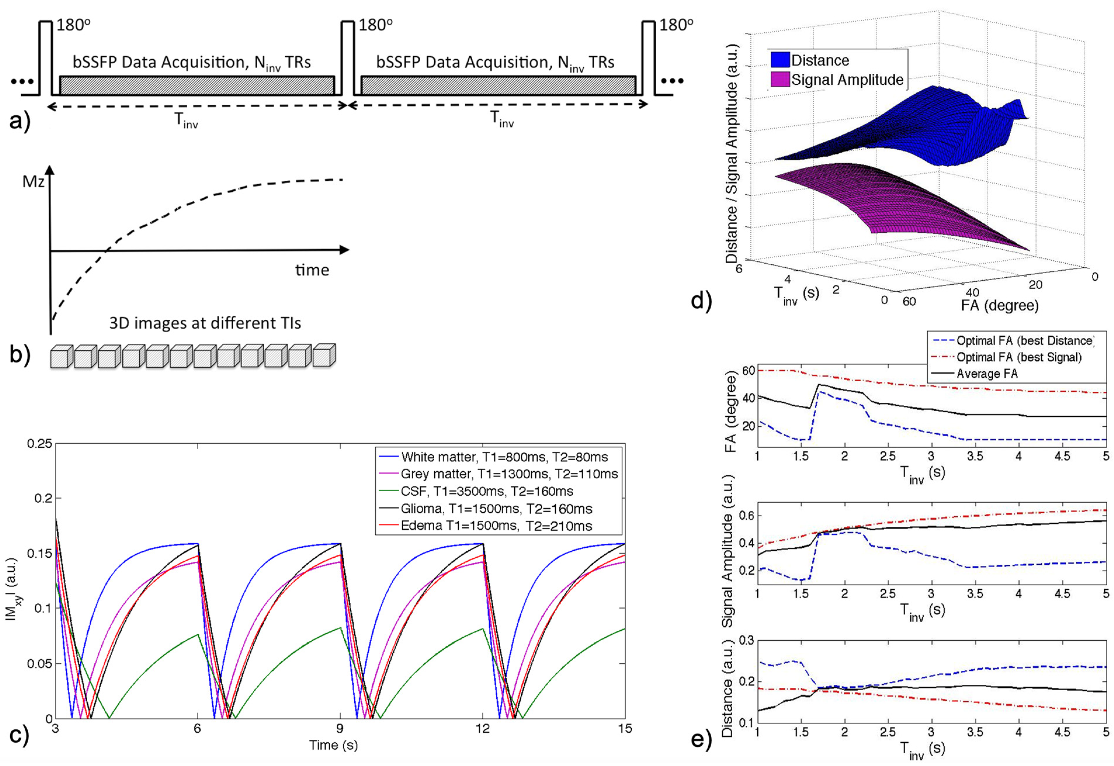
2.1. IIR-bSSFP Acquisition
2.2. Optimization of Scan Parameters
2.3. Acceleration and Image Reconstruction
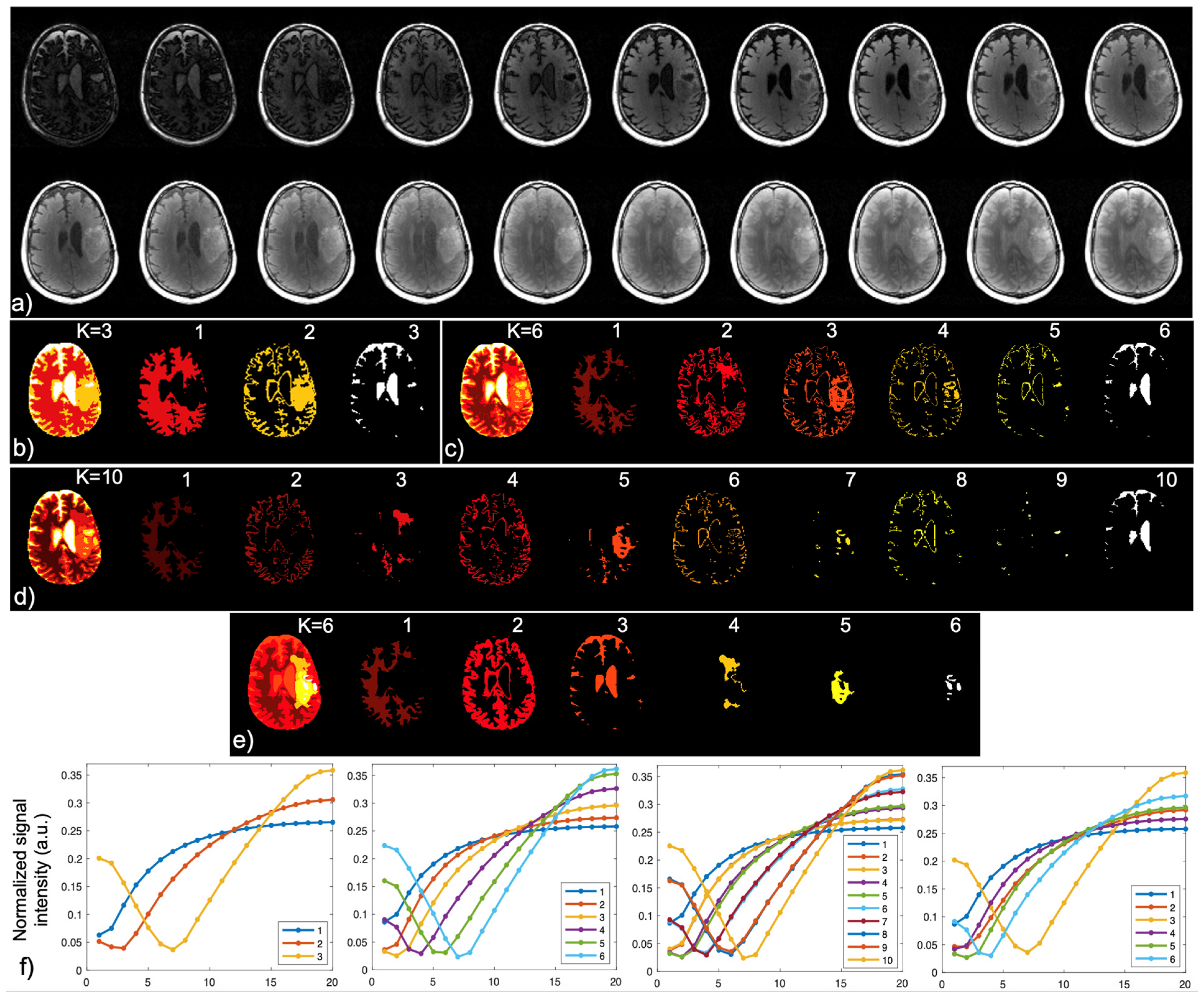
2.4. Brain Tissue and Lesion Segmentation
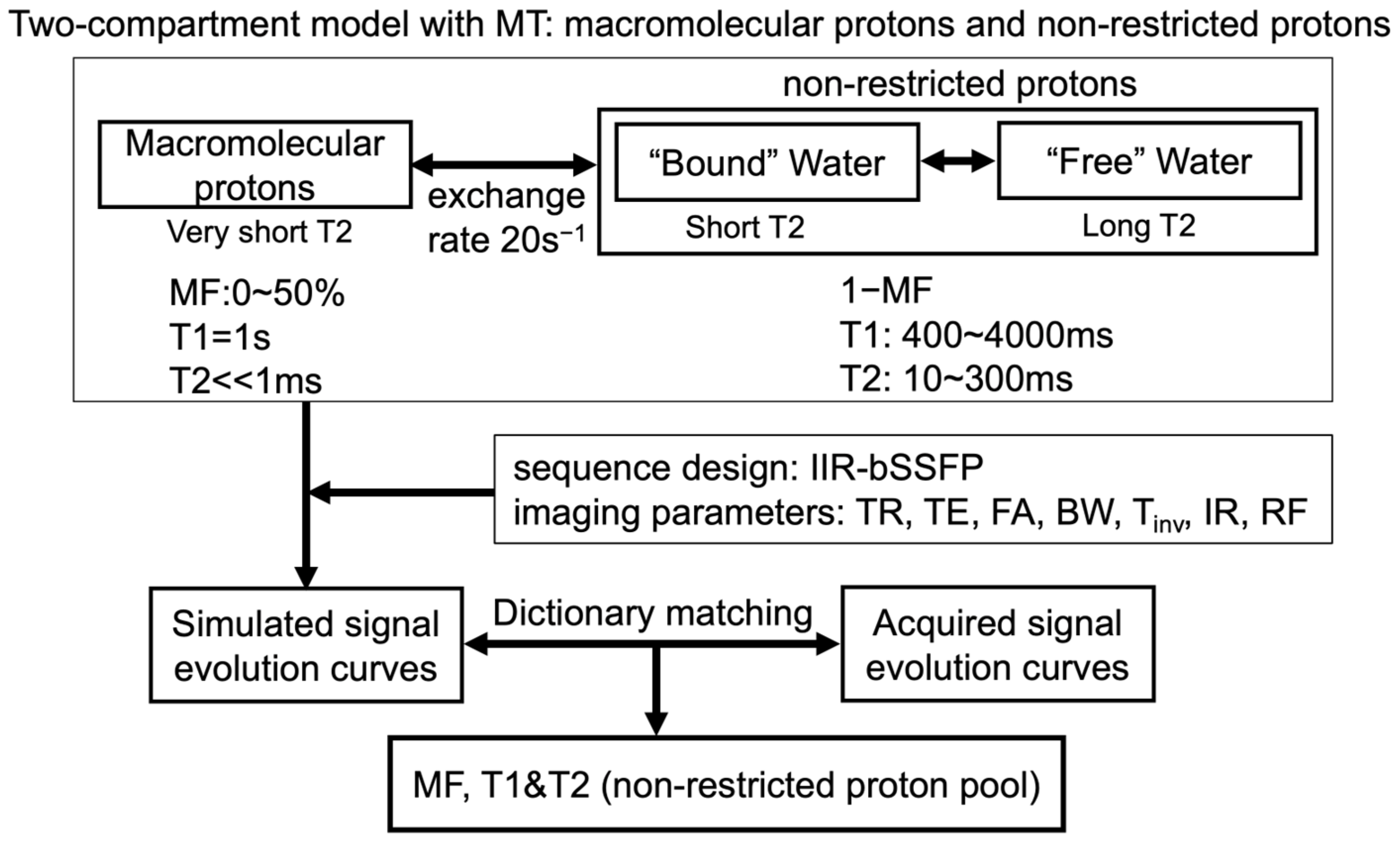
2.5. Two-Compartment Modeling and Multi-Parametric Mapping
2.6. Patient Scans
2.7. Data Analysis
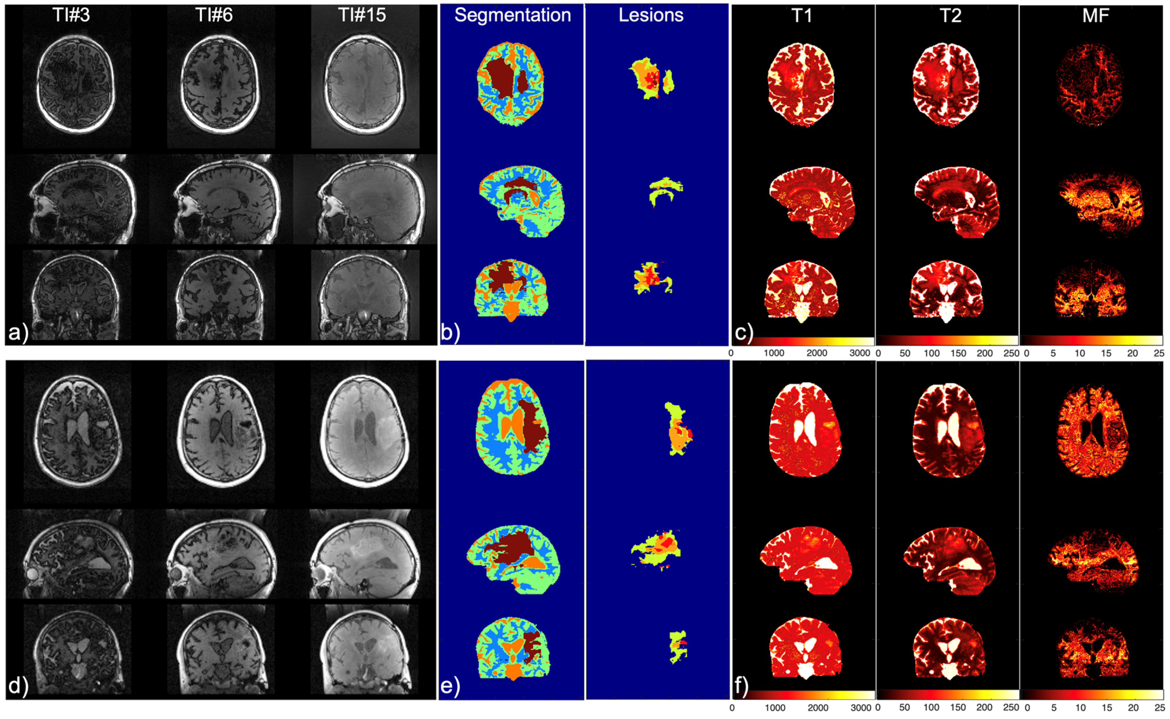
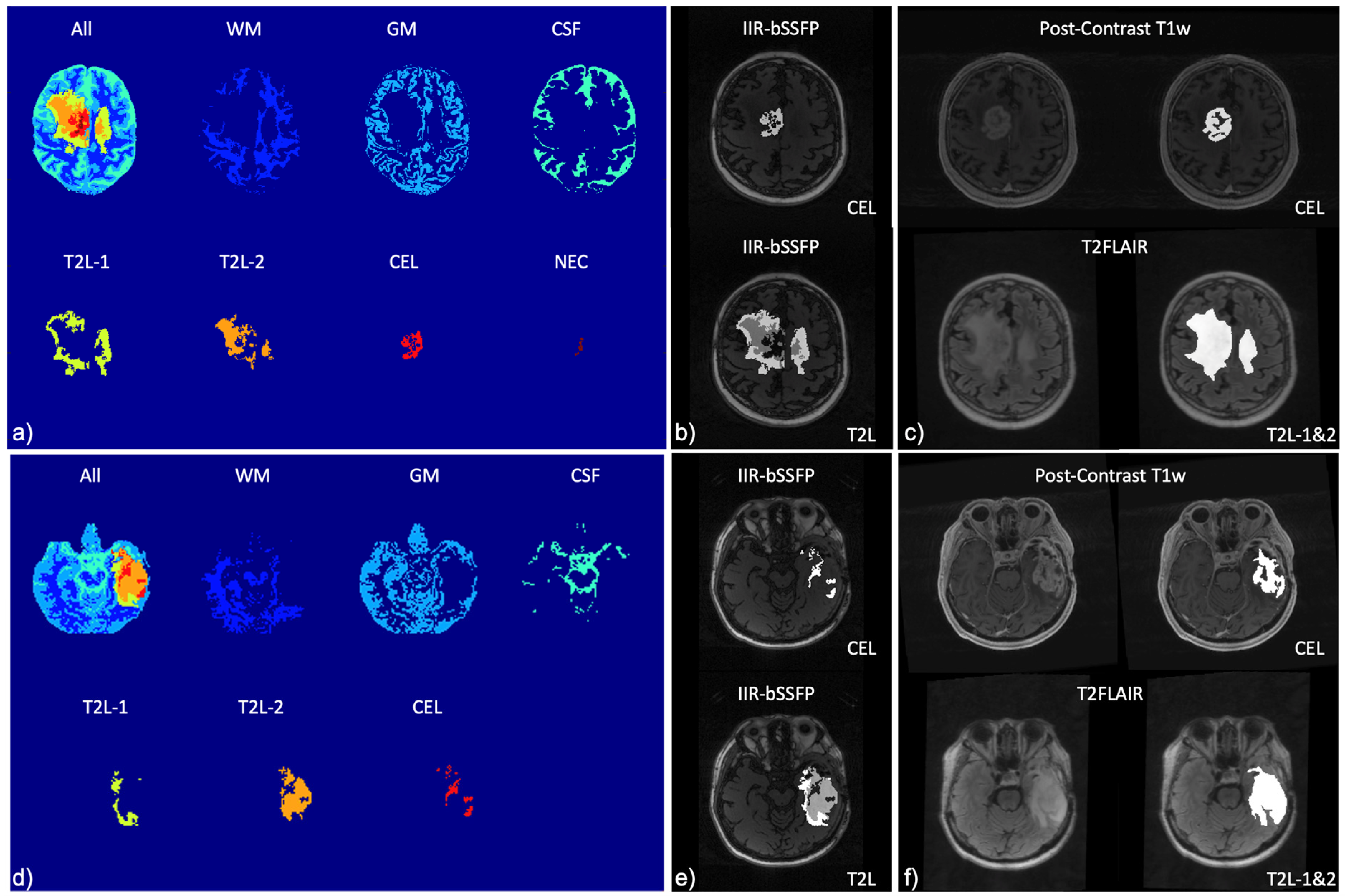
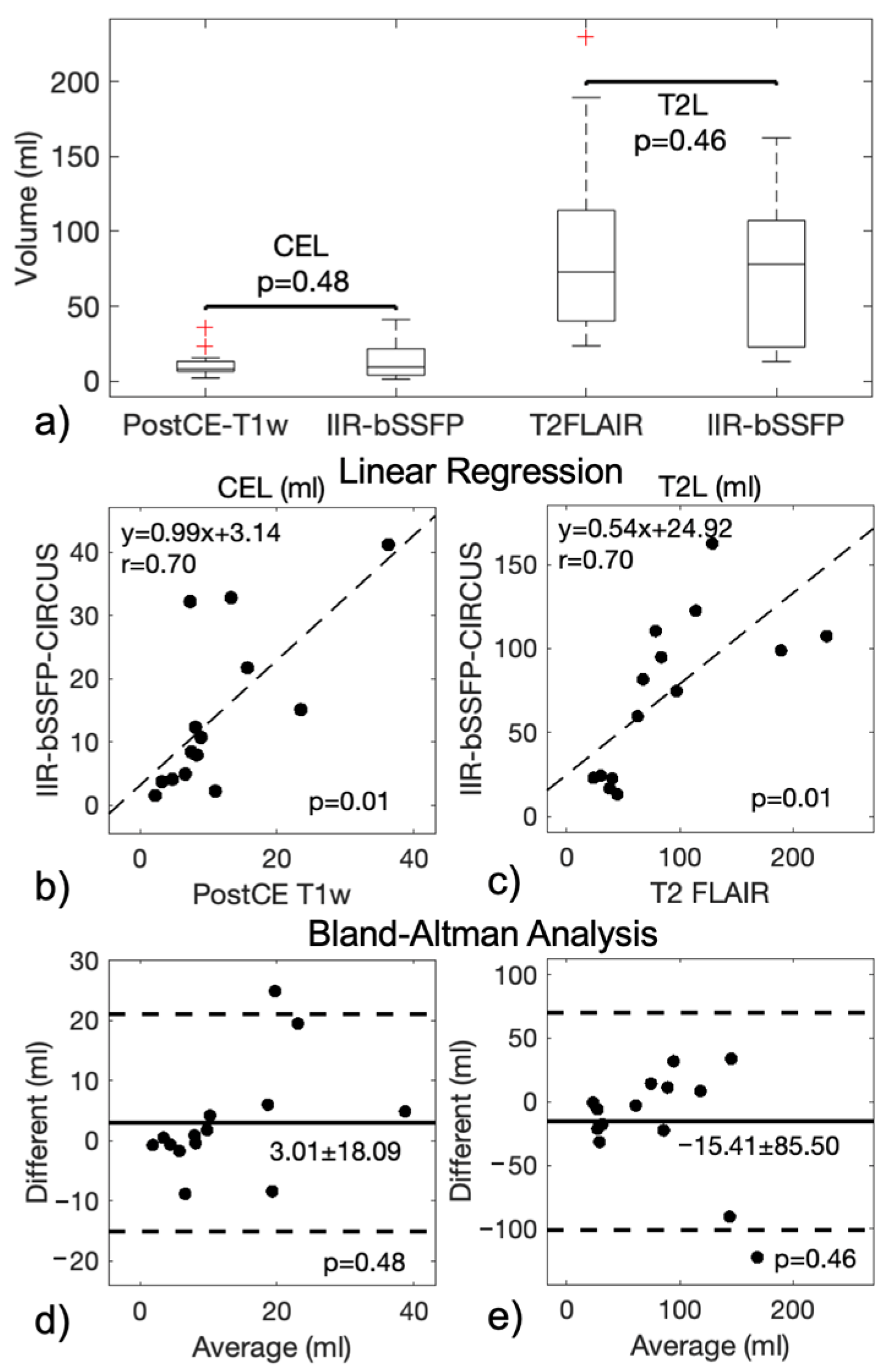
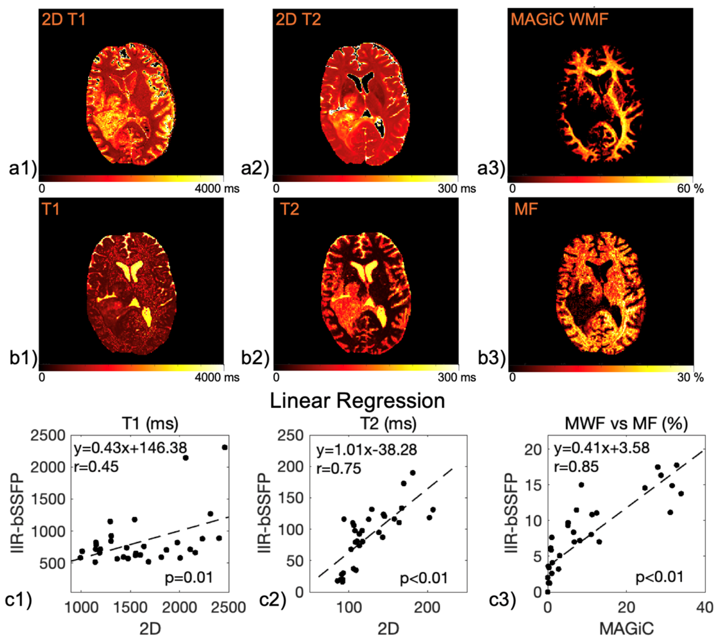
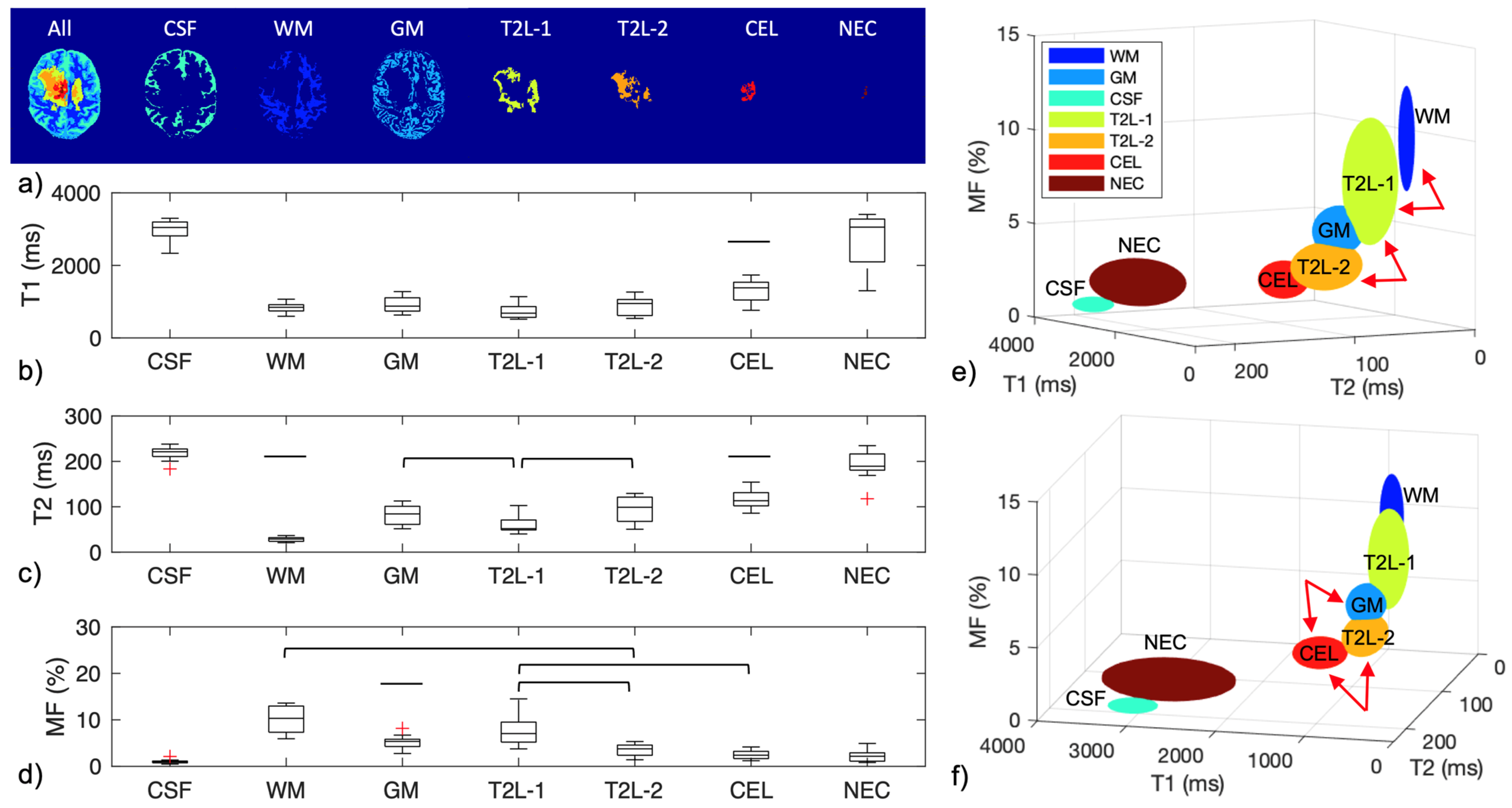
3. Results
4. Discussion
5. Conclusions
Author Contributions
Funding
Institutional Review Board Statement
Informed Consent Statement
Data Availability Statement
Acknowledgments
Conflicts of Interest
References
- Louis, D.N.; Perry, A.; Reifenberger, G.; Von Deimling, A.; Figarella-Branger, D.; Cavenee, W.K.; Ohgaki, H.; Wiestler, O.D.; Kleihues, P.; Ellison, D.W. The 2016 World Health Organization Classification of Tumors of the Central Nervous System: A summary. Acta Neuropathol. 2016, 131, 803–820. [Google Scholar] [CrossRef] [PubMed]
- Ostrom, Q.T.; Gittleman, H.; Fulop, J.; Liu, M.; Blanda, R.; Kromer, C.; Wolinsky, Y.; Kruchko, C.; Barnholtz-Sloan, J.S. CBTRUS Statistical Report: Primary Brain and Central Nervous System Tumors Diagnosed in the United States in 2008-2012. Neuro Oncol. 2015, 17, iv1–iv62. [Google Scholar] [CrossRef] [PubMed]
- Louis, D.N.; Ohgaki, H.; Wiestler, O.D.; Cavenee, W.K.; Burger, P.C.; Jouvet, A.; Scheithauer, B.W.; Kleihues, P. The 2007 WHO Classification of Tumours of the Central Nervous System. Acta Neuropathol. 2007, 114, 97–109. [Google Scholar] [CrossRef] [PubMed]
- Giese, A.; Westphal, M. Treatment of malignant glioma: A problem beyond the margins of resection. J. Cancer Res. Clin. Oncol. 2001, 127, 217–225. [Google Scholar] [CrossRef] [PubMed]
- Ellingson, B.M.; Bendszus, M.; Boxerman, J.; Barboriak, D.; Erickson, B.J.; Smits, M.; Nelson, S.J.; Gerstner, E.; Alexander, B.; Goldmacher, G.; et al. Consensus recommendations for a standardized Brain Tumor Imaging Protocol in clinical trials. Neuro-Oncol. 2015, 17, 1188–1198. [Google Scholar] [CrossRef] [PubMed]
- Leu, K.; Pope, W.B.; Cloughesy, T.F.; Lai, A.; Nghiemphu, P.L.; Chen, W.; Liau, L.M.; Ellingson, B.M. Imaging biomarkers for antiangiogenic therapy in malignant gliomas. CNS Oncol. 2013, 2, 33–47. [Google Scholar] [CrossRef] [PubMed]
- Huse, J.T.; Wallace, M.; Aldape, K.D.; Berger, M.S.; Bettegowda, C.; Brat, D.J.; Cahill, D.P.; Cloughesy, T.; Haas-Kogan, D.A.; Marra, M.; et al. Where are we now? And where are we going? A report from the Accelerate Brain Cancer Cure (ABC2) Low-grade Glioma Research Workshop. Neuro-Oncol. 2014, 16, 173–178. [Google Scholar] [CrossRef] [PubMed]
- Norden, A.D.; Drappatz, J.; Muzikansky, A.; David, K.; Gerard, M.; McNamara, M.B.; Phan, P.; Ross, A.; Kesari, S.; Wen, P.Y. An exploratory survival analysis of anti-angiogenic therapy for recurrent malignant glioma. J. Neurooncol. 2009, 92, 149–155. [Google Scholar] [CrossRef] [PubMed]
- Wen, P.Y.; Van Den Bent, M.; Youssef, G.; Cloughesy, T.F.; Ellingson, B.M.; Weller, M.; Galanis, E.; Barboriak, D.P.; De Groot, J.; Gilbert, M.R.; et al. RANO 2.0: Update to the Response Assessment in Neuro-Oncology Criteria for High- and Low-Grade Gliomas in Adults. J. Clin. Oncol. 2023, 41, 5187–5199. [Google Scholar] [CrossRef] [PubMed]
- Menze, B.H.; Jakab, A.; Bauer, S.; Kalpathy-Cramer, J.; Farahani, K.; Kirby, J.; Burren, Y.; Porz, N.; Slotboom, J.; Wiest, R.; et al. The Multimodal Brain Tumor Image Segmentation Benchmark (BRATS). IEEE Trans. Med. Imaging 2015, 34, 1993–2024. [Google Scholar] [CrossRef] [PubMed]
- Meier, R.; Bauer, S.; Slotboom, J.; Wiest, R.; Reyes, M. Appearance-and Context-sensitive Features for Brain Tumor Segmentation. In Proceedings of the MICCAI BRATS Challenge, Boston, MA, USA, 14 September 2014. [Google Scholar] [CrossRef]
- Porz, N.; Bauer, S.; Pica, A.; Schucht, P.; Beck, J.; Verma, R.K.; Slotboom, J.; Reyes, M.; Wiest, R. Multi-Modal Glioblastoma Segmentation: Man versus Machine. PLoS ONE 2014, 9, e96873. [Google Scholar] [CrossRef] [PubMed]
- Steed, T.C.; Treiber, J.M.; Patel, K.S.; Taich, Z.; White, N.S.; Treiber, M.L.; Farid, N.; Carter, B.S.; Dale, A.M.; Chen, C.C. Iterative Probabilistic Voxel Labeling: Automated Segmentation for Analysis of the Cancer Imaging Archive Glioblastoma Images. AJNR Am. J. Neuroradiol. 2015, 36, 678–685. [Google Scholar] [CrossRef] [PubMed]
- Weizman, L.; Sira, L.B.; Joskowicz, L.; Rubin, D.L.; Yeom, K.W.; Constantini, S.; Shofty, B.; Bashat, D.B. Semiautomatic segmentation and follow-up of multicomponent low-grade tumors in longitudinal brain MRI studies: Segmentation and follow-up of low-grade tumors. Med. Phys. 2014, 41, 052303. [Google Scholar] [CrossRef]
- Liberman, G.; Louzoun, Y.; Aizenstein, O.; Blumenthal, D.T.; Bokstein, F.; Palmon, M.; Corn, B.W.; Ben Bashat, D. Automatic multi-modal MR tissue classification for the assessment of response to bevacizumab in patients with glioblastoma. Eur. J. Radiol. 2013, 82, e87–e94. [Google Scholar] [CrossRef]
- Meier, R.; Knecht, U.; Loosli, T.; Bauer, S.; Slotboom, J.; Wiest, R.; Reyes, M. Clinical Evaluation of a Fully-automatic Segmentation Method for Longitudinal Brain Tumor Volumetry. Sci. Rep. 2016, 6, 23376. [Google Scholar] [CrossRef] [PubMed]
- Vollmuth, P.; Foltyn, M.; Huang, R.Y.; Galldiks, N.; Petersen, J.; Isensee, F.; Van Den Bent, M.J.; Barkhof, F.; Park, J.E.; Park, Y.W.; et al. Artificial intelligence (AI)-based decision support improves reproducibility of tumor response assessment in neuro-oncology: An international multi-reader study. Neuro-Oncol. 2023, 25, 533–543. [Google Scholar] [CrossRef] [PubMed]
- Li, K.; Li, H.; Zhang, X.-Y.; Stokes, A.M.; Jiang, X.; Kang, H.; Quarles, C.C.; Zu, Z.; Gochberg, D.F.; Gore, J.C.; et al. Influence of water compartmentation and heterogeneous relaxation on quantitative magnetization transfer imaging in rodent brain tumors: Two-Pool qMT in Tumors. Magn. Reson. Med. 2016, 76, 635–644. [Google Scholar] [CrossRef] [PubMed]
- Mehrabian, H.; Myrehaug, S.; Soliman, H.; Sahgal, A.; Stanisz, G.J. Quantitative Magnetization Transfer in Monitoring Glioblastoma (GBM) Response to Therapy. Sci. Rep. 2018, 8, 2475. [Google Scholar] [CrossRef]
- Gu, W.; Fang, S.; Hou, X.; Ma, D.; Li, S. Exploring diagnostic performance of T2 mapping in diffuse glioma grading. Quant. Imaging Med. Surg. 2021, 11, 2943–2954. [Google Scholar] [CrossRef]
- Springer, E.; Cardoso, P.L.; Strasser, B.; Bogner, W.; Preusser, M.; Widhalm, G.; Nittka, M.; Koerzdoerfer, G.; Szomolanyi, P.; Hangel, G.; et al. MR Fingerprinting—A Radiogenomic Marker for Diffuse Gliomas. Cancers 2022, 14, 723. [Google Scholar] [CrossRef]
- Hattingen, E.; Jurcoane, A.; Daneshvar, K.; Pilatus, U.; Mittelbronn, M.; Steinbach, J.P.; Bahr, O. Quantitative T2 mapping of recurrent glioblastoma under bevacizumab improves monitoring for non-enhancing tumor progression and predicts overall survival. Neuro-Oncol. 2013, 15, 1395–1404. [Google Scholar] [CrossRef] [PubMed]
- Lescher, S.; Jurcoane, A.; Veit, A.; Bähr, O.; Deichmann, R.; Hattingen, E. Quantitative T1 and T2 mapping in recurrent glioblastomas under bevacizumab: Earlier detection of tumor progression compared to conventional MRI. Neuroradiology 2015, 57, 11–20. [Google Scholar] [CrossRef]
- Kern, M.; Auer, T.A.; Picht, T.; Misch, M.; Wiener, E. T2 mapping of molecular subtypes of WHO grade II/III gliomas. BMC Neurol. 2020, 20, 8. [Google Scholar] [CrossRef] [PubMed]
- Auer, T.A.; Kern, M.; Fehrenbach, U.; Tanyldizi, Y.; Misch, M.; Wiener, E. T2 mapping of the peritumoral infiltration zone of glioblastoma and anaplastic astrocytoma. Neuroradiol. J. 2021, 34, 392–400. [Google Scholar] [CrossRef] [PubMed]
- Oh, J.; Cha, S.; Aiken, A.H.; Han, E.T.; Crane, J.C.; Stainsby, J.A.; Wright, G.A.; Dillon, W.P.; Nelson, S.J. Quantitative apparent diffusion coefficients and T2 relaxation times in characterizing contrast enhancing brain tumors and regions of peritumoral edema. Magn. Reson. Imaging 2005, 21, 701–708. [Google Scholar] [CrossRef]
- Bieri, O.; Scheffler, K. Fundamentals of balanced steady state free precession MRI: Fundamentals of Balanced SSFP MRI. J. Magn. Reson. Imaging 2013, 38, 2–11. [Google Scholar] [CrossRef] [PubMed]
- Stanisz, G.J.; Odrobina, E.E.; Pun, J.; Escaravage, M.; Graham, S.J.; Bronskill, M.J.; Henkelman, R.M. T1, T2 relaxation and magnetization transfer in tissue at 3T. Magn. Reson. Med. 2005, 54, 507–512. [Google Scholar] [CrossRef]
- Deoni, S.C.L.; Rutt, B.K.; Arun, T.; Pierpaoli, C.; Jones, D.K. Gleaning multicomponent T1 and T2 information from steady-state imaging data. Magn. Reson. Med. 2008, 60, 1372–1387. [Google Scholar] [CrossRef] [PubMed]
- Wansapura, J.P.; Holland, S.K.; Dunn, R.S.; Ball, W.S. NMR relaxation times in the human brain at 3.0 tesla. J. Magn. Reson. Imaging 1999, 9, 531–538. [Google Scholar] [CrossRef]
- Bloch, F. Nuclear Induction. Phys. Rev. 1946, 70, 460–474. [Google Scholar] [CrossRef]
- Liu, J.; Saloner, D. Accelerated MRI with CIRcular Cartesian UnderSampling (CIRCUS): A variable density Cartesian sampling strategy for compressed sensing and parallel imaging. Quant. Imaging Med. Surg. 2014, 4, 57–67. [Google Scholar] [CrossRef] [PubMed]
- Liu, J.; Pedoia, V.; Heilmeier, U.; Ku, E.; Su, F.; Khanna, S.; Imboden, J.; Graf, J.; Link, T.; Li, X. High-temporospatial-resolution dynamic contrast-enhanced (DCE) wrist MRI with variable-density pseudo-random circular Cartesian undersampling (CIRCUS) acquisition: Evaluation of perfusion in rheumatoid arthritis patients: High Temporospatial Resolution DCE Wrist MRI. NMR Biomed. 2016, 29, 15–23. [Google Scholar] [CrossRef] [PubMed]
- Liu, J.; Feng, L.; Shen, H.-W.; Zhu, C.; Wang, Y.; Mukai, K.; Brooks, G.C.; Ordovas, K.; Saloner, D. Highly-accelerated self-gated free-breathing 3D cardiac cine MRI: Validation in assessment of left ventricular function. Magn. Reson. Mater. Phys. Biol. Med. 2017, 30, 337–346. [Google Scholar] [CrossRef] [PubMed]
- Liu, J.; Koskas, L.; Faraji, F.; Kao, E.; Wang, Y.; Haraldsson, H.; Kefayati, S.; Zhu, C.; Ahn, S.; Laub, G.; et al. Highly accelerated intracranial 4D flow MRI: Evaluation of healthy volunteers and patients with intracranial aneurysms. MAGMA 2018, 31, 295–307. [Google Scholar] [CrossRef] [PubMed]
- Liu, J.; Wang, Y.; Wen, Z.; Feng, L.; Lima, A.P.S.; Mahadevan, V.S.; Bolger, A.; Saloner, D.; Ordovas, K. Extending Cardiac Functional Assessment with Respiratory-Resolved 3D Cine MRI. Sci. Rep. 2019, 9, 11563. [Google Scholar] [CrossRef] [PubMed]
- Peyvandi, S.; Xu, D.; Wang, Y.; Hogan, W.; Moon-Grady, A.; Barkovich, A.J.; Glenn, O.; McQuillen, P.; Liu, J. Fetal Cerebral Oxygenation Is Impaired in Congenital Heart Disease and Shows Variable Response to Maternal Hyperoxia. J. Am. Heart Assoc. 2021, 10, e018777. [Google Scholar] [CrossRef] [PubMed]
- Otazo, R.; Kim, D.; Axel, L.; Sodickson, D.K. Combination of compressed sensing and parallel imaging for highly accelerated first-pass cardiac perfusion MRI. Magn. Reson. Med. 2010, 64, 767–776. [Google Scholar] [CrossRef] [PubMed]
- Feng, L.; Srichai, M.B.; Lim, R.P.; Harrison, A.; King, W.; Adluru, G.; Dibella, E.V.R.; Sodickson, D.K.; Otazo, R.; Kim, D. Highly accelerated real-time cardiac cine MRI using k-t SPARSE-SENSE. Magn. Reson. Med. 2013, 70, 64–74. [Google Scholar] [CrossRef]
- Harrison, R.; Bronskill, M.J.; Mark Henkelman, R. Magnetization Transfer and T2 Relaxation Components in Tissue. Magn. Reson. Med. 1995, 33, 490–496. [Google Scholar] [CrossRef] [PubMed]
- MacKay, A.L.; Laule, C. Magnetic Resonance of Myelin Water: An in vivo Marker for Myelin. Brain Plast. 2016, 2, 71–91. [Google Scholar] [CrossRef] [PubMed]
- Whittall, K.P.; Mackay, A.L.; Graeb, D.A.; Nugent, R.A.; Li, D.K.B.; Paty, D.W. In vivo measurement ofT2 distributions and water contents in normal human brain. Magn. Reson. Med. 1997, 37, 34–43. [Google Scholar] [CrossRef] [PubMed]
- Prasloski, T.; Rauscher, A.; MacKay, A.L.; Hodgson, M.; Vavasour, I.M.; Laule, C.; Mädler, B. Rapid whole cerebrum myelin water imaging using a 3D GRASE sequence. NeuroImage 2012, 63, 533–539. [Google Scholar] [CrossRef] [PubMed]
- Edzes, H.T.; Samulski, E.T. Cross relaxation and spin diffusion in the proton NMR of hydrated collagen. Nature 1977, 265, 521–523. [Google Scholar] [CrossRef] [PubMed]
- Wolff, S.D.; Balaban, R.S. Magnetization transfer contrast (MTC) and tissue water proton relaxationin vivo. Magn. Reson. Med. 1989, 10, 135–144. [Google Scholar] [CrossRef] [PubMed]
- Henkelman, R.M.; Stanisz, G.J.; Graham, S.J. Magnetization transfer in MRI: A review. NMR Biomed. 2001, 14, 57–64. [Google Scholar] [CrossRef] [PubMed]
- Khodanovich, M.Y.; Sorokina, I.V.; Glazacheva, V.Y.; Akulov, A.E.; Nemirovich-Danchenko, N.M.; Romashchenko, A.V.; Tolstikova, T.G.; Mustafina, L.R.; Yarnykh, V.L. Histological validation of fast macromolecular proton fraction mapping as a quantitative myelin imaging method in the cuprizone demyelination model. Sci. Rep. 2017, 7, 46686. [Google Scholar] [CrossRef] [PubMed]
- Ma, D.; Gulani, V.; Seiberlich, N.; Liu, K.; Sunshine, J.L.; Duerk, J.L.; Griswold, M.A. Magnetic resonance fingerprinting. Nature 2013, 495, 187–192. [Google Scholar] [CrossRef] [PubMed]
- Hagiwara, A.; Warntjes, M.; Hori, M.; Andica, C.; Nakazawa, M.; Kumamaru, K.K.; Abe, O.; Aoki, S. SyMRI of the Brain: Rapid Quantification of Relaxation Rates and Proton Density, With Synthetic MRI, Automatic Brain Segmentation, and Myelin Measurement. Investig. Radiol. 2017, 52, 647–657. [Google Scholar] [CrossRef] [PubMed]
- Johnson, H.; Harris, G.; Williams, K. BRAINSFit: Mutual Information Registrations of Whole-Brain 3D Images, Using the Insight Toolkit. Insight J. 2007, 180, 1–10. [Google Scholar] [CrossRef]
- Deoni, S.C.L.; Dean, D.C.; O’Muircheartaigh, J.; Dirks, H.; Jerskey, B.A. Investigating white matter development in infancy and early childhood using myelin water faction and relaxation time mapping. Neuroimage 2012, 63, 1038–1053. [Google Scholar] [CrossRef] [PubMed]
- Liu, F.; Block, W.F.; Kijowski, R.; Samsonov, A. Rapid multicomponent relaxometry in steady state with correction of magnetization transfer effects. Magn. Reson. Med. 2016, 75, 1423–1433. [Google Scholar] [CrossRef] [PubMed]
- Deoni, S.C.L.; Rutt, B.K.; Jones, D.K. Investigating exchange and multicomponent relaxation in fully-balanced steady-state free precession imaging. J. Magn. Reson. Imaging JMRI 2008, 27, 1421–1429. [Google Scholar] [CrossRef] [PubMed]
- Schmitt, P.; Griswold, M.A.; Jakob, P.M.; Kotas, M.; Gulani, V.; Flentje, M.; Haase, A. Inversion recovery TrueFISP: Quantification of T1,T2, and spin density. Magn. Reson. Med. 2004, 51, 661–667. [Google Scholar] [CrossRef] [PubMed]
- Gai, N.D.; Butman, J.A. Fast T1 mapping determined using incomplete inversion recovery look–locker 3D balanced SSFP acquisition and a simple two-parameter model fit. Magn. Reson. Imaging 2012, 35, 1437–1444. [Google Scholar] [CrossRef] [PubMed]
- Wu, H.; Tong, H.; Du, X.; Guo, H.; Ma, Q.; Zhang, Y.; Zhou, X.; Liu, H.; Wang, S.; Fang, J.; et al. Vascular habitat analysis based on dynamic susceptibility contrast perfusion MRI predicts IDH mutation status and prognosis in high-grade gliomas. Eur. Radiol. 2020, 30, 3254–3265. [Google Scholar] [CrossRef] [PubMed]
- Jiang, Y.; Ma, D.; Seiberlich, N.; Gulani, V.; Griswold, M.A. MR fingerprinting using fast imaging with steady state precession (FISP) with spiral readout: MR Fingerprinting with FISP. Magn. Reson. Med. 2015, 74, 1621–1631. [Google Scholar] [CrossRef] [PubMed]
- Cao, T.; Ma, S.; Wang, N.; Gharabaghi, S.; Xie, Y.; Fan, Z.; Hogg, E.; Wu, C.; Han, F.; Tagliati, M.; et al. Three-dimensional simultaneous brain mapping of T1, T2, and magnetic susceptibility with MR Multitasking. Magn. Reson. Med. 2022, 87, 1375–1389. [Google Scholar] [CrossRef] [PubMed]
- Pirkl, C.M.; Nunez-Gonzalez, L.; Kofler, F.; Endt, S.; Grundl, L.; Golbabaee, M.; Gómez, P.A.; Cencini, M.; Buonincontri, G.; Schulte, R.F.; et al. Accelerated 3D whole-brain T1, T2, and proton density mapping: Feasibility for clinical glioma MR imaging. Neuroradiology 2021, 63, 1831–1851. [Google Scholar] [CrossRef] [PubMed]


| Mapping | WM | GM | T2L-1 | T2L-2 | CEL | NEC |
|---|---|---|---|---|---|---|
| 2D T1 (ms) | 1186.4 ± 110.5 | 1589.5 ± 331.7 | 1451.5 ± 317 | 1657.9 ± 409.3 | 1947.8 ± 465.6 | 2022.3 ± 459.3 |
| 2D T2 (ms) | 90.4 ± 2.7 | 117.5 ± 12.8 | 114.7 ± 14.2 | 138.2 ± 21.3 | 153.4 ± 47.6 | 152.0 ± 41.1 |
| 3D MWF (%) | 30.4 ± 3.4 | 9.5 ± 3.3 | 12.5 ± 9.3 | 2.3 ± 1.8 | 0.55 ± 0.4 | 0.15 ± 0.0 |
| IIR-bSSFP T1 (ms) | 797.5 ± 88.3 | 670.4 ± 60.2 | 610.9 ± 58.1 | 598.4 ± 77.8 | 958.8 ± 204.9 | 1876.7 ± 608.8 |
| IIR-bSSFP T2 (ms) | 22.0 ± 5.7 | 85.2 ± 8.8 | 62.9 ± 26.5 | 115.4 ± 11.2 | 121.5 ± 10.1 | 157.5 ± 42.0 |
| IIR-bSSFP MF (%) | 14.9 ± 2.5 | 8.7 ± 1.9 | 11.9 ± 3.8 | 5.5 ± 2.6 | 3.6 ± 2.0 | 1.6 ± 0.5 |
| Mapping | CSF | WM | GM | T2L-1 | T2L-2 | CEL | NEC |
|---|---|---|---|---|---|---|---|
| IIR-bSSFP T1 (ms) | 2990.4 ± 277.4 | 848.0 ± 135.5 | 912.4 ± 218.4 | 749.5 ± 217.2 | 883.8 ± 238.8 | 1300.7 ± 303.4 | 2696.6 ± 749.7 |
| IIR-bSSFP T2 (ms) | 218.1 ± 14.9 | 28.5 ± 5.3 | 83.1 ± 20.9 | 62.2 ± 22.4 | 94.1 ± 29.1 | 115.8 ± 19.1 | 190.7 ± 31.9 |
| IIR-bSSFP MF (%) | 1.0 ± 0.4 | 10.0 ± 2.8 | 5.3 ± 1.3 | 7.8 ± 3.4 | 3.4 ± 1.3 | 2.6 ± 1.0 | 2.2 ± 1.2 |
Disclaimer/Publisher’s Note: The statements, opinions and data contained in all publications are solely those of the individual author(s) and contributor(s) and not of MDPI and/or the editor(s). MDPI and/or the editor(s) disclaim responsibility for any injury to people or property resulting from any ideas, methods, instructions or products referred to in the content. |
© 2024 by the authors. Licensee MDPI, Basel, Switzerland. This article is an open access article distributed under the terms and conditions of the Creative Commons Attribution (CC BY) license (https://creativecommons.org/licenses/by/4.0/).
Share and Cite
Liu, J.; Jakary, A.; Villanueva-Meyer, J.E.; Butowski, N.A.; Saloner, D.; Clarke, J.L.; Taylor, J.W.; Oberheim Bush, N.A.; Chang, S.M.; Xu, D.; et al. Automatic Brain Tissue and Lesion Segmentation and Multi-Parametric Mapping of Contrast-Enhancing Gliomas without the Injection of Contrast Agents: A Preliminary Study. Cancers 2024, 16, 1524. https://doi.org/10.3390/cancers16081524
Liu J, Jakary A, Villanueva-Meyer JE, Butowski NA, Saloner D, Clarke JL, Taylor JW, Oberheim Bush NA, Chang SM, Xu D, et al. Automatic Brain Tissue and Lesion Segmentation and Multi-Parametric Mapping of Contrast-Enhancing Gliomas without the Injection of Contrast Agents: A Preliminary Study. Cancers. 2024; 16(8):1524. https://doi.org/10.3390/cancers16081524
Chicago/Turabian StyleLiu, Jing, Angela Jakary, Javier E. Villanueva-Meyer, Nicholas A. Butowski, David Saloner, Jennifer L. Clarke, Jennie W. Taylor, Nancy Ann Oberheim Bush, Susan M. Chang, Duan Xu, and et al. 2024. "Automatic Brain Tissue and Lesion Segmentation and Multi-Parametric Mapping of Contrast-Enhancing Gliomas without the Injection of Contrast Agents: A Preliminary Study" Cancers 16, no. 8: 1524. https://doi.org/10.3390/cancers16081524