


Abstract
Large language models (LLMs) are increasingly applied to software vulnerability detection, but evaluations report accuracy while ignoring inference cost and energy and under-represent open-weight models relative to proprietary systems. We benchmark eight LLMs, three frontier, and five open-weight on a stratified 1549-function subset of label-clean PrimeVul, treating cost and energy as first-class axes alongside detection quality. Cost is measured directly; energy is measured on-GPU across a concurrency sweep for three locally servable open models and FLOP-estimated with a sensitivity range for the API-served ones. Efficiency is the robust finding: open-weight models occupy the quality-efficiency Pareto frontier in every configuration tested, and no frontier model is Pareto-optimal; this is a 4-billion-parameter model matching the best frontier system’s quality at one sixty-sixth of the list price. On quality, at a matched output budget, the best open model significantly exceeds every frontier model (0.711 balanced accuracy against 0.606–0.653), although the strongest frontier system is level with the next two open models. Two findings bound the practical reading. A 125-million-parameter detector fine-tuned on PrimeVul outperforms all eight LLMs (0.765), so where in-distribution labels exist, a small task-specific model is the better instrument. It should be noted that nothing here is deployment-ready: at the natural 1:44 prevalence, precision is 2.3–8.2%.
1. Introduction
Large language models (LLMs) have moved quickly from code completion into security analysis, and software vulnerability detection is a prominent target. The promise is an assistant that reads a function and flags whether it contains an exploitable weakness. A growing body of work evaluates LLMs on this task [1,2,3], and dedicated benchmarks now exist across both defensive detection and offensive capability assessment [4]. Two blind spots persist, however, and together, they motivate this study.
First, evaluations are almost exclusively accuracy-centric. In deployment, an organization that runs vulnerability triage over a large codebase cares not only whether a model is correct but what each verdict costs in money and energy and how long it takes. The general LLM community has begun to treat efficiency as a first-class evaluation axis [5,6,7], but this machinery has not been imported into security-task benchmarking, where the environmental and economic footprint of inference remains essentially unreported [4].
Second, security evaluations lean heavily on proprietary frontier models. A recent review of offensive-security LLM studies found that proprietary systems appeared in nearly every publication, while open-weight models were used in roughly half [4]. Yet, open-weight models are precisely what many security teams need. They allow on-premises deployment for privacy, compliance, and data-residency reasons, without sending sensitive source code to an external service [8].
This paper brings the two concerns together. We benchmark eight contemporary LLMs, a spread of open-weight and frontier systems, on realistic vulnerability detection, reporting cost and energy as first-class axes, with latency as a confounded secondary measure. We also calibrate the LLM results against non-LLM reference points, a static analyzer, and a learned detector to gauge absolute difficulty. Our contributions are as follows:
- A cost- and energy-aware benchmark of open-weight versus frontier LLMs on the label-clean PrimeVul dataset [1], with a reproducible, test-driven measurement harness and non-LLM reference points (Section 3).
- Empirical evidence that open-weight models occupy the quality and efficiency Pareto frontier, from a 4-billion-parameter model at the efficiency end to a sparse mixture of experts at the quality end, while no frontier model is Pareto-optimal. We separate two claims of different strength. The efficiency advantage is configuration-invariant: it holds in every configuration we tested and widens when the frontier models are allowed their native reasoning mode (Section 4). The quality advantage is configuration-specific: at a matched direct-answer budget, the best open model significantly beats every frontier model, but granting the frontier its native reasoning mode raises the strongest frontier system to statistical parity with it, at several times the cost. The defensible summary is, therefore, a decisive efficiency advantage together with quality competitiveness, not quality dominance.
- A precise account of what can and cannot be measured for closed API models. We measure cost and latency directly throughout, measure energy on-GPU for the two locally servable open models, and provide a bounded, assumption-explicit FLOP estimate of energy for the API-only models. The measured points are consistent with that estimate to within roughly a factor of two (Section 3 and Section 4.6).
We are explicit that these results are a first, deployment-realistic snapshot and that quality in absolute terms is poor. At PrimeVul’s natural 1:44 prevalence, every model we tested raises roughly twenty-six false alarms per true finding, so the comparison identifies the least miscalibrated model rather than a usable one; Section 4.3 quantifies this before any deployment reading is drawn from the rankings. Energy is measured directly for the two locally servable open models and FLOP-estimated with a sensitivity range for the API-only models. Section 5 details these limitations and the extensions they invite.
2. Related Work
2.1. LLMs for Vulnerability Detection
Benchmarks for LLM-based vulnerability detection have proliferated. Meta’s CyberSecEval suite evaluates insecure-code generation and broader cyber-safety [3]. SecVulEval provides a large, de-duplicated, CVE-grounded C/C++ set with statement-level labels [2]. Independent evaluations temper early optimism. Ullah et al. found that leading LLMs cannot yet reliably identify or reason vulnerabilities [9]. Steenhoek et al. reported only 54.5% balanced accuracy for state-of-the-art models on this task [10], a picture our results corroborate. A recurring and central concern is label quality. The C/C++ datasets underpinning this literature have grown successively larger and cleaner, from Devign [11] and Big-Vul [12] to the de-duplicated DiverseVul [13]. Even so, many widely used sets carry substantial label noise and cross-split duplication, which inflates reported performance and collapses on realistic data [14,15]. PrimeVul was constructed specifically to address this, using near-human-accuracy labelers, rigorous de-duplication, and chronological splits, and it reports that strong code models drop from high F1 on noisy datasets to near-random on PrimeVul [1]. We adopt PrimeVul as our backbone for exactly this reason.
2.2. Efficiency and Energy of LLM Inference
The energy and climate cost of large models has been a concern since at least the training-time analysis of Strubell et al. [16], and measuring the cost of inference is now an active area in its own right. Direct energy measurement on datacenter GPUs has been reported for open models [17,18], and standardized power-measurement methodology exists at the systems level [6]. A well-documented pitfall is that NVIDIA’s sampled power interface substantially under-samples short kernels, which motivates counter-based measurement [19]. For closed API models, energy cannot be measured directly. Infrastructure-aware estimation frameworks instead bound it from public performance data and hardware assumptions [20]. Efficiency has also entered general LLM benchmarks as a first-class axis [5,7]. Our methodology reuses this rigor and applies it within a security-detection benchmark, where, as Section 2.3 sets out, energy has not previously been reported as a per-task evaluation axis.
2.3. The Gap
Cost has recently begun to appear in LLM security evaluations. Lira et al. assessed the effectiveness and inference cost of four proprietary models on interprocedural vulnerability detection over ReposVul [21], and other recent work has compared open and frontier models on security detection tasks, including web vulnerability detection in WordPress plugins [22] and dual-mode function- and application-level detection [23]. This is the immediate context for our study, and it is moving quickly.
We, therefore, state our contribution as a specific combination rather than as a priority. Table 1 compares this paper against the closest prior studies on three axes. Monetary cost is now reported by some security evaluations; energy is reported by none of them, and the general-purpose benchmarks that do treat energy seriously [5,7,17,20] do not evaluate a security detection task. Breadth of open-weight coverage is likewise uneven: the study that reports cost most carefully evaluates only proprietary models. What is new here is the conjunction—a security detection task, a five-model open-weight roster spanning 4B to 671B total parameters, and cost and energy reported as co-equal per-task axes, with energy measured directly where the model can be self-hosted. We make no claim to be first on any single one of these axes.
Table 1.
This paper compared against the closest prior work. ✓: denotes reported as a per-task evaluation axis; (✓): partial treatment; −: not reported. “Open roster” counts the distinct open-weight models evaluated.
3. Materials and Methods
3.1. Task and Dataset
We use binary function-level vulnerability detection. Given a C/C++ function, the model answers whether it contains a vulnerability. We draw from the PrimeVul test split [1] (24,788 functions after loading, of which 549 are vulnerable, a realistic 1:44 class ratio). Because the test split contains only 549 vulnerable functions, a label-stratified sample balances at most to 1098. We, therefore, evaluate on a stratified sample of N = 1549 (all 549 vulnerable functions plus 1000 safe functions), fixed by seed for reproducibility. For the LLMs, function inputs are truncated to a fixed budget of 8000 characters to bound cost. This affects 6.8% of the sample (105 of 1549 functions), and because vulnerable functions are longer on average, 15.8% of them (87 of 549) are truncated. Where the vulnerable statement falls beyond the budget, truncation caps achievable recall independently of model quality, so the absolute recall figures are conservative. The two non-LLM baselines (Section 3.4) instead see the untruncated function; so, on long inputs, they are, if anything, advantaged relative to the LLMs. Each model is prompted to answer with a verdict first, followed by an optional explanation. A lenient parser extracts the verdict, and outputs that yield no parseable verdict are recorded as parse failures rather than silently counted as “safe”.
3.2. Models
We evaluate eight models spanning parameter scale and provenance (Table 2). All are served through a unified OpenAI-compatible API gateway. Frontier models are proprietary, while open-weight models are publicly available and, in principle, self-hostable. Reasoning-capable models are run in a direct-answer configuration where the provider permits it. Gemini-3.1-Pro exposes no non-reasoning mode and is, therefore, run with reasoning enabled; Claude-Sonnet-5 and GPT-5.1 are run with reasoning disabled.
Table 2.
Evaluated models. Active-parameter counts for frontier models are bounded assumptions used only for the energy estimate.
3.3. Measurement Methodology
We treat detection quality, cost, and energy as co-equal evaluation axes and also report latency. Because the open-weight models here are also accessed through the API gateway, cost and latency are measured identically across all models, giving a like-for-like comparison.
One caveat matters enough to quantify rather than merely state. The cost figure is a gateway list price, and list price is not a property of a model. We captured every provider serving each evaluated model through the gateway at a single instant (Table 3). An open-weight model is typically offered by four to fourteen independent operators whose input prices differ by up to 14-fold—DeepSeek-V3.2 ranges from USD 0.209 to USD 3.00 per million input tokens and Llama-3.3-70B from USD 0.100 to USD 1.04—so which price one pays is a routing decision, not a measurement. Frontier prices vary too, by up to four-fold across resale channels, but there the underlying service is a single opaque one. The more consequential difference is that open-weight providers also differ in numerics: the same Llama-3.3-70B weights are served at bf16, fp16 and FP8 by different operators, and GLM-5 at FP8 by most and FP4 by one. A cheaper endpoint is, therefore, sometimes a different computation rather than a better deal, which no price-only comparison can distinguish.
Table 3.
Provider dispersion for the evaluated models, captured on 29 August 2026 through the gateway’s endpoint listing and shipped with the reproduction package. Prov. is the number of distinct providers serving the model; Input $/Mtok is the range of list prices; Spread is max/min. Frontier quantization is undisclosed by every provider.
Two methodological consequences follow, and both are new in this revision. First, every run pins its provider explicitly with gateway fallbacks disabled, so the configured per-token price is the price actually charged and the served numerics are fixed; the pinned provider and quantization for each model are listed in Appendix B. This also guards against a failure we observed directly: one provider for Qwen3-Coder-30B billed output tokens while returning empty content, which would have been scored as a parse failure and silently understated the model. Second, we report the cost axis as an operating point with a provider attached rather than as an intrinsic model property, and we treat the provider spread as its uncertainty. Energy, in contrast, is a physical quantity that does not depend on who is selling it, which is the central reason we regard it as the sounder efficiency axis of the two.
It is FLOP-estimated for the API-served models and, for the two open models, we could serve locally on a single GPU (Qwen3-Coder-30B, Llama-3.3-70B), measured directly on that GPU.
Cost is computed exactly from logged input/output token counts and published per-token pricing. Latency is measured client-side (total wall-clock time and output tokens per second). We report it as service latency and note that the figures were collected under concurrent load and, therefore, conflate model speed with queueing. Energy cannot be measured for API-served models, which run on unknown hardware with unknown batching [20]. We therefore report a transparent FLOP-based estimate, E ≈ 2 Nactive T ε, where Nactive is the active parameter count, T is the total token count, and ε is the system-level energy-per-FLOP constant calibrated so that a frontier-class query reproduces published per-query estimates [20]. For open-weight models, the active parameter count is known, which provides a grounded estimate. For frontier models, it is a bounded assumption, and we treat the resulting energy as an estimate with an explicit uncertainty rather than a measurement. Every result row carries an energy_source tag so that measured and estimated energy are never conflated. For the two locally servable open models, we measure energy directly on a dedicated NVIDIA H200 GPU, reading the NVIDIA Management Library (NVML) cumulative energy counter [18,19] across each request at concurrency 1. We report both a gross energy and an active energy that subtracts the measured idle draw. Qwen3-Coder-30B was served in bfloat16 and Llama-3.3-70B in FP8 because the 70B model does not fit a single H200 in bfloat16. The remaining open models could not be served under our fixed local stack. Gemma-3-4B is incompatible with the pinned vLLM/CUDA build, and DeepSeek-V3.2 and GLM-5 exceed single-GPU capacity, so their energy remains FLOP-estimated.
3.4. Harness and Reproducibility
All experiments run through a purpose-built, test-driven harness (82 automated tests) with pluggable model backends and measurement meters. Each run records its resolved configuration, random seed, model versions, and a per-token price snapshot, and results are written incrementally so that long runs are crash-safe and resumable. Generation is deterministic (temperature 0, fixed maximum output length). As for non-LLM reference points, we additionally run four detectors over the identical functions (Section 4.4). Three are static analyzers: Flawfinder 2.0.20, a lexical C/C++ scanner; Cppcheck 2.21, which is flow-sensitive; Semgrep 1.175 with the community C and security-audit rulesets. For each, a function counts as predicted-vulnerable when the tool raises at least one finding at or above a severity threshold, and we sweep that threshold rather than fixing it. The fourth is an off-the-shelf learned detector, a CodeBERT classifier fine-tuned on the Devign dataset [11], using its argmax prediction over inputs truncated to 512 tokens. The harness, configurations, and the exact sampled function identifiers are released with this paper (see the Data Availability Statement).
4. Results
4.1. Choice of Primary Metric
Our sample is imbalanced (549 vulnerable, 1000 safe), so raw accuracy is dominated by a trivial classifier. Predicting “safe” for every function yields 0.646 accuracy, which exceeds the accuracy of every LLM we tested. Raw accuracy is, therefore, not a meaningful primary metric here. We instead adopt balanced accuracy (the mean of true-positive and true-negative rates) as the primary metric, for which both trivial classifiers score exactly 0.5, and we report the Matthews correlation coefficient (MCC) and F1 (the harmonic mean of precision and recall) alongside it. Metrics are computed over each model’s parsed predictions, so the effective sample size ranges from 1526 to 1549 across models. Parse rates were near-perfect (0.985–1.000) once reasoning-capable models were configured to emit a verdict rather than only internal reasoning.
4.2. Detection Quality
Table 4 reports all eight models plus the two trivial baselines, sorted by balanced accuracy. All comparisons here use the direct-answer mode, with reasoning disabled where the provider allows it. Section 4.9 examines what changes when the frontier models are allowed to reason. The three highest-quality models are all open-weight. DeepSeek-V3.2 (0.676, 95% CI [0.654, 0.697]), Gemma-3-4B (0.653, [0.630, 0.676]), and GLM-5 (0.637, [0.619, 0.654]) all rank above the three frontier models (0.616–0.623). Because balanced accuracy, not raw accuracy, is our primary metric, we test the pairwise gaps with a stratified paired bootstrap of the balanced-accuracy difference (20,000 resamples, resampling the 549 positive and 1000 negative task outcomes independently so the design is preserved) and control the family-wise error rate across the nine comparisons between these three open models and the three frontier models with a Holm correction. DeepSeek-V3.2 significantly exceeds all three frontier models (paired balanced-accuracy gaps +0.054 to +0.060 on the common parsed set). For all three, no resample of the 20,000 reversed the sign of the gap, so the raw two-sided p lies below the bootstrap’s 5 × 10⁻⁵ resolution and the Holm-adjusted p below 5 × 10⁻⁴; we report the bound rather than a point value because the bootstrap cannot resolve further. These conclusions do not depend on the choice of family. Under a stricter Holm correction over all fifteen open-versus-frontier pairs, DeepSeek still beats all three, and Gemma-3-4B’s edge over Claude-Sonnet-5 remains significant (adjusted p = 0.049). The comparison against Gemini-3.1-Pro is the least clean of the three. Gemini exposes no direct mode, so its 0.623 is a reasoning run held to the main-run output budget, and at a larger budget, it reaches 0.677 (Section 4.9); the direct-mode win is cleanest against Claude-Sonnet-5 and GPT-5.1, and the fair comparison with Gemini is the reasoning-mode tie. The next two open models rank above every frontier model on the point estimate, but by smaller margins that mostly do not survive correction. After Holm adjustment, only Gemma-3-4B’s advantage over Claude-Sonnet-5 remains significant (+0.037, p = 0.03). Its gaps to GPT-5.1 (+0.036, p = 0.08) and Gemini-3.1-Pro (+0.028, p = 0.13), and all three of GLM-5’s gaps (+0.012 to +0.021, p ≥ 0.13) do not. The defensible claim is therefore narrower than a blanket one. The single best open model significantly beats the entire frontier tier, and the three best open models all rank above it, but not every top-open-versus-frontier gap is individually significant, and not every open model beats the frontier. Qwen3-Coder-30B is indistinguishable from chance (balanced accuracy 0.511, MCC 0.022, 95% CI on MCC [−0.03, 0.07]).
Table 4.
Detection quality and efficiency on PrimeVul (N = 1549, direct-answer mode), sorted by balanced accuracy. Balanced-accuracy 95% CIs and Holm-corrected paired significance tests are presented in Section 4.2 and in full in Appendix A. Spec. is specificity (true-negative rate). Cost is measured for every model but is a list price at the pinned provider rather than a serving cost (Section 3). Energy src. states provenance explicitly: meas. is measured on a dedicated H200 GPU at concurrency 1 (active energy, Section 4.6); est. is FLOP-estimated, and for the frontier models, the bracketed range is that estimate swept over a 25–400B assumed active-parameter count, which is its dominant uncertainty. Flawfinder is a lexical static-analysis reference point (any hit at risk level ≥1) and CodeBERT-Devign an off-the-shelf classifier fine-tuned on Devign and applied cross-dataset; Section 4.4 adds stronger baselines and sweeps their thresholds. Best per column is in bold, except accuracy (deprecated here), energy (mixed provenance), and specificity.
On the threshold-invariant MCC, the separation is narrower still. DeepSeek-V3.2 (0.344) leads clearly, but Gemini-3.1-Pro (0.298) is level with Gemma-3-4B (0.296) and above GPT-5.1 (0.230), so the unambiguous quality result is DeepSeek’s rather than a blanket open-weight advantage.
One cross-reference matters for reading the rest of the paper. The figures in this section come from our first measurement epoch, in which the models were reached through the gateway’s default routing and two frontier models ran at a larger output budget. Section 4.7 re-measures every model in a single later epoch at a matched budget with providers pinned, and the absolute numbers there are higher—DeepSeek-V3.2 reaches 0.711 rather than 0.676, for instance. The difference is service drift over seven weeks rather than a change of method or configuration, as Section 5.3 establishes, and it is why we report the two epochs separately rather than pooling them. Where the two disagree, Section 4.7 is the cleaner instrument for quality comparisons; this section remains the reference for cost and energy, which were measured alongside it.
Absolute quality is nonetheless modest for all models (balanced accuracy 0.51–0.68, MCC 0.02–0.34), and specificity varies widely, from 0.25 (Llama-3.3-70B) to 0.57 (Qwen3-Coder-30B). The frontier models in particular show high recall but low specificity (Gemini-3.1-Pro and Claude-Sonnet-5 flag about 70% of safe functions), which is why they trail on the balanced metric despite competitive F1. Because our sample is balanced by construction while real code is not, none of these figures should be read as deployment performance; Section 4.3 translates them to PrimeVul’s natural 1:44 base rate, where every model’s precision falls to 2.3–3.8%, and the balanced-accuracy ranking is revealed to identify the least miscalibrated model rather than a usable one.
4.3. Deployment Utility at Realistic Prevalence
The balanced sample answers which model is least miscalibrated. It does not answer what happens when a model is pointed at a codebase, because precision depends on prevalence and PrimeVul’s test split is 1 vulnerable function in 45 (549 of 24,788). True-positive and false-positive rates are prevalence-invariant, so they transfer from our sample to that base rate directly; only the mix changes. Table 5 reports the result, and it is sobering.
Table 5.
Deployment behavior at PrimeVul’s natural 1:44 prevalence, derived from the prevalence-invariant TPR/FPR of Table 4. Prec. is precision; an always-flag classifier scores 2.21%. FP/TP is false positives per true positive. Alerts and Found are per 1000 functions scanned, of which 22.1 are vulnerable. USD/TP and kJ/TP are cost and energy per true positive surfaced, inheriting the energy provenance of Table 4. Flawfinder is shown at its best-precision threshold (risk level 4) and, in parentheses, at the risk level ≥1 setting used in Table 4. Bold marks the best LLM value in each of the five deployment-facing columns (Prec., FP/TP, Found, USD/TP, and kJ/TP).
At the natural base rate, every LLM’s precision lies between 2.3% and 3.8%, against the 2.2% an always-flag classifier achieves for free. The best model, DeepSeek-V3.2, raises 25.6 false alarms per true finding; the worst raises 41.9. More concretely, each model alerts on between 43% and 75% of all functions scanned: Gemini-3.1-Pro flags 722 of every 1000 functions to find 21 of the 22 real ones. No triage workflow absorbs that. The efficiency axes translate to the same conclusion in deployment terms. A true positive costs USD 0.003 and 3.7 kJ to surface with Gemma-3-4B, against USD 0.212 and 119.6 kJ with Claude-Sonnet-5, a 70-fold cost and 32-fold energy ratio per actual finding, but neither figure is worth paying if the finding arrives buried in twenty-six false ones.
Two things complicate a simple reading. First, the precision ordering is not the balanced-accuracy ordering: GPT-5.1 ranks third on precision at deployment prevalence and fifth on balanced accuracy, because precision weights specificity far more heavily once positives are rare. A benchmark that reports only balanced accuracy therefore ranks models differently from how they would behave in production. Second, the static analyzer wins this axis outright. Flawfinder exposes a risk-level threshold, and sweeping it trades recall for precision in a way no LLM here can match: at risk level 4, it reaches 13.4% precision with 6.5 false positives per true positive, roughly four times the precision of the best LLM. That is not a usable tool either, because its recall at that threshold is 0.055—it finds one vulnerability in eighteen. The honest summary is that the two method families fail in opposite directions. The LLMs flag nearly everything and are almost never right; the static analyzer flags almost nothing and is right somewhat more often. Neither is ready for independent use, and the balanced-accuracy ranking in Table 4 should be read as a comparison among inadequate options rather than as a recommendation.
Can an Elicited Confidence Supply the Missing Score?
Precision–recall curves, calibration analysis, and PrimeVul’s own VD-Score all require a continuous score, which a binary verdict cannot provide. We therefore re-ran every model on the full sample, asking it to emit, with its verdict, an integer 0–100 defined in the prompt as “the probability, in percent, that the code contains a vulnerability: 0 means certainly safe, 100 means certainly vulnerable.” The instruction is unambiguous. Most models did not follow it, and the pattern of failure is worth reporting because it bears directly on whether elicited confidence can stand in for a model score at all (Table 6).
Table 6.
Elicited confidence as a score source. Cover is the fraction of tasks returning both a parseable verdict and a number; levels are the distinct values used. Reading is inferred from each model’s own outputs, not chosen by which provides a better result: under the requested literal reading, YES verdicts carry much higher numbers than NO ones, whereas under a conditional reading (confidence in the verdict), both classes sit high together. AUC is under the inferred reading. Gain is over the same model’s binary-verdict balanced accuracy in this run. Bold marks the highest AUC among the LLMs and, in the reference row, the highest overall.
Only Claude-Sonnet-5 used the requested scale with usable resolution: 34 distinct levels over 99.7% of tasks, with NO verdicts averaging 0.26 and YES verdicts 0.63, and a resulting ROC-AUC of 0.814. Three models—Gemma-3-4B, GLM-5 and GPT-5.1—instead reported confidence in their own verdict, a different quantity: their NO and YES verdicts both average 0.75–0.91, which is the signature of “how sure am I” rather than “how likely is a vulnerability”. Their numbers can be converted, and doing so yields AUCs of 0.76, 0.75, and 0.69, but the convention has to be inferred from the outputs rather than assumed. DeepSeek-V3.2 emitted the literal token −1 on 1409 of 1549 tasks, carrying no information in either direction. Llama-3.3-70B used both conventions within the same verdict class. Gemini-3.1-Pro produced a parseable pair on 1.2% of tasks.
Two conclusions follow. The first is positive: where a number is usable at all, it adds real ranking information beyond the verdict, improving on each model’s own balanced accuracy by +0.005 to +0.110. Eliciting a confidence is, therefore, worth doing. The second is limiting: the resulting grids are coarse, at 5 to 34 distinct levels, and that coarseness is what defeats VD-Score. PrimeVul defines it at a fixed 0.5% false-positive rate, and only Claude-Sonnet-5’s grid brackets that target closely (achievable rates of 0.000, 0.002, 0.003, 0.004); GLM-5 jumps from 0.009 straight to 0.028, so no threshold on its output lands near the required operating point. We therefore report PR-style operating points, where the grid supports them and decline to report VD-Score for models whose scores cannot reach its definition, rather than interpolating a number the data does not contain.
Finally, the comparison that matters. The best score any LLM produced—Claude-Sonnet-5 at ROC-AUC 0.814—still ranks below the 125-million-parameter fine-tuned detector of Section 4.4 at 0.845, despite the LLM being some three orders of magnitude larger.
4.4. Non-LLM Baselines
To calibrate absolute difficulty, we run four non-LLM detectors over the identical 1549 functions (Table 7). Three are static analyzers of increasing semantic ambition—the lexical Flawfinder, the flow-sensitive Cppcheck, and Semgrep with its community C and security-audit rulesets, which performs pattern and intraprocedural taint analysis—and the fourth is the off-the-shelf CodeBERT-Devign classifier. Each analyzer exposes a severity or risk threshold, which we sweep rather than fix, so the precision–recall trade-off is visible instead of being chosen by us.
Table 7.
Non-LLM baselines on the identical 1549 functions, with each analyzer’s threshold swept. CodeBERT-PrimeVul is fine-tuned on PrimeVul’s training split (no evaluated function or function body occurs in it) and is shown twice: a threshold selected on the validation split, which is the reportable configuration, and at the default argmax cut, which collapses to always-safe because no output score exceeds 0.372. Prec. is precision at PrimeVul’s natural 1:44 prevalence, with a 95% interval propagated from Wilson intervals on the underlying recall and false-positive rate; it is wide wherever the false-positive count is small, and we report it rather than the point estimate alone. The best-balanced-accuracy row per tool is shown in bold. LLM rows from Table 4 are repeated for reference.
We could not include CodeQL, which was both a reviewer suggestion and our own earlier draft named as the obvious semantic baseline. Building a CodeQL database for C/C++ requires tracing an actual compilation, and PrimeVul functions are isolated snippets with no headers, includes, or build system, so no database can be constructed for them. This is a property of the function-level task formulation rather than of CodeQL, and it applies equally to any whole-program analyzer. Semgrep and Cppcheck are the closest substitutes that are designed to operate on unbuildable code.
Among the rule-based methods, the result is a clean monotone frontier: ordering them by recall provides almost exactly the reverse ordering by precision. The LLMs sit at one extreme, flagging 45–96% of functions at 2.3–3.8% precision. Cppcheck spans the middle. Flawfinder and then Semgrep occupy the other: Semgrep flags 19 of 1549 functions, catching 17 true positives for 2 false ones, which is 3.1% recall at an estimated 26.0% precision at deployment prevalence. That point estimate rests on two false positives, and its 95% interval is accordingly enormous, [5.7%, 66.9%], though even its lower bound exceeds the point estimate of every LLM.
A Task-Specific Detector Beats Every LLM We Tested
The fine-tuned CodeBERT breaks that frontier, and this is the most consequential result of our revision. With its decision threshold selected on PrimeVul’s validation split and applied unchanged to the evaluated functions, it reaches 0.765 balanced accuracy, MCC 0.526, and 8.2% precision at deployment prevalence while still recovering 71% of the vulnerable functions. Every one of those figures is better than the best LLM in our roster: DeepSeek-V3.2 scores 0.676, MCC 0.344, and 3.8% precision. It is not a marginal difference. On MCC, the threshold-invariant metric, the 125-million-parameter encoder exceeds the best of eight general-purpose models by more than 50%, and it does so at negligible inference cost on a single commodity GPU.
Two methodological points keep this honest. First, the threshold matters enormously and must not be tuned on the evaluation set: sweeping the threshold on the evaluated functions themselves would have reported 0.777, and we report 0.765 because the 0.777 figure describes the best a threshold could have achieved rather than what the detector achieves. The gap is small here (0.013), which tells us the threshold transfers between splits, but it is the kind of optimism that is easy to publish accidentally. Second, and more importantly, our first attempt at this baseline produced 0.500 balanced accuracy with recall of exactly zero, and we nearly reported it as evidence that trained detectors fare no better than LLMs on PrimeVul. That was an artifact: under unweighted cross-entropy on a split that is 2.77% positive, predicting “safe” everywhere is the optimum, and no score in the model’s output ever exceeded 0.372, so an argmax decision rule could not have produced a positive prediction whatever the model had learned. The ranking underneath was strong all along (ROC-AUC 0.845). We record this because the failure mode is silent, produces a plausible-looking number, and would have supported precisely the wrong conclusion.
The comparison does come with a condition, and it is the one that matters for practice. The detector is trained on PrimeVul’s own training split and is, therefore, in-distribution, while the LLMs are evaluated zero-shot. That is not an unfair comparison—it is the choice an organization actually faces—but the two options have different prerequisites. A fine-tuned detector requires several thousand labeled vulnerable functions from the target distribution; an LLM requires none. Where such labels exist, our results say plainly that a small task-specific model is the better and far cheaper instrument, and that the LLM comparison in Section 4.2 is a comparison among LLMs rather than a search for the best available detector. Where they do not, the LLM results stand on their own terms.
None of this makes the task solved. At deployment prevalence, the trained detector still raises eleven false alarms per true finding, and its 8.2% precision, while more than double the best LLM’s, is not a number any triage workflow absorbs unaided.
4.5. Efficiency and the Pareto Frontier
The efficiency separation is order-of-magnitude and insensitive to the choice of quality metric. Gemma-3-4B exceeds Claude-Sonnet-5 on balanced accuracy (0.653 against 0.616) while costing roughly one-hundredth as much per task at list price (USD 0.00004 against USD 0.0044) and consuming one to two orders of magnitude less energy. We present the energy gap as a range rather than a figure because it inherits the frontier active-parameter assumption. The estimated 64 J against 2489 J is 39× at our assumed 100B active parameters, and 9.7× to 155× as that assumption is swept from 25B to 400B (Figure 1); the qualitative conclusion, an order-of-magnitude separation at minimum, holds across the whole range. Service latency, measured client-side but under concurrent load, and, therefore, conflating model speed with queueing (see Section 5.3), points the same way. Gemma-3-4B is the fastest model at 1.4 s mean wall-clock time per task, against 3.4–4.7 s for the slowest four (DeepSeek-V3.2, GLM-5, Gemini-3.1-Pro, Claude-Sonnet-5). Figure 2 and Figure 3 plot balanced accuracy against cost and energy on log axes. The small open-weight models occupy the upper-left corner, with high quality at low cost and energy, and no frontier model is Pareto-optimal on either axis.
Figure 1.
Sensitivity of the energy comparison to the frontier active-parameter assumption, the one quantity the on-GPU measurements cannot validate. Shaded bars span each frontier model’s estimate as that assumption is swept across 25–400B; diamonds mark the 100B value used in Table 4. The dotted line marks the highest open-weight energy per task. Even at the bottom of the swept range, every frontier model remains above the least energy-intensive open models by roughly an order of magnitude, though at 25B, the frontier estimates do overlap the largest open models. The separation the paper relies on is therefore between the frontier and the efficient open models, and it survives the full range of the assumption.
Figure 2.
Balanced accuracy versus measured monetary cost per task (log scale). Open-weight models (blue) dominate the frontier models (red). The dashed line marks the trivial-baseline balanced accuracy of 0.5.
Figure 3.
Balanced accuracy versus energy per task (log scale). Provenance is encoded in the marker: filled circles are measured on an H200 GPU (Qwen3-Coder-30B, Llama-3.3-70B; Section 4.6) and open squares are FLOP-estimated. Horizontal bars on the frontier estimates span the value as the assumed active-parameter count is swept from 25B to 400B, which is the dominant uncertainty in those figures; open-weight active-parameter counts are published, so those estimates are not swept. Only two of the eight points are measurements, and the figure is drawn so that this cannot be mistaken. Substituting the measured values for the prior estimates leaves the ordering unchanged.
4.6. Measured Versus Estimated Energy
For the two open models we could serve locally, we replace the FLOP estimate with direct H200 measurement and ask how far the estimate was off (Table 8) (the measurement is a dedicated N = 300 run at concurrency 1. The “Estimated” column is the mean FLOP estimate from the main N = 1549 run. Mean output length matched across the two (about 64 tokens), so the per-task comparison is not materially confounded by the differing subset, though the two are not the identical requests). The estimate agrees with the measurement to roughly a factor of two (0.8× to 2.2×), and it errs in opposite directions by architecture. For the sparse Qwen3-Coder-30B (3B active of 30B total), the estimate undershoots the measurement by 2.2× (40 against 88 J). An active-parameter FLOP count captures neither the memory traffic of the full expert set nor the low GPU utilization of single-request decode. For the dense Llama-3.3-70B served in FP8, the estimate overshoots. At 944 J it is about 1.3 times the 738 J measurement (equivalently, the measurement is 0.8× the estimate, as in Table 8) because the estimate is precision-agnostic while the measurement benefits from 8-bit arithmetic. Measured energy per output token, 1.4 J for the 3B-active MoE and 11.6 J for the 70B model, straddles the roughly 3–4 J/token reported for datacenter GPUs by Samsi et al. [18]. Neither value lands inside that band, but they bracket it and scale with model size as expected, which is the most this loose cross-hardware check can establish.
Table 8.
Measured (H200, NVML) versus FLOP-estimated energy per task for the two locally served open models. Active energy subtracts the measured idle draw. The ratio is measured-active over estimated.
Energy Under Batching and Which Regime the Estimator Describes
The measurement above is taken at concurrency 1, which attributes energy to a single request cleanly but is a low-utilization regime that no production API serves in. Reviewers reasonably objected that this weakens the comparison against FLOP-estimated frontier energy, whose calibration constant assumes batched datacenter serving. We therefore re-measured all three locally servable open models across a concurrency sweep on a dedicated H200, holding the model, prompt, sample, and seed fixed, and varying only the number of in-flight requests (Table 9).
Table 9.
Measured energy per task and throughput against serving concurrency, H200, identical model, prompt, sample, and seed at every level; only the number of in-flight requests varies. Energy is attributed at the run level (NVML counter read before and after each level) because per-request windows overlap under batching, and the measured bare idle draw of 77.38 W is subtracted. Est. is the FLOP estimate from Table 4. The two rightmost columns are the batching benefit and the estimator’s overstatement relative to batched serving. In each panel, the single best value (lowest energy per task; highest throughput) is in bold.
Two results follow, and the second was not what we expected.
First, the concurrency-1 measurements replicate. On a different pod seven weeks later, with a different measured idle draw (77.38 W against 75.63 W), Llama-3.3-70B reproduces to 1.00× (739.9 against 738 J) and Qwen3-Coder-30B to 0.95× (84.0 against 88 J). We report this because the on-GPU numbers are the empirical anchor of the whole energy analysis, and their reproducibility had not previously been demonstrated.
Second, and more consequentially, the FLOP estimator describes single-request serving, not the batched serving it was calibrated for. Against the concurrency-1 measurement, it is accurate to within a factor of two for all three models (0.48× to 1.28×). Against the concurrency-64 measurement, it is 5.4 to 16.9 times too high. Batching reduces energy per task by 10.0 to 22.1 times because the fixed costs of weight movement and kernel launch are amortized over many concurrent requests, while the card stays near its power ceiling either way. Since the six API-served models in Table 4 are served at high batch, their FLOP-estimated energies—and the carbon figures derived from them in Section 5—are correspondingly overstated, most likely by around an order of magnitude.
The overstatement is not uniform, and the pattern is interpretable. For the two dense models, it is similar (16.9× for Gemma-3-4B; 12.7× for Llama-3.3-70B), but for the sparse mixture-of-experts Qwen3-Coder-30B, it is only 5.4×. The same architecture also benefits least from batching (11.2× against Gemma’s 22.1×). Both observations have one cause: an active-parameter FLOP count ignores the memory traffic of keeping the full 30B expert set resident, and that traffic does not amortize across a batch the way arithmetic does. The consequence for interpretation is direct. The energy ranking between the two smallest open models depends on the serving regime. By FLOP estimate, Qwen3-Coder-30B (40 J) appears more efficient than Gemma-3-4B (64 J); at concurrency 1, they are level (84.0 against 84.4 J); under batching, Gemma is twice as efficient (3.8 against 7.5 J). Any single energy figure per model is, therefore, incomplete without naming the regime it refers to, and we now state ours.
This does not rescue the frontier estimates—it complicates them. Because the correction factor depends on architecture, and frontier architectures are undisclosed, we cannot say whether a frontier model should be corrected by the dense factor or the sparse one. That is an additional source of uncertainty on those figures, not a resolution of the existing one. What survives is the comparison that carries the paper’s argument: even under the least favorable combination of assumptions, correcting Claude-Sonnet-5 by the sparse factor and Gemma-3-4B by the measured batched value, the separation between the efficient open models and the frontier remains at least fifty-fold, which is larger than the threefold spread in the correction itself.
Two cautions bound what this validates. It confirms the estimator’s structure and its energy-per-FLOP constant for small and mid-size open models under single-request serving. It does not test the assumed frontier active-parameter count (Table 2), which is the dominant uncertainty in the frontier energy figures and cannot be measured here. The measurement is also taken at concurrency 1, a low-utilization and energy-pessimistic regime, while the estimator’s constant is calibrated to batched datacenter serving, so exact agreement is not expected. The measurement-independent conclusion is narrower, and it is the one we rely on. The measured values move both open models only within their order of magnitude. They keep both models well below every frontier estimate and leave the Pareto frontier and the open-versus-frontier separation unchanged (Figure 3). The only reordering is at the extreme low-energy end, where Gemma-3-4B (estimated 64 J) rather than Qwen3-Coder-30B (measured 88 J) is now the least energy-intensive model. The efficiency gap is so large that even a two-fold estimation error, in either direction, does not threaten it.
4.7. Configuration-Matched Comparisons
The models in Table 4 are not run in identical configurations, and the asymmetries are real threats to the quality comparison rather than presentational details. Two frontier models needed a larger output budget than the rest to emit a verdict reliably, and Gemini-3.1-Pro cannot be run without reasoning at all. Rather than defend a single configuration as the fair one, we report three, each answering a different question, and ask which conclusions survive all of them.
- Family A: budget-matched direct. Every model at a 64-token output budget with reasoning disabled wherever the provider permits it. This is the strictest like-for-like comparison and the one that isolates model quality from configuration generosity.
- Family B: native configuration. Each model in its vendor-recommended mode with an output budget adequate for that mode. This is what a deployer actually gets by default.
- Family C: best observed. Each model’s best-scoring configuration anywhere in our sweep, which upper-bounds what each system can do here.
One model cannot enter Family A. Gemini-3.1-Pro rejects any request to disable reasoning (HTTP 400, Appendix B), and at a 64-token budget, it spends the entire allowance on internal reasoning and emits no verdict on 45.8% of tasks. We report the parse rate as the finding it is—the model cannot be budget-matched—rather than scoring it against a set it could not answer. Claude-Sonnet-5, in contrast, now parses all 1549 tasks at 64 tokens, whereas in our earlier measurement epoch, it required 256; therefore, we include it in Family A on its own terms.
4.7.1. TheOutput Budget Does Not Drive the Results
We first isolate the confounders the reviewers flagged most often. Every model was run at both a 64- and 256-token output budget with the prompt, seed, sample, and pinned provider held fixed, so the only difference is how much room the model had to answer (Table 10). For seven of the eight models, the effect is negligible: balanced accuracy moves by at most 0.004 in either direction, and no change is significant under a paired bootstrap (p ≥ 0.34). Output length does grow, from the 64-token cap to 98–250 tokens, and cost rises correspondingly by 1.1 to 2.0 times, but the verdicts barely move. This is the expected result given that the prompt asks for the verdict first, and it means the budget asymmetry in Table 4 is not carrying the quality comparison.
Table 10.
Output-budget sensitivity: identical models, prompt, seed, sample, and pinned provider at 64 versus 256 output tokens. Δ is the paired balanced-accuracy change (256 minus 64) on the common parsed set, with a 20,000-resample bootstrap p. Parse is the parse rate at each budget. Seven of eight models are unaffected; Gemini-3.1-Pro’s gain tracks its parse rate, not its reasoning.
Gemini-3.1-Pro is the single exception, and its exception is instructive. It gains +0.061 balanced accuracy at the larger budget (p < 10−4), but its parse rate over the same change goes from 0.542 to 0.991. The gain is therefore a parsing effect rather than a reasoning-quality one: at 64 tokens, the model spends its entire allowance on internal reasoning and never emits a verdict on 45.8% of tasks; what improves at 256 tokens is mostly its ability to answer at all. This is the concrete form of “cannot be budget-matched”, and it is why we report Gemini’s failure rate rather than scoring it against a set it could not answer.
4.7.2. Family A: The Strict Like-for-Like Comparison
Table 11 reports every model at a 64-token budget with reasoning disabled where permitted, run in a single measurement epoch with providers pinned. This is the comparison the reviewers asked for, and it is a cleaner instrument than Table 4: one epoch, one budget, one prompt, and one provider per model.
Table 11.
Family A, budget-matched direct answering: every model at a 64-token output budget with reasoning disabled where the provider permits it, one epoch, providers pinned. Parse is the fraction of tasks yielding a verdict. Prec. is the precision at the natural 1:44 prevalence. Gemini-3.1-Pro cannot be budget-matched: it rejects any request to disable reasoning and spends a 64-token budget on internal reasoning, so its row is computed on the 54.2% of tasks it answered and is not comparable with the rest. Among the comparable rows, the best value per column is in bold, parse rate excepted.
The open-weight lead survives it and strengthens. DeepSeek-V3.2 (0.711) significantly exceeds all three frontier models by +0.058 against Claude-Sonnet-5 to +0.118 against Gemini-3.1-Pro, with every gap significantly below the bootstrap’s resolution after Holm correction over the nine-comparison family. GLM-5 and Gemma-3-4B each significantly beat GPT-5.1 and Gemini-3.1-Pro. The three highest-scoring models remain open-weight.
But, the margin against the best frontier model is now essentially nil, and that is the honest refinement of the submitted claim. Claude-Sonnet-5 reaches 0.653 under budget matching, level with Gemma-3-4B to three decimal places (+0.0003, p = 0.98) and not significantly below GLM-5 (+0.016, p = 0.30). On MCC, it actually places third, above Gemma. So, in the strictest comparison, the picture is as follows: one open model clearly ahead of the field, one frontier model level with the next two open models, and everything else below. That is a narrower claim than “the three highest-scoring models are all open-weight” implies on its own, and we prefer to state both.
The efficiency ordering is untouched by any of this. Gemma-3-4B matches Claude-Sonnet-5’s quality at 1/66 of the cost per task; DeepSeek-V3.2 beats it outright at 1/18. Note also that the comparison against Gemini-3.1-Pro is necessarily restricted to the 54.2% of tasks on which it emitted a verdict at all, and that subset is self-selected rather than random, so its 0.606 should be read as the score it achieved on the questions it chose to answer.
4.7.3. Families B and C: Native and Best-Observed Configurations
Every reasoning-capable model was then re-run with reasoning enabled at a 4096-token budget, in the same epoch as Family A, so that no comparison crosses the service drift discussed in Section 5.3 (Table 12). Family B provides each model its native configuration; Family C takes each model’s best score across every configuration we ran.
Table 12.
Families B and C. A is the budget-matched direct score from Table 11; B is the same model with reasoning enabled at a 4096-token budget in the same epoch; Δ and p are from a paired bootstrap on the common parsed set. C is the better of the two. Cost is the B/A ratio of measured USD per task. Models with no native reasoning mode have no B entry and their C equals their A. Gemini-3.1-Pro’s Δ is inflated because its A baseline covers only the tasks it could answer at 64 tokens. Bold marks the best open-weight and the best frontier score, each in the configuration that achieves it and again in column C.
The result is symmetric in a way that the submitted manuscript could only assert. Reasoning helps every frontier model and helps neither open model. Gemini-3.1-Pro gains +0.096, GPT-5.1 +0.044, and Claude-Sonnet-5 +0.032, all of which are significant. GLM-5 loses a non-significant 0.019, and DeepSeek-V3.2—the strongest model in Family A—loses 0.133 (p < 10−4), a far larger penalty than the 0.067 we measured in the earlier epoch. Whatever reasoning does for a frontier system, on this task it degrades the best open model substantially. Gemini’s gain is also the least meaningful of the three, because its Family A baseline was computed on the 54.2% of tasks it could answer at all; part of what improves is simply its ability to respond.
Family C, therefore, ranks DeepSeek-V3.2 first at 0.711 in its direct configuration, ahead of Claude-Sonnet-5 (0.685) and Gemini-3.1-Pro (0.680) in their reasoning ones. Against each frontier model at its own best setting, the best open model is ahead by +0.025 (Claude, p = 0.081), +0.032 (Gemini, p = 0.008), and +0.051 (GPT-5.1, p = 0.0005). It beats two of the three significantly and is statistically level with the best of them. This is the same parity conclusion the submitted manuscript reached, now established within one epoch and without the confound.
Efficiency moves the other way and decisively. Reasoning costs 4.5 to 12.1 times more per task than direct answering, so the configurations that let the frontier models compete are precisely the ones that widen the cost gap. Gemma-3-4B, which never reasons, matches Claude-Sonnet-5’s Family A score at 1/66 of its cost and is 300 times cheaper than Claude in Family B.
4.7.4. A Provider Silently Disabled a Requested Capability
The DeepSeek reasoning arm reported here is a corrective run, and the reason is worth recording. Our first attempt pinned DeepSeek to the same provider used for its direct arm. That provider returned HTTP 200 for every request and produced a mean of 131 output tokens against 1771 in the earlier epoch, with no reasoning trace: it had accepted reasoning:{enabled:true} and ignored it. The gateway’s own capability metadata lists that provider as reasoning-capable, so neither an error code nor the advertised parameters revealed the problem; the only signal was an output length an order of magnitude below expectation. Probing one task across five providers provided 158 output tokens at the original provider and 3032, 3390, 4219, and 7487 at the others, and we re-ran the arm at the cheapest provider that honors the flag, matched in precision to the original. Section 5.3 treats this as what it is: provider pinning buys reproducible pricing and numerics, but it does not guarantee that a requested capability is actually exercised, and a silent no-op is detectable only by checking the output against an expectation.
4.8. Robustness: Prompt, Sample, and Run-to-Run Variation
The main result rests on one prompt template, one stratified draw of the safe pool, and one generation per item. Each is a design choice that could be carrying the conclusion, and the paired bootstrap of Section 4.2 bounds none of them—it resamples within the sample we drew. We therefore vary all three directly.
Prompt sensitivity. We re-run every model on the full sample under two paraphrases of the anchor prompt, each altering exactly one property so that any shift is attributable: one removes the expert persona and the other keeps it but reverses the order in which the two answers are offered, which probes option-order bias.
Safe-pool draws. PrimeVul’s test split contains only 549 vulnerable functions, so all of them are in every sample, and only the 1000 safe functions vary. We draw two further independent safe pools; the resulting samples overlap the original by under 6%, so the three draws are close to independent on the negative side while holding the positive side fixed.
Run-to-run variation. Because the positives are identical across those draws, re-running them yields repeated generations of the same 549 items under an unchanged configuration, which bounds API-side non-determinism at temperature 0 at no additional cost.
The three sources of variation turn out to differ by an order of magnitude, and in an order we did not anticipate (Table 13).
Table 13.
Robustness of balanced accuracy to the three design choices the headline table fixes. Draws are three near-disjoint samples of the 1000 safe functions (the 549 vulnerable functions are exhaustive and appear in all three). Prompts are the anchor and two paraphrases, each altering exactly one property. Range is maximum minus minimum across the three prompts. Agree is the per-item verdict agreement on the identical positive set between anchor and redraw, i.e., generation reproducibility at temperature 0. Gemini-3.1-Pro is scored on the tasks it answered (see Section 4.7). Bold marks the best model under each prompt, the smallest prompt range, and the highest agreement.
4.8.1. The Sample Draw Does Not Matter
Across three near-disjoint draws of the safe pool, the rank ordering of the eight models is identical—Spearman correlation 1.000 against the anchor for both redraws—and no model’s balanced accuracy moves by more than 0.015. This is the reassuring result, and it is what the paired bootstrap of Section 4.2 predicted: resampling the negatives estimates the same quantity that drawing new ones does, and the two agree. Reviewers 2 and 3 were right to ask, and the answer is that a single stratified draw was adequate.
4.8.2. Repeated Generation Matters Slightly
Because all 549 vulnerable functions appear in every draw, re-running them measures generation variance directly at temperature 0 with an unchanged configuration. It is not zero. Per-item verdict agreement between the anchor and a redraw ranges from 88.3% (Qwen3-Coder-30B) to 100% (Gemma-3-4B), so between one and twelve verdicts in a hundred flip on a repeat call that should be deterministic. The aggregate effect is small—recall moves by at most 0.036, and usually under 0.011—but the figure is worth recording because “temperature 0” is routinely treated as a guarantee of reproducibility in this literature, and for API-served models, it is not one. Only Gemma-3-4B was exactly reproducible.
4.8.3. The Prompt Matters a Great Deal and Changes the Answer
Paraphrasing the prompt moves results by up to 0.088 balanced accuracy, five to six times the draw effect, and it reorders the top of the table. Under the anchor phrasing, DeepSeek-V3.2 leads at 0.711; removing the expert persona puts Claude-Sonnet-5 first at 0.741 while DeepSeek falls to 0.638; reversing the order in which the two answers are offered puts GLM-5 first at 0.700. Three reasonable phrasings of the same question produce three different winners. The rank correlation with the anchor is 0.381 for the persona change and 0.810 for the option-order change, and six of eight per-model shifts are individually significant under a paired bootstrap.
Averaging over the three prompts tells a different story from any one of them: Claude-Sonnet-5 (0.689) and GLM-5 (0.688) are level at the top, with DeepSeek-V3.2 third at 0.668. The models also differ markedly in how stable they are, which a single-prompt evaluation cannot see at all: GLM-5 varies by 0.031 across the three phrasings and GPT-5.1 by 0.018, while Claude-Sonnet-5 varies by 0.088 and DeepSeek-V3.2 by 0.072. For a deployer, low sensitivity to phrasing is a real virtue, and on that criterion GLM-5 is the strongest model in our roster despite never being the single best under any one prompt.
This is the sharpest limitation on the quality claims in this paper, and it applies to the literature as well as to us. No single-prompt ranking of LLMs on this task should be read as a property of the models; it is a property of the pair (model, prompt). We report the anchor prompt’s results throughout because that is what the cost and energy measurements were collected under, but Section 4.2’s ordering should be read with the range in Table 13 attached. The efficiency conclusions are untouched: cost and energy per task depend on token counts, not on phrasing, and the ordering there is identical under all three prompts.
4.9. Reasoning Versus Direct Answering: Replication Across Epochs
Section 4.7 reports the reasoning comparison within a single epoch, which is the version we rely on. We ran the same comparison seven weeks earlier, before the anchor re-run revealed service drift, and report it here because it replicates the qualitative pattern on independent data.
In that earlier epoch, reasoning raised balanced accuracy for every frontier model—Claude-Sonnet-5 from 0.616 to 0.646 (p = 0.013), GPT-5.1 from 0.617 to 0.660 (p = 0.002), and Gemini-3.1-Pro from a budget-limited 0.623 to 0.677—and helped neither open model, significantly hurting DeepSeek-V3.2 (0.676 to 0.608, −0.067, p < 0.001) while leaving GLM-5 unchanged within noise (−0.017, p = 0.08). The in-epoch measurement reproduces all five signs and the two significance patterns, with a larger penalty for DeepSeek (−0.133) and a slightly smaller gain for Claude.
The mechanism is visible in the confusion matrices and is the same in both epochs: reasoning lowers DeepSeek’s specificity from 0.52 to 0.37, so a model that was already well balanced begins to over-flag. Reasoning is not a free improvement. It helps systems whose direct-mode calibration is poor, and degrades one whose calibration is already good.
That two independent measurement epochs, seven weeks and one provider-pinning change apart, agree on every sign is the strongest evidence we have that the reasoning result is a property of the models rather than of a particular measurement. The absolute numbers differ by up to 0.06 between epochs, which is exactly why Section 4.7 draws its conclusions from one epoch alone.
5. Discussion
5.1. Open-Weight Models on the Efficiency Frontier
The central result is that open-weight models occupy the quality and efficiency Pareto frontier, and no frontier model is Pareto-optimal. That frontier is spanned by two open models: the 4-billion-parameter Gemma-3-4B at the low-cost, low-energy end, and the sparse mixture-of-experts DeepSeek-V3.2 at the high-quality end. The two axes of that result carry different weight, and we keep them apart. The efficiency advantage is configuration-invariant, holding under every configuration in Section 4.7 and widening when the frontier is allowed to reason. The quality advantage it is not: it is a direct-answer result, and allowing the frontier its native reasoning mode brings the strongest frontier system level with the best open model (Section 4.9). What the data support is that open-weight models are decisively more efficient and, at worst, quality-competitive; they do not support a general claim of quality dominance over frontier systems. On balanced accuracy per dollar and per joule, small open models such as Gemma-3-4B beat every frontier system by one to two orders of magnitude (Figure 2 and Figure 3). Neither efficiency axis is assumption-free. The cost figure is measured but is API list price, a market quantity that for open models may sit below serving cost, while the energy figure is physically grounded but partly estimated. They point the same way regardless, and both separations are one to two orders of magnitude, far larger than the uncertainty in either. This comes with an essential qualification. As Section 4.2 shows, every model is near chance in absolute terms, and at PrimeVul’s realistic 1:44 prevalence even the best model raises roughly twenty-six false positives per true positive. The finding is, therefore, conditional. If an organization deploys an LLM for function-level triage, the open models are both the higher-quality choice (DeepSeek-V3.2) and the far cheaper one (down to the 4-billion-parameter Gemma-3-4B), but this is not an endorsement of the task as solved. The two endpoints differ in on-premises practicality. Gemma-3-4B runs on a single commodity GPU, whereas DeepSeek-V3.2 is a large sparse mixture-of-experts that needs a multi-GPU node, so the quality endpoint carries a higher self-hosting bar than the efficiency endpoint, and the strongest single-GPU on-premises story is Gemma-3-4B (with Llama-3.3-70B at FP8).
What Self-Hosting Actually Costs
Our cost figures are gateway list prices for every model, so they answer “what does it cost to buy this inference?” rather than “what does it cost to run it?” Those are different questions, and conflating them would overstate the practical case for open weights. Three things must be kept apart: open-weight availability, our API-served evaluation, and genuine self-hosted economics. The first two we measure; the third is a model, which we now state explicitly.
Take Llama-3.3-70B at FP8, the configuration we measured on the H200 and the strongest single-GPU on-premises candidate in our roster. Self-hosted cost per task is the hourly cost of the GPU divided by sustained throughput. We bracket the hourly cost at USD 3.50 for an on-demand rented H200 and about USD 1.46 for owned hardware, the latter from a USD 32,000 card amortized over four years at 70% utilization plus roughly 750 W of draw at a 1.5 on-premises PUE and USD 0.22/kWh, a representative European industrial tariff. Against the measured API list price of USD 0.0000815 per task, break-even falls as follows (Table 14).
Table 14.
Self-hosted cost per task at the throughput each model actually sustains at concurrency 64 on one H200 (Table 9) against the list price measured at its pinned provider. Rented assumes USD 3.50/h on demand; owned assumes a USD 32,000 card over four years at 70% utilization plus power, about USD 1.46/h. GPU-time only: engineering, operations and idle capacity are excluded, all of which favour the API further. Ratios below 1, where self-hosting is cheaper than the API, are in bold.
The answer turns out to depend on model size, and it is more favorable to self-hosting than our earlier assumed-throughput estimate suggested. The two small models sustain 45–64 tasks per second on a single card and are three to seven times cheaper to self-host than to buy, on rented or owned hardware alike. Llama-3.3-70B sustains only 8.0, which straddles the break-even: at 5.0 tasks per second on owned hardware, it is 1.6 times cheaper to self-host, but on a rented card, it is 1.5 times dearer than the gateway. So, an organization with its own hardware should self-host any of these models; one renting by the hour should self-host the small ones and buy 70B from an API.
This refines rather than overturns our headline. The open models’ price advantage in Table 4 is still partly a market fact—open weights are served by many competing providers at high batch efficiency (Section 3), and that competition is not a property of the models—but the measured throughput shows the advantage is not only that. At the volumes a single card sustains, self-hosting the small open models really is several times cheaper than buying their inference, so the efficiency case survives the move from market price to physical cost. What does not survive is a blanket claim: for the 70B model on rented hardware, the gateway wins. The energy advantage is different in kind: it is a physical consequence of activating fewer parameters per token; it does not depend on who is selling the inference, and it is the one an on-premises deployment does inherit. This asymmetry is the strongest argument we can make for reporting energy alongside cost rather than treating price as a proxy for efficiency.
Two caveats bound the table. It prices GPU-time only, omitting engineering, operations, and idle capacity, all of which favor the API further at low volume. It assumes a deployment can saturate a card at concurrency 64; an organization scanning intermittently sits far to the left of these figures, where the gateway is cheaper for every model.
Translating energy to carbon makes the environmental stake concrete while keeping it bounded. At a representative European grid intensity of 250 gCO2eq/kWh and a hyperscale power usage effectiveness (PUE) of 1.2, Gemma-3-4B’s 64 J per task is about 5 mgCO2eq, against roughly 210 mgCO2eq for Claude-Sonnet-5. Over a million-function codebase that is about 5 kg against about 210 kg, and about 10 against about 390 kg at the world-average 475 gCO2eq/kWh.
These are operational GPU-energy figures only, so they omit embodied hardware carbon, but that omission is bounded rather than unknown. Cradle-to-gate emissions for a datacenter GPU are on the order of 130 to 165 kgCO2eq, from a primary-data teardown of an A100 (127.6 kg) [24] and from NVIDIA’s ISO 14067-reviewed disclosure for the eight-GPU HGX H100 baseboard (1312 kg, about 164 kg per GPU) [25]. Amortized over a three- to six-year service life at high utilization, in the manner the Software Carbon Intensity specification prescribes [26], that is roughly 4 to 7 gCO2eq per GPU-hour, and published life-cycle accounts of large-model workloads correspondingly attribute between a fifth and a half of total emissions to manufacturing, the higher share on low-carbon grids [27,28]. Embodied carbon is, therefore, a same-order addition to the operational figures above rather than a reversal of them, and because it accrues with occupied GPU-time, it falls hardest on the models that occupy the most of it per task. The asymmetry that cuts the other way is utilization. A lightly loaded on-premises deployment amortizes the same hardware over fewer tasks, which is the main reason we treat these numbers as illustrative rather than as a life-cycle assessment.
The carbon figures above use a hyperscale PUE of 1.2; an on-premises deployment of the small model would carry a higher PUE, typically 1.5 to 2.0, which narrows but does not close the ratio. The same energy also implies a cooling-water footprint, which the estimation framework we use [20] reports alongside carbon and which scales with energy, so we omit its magnitude here but note it preserves the ordering. They are also assumption-bearing. Claude-Sonnet-5’s energy is a FLOP estimate resting on an assumed active-parameter count, so the frontier carbon figure and the roughly 40-fold ratio inherit that assumption’s 10- to 150-fold sensitivity, and the ratio compares one estimate against another, since Gemma-3-4B’s energy is estimated too. The absolute footprints are modest in isolation, but the ratio is large and recurring, and it compounds with every re-scan of an evolving codebase (though a cheaper per-task scan may also induce more scanning, a rebound effect that bounds the aggregate saving). This is a concrete instance of the “Green AI” argument [5,17,29] applied to a security workload. The result is not that open models are uniformly superior, since Qwen3-Coder-30B is indistinguishable from chance, but that the best open models dominate the frontier on both the quality and the efficiency axes.
5.2. Why the Benchmark Is Hard
No LLM exceeded 0.68 balanced accuracy, and none beat the trivial always-safe classifier on raw accuracy, an important sanity check on this imbalanced set. Two non-LLM reference points frame the difficulty (Table 4). A classical lexical static analyzer, Flawfinder, reaches 0.589 balanced accuracy, below every LLM except the near-chance Qwen3-Coder-30B. Because it flags conservatively (specificity 0.91), it is the only method here that beats the always-safe baseline on raw accuracy (0.682 against 0.646) at essentially zero cost. A learned detector, CodeBERT fine-tuned on the Devign dataset and applied off the shelf, does worse. It collapses to 0.518 balanced accuracy, flagging 97% of functions as vulnerable, which is essentially the always-vulnerable baseline. That collapse is itself informative rather than a weak comparison: it is precisely PrimeVul’s thesis that a model trained on an older, noisier dataset does not transfer to its clean, de-duplicated test set [1,14,15], and we therefore report it as a cross-dataset transfer reference point rather than as a competitive detector. Section 4.4 adds baselines that are not handicapped in this way.
On balanced accuracy, the best LLMs (DeepSeek-V3.2, 0.676) outperform both of these reference points—among the methods evaluated here. The ordering reverses on precision at deployment prevalence, where Flawfinder is ahead of every LLM at every threshold, reaching 13.4% against 2.3–3.8% at risk level 4 (Section 4.3). Which family looks better therefore depends entirely on the operating regime, and neither is adequate in either. All methods remain far from reliable, which is exactly what makes the benchmark meaningful. Several models default to flagging. Gemini-3.1-Pro and Claude-Sonnet-5 among the frontier systems, and GLM-5 and Llama-3.3-70B among the open ones, all have specificity below 0.36, which in a triage setting translates into alert fatigue rather than useful signal. DeepSeek-V3.2 and Gemma-3-4B lead the balanced metric because they pair competitive recall with specificity above 0.5. Qwen3-Coder-30B is also conservative (specificity 0.57) but couples it with a recall of only 0.45, so its balanced accuracy is barely above chance, and it gains nothing.
5.3. Limitations and Threats to Validity
Several limitations bound our claims and shape the measured extensions we are pursuing.
- Energy is only partly measured. We measure energy directly on an H200 GPU for the two locally servable open models. For the three frontier models (unknown hardware) and the three open models we could not serve locally, energy remains a FLOP-based estimate. The measured points agree with that estimate to within roughly a factor of two and preserve the Pareto frontier and open-versus-frontier separation (Section 4.6), but they validate only the open-model regime. The assumed frontier active-parameter count, which drives the frontier energy magnitudes, is untested, so we report those magnitudes as a sensitivity range rather than as point values.
- Direct-answer configuration. The main comparison disables reasoning where the provider allows it, for a comparable single-shot judgment. Section 4.9 quantifies the effect at full scale. Reasoning buys a significant +0.03 to +0.05 balanced accuracy at 2.5 to 7.6 times the cost, bringing the strongest frontier model to statistical parity with the best open model (0.677 against 0.676, within the confidence interval). The comparison is symmetric. Enabling reasoning on the two open models with reasoning modes (DeepSeek-V3.2, GLM-5) helps neither, and it significantly lowers DeepSeek’s balanced accuracy to 0.608, so the open models need no reasoning, and the top-of-table parity holds both ways. Our main-run 256-token cap also understated Gemini-3.1-Pro, which reaches 0.677 at a 4096-token budget. Because reasoning multiplies cost and energy, it cannot change the efficiency ordering.
- Decoding-budget asymmetry. Two frontier models (Claude-Sonnet-5, Gemini-3.1-Pro) needed a larger output budget (256 against 64 tokens) to emit a verdict reliably in the main run and are reported at that budget; Claude runs with reasoning disabled, while Gemini-3.1-Pro exposes no direct mode and is therefore reasoning-only. Because they are already the efficiency losers, their reported cost and energy gap is conservative. GLM-5, which we initially ran at the larger budget, is re-run at the matched 64-token budget with reasoning disabled and reported there. Its balanced accuracy is essentially unchanged (0.637 against 0.647), which confirms the budget does not drive its result. Section 4.7 addresses the asymmetry directly by reporting budget-matched, native, and best-observed configurations side by side rather than defending any one of them as fair; Gemini-3.1-Pro remains the one model that cannot be budget-matched at all, and we report its failure rate instead of a score.
- Latency under concurrency. The service-latency figures we report (Section 4) were collected under concurrent load and conflate model speed with queueing. A controlled single-request latency pass is future work, so we treat latency as a directional observation rather than as a precise axis.
- Training-data contamination. PrimeVul is built from public CVE-fixing commits. All of them here are from 2008–2022, predating the models’ training cutoffs, and they may appear in pretraining data. Binning the vulnerable functions by CVE year reveals a modest memorization gradient. Recall on pre-2020 CVEs is 7–15 points higher than on 2021–2022 CVEs for the better-balanced models (for example, GPT-5.1 0.88 against 0.73, and DeepSeek-V3.2 0.90 against 0.81), consistent with some memorization of older, well-documented vulnerabilities. The gradient appears in both tiers, so it does not obviously explain the open-versus-frontier gap, but it does suggest absolute scores may be optimistic. A cleaner bound would restrict to post-cutoff CVEs or to PrimeVul’s paired vulnerable and patched variants, which resist superficial memorization, and is planned.
- Sampling and generation variance. The headline table uses one stratified draw of the 1000 safe functions, one prompt template, and one generation per item at temperature 0. The paired bootstrap (Section 4.2) bounds only within-sample uncertainty. Section 4.8 varies all three directly—two additional near-disjoint safe draws, two prompt paraphrases, and repeated generations of the fixed positive set—which is the appropriate test because the balanced-accuracy ranking is specificity-driven and the middle of the table is closely spaced. What remains unbounded is variation across datasets and task formulations, not across draws of this one.
- Serving-layer dependence, tested rather than assumed. Open-weight models reached through a gateway are served by many independent providers differing in price by up to 14-fold and in numerics, the same weights being offered at FP4, FP8, bf16, and fp16 by different operators (Table 3). We expected this to threaten the open-model quality figures and tested it directly: Llama-3.3-70B run on three providers in one epoch with identical prompt, sample and seed—two at FP8 from different operators, one at bf16. The effect is small. Balanced accuracy spans 0.599 to 0.609 across the three; the numerics contrast (FP8 against bf16) is −0.003 (p = 0.57), the operator contrast is +0.007 (p = 0.17), and the providers agree on 96–97% of individual verdicts. On this evidence, the quality results are robust to who serves the model and at what precision, which we regard as a useful negative result rather than a caveat.
What the dispersion does affect is the cost axis, where a 14-fold price spread is a market fact rather than a model property (Section 3), and reliability. We encountered two distinct serving faults, both silent. One provider billed output tokens while returning empty content, which an unpinned run would have scored as a model parse failure. Another accepted a request to enable reasoning, returned HTTP 200, and did not enable it, producing an arm that measured direct answering under a reasoning label (Section 4.7); the gateway’s capability metadata listed that provider as supporting the parameter.
Neither fault raises an error, and neither is visible in the response itself. The lesson we draw, and the one we would offer to anyone benchmarking through a gateway, is that pinning a provider buys reproducible pricing and numerics but not a guarantee that the configuration you asked for was applied. Detecting a silent no-op requires an independent expectation to check against—in our case, an output-length distribution from an earlier epoch, without which the arm would have entered the paper as a finding about the model. All runs reported here pin the provider with fallbacks disabled, log the provider actually used, and record per-row token counts (Appendix B), which is the minimum needed to notice this class of failure at all.
- Baselines. Alongside the trivial classifiers, we report four non-LLM detectors (Section 4.4): Flawfinder, Cppcheck, Semgrep with security rulesets, and an off-the-shelf CodeBERT-Devign classifier, the last of which we present as a cross-dataset transfer reference point rather than as a competitive detector. A learned detector fine-tuned directly on PrimeVul’s own training split, in the LineVul [30] family, is the remaining gap; we verified that no evaluated function, and no evaluated function body up to whitespace, occurs in that training split, so such a baseline can be trained without leakage. CodeQL [31] cannot be applied: its C/C++ database construction requires tracing a real build, which isolated PrimeVul functions do not admit. That is a limitation of the function-level task formulation, and it applies to any whole-program analyzer.
- Scope. We report one dataset, one task formulation, and a balanced sample of 1549 functions. Generalization to other languages, to statement-level localization, and to the realistic-imbalance regime (via a scored metric such as VD-Score [1]) belongs to future work.
None of these caveats reverse the headline. The direction of both quality and efficiency favors open-weight models. Cost is measured for all models, energy is measured for two of them and agrees with the estimate to within roughly a factor of two, and the efficiency gaps are one to two orders of magnitude, far larger than any of these uncertainties.
6. Conclusions
We benchmarked eight open-weight and frontier LLMs on label-clean vulnerability detection, measuring cost, latency, and energy alongside detection quality. Two findings of unequal strength follow, and separating them is the point.
Efficiency is the firm one. Open-weight models occupy the quality and efficiency Pareto frontier; no frontier model is Pareto-optimal, and this holds in every configuration we tested, at roughly one-hundredth the list price and one to two orders of magnitude less energy per task. It survives the output budget, the prompt template, the safe-function draw, and the choice of reasoning mode, and it widens when the frontier models are allowed to reason. Direct H200 measurement of two locally servable open models shows the FLOP estimate agrees to within roughly a factor of two and leaves the Pareto ordering intact.
Quality is the conditional one. At a matched direct-answer budget, the best open model significantly exceeds every frontier model on balanced accuracy, but granting the frontier its native reasoning mode brings its strongest system to statistical parity (0.677 against 0.676), at several times the cost. The claim the data support is that open-weight models are decisively cheaper and greener and no worse, not that they are better.
Both findings are comparisons among LLMs, and the revision made clear that this is a narrower frame than it first appears. A CodeBERT detector of 125 million parameters, fine-tuned on PrimeVul’s own training split, reaches 0.765 balanced accuracy and MCC 0.526 against the best LLM’s 0.711 and 0.403, at negligible inference cost—outperforming models three orders of magnitude larger. The condition is data: such a detector needs several thousand labeled in-distribution functions, and an LLM needs none. Where those labels exist, the evidence here says to fine-tune a small model rather than prompt a large one. Where they do not, the LLM ordering above stands on its own terms.
All of it sits on top of a benchmark no method comes close to solving. At PrimeVul’s natural 1:44 prevalence, precision reaches 2.3–3.8% for the LLMs and 8.2% for the trained detector, against a 2.2% always-flag base rate; the best LLM raises roughly twenty-six false alarms per true finding, and the detector still raises eleven. A curated-rule static analyzer is more precise than any LLM at every threshold, and finds almost nothing. These rankings therefore identify the least miscalibrated instrument, not a deployable one, and no result here should be read as evidence that function-level vulnerability triage is ready for independent use by any of the methods we tested.
Two extensions follow directly. The concurrency sweep showed the FLOP estimator describes single-request rather than batched serving, so calibrating it against measured batched energy—and doing so per architecture, since dense and sparse models diverge—would sharpen every estimated figure in this literature, not only ours. And corroborating the ordering on a second dataset and a second task formulation remains the obvious test of whether any of it generalizes.
Author Contributions
Conceptualization, P.D.; Methodology, P.D.; Software, P.D.; Validation, P.D.; Formal analysis, P.D.; Investigation, P.D.; Data curation, P.D.; Writing—original draft, P.D.; Writing—review and editing, P.D.; Visualization, P.D.; Supervision, W.S.; Project administration, P.D.; Funding acquisition, P.D. All authors have read and agreed to the published version of the manuscript.
Funding
This research was funded in part by the State of Styria (Land Steiermark), the Office of the Styrian Provincial Government, Department 12 (Economy, Tourism, Science and Research), within the PRISMA project, grant number ABT12-270413/2024.
Institutional Review Board Statement
Not applicable.
Informed Consent Statement
Not applicable.
Data Availability Statement
The measurement harness, all run configurations, the exact sampled function identifiers, the provider and price snapshot, the concurrency-sweep energy and throughput measurements, the static-analysis and trained-detector baseline scores, and the aggregated per-model results are openly available in Zenodo at https://zenodo.org/records/21391073 (DOI https://doi.org/10.5281/zenodo.21391073; accessed on 8 September 2026). Two artifacts are omitted deliberately and are regenerable from the deposit: the fine-tuned detector’s checkpoint, which is large and is reproduced by harness/scripts/primevul_trained_baseline.py at the recorded seed, and that detector’s per-item scores, which the same script re-emits. The PrimeVul dataset is available from its original authors [1]; harness/scripts/fetch_primevul.py retrieves the split we used and verifies it against the row and class counts reported here before installing it.
Acknowledgments
Supported by the TU Graz Open Access Publishing Fund. During the preparation of this manuscript, the authors used DeepL Translator (free web version, DeepL SE) and ChatGPT (GPT-5.5, OpenAI) to translate words, phrases, and passages from German into English, and Claude (Opus 5 and Sonnet 5, Anthropic) to assist with drafting and revising portions of the text and with writing Python code. No text was published without author review, and no figures, data, or images were AI-generated or fabricated; all figures derive from the authors’ own measurements. The authors have reviewed and edited all outputs and take full responsibility for the content of this publication.
Conflicts of Interest
The authors declare no conflicts of interest.
Abbreviations
The following abbreviations are used in this manuscript:
| API | Application Programming Interface |
| CI | Confidence Interval |
| CVE | Common Vulnerabilities and Exposures |
| FLOP | Floating-Point Operation |
| FP8 | 8-bit Floating-Point (number format) |
| GPU | Graphics Processing Unit |
| LLM | Large Language Model |
| MCC | Matthews Correlation Coefficient |
| MoE | Mixture of Experts |
| NVML | NVIDIA Management Library |
| PUE | Power Usage Effectiveness |
Appendix A. Statistical Procedure and Complete Pairwise Results
Appendix A.1. Common Parsed Sets and Parse Failures
Every pairwise comparison is computed on the tasks that both models parsed successfully. Parse failures are excluded rather than recoded as “safe.” Recoding them would silently credit a failing model with specificity, which matters here because the balanced-accuracy ranking is specificity-driven: a model that fails to answer on 5% of inputs would gain about 0.025 balanced accuracy from the recoding alone, comparable to the gaps we are testing. The common set therefore varies slightly by pair, from n = 1507 to n = 1549, and the exact n is reported for every comparison in Table A1. Parse rates were 0.985–1.000 in the main run, so no comparison loses more than 42 tasks.
Table A1.
Complete primary family: the three top open models against the three frontier models, ordered by adjusted p. Δ is the paired balanced-accuracy difference (A minus B) on the common parsed set of size n, with a percentile bootstrap 95% CI. Holm correction is over these nine hypotheses. Values below the bootstrap’s 5 × 10⁻⁵ resolution are reported as bounds.
Appendix A.2. Interval and p-Value Construction
Balanced-accuracy differences are tested with a stratified paired bootstrap over 20,000 resamples at seed 12,345. The 549 positive and 1000 negative task outcomes are resampled independently, preserving the design, and the same resampled indices are applied to both models so the comparison remains paired. Confidence intervals are percentile intervals over the resampled difference distribution; the two-sided p-value is 2 min{Pr(Δ ≤ 0), Pr(Δ ≥ 0)} under the bootstrap distribution. The bootstrap’s resolution is therefore 1/20,000 = 5 × 10⁻⁵: where no resample crosses zero we report a bound rather than a point estimate, because the procedure cannot distinguish 10−5 from 10−9.
Because this resampling draws the 1000 negatives with replacement, it also estimates the variability that would arise from having drawn a different safe sample of the same size, which is the quantity Section 5.3 refers to as draw-to-draw variance; Section 4.8 tests that estimate against genuinely independent draws.
Appendix A.3. Hypothesis Families
Holm’s step-down correction is applied within an explicitly declared family, and the family changes the adjusted values, so we report both families we considered rather than only the one that suits the claim.
- Primary family (9 comparisons). The three highest-scoring open models (DeepSeek-V3.2, Gemma-3-4B, GLM-5) against the three frontier models. This is the family in which the paper’s central quality claim is made.
- Strict family (15 comparisons). All five open models against all three frontier models, including the two open models that lose. This is a robustness check on the choice of family, not a separate claim.
The conclusion is stable across both. DeepSeek-V3.2 beats all three frontier models under either correction. Gemma-3-4B’s advantage over Claude-Sonnet-5 survives both (p = 0.032 primary, p = 0.049 strict). Nothing else survives either. The complete set of 28 model pairs, uncorrected, is released with the reproduction package, since no claim is made over that family and correcting it would be arbitrary.
Appendix B. Reproducibility Details
Appendix B.1. Prompt Templates
The anchor template (v1) is used for every result in the main table. Templates v2 and v3 are the paraphrases used in the prompt-sensitivity analysis (Section 4.8), and each changes exactly one thing relative to v1 so that a shift can be attributed: v2 removes the expert persona, and v3 keeps the persona but offers “NO” before “YES” to test option-order bias. Template conf additionally elicits a calibrated probability, which supplies the continuous score used for the threshold-swept analyses.
v1 (anchor). Line breaks below are typographic; the prompt sends each paragraph as a single line:
You are a security code reviewer. Analyze the following function forsecurity vulnerabilities.Answer with a single word first: “YES” if the code contains avulnerability, or “NO” if it does not. You may then add a briefexplanation.Code:‘‘‘{code}‘‘‘Is this code vulnerable?
conf replaces the second paragraph with a request for VERDICT: YES/NO on the first line and CONFIDENCE: an integer 0–100 on the second, defined as the probability in percent that the code contains a vulnerability. The full text of all four templates is in harness/tasks/vuln_detect.py in the reproduction package.
Appendix B.2. Parsing Rules
The parser is deliberately lenient, and applies these rules in strict precedence order:
- 1.
- A labeled VERDICT: YES|NO line, if present, wins outright. This is checked first because the explanation that follows almost always contains the word “vulnerable,” which the marker scan below would otherwise pick up.
- 2.
- A JSON object containing any of vulnerable, is_vulnerable, label, or answer.
- 3.
- A leading YES/NO token, after stripping leading markdown emphasis, quotes, and punctuation. The prompt asks for the verdict first, so this honors the instruction before scanning the body.
- 4.
- Negative markers (“not vulnerable”, “no vulnerability”, “is safe”, …), checked before positive ones, since “not vulnerable” contains “vulnerable”.
- 5.
- Positive markers (“vulnerable”, “exploitable”).
- 6.
- A bare yes or no anywhere in the text.
Anything unresolved is recorded as a parse failure with parsed_ok=false and excluded from metrics; it is never counted as a “safe” verdict.
Appendix B.3. Model Versions, Routing, and Decoding
All models are reached through a unified OpenAI-compatible gateway. Because an open-weight model may be served by many independent providers at different prices and different numerics (Section 3, Table 3), each model is pinned to a named provider with gateway fallbacks disabled, so the configured price is the price charged and the served precision is fixed (Table A2).
Table A2.
Model identifiers, pinned providers, and served precision. Prices are the pinned provider’s list price per million tokens at the 29 August 2026 snapshot shipped with the reproduction package. Frontier providers do not disclose serving precision.
Decoding is deterministic: temperature 0, one generation per item, seed 12345. The output budget is 64 tokens in the matched configuration and is varied deliberately in Section 4.7. Inputs are truncated to 8000 characters. Reasoning is disabled wherever the provider permits it; Gemini-3.1-Pro rejects the request to disable it, returning HTTP 400: “Reasoning is mandatory for this endpoint and cannot be disabled”, which is why it appears only in its reasoning configuration.
Appendix B.4. Retry Policy and Its Accounting
Transient provider failures are retried with exponential backoff and full jitter, up to four attempts. A failure is treated as transient if it carries HTTP 408, 429, or any 5xx status, or is a network timeout; a 4xx status other than 408 and 429 is not retried, since a malformed request fails identically forever. An empty completion is also retried, because in a single provider we observed output tokens being billed while empty content was returned—a serving-layer fault that, unretried, would have been scored as a model parse failure. After, the retry budget is exhausted the empty response is accepted as-is; the harness never fabricates a verdict. Every result row records the number of attempts spent, so retry-inflated runs are auditable, and cost is computed from the token counts actually returned by the successful attempt.
Appendix B.5. Service Latency
Latency was collected under concurrent load (ten in-flight requests) and therefore conflates model speed with queueing; we report it as a directional observation only. Table A3 presents the distribution for completeness, since the main text discusses latency without tabulating it.
Table A3.
Service latency per task in the main run, measured client-side under concurrency 10. Out. tok. is the mean generated length; the two models at 251 and 240 tokens were run at the larger output budget, which is why their wall-clock is not comparable to the others’.
References
- Ding, Y.; Fu, Y.; Ibrahim, O.; Sitawarin, C.; Chen, X.; Alomair, B.; Wagner, D.; Ray, B.; Chen, Y. Vulnerability Detection with Code Language Models: How Far Are We? In Proceedings of the IEEE/ACM International Conference on Software Engineering (ICSE), Ottawa, ON, Canada, 26 April–6 May 2025; IEEE: New York, NY, USA, 2025; pp. 1729–1741. [Google Scholar] [CrossRef] [Scilit]
- Ahmed, M.B.U.; Shiri Harzevili, N.; Shin, J.; Pham, H.V.; Wang, S. SecVulEval: Context-Aware Benchmarking of LLMs for Vulnerability Detection. In Proceedings of the 3rd ACM International Conference on AI-Powered Software (AIware), Montreal, QC, Canada, 6–7 July 2026; pp. 388–396. [Google Scholar] [CrossRef] [Scilit]
- Bhatt, M.; Chennabasappa, S.; Nikolaidis, C.; Wan, S.; Evtimov, I.; Gabi, D.; Song, D.; Ahmad, F.; Aschermann, C.; Fontana, L.; et al. Purple Llama CyberSecEval: A Secure Coding Benchmark for Language Models. arXiv 2023, arXiv:2312.04724. [Google Scholar]
- Happe, A.; Cito, J. Benchmarking Practices in LLM-driven Offensive Security: Testbeds, Metrics, and Experiment Design. arXiv 2025, arXiv:2504.10112. [Google Scholar]
- Liang, P.; Bommasani, R.; Lee, T.; Tsipras, D.; Soylu, D.; Yasunaga, M.; Zhang, Y.; Narayanan, D.; Wu, Y.; Kumar, A.; et al. Holistic Evaluation of Language Models. arXiv 2023, arXiv:2211.09110. [Google Scholar]
- Tschand, A.; Rajan, A.T.R.; Idgunji, S.; Ghosh, A.; Holleman, J.; Kiraly, C.; Ambalkar, P.; Borkar, R.; Chukka, R.; Cockrell, T.; et al. MLPerf Power: Benchmarking the Energy Efficiency of Machine Learning Systems from Microwatts to Megawatts for Sustainable AI. In Proceedings of the IEEE International Symposium on High-Performance Computer Architecture (HPCA), Las Vegas, NV, USA, 1–5 March 2025; IEEE: New York, NY, USA, 2025; pp. 1201–1216. [Google Scholar] [CrossRef] [Scilit]
- Niu, C.; Zhang, W.; Li, J.; Zhao, Y.; Wang, T.; Wang, X.; Chen, Y. TokenPowerBench: Benchmarking the Power Consumption of LLM Inference. In Proceedings of the AAAI Conference on Artificial Intelligence, Singapore, 20–27 January 2026; pp. 32582–32590. [Google Scholar] [CrossRef] [Scilit]
- Levi, M.; Ohayon, D.; Blobstein, A.; Sagi, R.; Molloy, I.; Allouche, Y. Toward Cybersecurity-Expert Small Language Models. arXiv 2025, arXiv:2510.14113. [Google Scholar]
- Ullah, S.; Han, M.; Pujar, S.; Pearce, H.; Coskun, A.; Stringhini, G. LLMs Cannot Reliably Identify and Reason About Security Vulnerabilities (Yet?): A Comprehensive Evaluation, Framework, and Benchmarks. In Proceedings of the IEEE Symposium on Security and Privacy (S&P), San Francisco, CA, USA, 20–22 May 2024; IEEE: New York, NY, USA, 2024; pp. 862–880. [Google Scholar] [CrossRef] [Scilit]
- Steenhoek, B.; Rahman, M.M.; Roy, M.K.; Alam, M.S.; Tong, H.; Das, S.; Barr, E.T.; Le, W. To Err is Machine: Vulnerability Detection Challenges LLM Reasoning. arXiv 2025, arXiv:2403.17218. [Google Scholar]
- Zhou, Y.; Liu, S.; Siow, J.; Du, X.; Liu, Y. Devign: Effective Vulnerability Identification by Learning Comprehensive Program Semantics via Graph Neural Networks. In Proceedings of the Advances in Neural Information Processing Systems (NeurIPS), Vancouver, BC, Canada, 8–14 December 2019. [Google Scholar]
- Fan, J.; Li, Y.; Wang, S.; Nguyen, T.N. A C/C++ Code Vulnerability Dataset with Code Changes and CVE Summaries. In Proceedings of the 17th International Conference on Mining Software Repositories (MSR), Seoul, Republic of Korea (online), 29–30 June 2020; pp. 508–512. [Google Scholar]
- Chen, Y.; Ding, Z.; Alowain, L.; Chen, X.; Wagner, D. DiverseVul: A New Vulnerable Source Code Dataset for Deep Learning Based Vulnerability Detection. In Proceedings of the 26th International Symposium on Research in Attacks, Intrusions and Defenses (RAID), Hong Kong, China, 16–18 October 2023; pp. 654–668. [Google Scholar]
- Croft, R.; Babar, M.A.; Kholoosi, M.M. Data Quality for Software Vulnerability Datasets. In Proceedings of the International Conference on Software Engineering (ICSE), Melbourne, Australia, 14–20 May 2023. [Google Scholar]
- Chakraborty, S.; Krishna, R.; Ding, Y.; Ray, B. Deep Learning based Vulnerability Detection: Are We There Yet? arXiv 2022, arXiv:2009.07235. [Google Scholar]
- Strubell, E.; Ganesh, A.; McCallum, A. Energy and Policy Considerations for Deep Learning in NLP. In Proceedings of the 57th Annual Meeting of the Association for Computational Linguistics (ACL), Florence, Italy, 28 July–2 August 2019; pp. 3645–3650. [Google Scholar]
- Luccioni, A.S.; Jernite, Y.; Strubell, E. Power Hungry Processing: Watts Driving the Cost of AI Deployment? In Proceedings of the ACM Conference on Fairness, Accountability, and Transparency (FAccT), Rio de Janeiro, Brazil, 3–6 June 2024. [Google Scholar]
- Samsi, S.; Zhao, D.; McDonald, J.; Li, B.; Michaleas, A.; Jones, M.; Bergeron, W.; Kepner, J.; Tiwari, D.; Gadepally, V. From Words to Watts: Benchmarking the Energy Costs of Large Language Model Inference. In Proceedings of the IEEE High Performance Extreme Computing Conference (HPEC), Virtual, 25–29 September 2023; IEEE: New York, NY, USA, 2023; pp. 1–9. [Google Scholar] [CrossRef] [Scilit]
- Yang, Z.; Adamek, K.; Armour, W. Accurate and Convenient Energy Measurements for GPUs: A Detailed Study of NVIDIA GPU’s Built-In Power Sensor. In Proceedings of the International Conference for High Performance Computing, Networking, Storage and Analysis (SC24), Atlanta, GA, USA, 17–22 November 2024; pp. 307–323. [Google Scholar]
- Jegham, N.; Abdelatti, M.; Koh, C.Y.; Elmoubarki, L.; Hendawi, A. How Hungry is AI? Benchmarking Energy, Water, and Carbon Footprint of LLM Inference. arXiv 2025, arXiv:2505.09598. [Google Scholar]
- Lira, K.; Fonseca, B.; Baía, D.; Ribeiro, M.; Assunção, W.K.G. Vulnerability Detection with Interprocedural Context in Multiple Languages: Assessing Effectiveness and Cost of Modern LLMs. arXiv 2026, arXiv:2604.08417. [Google Scholar]
- Neef, S.; Jungnickel, L.; Buchholz, A.B.; Spence, V.; Gonzalez, V.B. Evaluating LLMs for Real-World Web Vulnerability Detection. arXiv 2026, arXiv:2606.21397. [Google Scholar]
- Dahiya, V.; Nehra, S.; Dholariya, V.; Shangari, B.; Khatri, C. Are Frontier LLMs Ready for Cybersecurity? Evidence for Vertical Foundation Models from Dual-Mode Vulnerability Benchmarks. arXiv 2026, arXiv:2605.23243. [Google Scholar]
- Falk, S.; Ekchajzer, D.; Pirson, T.; Lees-Perasso, E.; Wattiez, A.; Biber-Freudenberger, L.; Luccioni, S.; van Wynsberghe, A. More than Carbon: Cradle-to-Grave Environmental Impacts of GenAI Training on the Nvidia A100 GPU. Environ. Impact Assess. Rev. 2026, 121, 108525. [Google Scholar] [CrossRef] [Scilit]
- NVIDIA Corporation. Product Carbon Footprint Summary: NVIDIA HGX H100. 2025. Available online: https://images.nvidia.com/aem-dam/Solutions/documents/HGX-H100-PCF-Summary.pdf (accessed on 28 July 2026).
- ISO/IEC 21031:2024; Information Technology—Software Carbon Intensity (SCI) Specification. International Organization for Standardization: Geneva, Switzerland, 2024.
- Luccioni, A.S.; Viguier, S.; Ligozat, A.L. Estimating the Carbon Footprint of BLOOM, a 176B Parameter Language Model. J. Mach. Learn. Res. 2023, 24, 1–15. [Google Scholar]
- Léobet, M.; Lavallée, P.F.; Lorré, J.P. Life Cycle Assessment of Pre-training the Lucie 7B Open-Source Large Language Model on the Jean Zay Supercomputer. arXiv 2026, arXiv:2607.05408. [Google Scholar]
- Schwartz, R.; Dodge, J.; Smith, N.A.; Etzioni, O. Green AI. Commun. ACM 2020, 63, 54–63. [Google Scholar] [CrossRef] [Scilit]
- Fu, M.; Tantithamthavorn, C. LineVul: A Transformer-based Line-Level Vulnerability Prediction. In Proceedings of the IEEE/ACM 19th International Conference on Mining Software Repositories (MSR), Pittsburgh, PA, USA, 23–24 May 2022; IEEE: New York, NY, USA, 2022. [Google Scholar]
- GitHub, Inc. CodeQL Documentation. 2026. Available online: https://codeql.github.com/docs/ (accessed on 28 July 2026).
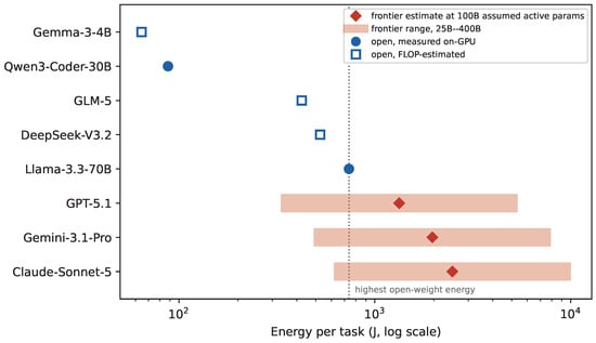
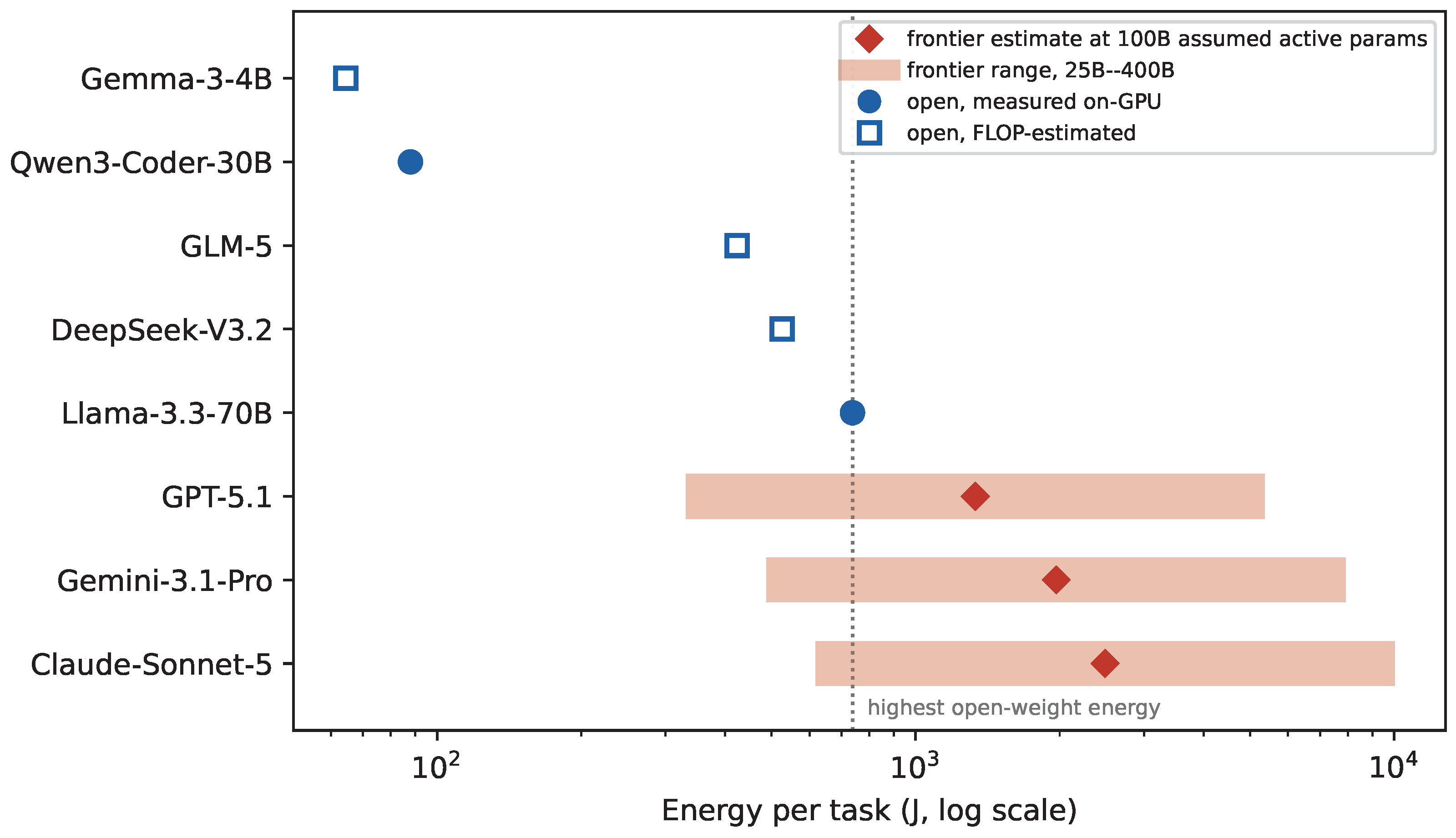
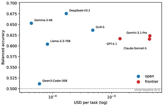
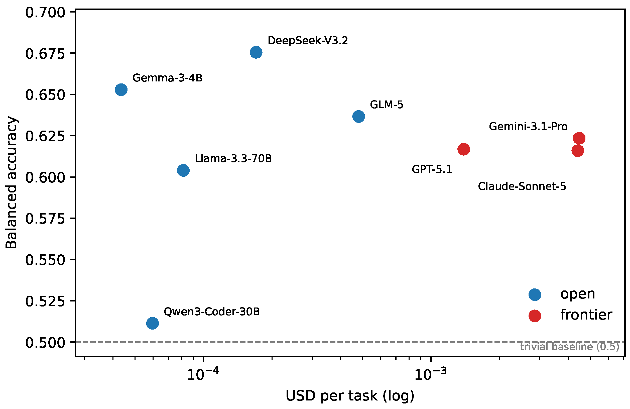
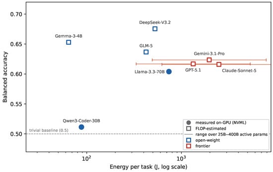
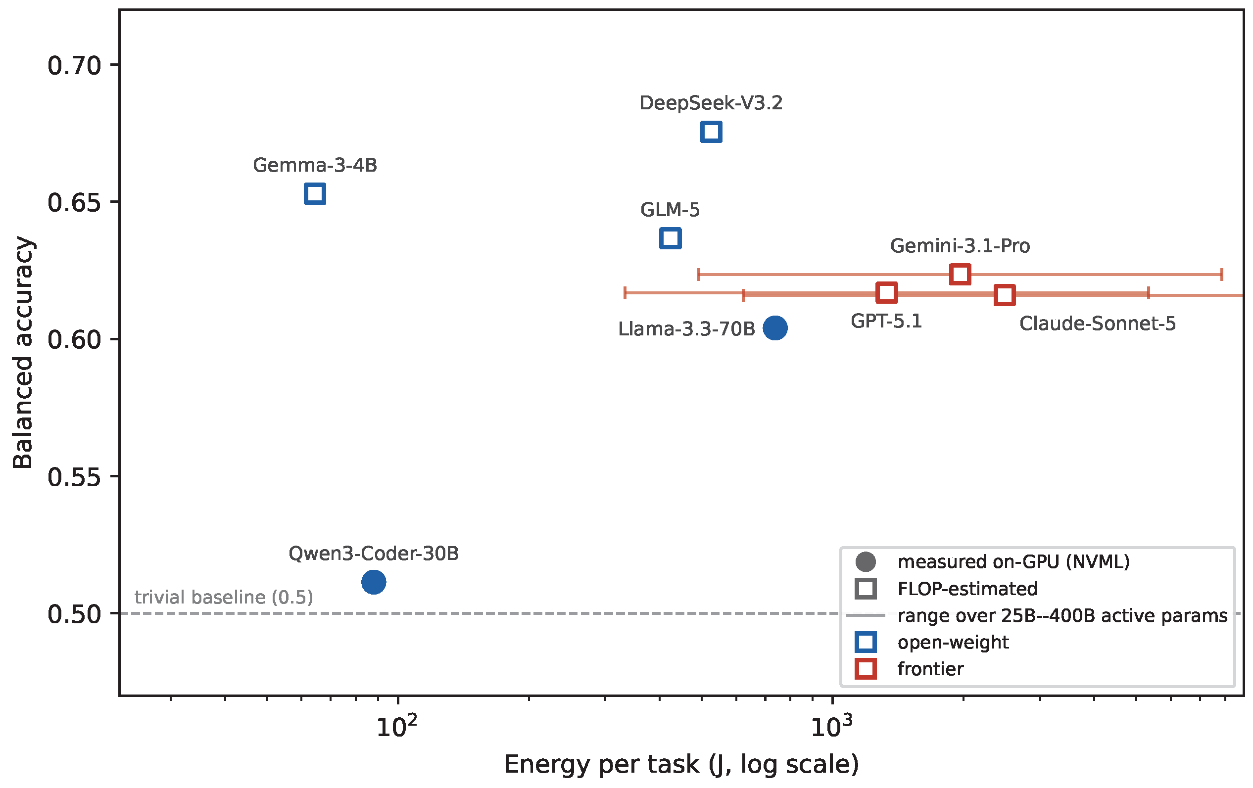

Disclaimer/Publisher’s Note: The statements, opinions and data contained in all publications are solely those of the individual author(s) and contributor(s) and not of MDPI and/or the editor(s). MDPI and/or the editor(s) disclaim responsibility for any injury to people or property resulting from any ideas, methods, instructions or products referred to in the content. |
© 2026 by the authors. Licensee MDPI, Basel, Switzerland. This article is an open access article distributed under the terms and conditions of the Creative Commons Attribution (CC BY) license.