Abstract
Revision game is a very recent advance in dynamic game theory and it can be used to analyze the trading in the pre-opening stock market. In such games, players prepare actions that will be implemented at a given deadline, before which they may have opportunities to revise actions. For the first time, we study the role of the deadline in revision games, which is the core component that distinguishes revision games from classic games. We introduce the deadline distribution into revision game model and characterize the sufficient and necessary condition for players’ strategies to constitute an equilibrium. The equilibrium strategy with respect to the deadline uncertainty is given by a simple differential equation set. Governed by this differential equation set, players initially fully cooperate, and the cooperation level decreases as time progresses. The uncertainty has a great impact on players’ behavior. As the uncertainty increases, players become more risk averse, in the sense that they prefer lower mutual cooperation rate rather than higher payoff with higher uncertainty. Specifically, they will not stay in full cooperation for a long time, while after they deviate from the full cooperation, they adjust their plans more slowly and cautiously. The deadline uncertainty can improve the competition and avoid collusion in games, which could be utilized for auction design and pre-opening stock market regulations.
1. Introduction
Revision game [1] is a multiplayer continuous-time game with continuous action space. It starts at time and ends at a fixed deadline time 0. Players can prepare an initial action at time and thereafter revise their action according to a Poisson process, which is called revision opportunity. During the game, players can fully observe each other’s action. When a revision opportunity arrives, players can change their actions simultaneously. While players can change their actions many times, the payoff is only obtained at the deadline, which depends on the last action players choose.
Some work explores general properties of revision games. When players do not act simultaneously, Moroni et al. propose asynchronous revision games and prove the existence of trembling hand and sequential equilibrium [2]. The use of asynchronous revision game in common and opposing game is studied by [3]. Stochastic revision game is defined by [4] where players’ payoff not only depends on the last action, but also the environment state. They prove the existence of Markov perfect equilibrium. Gensbittel et al. study the equilibrium payoff revision game, which they call revision value, and characterize the equilibrium strategy for zero-sum revision games [5].
Many real-world scenarios can be modeled as revision games. A mostly well-studied case is the pre-opening phase in stock markets such as Nasdaq or Euronext. Traders can submit orders before the opening of the market, which can be changed until the opening time. The opening price is determined by submitted order price and quantity, which can be seen on the public screen. Another case is the online auction websites like eBay, where bidders actually play a revision game during the auction. The eBay auctions usually have a deadline, before which bidders can revise their bids many times. Bidders’ opportunities to use eBay and to change bids are following a stochastic process (many human activities can be characterized by a Poisson process). In [1], they apply revision game model into stock pre-opening period, where traders can revise orders based on the refreshment of public screen until market opens. They point out that traders may have incentive to revise their order over time during the pre-opening phase and form collusion. Although the result can not be interpreted as a precise description of the pre-opening phase, it provides possibility of implicit collusion among the market participants. Kamada and Sugaya also use revision game model to analyze candidates behaviors of election campaign. They explain why candidates use ambiguous language in campaigns and change their policies as the campaign progresses [6].
However, when players engage in games with a fixed deadline, there might be many problems. For example, a fixed deadline may lead to price manipulation [7]. Traders can profit from manipulating opening price by submitting large orders in the very last few seconds [8]. To tackle this realistic challenge, many exchanges, like Euronext, Deutshe Borse and Tel Aviv Stock Exchange, switched from opening trade that ends at a fixed time to one that ends at a random time [9]. Introducing uncertain deadline is also meaningful for online auction platforms such as eBay, where auctions usually have fixed deadlines [10]. Roth and Ockenfels find that there exist many late bids (called snipping), where some bidders may not bid until the last possible moment, thus reduce seller’s revenue [11]. Ockenfels and Roth show that snipping is sensitive to the rules of how auction ends [12]. Füllbrunn and Sadrieh conduct experiments about random-deadline auction and show that bidders in such auctions bid more frequently in the early stage than in fixed-deadline auctions [13]. Google also designs a patent of random ending time system for online auction so that bidders have no preferences over the time of bidding [14]. Häfner and Stewart show that by choosing appropriate ending time distribution it can mitigate front-running problem in a discrete blockchain auction [15].
In this work, we introduce the deadline distribution into revision game model and characterize the sufficient and necessary condition for players’ strategies to constitute an equilibrium, where the equilibrium strategy is given by a simple set of differential equation set. With theoretical analysis and experimental results on Cournot game and public goods game, we find that as deadline uncertainty increases, players will become less cooperative than in the fixed-deadline situation thus collusion can be controlled. Therefore, our work can be helpful in auction design and pre-opening stock market regulations.
2. Preliminaries
Consider a symmetric game with two players (our results easily extends to n-player case), where player i’ action and payoff are denoted by and , respectively. Players share the same action spaces A which is convex in . The game starts at time and ends at time 0. The ending time is called deadline. Players prepare an initial action at time and can revise actions when revision opportunities arrive during time interval . Revision opportunities’ arrival is based on a Poisson process with arrival rate . Players can fully observe the opponents’ initial action and subsequent revised actions. Players revise their actions according to revision opportunities simultaneously without any cost. There is only one payoff for each player, which is realized at the deadline. In this paper, we will analyze the symmetric equilibrium for this game, thus we denote players’ payoffs at a symmetric action profile as . We follow the following assumptions of revision games [1].
Assumption 1.
For each stage game at time , there exists a unique pure symmetric Nash equilibrium action profile , which is a where both players totally defect, and their payoffs ; there is also a unique optimal symmetric action profile and . If , is strictly increasing for (symmetrically holds if ).
Assumption 2.
Assume player i’s action and payoff are continuous and always exists. We denote player i’s maximum deviation gain at a symmetric action profile by . Moreover, is strictly increasing for (symmetrically holds if ).
Assumption 1 requires two distinct action profiles, one is Nash equilibrium action profile, the other is optimal action profile. The symmetric payoff monotonically decreases as we move away from the optimal action . Assumption 2 requires the continuity of players’ action and payoff, and define the maximum deviation gain. The deviation gain monotonically increase as we move away from the Nash equilibrium. The assumptions above are all very common in continuous action games, and can be found in some classic games such as continuous prisoner’s dilemma, the classic Cournot competition and the Bertrand competition.
3. Trigger Equilibrium for Fixed Deadline
The currently existing equilibrium strategy is a grim trigger strategy. By grim trigger, a revision game player initially follows her plan, but punishes the opponent if a certain level of defection (i.e., the trigger) is observed.
Denote t the remaining period until the deadline. At any time , a player’s continuation plan is function , which realizes an action a for each t. A plan decides an action a for each time point t. We say that action a is cooperative (or collusive) or achieves (some degree of) cooperation (or collusion) if it provides a higher payoff than the Nash equilibrium: .
A symmetric grim trigger strategy for revision games is defined as follows. Players start with the initial action , and when a revision opportunity arrives at time , they change their actions to . If any player fails to choose , which we regard that as betrayal, both players choose the Nash action in all future revision opportunities.
Next, we will characterize the set of trigger strategy equilibrium. Let be the arrival rate of a Poisson process. By this arrival rate, the probability of no Poisson arrival in the remaining time t is calculated as . The probability there is no future revision opportunity after t is . Therefore, the expected payoff of each player associated with strategy over period can be calculated as:
To form subgame-perfect equilibrium at time t, the incentive constraint for the trigger strategy with plan is:
The left side means that, if the player who deviates from the plan wants to realize the deviation gain, then no revision opportunity should arrive during . The right side says that, if there is one revision opportunity that arrives at time , the player who deviates from the plan gets the punishment . The incentive constraint shows that a player can not increase her payoff by deviating from . There are many that satisfy incentive constraint, so that many trigger strategy equilibrium exist.
The plan which satisfies the binding constraint of Equation (2) (i.e., the LHS is equal to the RHS) is called the trigger strategy equilibrium plan, or equilibrium plan. As time approaches the deadline 0, the RHS becomes zero. So the deviation gain on the LHS decreases as time goes by. This means the plan should be more uncooperative as the deadline approaches. When time is very close to the deadline, is near zero, so it must be that is close to the Nash equilibrium action . At the very deadline, we can know that: . Equation (3) is the condition for subgame-perfect equilibrium: no player can obtain excess payoff by deviating the plan at any time . By solving Equation (2), one can have the following Theorem 1.
Theorem 1.
Assume d is differentiable on and if (or symmetrically if ), then differentiating both sides of the binding incentive constraint of Equation (2) by t, we obtain a differential equation about the continuation plan x as:
with the boundary condition . Equation (3) gives the equilibrium plan for revision games with fixed deadline.
Note that this differential equation is a first-order ordinary differential equation, where is monotonically decreasing for (symmetrically holds if ). To solve it, we only need one boundary condition, which is . In summary, we can use the solution to Equation (3) with boundary condition as the trigger strategy in the fixed-deadline revision game. As long as every player obeys the trigger strategy, cooperation is achieved and everyone gets a higher payoff than Nash Equilibrium payoff.
4. Games with Bernoulli Deadline Distribution
In Section 3, the deadline (at time 0) is fixed and is common knowledge to every player. In this section, we will give the form of trigger strategy and equilibrium plan in the two-point random deadline situation.
4.1. Extended Revision Game
Consider a revision game where there are two possible deadlines, and the deadlines can be captured by binomial distribution. The scenario is depicted in Figure 1. The deadline is either time 0 with probability p or time with probability . Note that when players are in time period , they do not know when is the deadline time, only know the deadline probability distribution. But when they are at time , they will know the exact deadline time because the game either ends at time or continues. When the game continues, player know the deadline is not time , but time 0. As long as players pass through the time , the two-point deadline game suddenly transfers to the fixed deadline situation. For each case of the deadline, we can utilize the trigger strategy described in Section 3 to determine players’ plan.
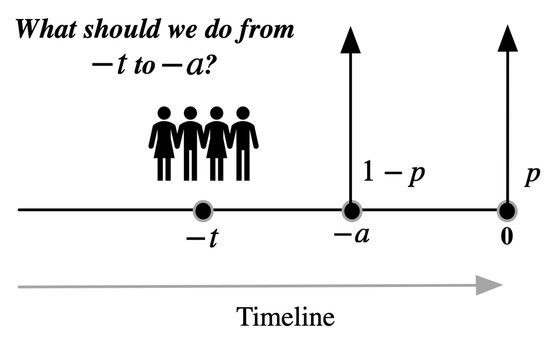
Figure 1.
Two possible deadlines, one is at 0 with probability p, and the other one is at with probability . Player makes a plan taking into consideration of both possible deadlines.
Therefore, by extending the LHS of Equation (2), the expectation of deviation gain at time in the two-point deadline situation can be written as follows.
The first term in Equation (4) is the expectation of deviation gain if the deadline is time 0, the second term is the expectation of deviation gain if the deadline is time .
Similarly, by extending the RHS of Equation (2), we can also rewrite the expectation of continuation punishment in the future as follows:
where the first integral is the punishment if the deadline is , while the second integral is that if the deadline is . It can be simplified into
This simplified form indicates, no matter when the deadline is realized, players will punish the deviation in the time period as long as there is a revision opportunity. But only if the deadline is time 0, they can take punishment measures in the time period . So the punishment from needs to multiply a probability factor p, while the punishment from does not need to.
4.2. Risk-Averse Equilibrium Plan
With Equation (4) denoting the expectation of deviation gain, and Equation (5) denoting the expectation of future punishment, we write the incentive constraint like Equation (2) to form the subgame perfect equilibrium in time period :
While there could be many trigger strategies which can satisfy Equation (6), we only focus on the strategy that can bring the player highest expected payoff.
Comparing Equation (2) and Equation (6), we can find that with deadline uncertainty introduced, the deviation gain in equation Equation (6) becomes larger than that in equation Equation (2), while the future punishment becomes smaller. This means with the deadline uncertainty, players get more temptation of deviation at time . Once deviated from the predetermined plan, the uncertainty of deadline can diminish the punishment harshness. Therefore, when players confronted with a more complex deadline rather than a fixed deadline, they will become less cooperative. Technically, the binding constraint of Equation (6) can give us the equilibrium plan in the following theorem.
Lemma 1.
For revision games with Bernoulli deadline distribution, the equilibrium plan on satisfying the binding constraint of Equation (6) is:
Proof.
Differentiating the LHS of Equation (6) by t, we can get
As for the RHS of Equation (6), notice that only the first item contains t, so we transfer the first item from the integral on to the difference between integral on and integral on . After differentiating by t, the RHS of Equation (6) becomes
Let the two differentials be equal, we can get Equation (7) as long as . □
Comparing Equation (7) with Equation (3), we can find that in the equilibrium plan for revision games with uncertain deadline, the players’ risk aversion is captured by the term
where the denominator is greater equal than 1. Thus the gradient for adjusting the plan becomes smaller, which indicates that even when confronting with one additional possible deadline, players become more conservative to adjust their actions. Thus we refer to the term in Equation (8) as the degree of risk aversion. As time point moves to time point 0, the denominator becomes closer to 1, which means as time goes by, players are more intent to go to a non-cooperative state. In the extreme case, if , then becomes 1 and Equation (7) degenerates to Equation (3). We will further interpret the meaning of the change in Section 4.2. It is worth noting that the Equation (7) only describes in which form the equilibrium strategy should be during the time period , but the exact solution to it can not be determined because of the lack of boundary condition. We will give the method of how to calculate the equilibrium strategy in Section 5.
5. Games with Multiple Deadline Distribution
The previous section investigates revision games with uncertain deadline in a simple Bernoulli distribution case as a warm-up, this section extends these games into an arbitrary deadline distribution cases.
5.1. Multiple Possible Deadlines
Consider a game with a set of multiple possible deadlines and the corresponding probability distribution . During time period , players can not be sure when the deadline will come. Similarly as in Equation (4), we can derive the expectation of deviation gain as follows.
Each term in Equation (9) represents one expected deviation gain for a possible deadline. For instance, for deadline , the value of denotes the probability no revision opportunity arrives during time period , while the deadline at time is realized with probability .
Similarly, we can derive the continuation punishment when someone deviates from the predetermined plan at time :
This summation depicts, if the deadline arrives at time , the one who deviates can only be punished in time period with probability . But, if the deadline arrives at time 0, the deviator has to suffer from the punishment all the way to time 0. The first item in Equation (10) represents the expectation of punishment in time period , the second item represents the expectation of punishment in time period , ⋯, the last item represents the expectation of punishment in period .
For plan x to constitute an equilibrium, it is required that
Equalizing and gives us the binding constraint for plan x together with them grim trigger mechanism to be an equilibrium strategy. According to the binding constraint, we easily get the following proposition.
Proposition 1.
When , the value of in Equation (10) is extremely small, by the binding constraint , it should be that , which further requires that at time 0 is the Nash action .
5.2. Equilibrium Plan as Differential Equation Set
To formally represent the equilibrium plan for any time, we do the following reasoning. Assume is the current time and let denote an arbitrary possible deadline. Let be the nearest possible deadline after time . That is, among all . On the one hand, for each , denote a cumulative distribution function (CDF) of the time distance by , which is the cumulative probability that no revision opportunity arrives during period . Therefore, the vector is a vector of CDFs. On the other hand, let denote the probability density function (PDF) of deadline at time .
We differentiate Equation (9) and the last term of Equation (10) which is correlated with variable t, and let the two result be equal, then we obtain the equilibrium plan for multiple possible deadline situation. The result is given as follows.
Theorem 2.
The equilibrium plan for revision games with multiple possible deadlines in the whole game period is characterized by a differential equation:
The value is the time-sensitive risk aversion rate and
where , , among all .
The corresponding discrete form of in Equation (13) is:
Comparing the two risk aversion rates in Equation (8) and in Equation (14), we can find that in the multiple possible deadline case, only the value of ra is different. Note that when or time points are close enough to time point 0, Equation (12) degenerates to Equation (3), i.e., the multiple possible deadline case degenerates to the fixed deadline case where the monotonicity of remains the same. As time approaches time 0, approaches .
Now we discuss about how to implement Theorem 2 and output the equilibrium plan x. Proposition 1 tells us that the final action at deadline should be the Nash action . Taking this fact as an terminal condition, we can apply Equation (12) recursively to get x for all . In the first loop of the recursion, we can obtain the first part of where by using and by introducing into Equation (13). Then we can know the agents’ action at time , which is a new seed for us to generate the second part of for . Repeat this operation for all , we can generate every part of the equilibrium plan x.
When recursively implementing Equation (12), the value of function g in Equation (13) could vary over time. This is because that as long as players pass through a possible deadline , it will be certain that this deadline sample didn’t materialize, meaning that the probability distribution (or equivalently, PDF g) over the remaining possible deadlines is updated. This updating is by Bayes’ law as follows, where is the new probability belief over the rest deadline points.
Therefore, at different time point , different g further results in different risk aversion rate , which finally affects the gradient of plan x at each time point .
5.3. Risk Aversion Rate in Equilibrium
Theorem 2 characterizes agents’ behavior in the equilibrium of general revision games with multiple possible deadlines. The equilibrium plan is given in a simple form as a differential equation, where the risk aversion rate quantifies how players handle the deadline uncertainty, and this uncertainty is time-sensitive. The risk aversion rate is correlated to the CDF of the Poisson arrival rate, the PDF of the deadline distribution, as well as the current time and the nearest possible deadline . Basically, it has the following features.
Proposition 2.
The risk aversion raterais bounded in .
Proof.
We only need to check the range of the denominator of the first line in Equation (14). Note that and , so the denominator ranges in then ra ranges in . □
Proposition 3.
Proof.
According to the Poisson process with arrival rate , on the one hand, we can find that in Equation (13) the numerator is is simply “the probability of no revision opportunity comes from to deadline 0 for the revision games with a fixed deadline”. On the other hand, in the denominator, each term is the probability that no revision opportunity arrives from time to the k-th possible deadline , while each term in the second vector is the probability density of the k-th possible deadline. Therefore, the denominator as a whole denotes the “the probability of no revision opportunity comes from to the uncertain deadline for the revision games with multiple possible deadline”.
Theorem 3.
. The risk aversion raterais monotonically non-decreasing in time . . For a given time and a fixed density of possible deadline,rais monotonically decreasing as the deadline range expands.
Proof.
Assuming that players at , the time points ahead are and the corresponding deadline distribution is . After they pass through time point , they will update the belief of deadline probability on from to by Equation (15). Let , and multiply ra by , then the denominator of new ra changes from to . Consider the difference: If , when means that the possibility of the deadline arrives at time is zero, then the difference becomes zero and denominator doesn’t change as well as ra. If , we only need to check the sign of , which is This means that the denominator of ra becomes smaller and ra becomes larger as players pass through the deadline point. Thus, we can get two conclusions. Firstly, as players progress with time, ra is monotonically non-decreasing; Secondly, the wider range the distribution spans, the smaller ra becomes. □
The pattern of ra revealed in Theorem 3 is important. By point , now we can know and explain the underlying mechanism that, as time goes by, players decay to mutual betrayal (i.e., action profile ) faster and faster. By point , it can be seen that as the deadline uncertainty increases, players’ plan becomes more conservative, in the sense that they do not prefer to change actions much. Thus Equation (13) and Theorem 3 significantly quantify agents’ risk aversion and their behaviors regarding different levels of uncertainty of the games’ deadlines. Figure 2 shows example equilibrium plans which are computed by Theorem 2 and have features in Theorem 3. We have the following observations from Figure 2. (i) By introducing deadline uncertainty, players deviate from full cooperation earlier and become less cooperative in the rest time. Thus, setting an uncertain deadline can reduce collusion among players. (ii) As the coverage of possible deadlines increases, ra monotonically decreases. Thus, with a larger deadline coverage, players not only stay shorter in the full cooperation state, they also adjust their actions more slowly.
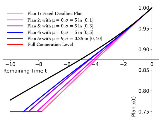
Figure 2.
Plans for Cournot game with various deadline distribution.
In a word, on the one hand, by utilizing Theorems 2 directly, we can derive the equilibrium plans. The solution of Equation (12) is essentially a generalized version of plans for players engaging in games with uncertain deadlines, and the existing plan derived in [1] is an extreme case of our result. On the other hand, by utilizing these results reversely, a mechanism designer can introduce the uncertain deadline into markets or auctions to reduce agents’ collusion and make the system better.
6. Experiments
We implement our theoretical results into the conventional Cournot duopoly game and public goods game.
6.1. Cournot Duopoly Game
There are two firms , whose production is denoted by . The payoff function for firm i is given by . Two firms can prepare an initial action at and revise their production amount according to a Poisson process until the unknown deadline. We set , . In the one-shot Cournot game, the full cooperation action is and the Nash action is 1, the corresponding payoffs are and 1, respectively. The revision Cournot game starts at time .
We introduce normal deadline distribution to our Cournot duopoly game. We change , of normal deadline distribution and Poisson process to check how these parameters affect the players’ behavior and payoff. We investigate the effects from four perspectives, the first is full cooperation duration as the red line depicted in Figure 2, the second is players’ average returns which represent producers’ payoff, the third is the Price of Anarchy (POA) [16] measuring the efficiency of this system, the fourth is consumers’ surplus [17] representing how much profits consumers can obtain from producers’ game. Red, blue and green colors in Figure 3 represent the coverage of deadline distribution, which are , and , respectively, and the corresponding is , , 5.
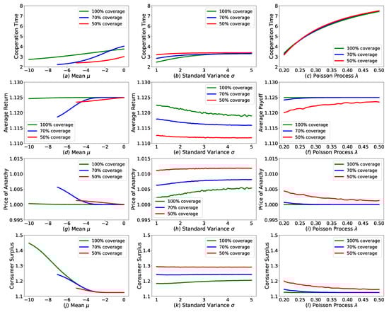
Figure 3.
Performances of equilibrium plan in revision Cournot game with various deadline uncertainty settings. For each column, we change , of normal deadline distribution and Poisson process , to check how these parameters affect the players’ behavior and payoff in each row.
(i) In the first column of Figure 3, we set , and change of normal distribution. We find that as approaches the starting time , the cooperation time and expected return decrease. We think that the movement of towards increases the chance that deadline arrives in a short time, thus producers choose to deviate full cooperation earlier and then obtain lower payoff, then the POA of this system becomes lower. As approaches the starting time , consumers can get more surplus because producers become less cooperative.
(ii) In the second column, we set , respectively, and check what ’s impact is. It shows that, when we increase of the normal distribution, cooperation time increases but the average payoff goes down. When given the plan, players’ payoff only depends on the last revision time. With bigger , probability that the deadline arrives at a position where is far away from increases, as well as the probability that the last revision opportunity arrives near time 0. When this happens, producers’ last action is approaching the Nash action, therefore the payoff decreases and the POA becomes higher. As producers’ profit decreases, the consumers’ surplus increases.
(iii) In the last column, we set , respectively, and increase Poisson from to . Doing so decreases the expectation of deviation gain in Equation (9) and increases the expectation of future punishment in Equation (10), thus makes cooperation time longer and return higher and reduces POA. This also decreases the consumers’ surplus due to the enforced cooperation between producers.
6.2. Public Goods Game
There are N players in our public goods game, where every player has money amount . We set the multiplication factor , which means that the money output is two times of the money input in the public pool. Then the total output is divided equally among each player no matter they donate or not. The Nash equilibrium of this game is that everyone donates nothing while the group’s total payoff is maximized when everyone donates everything(full cooperation). Players prepare an initial donation amount at time and revise the amount according to the Poisson process until the uncertain deadline arrives. The revision public goods game starts at time .
We introduce normal deadline distribution to our public goods game. We change player number N, , of normal deadline distribution and Poisson process to check how these parameters cause effects on the players’ behavior and payoff. Almost like in the Cournot duopoly game, we choose players’ full cooperation time, players’ average return and Price of Anarchy of the game as our observation indicators. Red, blue and green colors in Figure 4 represent the coverage of deadline distribution, which are , and , respectively, and the corresponding is , , 5.
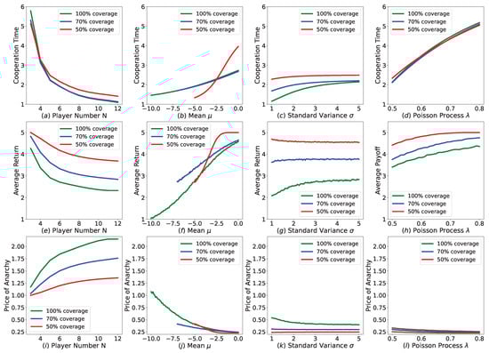
Figure 4.
Performances of equilibrium plan in revision public goods game with various player number and deadline uncertainty settings. For each column, we change player number N, , of normal deadline distribution and Poisson process , to check how these parameters cause effects on the players’ behavior and payoff in each row.
(i) In the first column of Figure 4, we set , and , and range player number from 3 to 12. We can see that as the player number increases, players will be less cooperative and lower payoffs will be obtained. Meanwhile, POA increases along with player number’s increasing.
(ii) In the second column, we set , and player number . As ranges from time 0 to time , full cooperation time and players’ average return decreases and POA increases.
(iii) In the third column, we set , , , and range from 1 to 5. We find that as increases, full cooperation time increases as well as average return of [−10, 0] distribution coverage, while average return of [−7, 0] and [−5, 0] distribution coverage basically remains the same.
(iv) In the last column, we set , , and range Poisson process from to . We can see that as increases, cooperation time and average return both increases and POA decreases correspondingly.
7. Conclusions and Future Works
This work is the first to identify the subgame perfect equilibrium in revision games with uncertain deadline. Our derived equilibrium plan consists of a set of differential equations, each of which contains a risk averse rate. We find some properties about the risk averse rate ra, such as when players move with time, ra is monotonically non-decreasing; when deadline distribution expands, ra is monotonically decreasing. By introducing deadline uncertainty, players become less cooperative thus collusion can be controlled.
We must point out that, although many scenarios like pre-opening and online auction can be modeled as revision game, the equilibrium strategy proposed by [1] or this paper can only provide one possibility of the reality. Thus, there are more work to do in the future to make our strategy more robust and practical. We plan to set players’ payoff function differently [18] and characterize their behaviors in uncertain deadline situation. Moreover, when players can not fully observe other people’s action [19], how to maintain cooperation in revision game is a realistic problem.
Author Contributions
Original draft, Z.W.; Review and editing, D.H. Both authors contributed to the writing and editing of the manuscript. All authors have read and agreed to the published version of the manuscript.
Funding
This research received no external funding.
Data Availability Statement
Not applicable.
Acknowledgments
We would like to thank the referees for suggestions and comments that improved this paper and the academic editors for their work.
Conflicts of Interest
The authors declare no conflict of interest.
References
- Kamada, Y.; Kandori, M. Revision games. Econometrica 2020, 88, 1599–1630. [Google Scholar] [CrossRef]
- Moroni, S. Existence of Trembling Hand Perfect and Sequential Equilibrium in Games with Stochastic Timing of Moves; Working Paper Series 19/005; Department of Economics, University of Pittsburgh: Pittsburgh, PA, USA, 2018. [Google Scholar]
- Calcagno, R.; Kamada, Y.; Lovo, S.; Sugaya, T. Asynchronicity and coordination in common and opposing interest games. Theor. Econ. 2014, 9, 409–434. [Google Scholar] [CrossRef][Green Version]
- Lovo, S.; Tomala, T. Markov Perfect Equilibria in Stochastic Revision Games; HEC Paris Research Paper No. ECO/SCD-2015-1093; HEC Paris: Paris, France, 2015. [Google Scholar]
- Gensbittel, F.; Lovo, S.; Renault, J.; Tomala, T. Zero-sum revision games. Games Econ. Behav. 2018, 108, 504–522. [Google Scholar] [CrossRef]
- Kamada, Y.; Sugaya, T. Valence Candidates and Ambiguous Platforms in Policy Announcement Games; University of California Berkeley: Berkeley, CA, USA, 2014. [Google Scholar]
- Goldstein, I.; Guembel, A. Manipulation and the allocational role of prices. Rev. Econ. Stud. 2008, 75, 133–164. [Google Scholar] [CrossRef]
- Ni, S.X.; Pearson, N.D.; Poteshman, A.M. Stock price clustering on option expiration dates. J. Financ. Econ. 2005, 78, 49–87. [Google Scholar] [CrossRef]
- Hauser, S.; Kamara, A.; Shurki, I. The effects of randomizing the opening time on the performance of a stock market under stress. J. Financ. Mark. 2012, 15, 392–415. [Google Scholar] [CrossRef]
- Sailer, K. Searching the eBay Marketplace, CESifo Working Paper No. 1848. 2006. Available online: https://papers.ssrn.com/sol3/papers.cfm?abstract_id=949418 (accessed on 8 September 2022).
- Roth, A.E.; Ockenfels, A. Last-minute bidding and the rules for ending second-price auctions: Evidence from eBay and Amazon auctions on the Internet. Am. Econ. Rev. 2002, 92, 1093–1103. [Google Scholar] [CrossRef]
- Ockenfels, A.; Roth, A.E. Late and multiple bidding in second price Internet auctions: Theory and evidence concerning different rules for ending an auction. Games Econ. Behav. 2006, 55, 297–320. [Google Scholar] [CrossRef]
- Füllbrunn, S.; Sadrieh, A. Sudden termination auctions—An experimental study. J. Econ. Manag. Strategy 2012, 21, 519–540. [Google Scholar] [CrossRef]
- Megiddo, N. Smooth End of Auction on the Internet. U.S. Patent 6,665,649, 16 December 2003. [Google Scholar]
- Häfner, S.; Stewart, A. Blockchains, Front-Running, and Candle Auctions. Front-Running, and Candle Auctions (14 May 2021). 2021. Available online: https://papers.ssrn.com/sol3/papers.cfm?abstract_id=3846363 (accessed on 10 September 2022).
- Guo, X.; Yang, H. The price of anarchy of Cournot oligopoly. In Proceedings of the International Workshop on Internet and Network Economics, Hong Kong, China, 15–17 December 2005; pp. 246–257. [Google Scholar]
- Anderson, S.P.; Renault, R. Efficiency and surplus bounds in Cournot competition. J. Econ. Theory 2003, 113, 253–264. [Google Scholar] [CrossRef]
- Selton, R. Re-examination of the perfectlessness concept for equilibrium in extensive games’. Int. J. Game Theory 1975, 4, 22–25. [Google Scholar]
- Kreps, D.M.; Wilson, R. Reputation and imperfect information. J. Econ. Theory 1982, 27, 253–279. [Google Scholar] [CrossRef]


Publisher’s Note: MDPI stays neutral with regard to jurisdictional claims in published maps and institutional affiliations. |
© 2022 by the authors. Licensee MDPI, Basel, Switzerland. This article is an open access article distributed under the terms and conditions of the Creative Commons Attribution (CC BY) license (https://creativecommons.org/licenses/by/4.0/).