Article

Analysing the Photo-Physical Properties of Liquid Crystals

School of Physics and Astronomy, University of Leeds, Leeds LS2 9BW, UK
*
Author to whom correspondence should be addressed.
Crystals 2024, 14(4), 362; https://doi.org/10.3390/cryst14040362
Submission received: 15 March 2024 / Revised: 27 March 2024 / Accepted: 29 March 2024 / Published: 11 April 2024
(This article belongs to the Special Issue Liquid Crystal Research and Novel Applications in the 21st Century)

Abstract

:
Intrinsically fluorescent liquid crystals are highly sought after for a variety of applications. Most of the measurements of photo-physical properties of liquid crystals are made in dilute solutions, which is mainly due to the relative ease of both these measurements and the interpretation of data. The fluorescence spectra depend on a number of parameters including the concentration in liquid crystal solutions, the device geometry, and the mesophase in which the spectra have been measured. Working with neat, or concentrated, liquid crystal samples adds experimental complexities such as the inner filter effect (IFE), which affects the collection of data, interpretation of the results, and accuracy of the conclusions. In this paper, we present a systematic study of the photo-physical properties of both a model reference material, Nile red, and a nematic liquid crystal, 4-cyano-4′-pentylbiphenyl (5CB). The influence on the emission spectra of an increasing solute concentration is investigated and discussed. Moreover, a detailed investigation of the influence of the used device geometry, as well as the choice of appropriate data fitting methodologies, are presented.

1. Introduction

Thermotropic liquid crystals (LCs) have been used in many applications, such as the now ubiquitous LC displays (LCDs), as the LC director (bulk molecular orientation) can be controlled by external manipulation which, in turn, produces unique changes to the optical behaviour. In LCDs, by far the most successful application of LCs to date [1], an electric field is used to reorient the director in order to obtain optical contrast [2]. Similarly, intrinsically fluorescent LCs are desirable for many applications as their emission properties could be electrically controlled by reorientation of the LC director.
Fluorescence, in general, is the process of spontaneous emission of light by electronically excited species of an organic or inorganic material. To achieve fluorescence, various methods of electronic excitation can be used, including: light in photo-luminescence [3], an electric field in electro-luminescence [4], and ultrasound in sono-luminescence [5]. Applications of intrinsically fluorescent LCs are widespread and include polarised lasers [6,7], fluorescent LCD materials to replace the back-light component found in LCDs [8,9] and improve viewing angles [10], anisotropic organic light-emitting diodes [11,12], fluorescent LC gels for photonic applications [13,14], ink-jet print dyes [15], and 1D semiconductors [16].
The fluorescence emission from LCs has been studied previously. A number of these studies investigate cyano-biphenyl (CB)-based LCs. Through these studies, it has been identified that CB-based LCs form ’excimers’. An excimer is a transient complex formed between the same type of molecules, where one is in the ground state, while the other in the excited state [17]. Excimers are observed in CB materials both in solutions at higher concentrations (>100 mM) and in the neat form [18,19,20,21,22,23]. While LCs are often highly fluorescent in dilute solution, once they are concentrated, either due to the nature of the particular LC phase, or simply due to the increased solution concentration, excimer formation either red-shifts and alters the spectrum, or it quenches the emission entirely [24]. In neat LCs, excimers have been identified both in their LC and isotropic phases [19,21,22]. These excimers are typically found to be long-lived, and they have been suggested to be related to the anti-parallel pair formation that occurs in CB-based materials [23,25,26].
Understanding the photo-physical properties of LCs in solution, i.e., as single molecules isolated from neighbouring LC molecules, is an important precursor to understanding the photo-physical properties of neat LCs. As high-quality UV-Vis and photoluminescence spectrometers are relatively commonplace, making photo-physical measurements on LCs in solution is relatively straightforward. However, interpretation of the data can be more complex, and it is not clear that conclusions based on measurements of LCs in dilute solution apply to LCs used in the neat form. Furthermore, often when the fluorescence behaviour is studied for high concentration solutions and for neat LCs, either the contributions from the so-called inner-filter effect (IFE) (details in Section 2.2) are ignored, or not enough details are provided in the description of the experimental geometry to accurately interpret and understand the presented results. In CB-based LCs, often the IFE, and its contribution to measured emission and excitation spectra, has not been considered and discussed. We note that the shift in emission wavelength caused by the excimer formation is often large enough in CB-based LCs that correct conclusions have often been reached in spite of this oversight even though this is not always true.
To address these issues, this paper provides a systematic investigation of some key photo-physical properties of a cyanobiphenyl LC, 5CB, which is often used in the literature as a ‘standard’ nematic LC for such investigations. The photo-physical effects are first investigated using a standard fluorophore, Nile red, which does not show excimer formation unlike the cyanobiphenyl LCs. The results from Nile red are compared to corresponding results from 5CB. The paper establishes the effect of Nile red and 5CB concentrations (in solution) on the emission properties, and it explains how the IFE can alter the observed spectral concentration dependencies seen in both materials. The investigation of the emission and excitation spectra of Nile red also shows how such spectra can distort at high concentrations in sample geometries such as cuvettes. Even though Nile red does not undergo any changes to the ground state at the concentrations studied here, spectral distortions to the emission and excitation spectra of Nile red are still observed even at relatively low concentrations. We further evaluate the role of the measurement device geometry on the measured emission spectra, using results from front-facing (defined in detail in Section 2.2) measurements on LC cells, which significantly minimise spectral alterations due to the IFE. Finally, the influence of the applied analysis procedures such as fitting routines of the emission spectra, on the final results, are discussed in detail.

2. Theory

2.1. The Effect of Concentration

The quantum yield of a fluorophore, Φ F , is defined as the number of emitted photons relative to the number of absorbed photons. Mathematically, this can be written as
Φ F = 0 F λ ( λ F ) d λ F ,
where F λ ( λ F ) represents the probability that an absorbed photon is emitted at a specific wavelength, λ F [3]. The fluorescence intensity, I F , is thus simply proportional to F λ ( λ F ) and the number of photons absorbed by the fluorophore, I A ( λ E ). This means that the fluorescence intensity of a fluorophore can be written as
I F ( λ E , λ F ) = k F λ ( λ F ) I A ( λ E ) ,
where λ E and λ F denote the wavelength of excitation and emission, respectively, and k is a constant which includes various experimental contributions, such as the bandwidth of the monochromators and the optical configuration [3].
I A ( λ ) can be written as:
I A ( λ E ) = I 0 ( λ E ) I T ( λ E ) ,
where I T ( λ ) is the intensity transmitted through the sample. From the Beer–Lambert law, I T ( λ E ) can be written as:
I T ( λ E ) = I 0 ( λ E ) exp ( 2.3 ε ( λ E ) l c ) ,
where l is the path length through the sample, epsilon(symbol) is the molar absorption coefficient and c is the concentration of the fluorophore in solution. All three of the Equations (2)–(4) can be combined to give the following:
I F ( λ E , λ F ) = k F λ ( λ F ) I 0 ( λ E ) [ 1 exp ( 2.3 ε ( λ E ) l c ) ] .
The exponential can then be expanded to an infinite series for which the higher-order terms become negligible at low concentrations, allowing for further simplification:
I F ( λ E , λ F ) = 2.3 k F λ ( λ F ) I 0 ( λ E ) A ( λ E ) ,
where A ( λ E ) = ε ( λ E ) l c is the absorption at the excitation wavelength λ E (i.e., the Beer–Lambert law [27]). The final step is to integrate over the whole emission spectrum, which yields the following:
I F ( λ E ) = 2.3 k Φ F I 0 ( λ E ) A ( λ E ) .
This expression gives the fluorescence intensity as a function of parameters that are relatively simple to measure, except for k. Equation (7) shows that for lower concentrations, the fluorescence intensity of emission is directly proportional to the fluorophore concentration. However, expansion of the exponential concentration dependence ( I F ( λ E ) e c ) to a linear behaviour ( I F ( λ E ) c ) is only valid for low concentrations, and at some concentration, all of the incoming light will be absorbed by the fluorophore, leading to an upper-limit/saturation in fluorescence intensity. Equations (2) and (3) can be combined and then integrated over all emission wavelengths to give [28]:
I F ( λ E , c ) = k Φ F [ I 0 ( λ E ) I T ( λ E , c ) ] .
A clear implication of this is that when all the light is absorbed by the sample, i.e., I 0 ( λ E ) > > I T ( λ E ) , the effect of concentration on the emitted intensity is lost. By measuring the fluorescence intensity for increasing concentrations e.g., of LCs in solution, this behaviour is often not observed due to another effect called the inner filter effect [28].

2.2. The Inner Filter Effect (IFE)

Liquid crystals are generally optically very dense in their LC state due to high amounts of absorption and scattering, which makes them difficult to study in neat form using traditional fluorescence spectroscopy methods. The IFE is suggested to be the root cause for this [28,29]. The IFE has been suggested to be present at some level in almost all published emission measurements [30]. However, despite its almost universal appearance, it is often ignored in the literature, which can lead to incorrect and misleading conclusions; the IFE can both dramatically quench emission intensity and induce significant spectral distortions [28,29].
There are two key types of IFE: primary and secondary IFE. Primary IFE is a natural consequence of the sample absorbing light. As light travels through the sample, individual photons are absorbed before being emitted in a random direction, resulting in fewer photons reaching the measurement volume. If the concentration of absorbing species is high enough, almost no light will reach the measurement volume and the measured fluorescence intensity will be significantly reduced. Secondary IFE, sometimes known as secondary absorption, is where a photon emitted by the fluorophore is absorbed by another molecule and is then emitted in a random direction before it reaches the detector. This will induce significant spectral distortions due to lost photons. The smaller the overlap between the emission and absorption, or excitation peaks (the Stoke’s shift), the stronger the effect of secondary IFE becomes [29].
In the most commonly used experimental geometry for measuring fluorescence spectra, the sample is contained in a cuvette placed along the beam path, and the data are collected at a right angle (shown in Figure 1a). As both primary and secondary IFEs significantly influence experiments in this geometry, many suggestions to correct for these effects have been proposed [28,29,31,32]. However, these correction methods often require complicated experimental setups, significant time for data collection, and do not provide notable reduction in errors. Therefore, it has been suggested that front-face measurements (such as the one shown in Figure 1b) offer significant advantages over these other techniques; the front-face measurement geometry avoids the excitation and emission paths passing through the entire sample [33], which makes correcting for IFE simpler. It has recently been shown that it is extremely difficult to completely eliminate the IFE from any measurements, and the IFE can only be minimised by use of front-face measurements on thin-film samples [29]. Thus, importantly, the thin sandwich cells typically used to study many properties of LCs provide an ideal geometry for front-facing photo-physical studies.

3. Materials and Methods

All materials, including solvents, used in this study were purchased from the commercial supplier Sigma-Aldrich and used without further purification. Care was taken to only use spectroscopic grade solvents of the highest purity (>99.5% as rated by the manufacturer) since trace impurities are often fluorescent and so would be detectable in the measured emission and excitation spectra. The chemical structures of 9-(Diethylamino)-5H-benzo[a]phenoxazin-5-one (Nile red) and the liquid crystal used in this study, 4′-pentyl-[1,1′-biphenyl]-4-carbonitrile (5CB), are shown in Figure 2. The LC exhibits a nematic phase at room temperature and a nematic to isotropic phase transition at 35.5 °C. Both Nile red and 5CB are easily soluble at relatively high concentrations using standard solvents such as methanol.
The fluorescence experiments were carried out using an Edinburgh Instruments FLS1000 photoluminescence spectrometer equipped with dual monochromators on both the excitation and emission sections of the fluorimeter. An ozone-free xenon arc lamp was used to excite the samples. The slit bandgaps, which control the bandwidth of the emission and excitation, were set to values between 0.5 and 1 nm depending on the intensity of the sample. The values were kept consistent for each individual sample in order to allow for a direct comparison of intensities. For experiments involving a cuvette geometry, quartz cuvettes with a 1 cm path length were used for the solutions. A N-K02exd TE sample holder was used to hold the cuvettes within the spectrometer. All measurements using cuvettes were conducted using the right-angle geometry shown in Figure 1a.
In experiments where LC cells were used, the light was directed via optical fibres to a temperature-controlled hotstage (T95, Linkam Instruments). The hotstage was mounted in a reflection geometry, such that the excitation and subsequent collected emission light were normal to the LC director for samples in a planar aligned nematic LC cell. A schematic representation of this experimental geometry is provided in Figure 1c. The LC cells/devices used in this study were purchased from commercial suppliers (AWAT, Poland), and the cells were filled in the nematic phase of 5CB. Planar alignment is achieved using rubbed polyimides with the two substrates assembled in an anti-parallel arrangement. The alignment quality and phase transition temperatures in the cells were checked using polarised optical microscopy (POM) before being used. The glass substrates (with a glass thickness of ∼1 mm) cause an attenuation of the excitation beam and a slight distortion of the emission spectra at wavelengths below 350 nm. Beam attenuation reduces the overall emission intensity, and this will be wavelength independent. The soda-lime glass shows reduced transparency below 350 nm (≃20% at 320 nm), which in turn reduces the intensity of the emission spectra below 350 nm. These effects are consistent across all experiments conducted in LC cells and do not change as a function of temperature, cell gap or concentration; therefore, these effects could be ignored. Cells fabricated using quartz glass could be used instead if the investigated material requires access to wavelengths below 350 nm. For the materials used in this study, this was not necessary. All emission and excitation measurements were corrected for the optical efficiency of the optical components within the spectrometer, and for a variation in bulb intensity across the spectrum using the stock correction files provided by the spectrometer manufacturer, which includes the optical efficiency of the optical fibres.

4. Results and Discussion

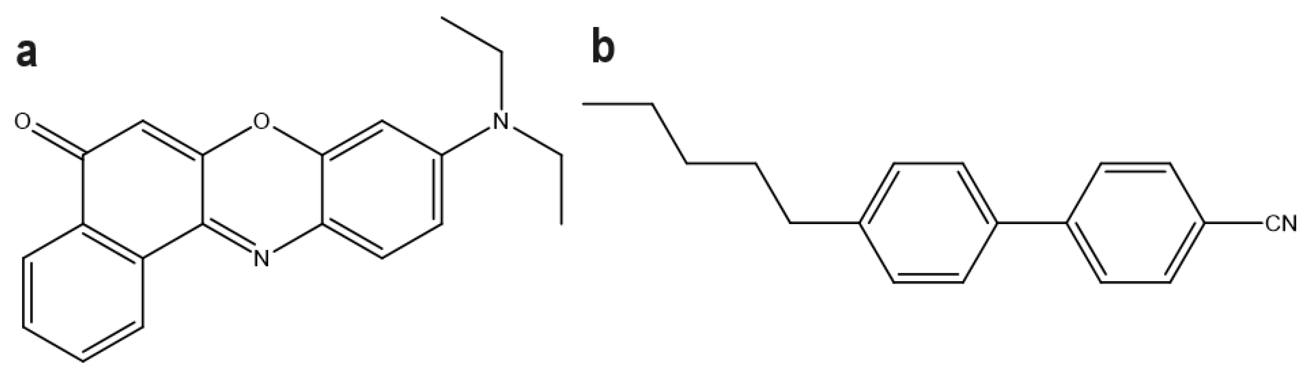
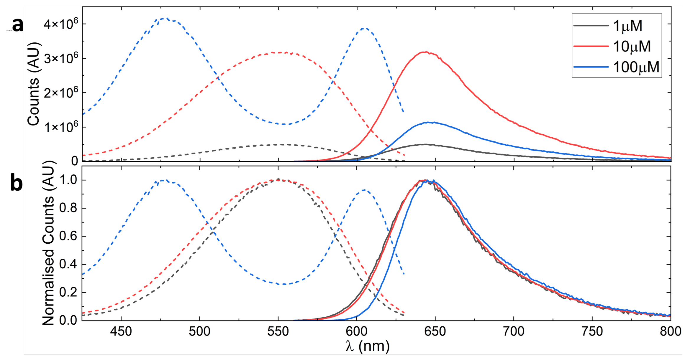
4.1. Nile Red—A Non Liquid Crystalline Fluorophore

Nile red is a commonly used dye [35,36] that can form H-aggregates (these are side-to-side parallel aggregates [37]) while in aqueous solution, which quenches the emission [38]. The dye does not undergo any changes in its photo-physical behaviour for the concentrations studied here in non-aqueous solutions such as methanol [36,39]. Typical excitation and emission spectra for three different concentrations of Nile red in methanol, recorded at 640 nm and 555 nm, respectively, are shown in Figure 3. From these graphs, it is clear that Nile red in 100 μM solution has a lower emission intensity than in the 10 μM solution. The normalised spectra also demonstrate that as the concentration of Nile red increases, the shape of the peak changes on the lower wavelength side.
Equation (7) shows a linear relationship between intensity and concentration though it should be noted that this equation is specifically only valid for low concentrations as discussed in Section 2.1, and the results here could be interpreted as a violation of that linear dependence. However, the lack of a linear relationship between intensity and concentration, and the variation in peak shape, can in fact be attributed to the IFE. As the primary IFE acts to absorb the excitation beam before it reaches the measurement volume, the observed reduction in emission intensity can be unrelated to any changes in material properties, such as quantum yield or intermolecular interactions. Similarly, the distortion in the emission shape profile is due to the secondary IFE, where the light that is emitted from the measurement volume is re-absorbed by Nile red molecules situated between the measurement volume and the detector. These photons are then re-emitted in random directions, which means that the chance of them being captured by the detector is low, and many of these photons are effectively lost [40].
The excitation spectra of Nile red also show effects of IFEs: both the lack of a linear concentration dependence of the peak intensity, and shape changes of the emission peaks are observed; the latter is most clearly observed for the 100 μM solution, where the single emission peak splits into two. The latter behaviour could be interpreted as a physical change in the ground state of the sample; however, we know for Nile red that this is not likely for these concentrations in this solvent. The more likely cause is primary IFE, where Nile red absorbs strongly at the investigated concentrations, thus preventing the excitation beam from reaching the measurement volume at its full strength, which reduces the emission intensity. Outside of the peak center, Nile red is less absorbent, and more incoming light can thus reach the measurement volume, resulting in artificial peaks at 480 nm and 605 nm.
The peak positions shown in the excitation spectra are thus determined from a balance between the increased intensity of the excitation source reaching the measurement volume and the reduced absorption coefficient of Nile red at these wavelengths. Spectral distortions due to IFE can be seen even at the relatively low concentrations of 10 μM where a slight increase in peak width can be seen when compared to the peak of the 1 μM solution.
Table 1 provides the intensity counts for the Nile red excitation peaks observed at different concentrations. The table shows that the intensity for the 550 nm emission peak at a concentration of 10 μM is 6.4 times the intensity of the 1 μM solution, even though a 10 times increase is expected based on a linear intensity vs. concentration. These non-linearities are reduced at the edges of the peak, where the absorption is reduced and hence also the effect of primary IFE. Excitation measurements at 450 nm, well away from the peak absorption, show the best agreement with the linear concentration vs. intensity dependence, even though the correlation is still not accurately following a linear behaviour.
Overall, the investigation of the emission and excitation spectra of Nile red shows the limitations of these types of measurements performed in cuvettes, especially at relatively high fluorophore concentrations. Even though Nile red does not undergo any changes to its ground state for the concentrations studied here [36,39], spectral distortions to the emission and excitation spectra are observed for concentrations even as low as 10 μM. While the concentration at which one begins to observe spectral distortions due to IFE changes from sample to sample (as demonstrated in the next section for 5CB), as shown from the work presented here, 10 μM is a commonly used dilute concentration. The presented results also show that the spectra, even for concentrations as low as 10 μM, are slightly distorted, which is a fact that must be considered when analysing the photo-physical measurements of liquid crystals.

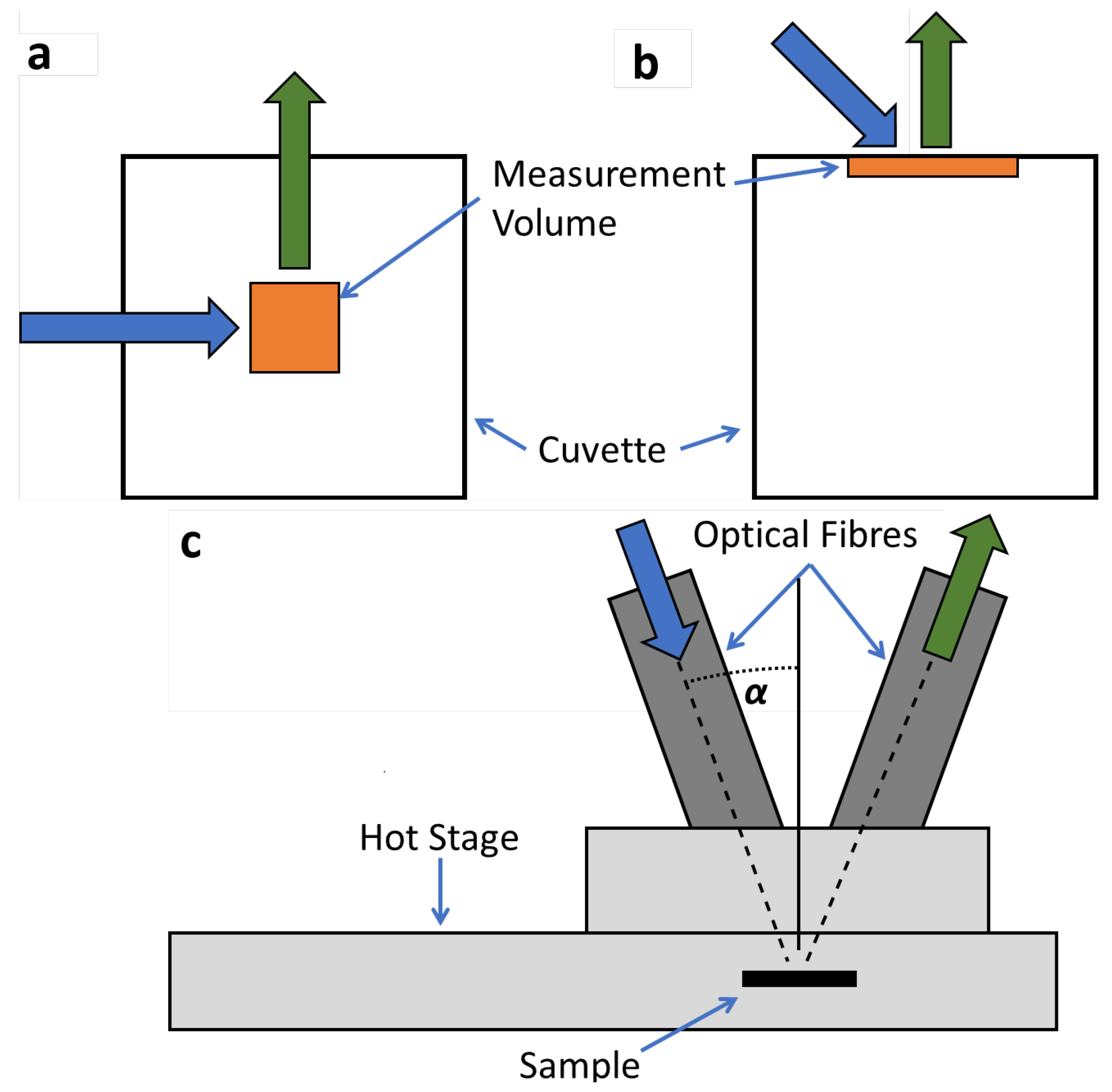
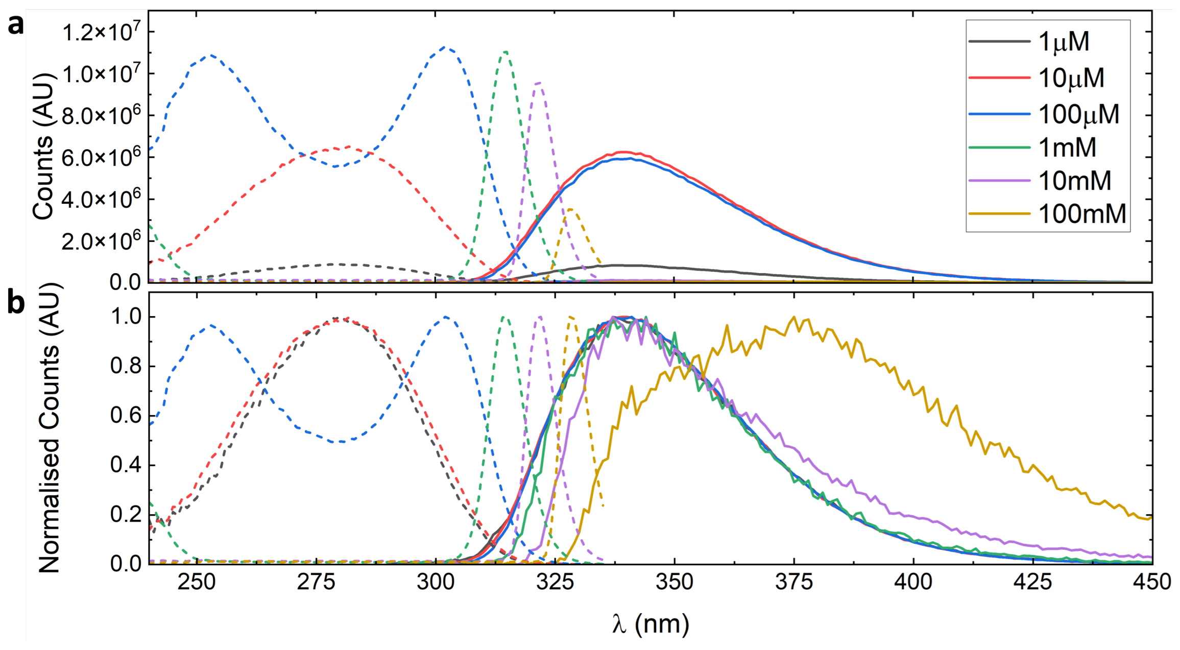
4.2. 5CB—Measurements Made in Cuvettes

Figure 4 shows the emission and excitation spectra of 5CB measured at 280 nm and 340 nm, respectively. Since 5CB is a nematic LC at room temperature, it is easily dispersed even at high concentrations using standard lab solvents such as methanol or acetone. This allows measurements of emission spectra up to concentrations as high as 100 mM. In the excitation spectra, the same splitting of the excitation peak that was seen for Nile red occurs also for 5CB at a concentration of 100 μM. As the concentration was increased further, the double peak increasingly separates until it becomes a single peak, which then continuously moves to longer wavelengths.
Similar to the behaviour of Nile red, the emission spectrum of 5CB does not follow a linear relationship over the investigated concentrations as we would expect from the simplified expression in Equation (7), although it should be noted that this equation is specifically only valid for low concentrations as discussed in Section 2.1. Spectral distortions are clearly visible, and the blue edge of the emission spectra red-shifts for increasing concentrations. 5CB has a smaller emission and excitation peak overlap compared to Nile red and is thus less affected by secondary IFE: concentrations as high as 1 mM are required for red-shifting to become visible, while for Nile red, red-shifting effects became visible at 10 μM. As mentioned before, we note that both the peak shape, the peak width, and the Stoke’s shift affects the overlap between the emission and excitation peaks of a given material and thus how much a particular material is affected by the IFE.
An additional effect that is present in 5CB, but does not occur in Nile red, is the formation and subsequent emission from excimers. The presence of excimer emission in liquid crystals has been proposed based on the emission measurements of highly concentrated solutions of LCs in isotropic solvents [19,20,21,22,23]. For example, the calamitic LC, 5CB, dissolved at low concentration (1.7 μM) in isopropyl alcohol (IPA) showed fluorescence emission at 335 nm, while at high concentrations (0.5 M), it instead showed a new emission peak at 380 nm but with a shoulder at 335 nm [21]. This red shift was attributed to excimer formation between anti-parallel (AP) pairs of 5CB molecules. These AP pairs are also known as ‘dimers’. Moreover, it has been shown that excimer formation in all nCBs and nOCBs is related to the same anti-parallel (AP) pair formation that is often stated as a ‘stabiliser’ for the LC phase [23,25,26]. However, although excimer emission for the nCB and nOCB series of LCs has been well studied [19,20,21,22,23,41,42,43,44], correct consideration to how the IFE may have affected those results has not always been given.
In Figure 4, for the high concentration samples (10 mM and 100 mM), an increase in the relative intensity can be seen near 400 nm. While some of this effect will be due to the secondary IFE, IFE-induced spectral distortions affect the lower wavelength side of the peaks more strongly and would be unlikely to be the cause of the big growth in emission at 375 nm for the 100 mM solutions. The main cause of this significant red-shift is more likely to be due to excimer formation, which for 5CB tends to happen in highly concentrated solutions. For the 100 mM sample, 5CB now emits more strongly at 375 nm than at the original peak position of 330 nm, which suggests that excimers appear to be the dominant emitting species. However, without being able to fully deconvolute the IFE and excimer induced red-shifts, it is difficult to conclude this for certain. Therefore, both better understanding excimer emission, and being able to effectively separate it from the primary and secondary IFE, is key to properly understanding the photo-physical properties of nCB liquid crystals.

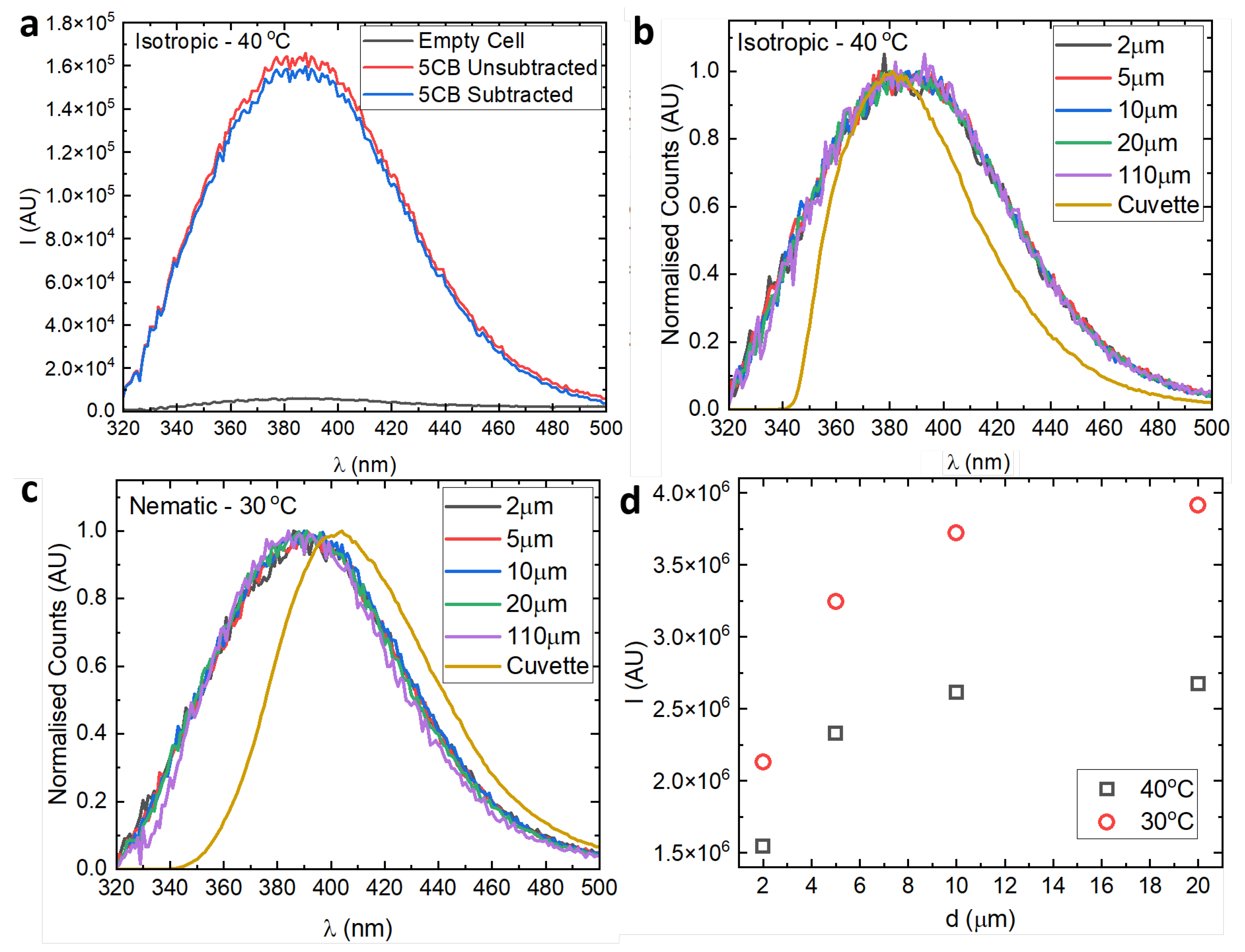
4.3. 5CB—Front-Facing Measurements

Measurements of 5CB in methanol at concentrations of 100 mM and comparisons with literature where excimer formation has been demonstrated in solutions of 5CB in IPA [21] demonstrate that excimers are present and that they influence the measured spectra. It is also clear that above a certain system-dependent concentration, the IFE is very strong in these optically dense systems, and this effect will be exacerbated for neat materials as the nematic phase will have considerably higher scattering due to director fluctuations and defect formation.
To minimise the IFE effects, measurements were performed in a front-facing geometry using LC cells, as discussed in Section 3. As described in Figure 1c, fibre optics are used both for the excitation light and for collecting the emission from the sample; the LC sample was contained in a LC cell and placed on a hot-stage connected to a temperature controller. The LC cells contained alignment layers on both the top and bottom substrates. These layers, and the rest of the LC cell assembly, induce a stable and weak spectral contribution; this contribution can be accurately removed by subtraction from the recorded data. This process is shown in Figure 5a. For 5CB, a relatively highly fluorescent fluorophore, the empty cell is not particularly significant; however, for very thin samples or samples with a lower fluorescence output, this step can become extremely important.
Figure 5b,c show the emission spectra of neat 5CB in its isotropic and nematic phases respectively, which were obtained using front-facing measurements in both LC cells and in a cuvette using the 90° angle method, respectively. The figure contains results from LC cells of different cell gaps, varying from 2 to 110 μm. These cells thus correspond to different optical path lengths for the excitation and emission beams. In both the isotropic and nematic LC phases, the IFE effects are minimised in the front-facing geometry compared with results from cuvettes. Therefore, the spectra presented here are highly accurate emission spectra of 5CB without experimental artefacts. A comparison of measurements from cells and cuvettes also demonstrates the magnitude of the IFE-induced spectral distortions in 5CB (both in the nematic and isotropic phases).
Overall, spectra for all of the investigated cell gaps, for 5CB in both its isotropic and nematic phase, show good agreement. This demonstrates that the resulting spectra remain largely unchanged even though thinner cells show significant surface anchoring effects, whereas for thicker cells (e.g., 110 μm), the anchoring effects are much less relevant. At 30 °C, in the nematic phase, a good agreement between different cells is observed for front-facing measurements. The spectra from the 110 μm cell show a slight change compared to the rest, which could be due an imperfect director alignment in the cell; this will increase scattering effects and slightly change the spectra. However, these distortions are negligible when compared to the significant differences between the spectra from cells and cuvettes, where different peak positions, and shapes, are observed for cells vs. cuvettes.
The comparison of results from cells and cuvettes shows the significance of correct consideration, and minimisation of the IFEs, in photo-physical studies. The effects of IFE could also be used to understand the penetration depth of incoming light in optically dense materials. We know that primary IFE attenuates the excitation light, which implies that the sample fluorescence only has contributions from before this sample-characteristic depth.
Figure 5c shows a plot of the overall intensity, defined as the numerically integrated area of the peak, as a function of the cell gap, for a 5CB LC in both its isotropic and nematic phases. It is clear that by 20 μm, the emitted intensity is significantly saturated, suggesting that the measurement can only study the sample to a depth of around 20 μm.

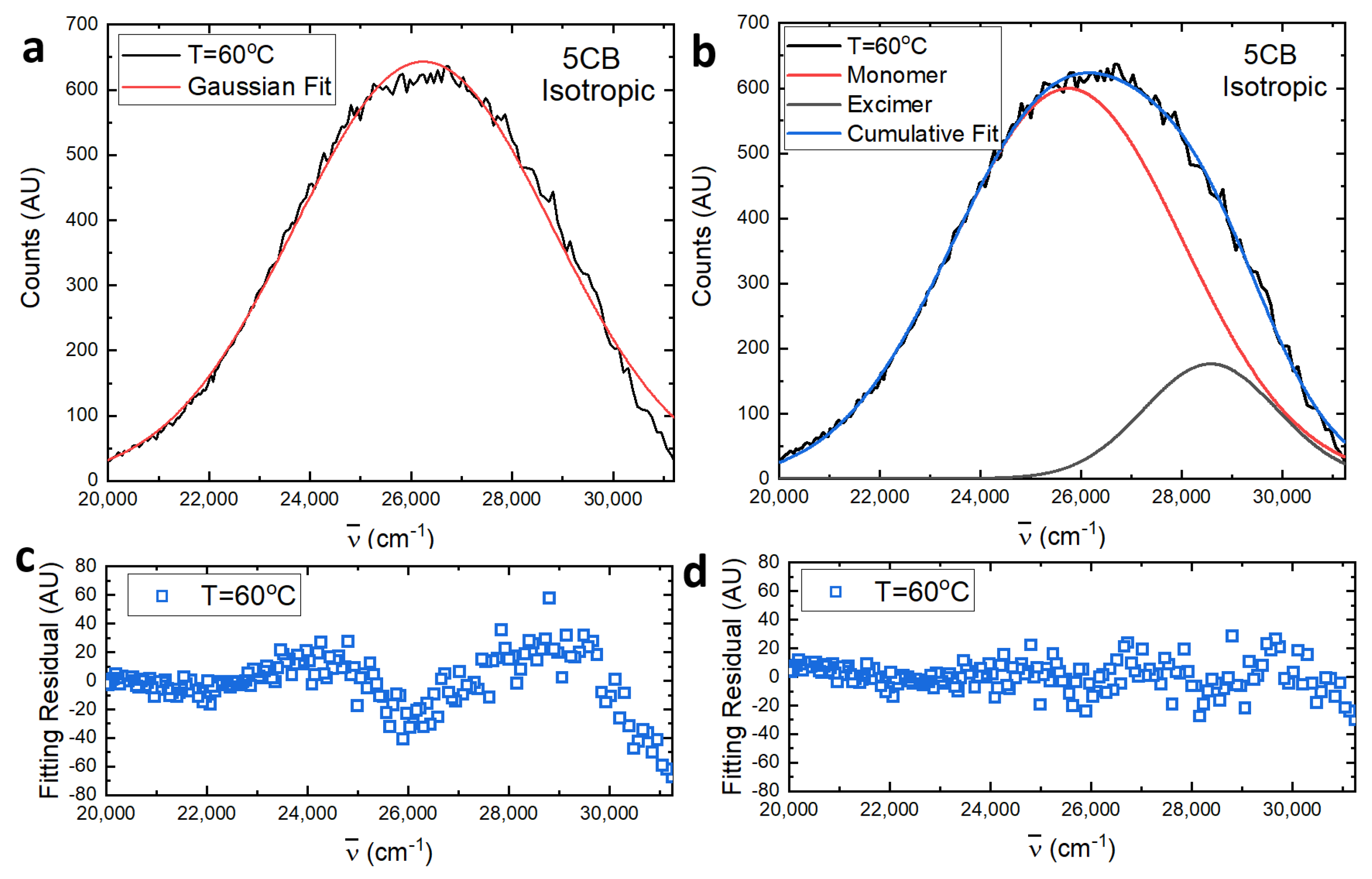
4.4. 5CB—Fitting the Emission Spectra

Once the emission spectra have been measured, a quantitative analysis can be conducted. Often, Gaussian peaks are used to fit fluorescence data [42,45,46,47,48,49], although sometimes other peak types [50] are being used. The fitting of peaks to the fluorescence spectra can be an important step and needs to be carried out correctly to reach correct conclusions on the physical origin of these spectra.
Spectrometers record photon counts per wavelength; however, processes that act to broaden emission spectra act on the energy scale, not on a wavelength scale. Furthermore, inhomogeneous broadening effects such as Doppler broadening [51] and the solvent ‘cage’ effect, where the variations in local environment leads to a statistical distribution [52], often result in the emission shape being Gaussian on an energy-based scale [53,54,55]. The wavelength is inversely proportional to energy; therefore, the y-axis conversion from intensity as a function of wavelength to intensity as a function of energy is not as simple as the x-axis conversion. Instead, a Jacobian conversion is required to convert the y-axis of the measured emission spectra. The conversion is needed before applying a fitting procedure using Gaussians [56].
Due to the inverse relationship between wavelength and energy, measurements evenly spaced on a wavelength scale will not be evenly spaced on an energy-scale. For example, a properly converted constant signal on a wavelength scale will not be constant on the energy scale; instead, the counts per unit energy is higher at lower energy/higher wavelength, resulting in a curved behaviour. The conversion has an even more significant effect on a Gaussian peak, and incorrectly fitting Gaussians on a wavelength-scale can thus lead to erroneous results. Figure 6 shows how three Gaussians, differing only in their peak positions, change shape when converted from wavenumber to wavelength scales. Peak 1 (black; left in Figure 6a) and right in Figure 6b) is significantly stretched in width and shrunk in height compared to peak 3 (blue; right in Figure 6a and left in Figure 6b). Note that all the Gaussians in the wavelength scale plot (Figure 6b) have been normalised relative to the tallest Gaussian, which has also been normalised to 1.
The Jacobian conversion is defined as
f ( E ) = f ( λ ) d λ d E ,
where E is the energy and λ is the wavelength, although E can be any quantity that is proportional to the energy. For the wavenumber-scale, this means that
f ( ν ¯ ) = f ( λ ) λ 2 ,
where ν ¯ is the wavenumber and
ν ¯ = 1 λ .
Once the data have been correctly converted, Gaussians can be fitted to obtain details about the spectra. A good general approach is to first perform a fit using only a single Gaussian, which is followed by checking the resulting fit residuals. If the fit residuals show only random noise, the Gaussian fit can be accepted. However, if the residual demonstrates a trend beyond random noise, an approach using a sum of multiple Gaussians can be attempted. The investigation of the residuals is repeated until a sufficiently good fit is obtained.
Figure 7 shows the emission spectrum of 5CB in its isotropic phase at 60 °C. The graphs show the results of fitting (a) one and (b) two Gaussians to the experimental spectra. For the single Gaussian fit, the residual contains a significant structure clearly not resulting from random noise. This is also clear from Figure 7a, which further confirms the inadequate quality of the fit. By adding a second Gaussian, the structure in the residuals is significantly decreased, and a good agreement between the fit and the data are observed, as shown in Figure 7b. For 5CB, the dual Gaussians correspond to ‘monomer’ emission and ‘excimer’ emission for the high wavenumber (lower wavelength) and low wavenumber (high wavelength) peaks, respectively. For the cuvette measurements, only a small emission shoulder at 350 nm (28,600 cm−1) is observed for the monomer contribution (Figure 4 100 mM), suggesting that the excimer emission is the dominant contribution. However, due to the dominance of IFE, this is difficult to conclude with certainty. Using front-facing measurements, the IFE can be significantly reduced, and hence it can be concluded with certainty that the excimer emission is the dominant contribution even at 60 °C, which is 25 °C above the transition to the nematic phase. Since excimer formation has been linked to AP pair formation in cyanobiphenyl liquid crystals [23], from front-facing experimental results, it is clear that the AP pair formation occurs far from the nematic phase, which is in agreement with the measurements made using dielectric spectroscopy on these liquid crystals [57].
The approach discussed here can be applied to the emission spectra of materials in general, and even though the interpretation of the physical/molecular origin of each fitted Gaussian is not necessarily trivial, performed correctly, this simple analysis can allow for a deeper understanding of the photo-physical properties of materials [58].

5. Conclusions

Fluorescent LCs are highly desirable for a wide variety of applications. However, measuring, understanding, and interpreting their photo-physical properties can be difficult due to secondary effects such as the IFE. Both highly concentrated LC solutions, and neat LCs, are optically highly dense and even though IFEs are present in almost all photo-physical measurements, they are exacerbated in optically dense media. This paper provides a systematic investigation of how IFEs can manifest in the fluorescence data. We illustrate the effects for two classes of materials, using (i) the fluorophore, Nile red, which does not show any spectral changes due to aggregation/collective behaviour for the solvents used here, and (ii) the liquid crystal, 5CB, which shows excimer formation at high concentrations and in neat solutions. The influences of solute concentration and optical path length on the results and the interpretations are discussed in detail. We demonstrate that by using front-face measurements, spectral distortions can be minimised, resulting in highly accurate emission spectra. Once, accurate spectra are obtained, the Jacobian wavelength-to-energy conversion should be used for correct descriptions of the peak behaviour; this procedure is illustrated using a sum of two Gaussians to describe the monomer and the excimer emission contributions, respectively, for 5CB.

Author Contributions

Conceptualisation, J.H. and M.N.; methodology, J.H.; software, J.H.; validation, J.H., J.M. and M.N.; formal analysis, J.H.; investigation, J.H., J.M. and M.N.; resources, M.N.; data curation, J.H.; writing—original draft preparation, J.H. and M.N.; writing—review and editing, J.H., J.M. and M.N.; visualisation J.H.; supervision, J.M. and M.N.; project administration, J.M. and M.N.; funding acquisition, J.M. and M.N. All authors have read and agreed to the published version of the manuscript.

Funding

This research was funded by the Engineering and Physical Sciences Research Council (EPSRC) funded Centre for Doctoral Training in Soft Matter and Functional Interfaces (grant EP/L015536/1).

Data Availability Statement

The data in this paper are available in the Leeds Data Repository (https://doi.org/10.5518/1500).

Conflicts of Interest

The authors declare no conflicts of interest. The funders had no role in the design of the study; in the collection, analyses, or interpretation of data; in the writing of the manuscript; or in the decision to publish the results.

References

  1. Jones, J.C. The fiftieth anniversary of the liquid crystal display. Liq. Cryst. Today 2018, 27, 44–70. [Google Scholar] [CrossRef]
  2. Klasen-Memmer, M.; Hirschmann, H. Nematic Liquid Crystals for Display Applications. In Handbook of Liquid Crystals: Volume 3, 2nd ed.; Goodby, J., Collings, P., Kato, T., Tschierske, C., Gleeson, H., Raynes, P., Vill, V., Eds.; John Wiley & Sons, Ltd.: Hoboken, NJ, USA, 2014. [Google Scholar] [CrossRef]
  3. Valeur, B.; Berberan-Santos, M. Characteristics of Fluorescence Emission. In Molecular Fluorescence, 2nd ed.; John Wiley & Sons, Ltd.: Hoboken, NJ, USA, 2012; pp. 53–74. [Google Scholar]
  4. Mitschke, U.; Bäuerle, P. The electroluminescence of organic materials. J. Mater. Chem. 2000, 10, 1471–1507. [Google Scholar] [CrossRef]
  5. Brenner, M.P.; Hilgenfeldt, S.; Lohse, D. Single-bubble sonoluminescence. Rev. Mod. Phys. 2002, 74, 425–484. [Google Scholar] [CrossRef]
  6. Bertolotti, M.; Sansoni, G.; Scudieri, F. Dye laser emission in liquid crystal hosts. Appl. Opt. 1979, 18, 528–531. [Google Scholar] [CrossRef]
  7. Mysliwiec, J.; Szukalska, A.; Szukalski, A.; Sznitko, L. Liquid crystal lasers: The last decade and the future. Nanophotonics 2021, 10, 2309–2346. [Google Scholar] [CrossRef]
  8. Grell, M.; Bradley, D.D.C.; Inbasekaran, M.; Woo, E.P. A glass-forming conjugated main-chain liquid crystal polymer for polarized electroluminescence applications. Adv. Mater. 1997, 9, 798–802. [Google Scholar] [CrossRef]
  9. Grell, M.; Bradley, D.D.C. Polarized Luminescence from Oriented Molecular Materials. Adv. Mater. 1999, 11, 895–905. [Google Scholar] [CrossRef]
  10. van Ewyk, R.; O’Connor, I.; Mosley, A.; Cuddy, A.; Hilsum, C.; Blackburn, C.; Griffiths, J.; Jones, F. Anisotropic fluorophors for liquid crystal displays. Displays 1986, 7, 155–160. [Google Scholar] [CrossRef]
  11. O’Neill, M.; Kelly, S. Liquid Crystals for Charge Transport, Luminescence, and Photonics. Adv. Mater. 2003, 15, 1135–1146. [Google Scholar] [CrossRef]
  12. De, J.; Abdul Haseeb, M.M.; Yadav, R.A.K.; Gupta, S.P.; Bala, I.; Chawla, P.; Kesavan, K.K.; Jou, J.H.; Pal, S.K. AIE-active mechanoluminescent discotic liquid crystals for applications in OLEDs and bio-imaging. Chem. Commun. 2020, 56, 14279–14282. [Google Scholar] [CrossRef]
  13. Tong, X.; Zhao, Y.; An, B.K.; Park, S.Y. Fluorescent Liquid-Crystal Gels with Electrically Switchable Photoluminescence. Adv. Funct. Mater. 2006, 16, 1799–1804. [Google Scholar] [CrossRef]
  14. Bobrovsky, A.; Shibaev, V.; Hamplová, V.; Novotna, V.; Kašpar, M. Photochromic and fluorescent LC gels based on a bent-shaped azobenzene-containing gelator. RSC Adv. 2015, 5, 56891–56895. [Google Scholar] [CrossRef]
  15. Zhang, L.; Cui, Y.; Wang, Q.; Zhou, H.; Wang, H.; Li, Y.; Yang, Z.; Cao, H.; Wang, D.; He, W. Spatial Patterning of Fluorescent Liquid Crystal Ink Based on Inkjet Printing. Molecules 2022, 27, 5536. [Google Scholar] [CrossRef]
  16. Sergeyev, S.; Pisula, W.; Geerts, Y.H. Discotic liquid crystals: A new generation of organic semiconductors. Chem. Soc. Rev. 2007, 36, 1902–1929. [Google Scholar] [CrossRef]
  17. Birks, J.B. Excimers. Rep. Prog. Phys. 1975, 38, 903. [Google Scholar] [CrossRef]
  18. David, C.; Baeyens-volant, D. Absorption and Fluorescence Spectra of 4-Cyanobiphenyl and 4-Alkyl- or 4-Alkoxy-Substituted Liquid Crystalline Derivatives. Mol. Cryst. Liq. Cryst. 1980, 59, 181–196. [Google Scholar] [CrossRef]
  19. Subramanian, R.; Patterson, L.; Levanon, H. Luminescence behavior as a probe for phase transitions and excimer formation in liquid crystals: Dodecylcyanobiphenyl. Chem. Phys. Lett. 1982, 93, 578–581. [Google Scholar] [CrossRef]
  20. Tamai, N.; Yamazaki, I.; Masuhara, H.; Mataga, N. Picosecond time-resolved fluorescence spectra of a liquid crystal: Fluorescence behavior related to phase transitions in cyanooctyloxybiphenyl. Chem. Phys. Lett. 1984, 104, 485–488. [Google Scholar] [CrossRef]
  21. Ikeda, T.; Kurihara, S.; Tazuke, S. Excimer formation kinetics in liquid-crystalline alkylcyanobiphenyls. J. Phys. Chem. 1990, 94, 6550–6555. [Google Scholar] [CrossRef]
  22. Ikeda, T.; Kurihara, S.; Tazuke, S. Persistence of ordering in 4-n-pentyl-4-cyanobiphenyl above the nematic-isotropic transition as detected by picosecond time-resolved fluorescence spectroscopy. Liq. Cryst. 1990, 7, 749–752. [Google Scholar] [CrossRef]
  23. Klock, A.; Rettig, W.; Hofkens, J.; van Damme, M.; De Schryver, F. Excited state relaxation channels of liquid-crystalline cyanobiphenyls and a ring-bridged model compound. Comparison of bulk and dilute solution properties. J. Photochem. Photobiol. A Chem. 1995, 85, 11–21. [Google Scholar] [CrossRef]
  24. Voskuhl, J.; Giese, M. Mesogens with aggregation-induced emission properties: Materials with a bright future. Aggregate 2022, 3, e124. [Google Scholar] [CrossRef]
  25. Goodby, J.W.; Davis, E.J.; Mandle, R.J.; Cowling, S.J. Nano-Segregation and Directed Self-Assembly in the Formation of Functional Liquid Crystals. Isr. J. Chem. 2012, 52, 863–880. [Google Scholar] [CrossRef]
  26. Dabrowski, R. From the discovery of the partially bilayer smectic A phase to blue phases in polar liquid crystals. Liq. Cryst. 2015, 42, 783–818. [Google Scholar] [CrossRef]
  27. Mayerhöfer, T.G.; Pahlow, S.; Popp, J. The Bouguer-Beer-Lambert Law: Shining Light on the Obscure. ChemPhysChem 2020, 21, 2029–2046. [Google Scholar] [CrossRef]
  28. Kimball, J.; Chavez, J.; Ceresa, L.; Kitchner, E.; Nurekeyev, Z.; Doan, H.; Szabelski, M.; Borejdo, J.; Gryczynski, I.; Gryczynski, Z. On the origin and correction for inner filter effects in fluorescence Part I: Primary inner filter effect - the proper approach for sample absorbance correction. Methods Appl. Fluoresc. 2020, 8, 033002. [Google Scholar] [CrossRef] [PubMed]
  29. Ceresa, L.; Kimball, J.; Chavez, J.; Kitchner, E.; Nurekeyev, Z.; Doan, H.; Borejdo, J.; Gryczynski, I.; Gryczynski, Z. On the origin and correction for inner filter effects in fluorescence. Part II: Secondary inner filter effect-the proper use of front-face configuration for highly absorbing and scattering samples. Methods Appl. Fluoresc. 2021, 9, 035005. [Google Scholar] [CrossRef] [PubMed]
  30. Bevilacqua, M.; Rinnan, A.; Lund, M.N. Investigating challenges with scattering and inner filter effects in front-face fluorescence by PARAFAC. J. Chemom. 2020, 34, e3286. [Google Scholar] [CrossRef]
  31. Fonin, A.V.; Sulatskaya, A.I.; Kuznetsova, I.M.; Turoverov, K.K. Fluorescence of Dyes in Solutions with High Absorbance. Inner Filter Effect Correction. PLoS ONE 2014, 9, 0103878. [Google Scholar] [CrossRef]
  32. Wang, T.; Zeng, L.H.; Li, D.L. A review on the methods for correcting the fluorescence inner-filter effect of fluorescence spectrum. Appl. Spectrosc. Rev. 2017, 52, 883–908. [Google Scholar] [CrossRef]
  33. Valeur, B.; Berberan-Santos, M. Steady-State Spectrofluorometry. In Molecular Fluorescence, 2nd ed.; John Wiley & Sons, Ltd.: Hoboken, NJ, USA, 2012; pp. 263–283. [Google Scholar] [CrossRef]
  34. Gryczynski, Z.K.; Gryczynski, I. Steady-State Fluorescence: Applications. In Practical Fluorescence Spectroscopy; CRC Press: Boca Raton, FL, USA, 2019; pp. 315–401. [Google Scholar]
  35. Jessop, P.G.; Jessop, D.A.; Fu, D.; Phan, L. Solvatochromic parameters for solvents of interest in green chemistry. Green Chem. 2012, 14, 1245–1259. [Google Scholar] [CrossRef]
  36. Martinez, V.; Henary, M. Nile Red and Nile Blue: Applications and Syntheses of Structural Analogues. Chem. A Eur. J. 2016, 22, 13764–13782. [Google Scholar] [CrossRef] [PubMed]
  37. Hestand, N.J.; Spano, F.C. Expanded Theory of H- and J-Molecular Aggregates: The Effects of Vibronic Coupling and Intermolecular Charge Transfer. Chem. Rev. 2018, 118, 7069–7163. [Google Scholar] [CrossRef]
  38. Ray, A.; Das, S.; Chattopadhyay, N. Aggregation of Nile Red in Water: Prevention through Encapsulation in β-Cyclodextrin. ACS Omega 2019, 4, 15–24. [Google Scholar] [CrossRef] [PubMed]
  39. Dutta, A.K.; Kamada, K.; Ohta, K. Spectroscopic studies of nile red in organic solvents and polymers. J. Photochem. Photobiol. A Chem. 1996, 93, 57–64. [Google Scholar] [CrossRef]
  40. Kuśba, J.; Grajek, H.; Gryczynski, I. Secondary emission influenced fluorescence decay of a homogeneous fluorophore solution. Methods Appl. Fluoresc. 2013, 2, 015001. [Google Scholar] [CrossRef]
  41. Abe, K.; Usami, A.; Ishida, K.; Fukushima, Y.; Shigenari, T. Dielectric and fluorescence study on phase transitions in liquid crystal 5CB and 8CB. J. Korean Phys. Soc. 2005, 46, 220–223. [Google Scholar]
  42. Bezrodna, T.; Melnyk, V.; Vorobjev, V.; Puchkovska, G. Low-temperature photoluminescence of 5CB liquid crystal. J. Lumin. 2010, 130, 1134–1141. [Google Scholar] [CrossRef]
  43. Klishevich, G.V.; Kurmei, N.D.; Melnik, V.I.; Tereshchenko, A.G. Temperature Dependence of the Luminescence Spectra of a 5CB Liquid Crystal and its Phase Transitions. J. Appl. Spectrosc. 2018, 85, 904–908. [Google Scholar] [CrossRef]
  44. Oladepo, S.A. Temperature-dependent fluorescence emission of 4-cyano-4-pentylbiphenyl and 4-cyano-4-hexylbiphenyl liquid crystals and their bulk phase transitions. J. Mol. Liq. 2021, 323, 114590. [Google Scholar] [CrossRef]
  45. Subhash, N.; Mohanan, C. Curve-fit analysis of chlorophyll fluorescence spectra: Application to nutrient stress detection in sunflower. Remote Sens. Environ. 1997, 60, 347–356. [Google Scholar] [CrossRef]
  46. Allabergenov, B.; Chung, S.H.; Jeong, S.M.; Kim, S.; Choi, B. Enhanced blue photoluminescence realized by copper diffusion doping of ZnO thin films. Opt. Mater. Express 2013, 3, 1733–1741. [Google Scholar] [CrossRef]
  47. Meira, M.; Quintella, C.M.; de O. Ribeiro, E.M.; Silva, W.L. Gaussian fit to the fluorescence spectra for determination of adulteration to diesel by addition of residual oil. Biomass Convers. Biorefinery 2015, 5, 295–297. [Google Scholar] [CrossRef]
  48. Ashenfelter, B.A.; Desireddy, A.; Yau, S.H.; Goodson, T.I.; Bigioni, T.P. Fluorescence from Molecular Silver Nanoparticles. J. Phys. Chem. C 2015, 119, 20728–20734. [Google Scholar] [CrossRef]
  49. Papagiorgis, P.; Stavrinadis, A.; Othonos, A.; Konstantatos, G.; Itskos, G. The Influence of Doping on the Optoelectronic Properties of PbS Colloidal Quantum Dot Solids. Sci. Rep. 2016, 6, 18735. [Google Scholar] [CrossRef]
  50. Bacalum, M.; Zorilă, B.; Radu, M. Fluorescence spectra decomposition by asymmetric functions: Laurdan spectrum revisited. Anal. Biochem. 2013, 440, 123–129. [Google Scholar] [CrossRef] [PubMed]
  51. Struve, W. Spectral Lineshapes and Oscillator Strengths. In Fundamentals of Molecular Spectroscopy; Wiley: Hoboken, NJ, USA, 1989; pp. 267–282. [Google Scholar]
  52. Wehry, E.L. Effects of Molecular Environment on Fluorescence and Phosphorescence. In Practical Fluorescence, 2nd ed.; Guilbault, G., Ed.; Modern Monographs in Analytical Chemistry, Taylor & Francis: Abingdon, UK, 1990; pp. 127–184. [Google Scholar]
  53. Valeur, B.; Berberan-Santos, M. Environmental Effects on Fluorescence Emission. In Molecular Fluorescence, 2nd ed.; John Wiley & Sons, Ltd.: Hoboken, NJ, USA, 2012; pp. 109–140. [Google Scholar]
  54. Kador, L. Stochastic theory of inhomogeneous spectroscopic line shapes reinvestigated. J. Chem. Phys. 1991, 95, 5574–5581. [Google Scholar] [CrossRef]
  55. Nemkovich, N.A.; Rubinov, A.N.; Tomin, V.I. Inhomogeneous Broadening of Electronic Spectra of Dye Molecules in Solutions. In Topics in Fluorescence Spectroscopy: Principles; Lakowicz, J.R., Ed.; Springer: Berlin/Heidelberg, Germany, 2002; pp. 367–428. [Google Scholar] [CrossRef]
  56. Mooney, J.; Kambhampati, P. Get the Basics Right: Jacobian Conversion of Wavelength and Energy Scales for Quantitative Analysis of Emission Spectra. J. Phys. Chem. Lett. 2013, 4, 3316–3318, Corrected in J. Phys. Chem. Lett. 2014, 5, 3497–3497. [Google Scholar] [CrossRef]
  57. Dalmolen, L.G.P.; Picken, S.J.; de Jong, A.F.; de Jeu, W.H. The order parameters 〈P2〉 and 〈P4〉 in nematic p-alkyl-p-cyano-biphenyls: Polarized Raman measurements and the influence of molecular association. J. Phys. 1985, 46, 1443–1449. [Google Scholar] [CrossRef]
  58. Dimitriev, O.P.; Piryatinski, Y.P.; Slominskii, Y.L. Excimer Emission in J-Aggregates. J. Phys. Chem. Lett. 2018, 9, 2138–2143. [Google Scholar] [CrossRef] [PubMed]
Figure 1. Schematic diagram of two commonly used sample geometries for fluorescence measurements. (a) Shows the most commonly found 90° geometry and (b) shows the alternative front-facing geometry, in cuvettes. (c) Schematic representation of the alternative geometry of measurement compatible with ‘standard’ LC cells, which allows for measurement of the emission properties of LCs as function of temperature, surface conditions etc. As the angle α is 20°, this can be considered as a front-face measurement [34]. In all figures, blue arrows indicates the direction of excitation, green arrow indicates the direction of observed emission and the orange area indicates the samples’ measurement volume.
Crystals 14 00362 g001
Figure 2. Chemical structures of (a) Nile red and (b) 5CB, the fluorescent materials used in this study.
Crystals 14 00362 g002
Figure 3. Excitation (dashed lines) and emission (solid lines) spectra of Nile red at various concentrations in methanol. The excitation and emission spectra were recorded at 640 nm and 555 nm, respectively. Shown on (a) is the raw spectra while on the (b) is the normalised spectra. The flattening of the excitation spectra of 10 μM and the subsequent splitting of the spectra into two peaks at 100 μM are due to the primary IFE. The normalised emission spectra show the effects of secondary IFE on its blue edge where there is some spectral distortion.
Crystals 14 00362 g003
Figure 4. Excitation (dashed lines) emission (solid lines) spectra of 5CB in various concentrations in methanol recorded at 340 nm and 280 nm, respectively. The raw spectra are shown in (a), and the normalised spectra is shown in (b).
Crystals 14 00362 g004
Figure 5. (a) Demonstration of the background subtraction process for 5CB at 40 °C. Emission spectra of neat 5CB liquid crystal at (b) 40 °C (isotropic phase) and (c) 30 °C (nematic phase). The results were obtained using front-face measurements in LC cells with various cell gaps. This is compared with the result obtained from neat 5CB in a cuvette of 1cm path length using the 90° angle method (orange solid line). (d) shows the cell gap dependence of emitted intensity, obtained by integrating the area under the emission spectra, for isotropic (black squares) and nematic phases (red circles).
Crystals 14 00362 g005
Figure 6. (a) Arbitrary Gaussian peaks with the same height and width parameters evenly spaced on a wavenumber scale. (b) The same arbitrary Gaussian peaks correctly converted to the wavelength scale showing how Gaussian-shaped spectra are asymmetrically stretched on the wavelength scale vs. the wavenumber.
Crystals 14 00362 g006
Figure 7. Results from fitting (a) a single Gaussian peak and (b) a double Gaussian peak to the emission spectra of 5CB in the isotropic phase using front-facing measurements. Figures (c,d) show the fitting residuals. Studying the fitting residuals here shows how a single Gaussian does not adequately describe the emission spectra of 5CB at this temperature.
Crystals 14 00362 g007
Table 1. List of intensity counts taken from the raw excitation spectra of Figure 3 for specific wavelengths for the three different concentrations of Nile red in methanol. The factors in brackets indicate the multiplication factor of the counts from their respective lower concentrations.
c (μM)450 nm500 nm550 nm600 nm
143,000254,100491,500169,000
10419,400 (9.7×)2,005,200 (7.9×)3,161,100 (6.4×)1,429,100 (8.5×)
1002,665,800 (6.4×)3,267,200 (1.6×)1,077,500 (0.34×)3,743,100 (2.6×)
Disclaimer/Publisher’s Note: The statements, opinions and data contained in all publications are solely those of the individual author(s) and contributor(s) and not of MDPI and/or the editor(s). MDPI and/or the editor(s) disclaim responsibility for any injury to people or property resulting from any ideas, methods, instructions or products referred to in the content.

