Abstract
The growth process of soybean plants needs a lot of water. The rapid detection of canopy wilting of soybean under drought stress is of great significance for soybean variety breeding, cultivation regulation and fine management. Aiming at the problems of cumbersome and time-consuming when the traditional chemical technology was used to determine soybean wilting index, a calculation method of wilting index for soybean canopy was proposed in this study based on multispectral images’ Fourier transform. Suinong 26, a northeast soybean variety, was taken as the object. First, four kinds of soybean multispectral images of green, red, red-edge and near-infrared channels were acquired by a Sequoia multispectral camera. Second, based on the multispectral reflection image preprocessed by median filter and mean filter, the target area of a multispectral image of the soybean canopy was extracted by the iterative threshold method and affine transformation algorithm, and the effective segmentation rate was 97.02%. In addition, Fourier transform was used to analyze the spectrum characteristics of the soybean canopy’s multispectral image. When the spectrum radius of each channel was 50, the energy reached more than 98% and was concentrated in the low-frequency region of the spectrum center. Finally, according to the difference between the low-frequency DC component and the proportion of total energy in the spectral radius of the multispectral images under normal and drought treatment, a calculation model of the soybean wilting index was constructed based on the energy spectrum of Fourier transform. The results showed that the difference of the wilting index between normal and drought treatment for the four channels (green, near-infrared, red and red-edge) was 2.38, 3.11, 3.56 and 4.11, respectively. The effectiveness of the wilting index was verified and analyzed by using the average leaf inclination angle. The determination coefficient R2 of the four channels between the calculated wilting index and the average leaf inclination angle was more than 0.85. This calculation method can provide a quantitative basis and technical support for the scientific regulation of ecological and morphological phenotypic traits of soybean plants under drought stress.
1. Introduction
Soybean is the main oil crop in the world, which provides important edible oil and high protein feed for humans and animals [1] and plays an important role in China’s national economy. The soybean plant has underdeveloped roots and large water demand for growth; thus, it is the most sensitive legume crop to water stress [2]. Drought will have a very serious impact on the soybean growth. China’s arid and water deficient areas account for 52.5% of the land area. The annual grain loss caused by drought is about 30 billion kg, accounting for about 60% of the total disaster loss [3]. It can be seen that drought stress does extremely serious harm to agricultural production and is the main environmental stress factor leading to crop yield reduction. Drought seriously affects the yield and quality of soybean. In severe years, drought will cause a loss in the soybean yield of about 40% [4]. Water shortage will seriously affect the morphology of the soybean plant [5]. When the soybean plant is subjected to drought stress, there will be a series of abnormal reactions, such as leaf wilting, withered yellow and short plant, which will cause plant death in serious cases [6]. Wilting is a phenomenon of drooping, shrinking or curling of young parts such as stems and leaves due to a water deficit and the inability of cells to maintain rigidity. It is a life feature of plants under drought stress, which is related to the expansion pressure in the plant cell wall [7]. It is an adaptive drought avoidance mechanism based on insufficient water absorption by the roots. Wilting reflects the water status within the plant and is the most widely used the index of plant drought stress [8]. The change of leaf wilting degree of a soybean is the external form of the comprehensive balance regulation between its internal water potential and complex production environment, which can directly and truly reflect the actual situation of water loss for soybean plants.
The research of domestic and foreign scholars on soybean wilting has mostly focused on physiology. For example, the research of Li et al. [9] focused on the physiological mechanism of soybean wilting resistance and pointed out that the degree of canopy wilting after drought stress was the external morphological expression of potential water, protection and regulation inside the plants, which can directly reflect the drought resistance of soybean. Wang et al. [10] observed and analyzed the morphological characteristics of soybean canopy and root system by controlling water to wilt soybean at the seedling stage and then evaluated the local varieties and excellent varieties. With the rapid development of measurement technology, digital equipment can be used to measure some phenotypic traits of plants [11,12,13]. Lama, et al. [14] obtained the multispectral image of rigid plants based on UAV and calculated leaf area index. Guimarães et al. [15] used UAV to obtain three-dimensional point cloud data of tree images, providing a feasible scheme for measuring and detecting complex forest structures in forestry applications. Mcglade et al. [16] used low-cost remote sensing technologies CRP and RGB-D to perform forest resources inventory tasks in forestry applications. Jalonen et al. [17] used terrestrial laser scanning (TLS) technology to study the physical characteristics of mixed floodplain vegetation and estimate the vertical distribution of woody vegetation. Sadeghifar et al. [18] tested the ability of the Artificial Neural Network (ANN), Adaptive Neuro-fuzzy Inference System (ANFIS), M5P and Random Forest (RF) soft-computing methods to predict the wave height of the Persian Gulf so as to obtain more accurate wave height prediction. The above technologies had broken through the limitations of traditional measurements and solved the problem of obtaining plant wilting phenotypic traits to a certain extent. Zhao et al. [19] used a 3D scanning device based on the principle of laser oblique range measurement to obtain the original information of zucchini leaf morphology and defined a leaf wilting index based on fractal dimension to quantitatively describe its wilting morphology. Zhang et al. [20] adopted a laser scanning device to obtain the leaf morphology, combined with different methods to define the wilting index to quantitatively describe plant wilting state and verified the applicability of using laser scanning device to obtain the leaf morphology through simulation experiments. Cai et al. [21] took zucchini as the research object and used 3D laser scanning technology to obtain plant leaf state information to calculate its wilting index by using Fourier transform so as to monitor the early wilting morphology of plants. Zheng et al. [22] used the non-contact laser scanning device to obtain the three-dimensional morphological information of plant leaves to quantitatively describe the plant wilting state and reflect the plant water deficit stress by measuring the body wilting characteristics of plant leaves. Zhang et al. [23] took cucumber and zucchini as experimental objects and used the TOF camera to obtain 3D image information of the plant leaf state to calculate their wilting index by Fourier transform in a discrete time domain. At present, there are few reports on the rapid and nondestructive determination of the soybean leaf wilting condition. Therefore, in order to avoid the shortcomings of cumbersome and time-consuming when using traditional chemical technology to evaluate plants’ wilting index, this paper applied multispectral image analysis technology, which had the advantages of low instrument cost, convenient detection and high image resolution [24], and carried out the research on the calculation method of the soybean canopy wilting index based on Fourier transform of the multispectral image. The multispectral image of the soybean canopy was obtained by a Parrot Sequoia multispectral camera (Parrot Drone SAS, Paris, France). Based on the canopy image, the amplitude frequency characteristics of the canopy’s multispectral image after Fourier transform were analyzed, and the calculation method of the soybean wilt index based on the energy distribution of the multispectral image was constructed, which provided a quantitative basis and technical support for the scientific regulation of ecological and morphological phenotypic traits of soybean plants under drought stress.
2. Materials and Methods
2.1. Experimental Materials
The soybean planting and acquisition of canopy information was carried out in Heilongjiang Bayi Agricultural University of Heilongjiang Province of China from 2017 to 2021. Under the outdoor conditions of 20~34 °C, the soybean variety of Suinong 26 was selected as the research object. The soybean variety was sensitive to light intensity, environmental temperature and soil moisture content. The change of the environment was easy to cause the shape change of plant leaves. The soybean seeds were sterilized and germinated after being selected and sown in the pot. The specific operation was as follows: first, the medium soil block was paved on the bottom of the polyvinyl chloride (PVC) material with a diameter of 30 cm and a height of 18 cm, and the screened fine soil without saline alkali was loaded until the weight of the pot was 5 kg. After emergence, set the seedlings of soybean to 3 plants in each pot when the seedlings grew to the V1 stage.
2.2. Acquisition Method of Experimental Data
The soybean multispectral acquisition system (Figure 1) was constructed by a Parrot Sequoia multispectral camera, combined with a homemade mobile acquisition rack, to obtain multispectral images of potted soybean plants. The camera can obtain four multispectral bands, including green (GRE), near-infrared (NIR), red (RED) and red-edge (REG) images. The corresponding wavelength ranges were 550 nm ± 40 nm, 790 ± 40 nm, 660 ± 40 nm and 735 ± 10 nm, respectively. In order to more clearly observe the characteristics of soybean wilting and ensure the integrity of the collected images, the experiment was taken in a vertical way, and the camera height was set to be 160 cm from the soybean canopy.
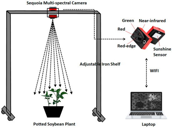
Figure 1.
Schematic diagram of the acquisition system for a soybean plant.
The experiment was divided into two treatments: normal water supply and drought treatment. The soybean plants were treated with water control from the V1 stage. The first data were collected from pot soybean at the V4 stage on the 15th day after water control, and the second data were collected at the V5 stage on the 20th day. Under the cultivation condition of normal water supply treatment, 30 groups of soybean multispectral images at V4 and V5 were collected, respectively. Under the cultivation condition of drought treatment, 30 groups of soybean multispectral images at V4 and V5 were collected, respectively, a total of 120 groups of experimental samples. In the study, four kinds of multispectral images of potted soybean were obtained through the acquisition system (Figure 2), and the above 120 groups of samples were used as the dataset for the calculation of soybean canopy wilting index in this paper.

Figure 2.
Original multispectral image of the soybean canopy: (a) GRE original image, (b) NIR original image, (c) RED original image, and (d) REG original image.
2.3. Overall Framework of Calculation Method of Wilting Index for Soybean Canopy
First, the soybean multispectral image was obtained by using the constructed soybean plant acquisition system, and the reflection image of soybean multispectral image was obtained by the empirical linear method. In order to improve the accuracy of image recognition, the median filter method and mean filter method were used to denoise the soybean reflection image. The soybean canopy was segmented by the iterative threshold method and canopy extraction algorithm based on affine transformation. The canopy characteristics were statistically analyzed by a gray histogram. Then, the soybean canopy was Fourier transformed, and the spectrum of the canopy was analyzed. According to the spectrum characteristics, the soybean wilting index based on the Fourier-transform energy spectrum was proposed. Finally, the wilting index of the four channels of soybean canopy multispectral image was calculated, and the effectiveness of the proposed wilting index in this paper was verified by the average leaf inclination. The overall framework of the calculation method of the wilting index for the soybean canopy was shown in Figure 3.

Figure 3.
Overall framework of the calculation method of the wilting index for the soybean canopy.
3. Calculation Method of Wilting Index for Soybean Canopy
3.1. Preprocessing of the Multispectral Image for Soybean Canopy
3.1.1. Acquisition of the Multispectral Reflection Image for Soybean Canopy
- Multispectral camera calibration
The lens of the multispectral camera was fixed vertically downward on the mobile data acquisition system. The standard grayscale plate (19.5 cm × 14.5 cm) with a reflectivity of 18% was taken as the target, and 20 groups of multispectral images of green, near-infrared, red and red-edge channels were obtained by using the multispectral camera with GPS mode. Then, the obtained multispectral images of the standard grayscale plate were imported into pix4d mapper software to complete the image mosaic, radiometric correction and orthophoto registration, and the reflection images of green, NIR, red and red-edge channels were obtained, respectively, which are shown in Figure 4.
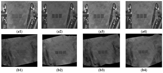
Figure 4.
Original multispectral image and reflection image: (a1) GRE original image, (a2) NIR original image, (a3) RED original image and (a4) REG original image; (b1) GRE reflection image, (b2) NIR reflection image, (b3) RED reflection image and (b4) REG reflection image.
According to the empirical linear method [25], the relationship was calibrated between the pixel value of the standard grayscale plate and its corresponding spectral reflection value in each channel after imaging. The least square method was used to solve the regression coefficients of the calibration equation of the multispectral camera, and the calibration equations of the green, NIR, red and red-edge channels of the multispectral camera were calculated (Table 1).

Table 1.
Calibration equation for the multispectral camera.
- 2.
- Acquisition of the multispectral reflection image for soybean canopy
The gray value distribution of the green, NIR, red and red-edge channels of the original multispectral image in Figure 2 was analyzed and calculated for the soybean canopy; the results are shown in Figure 5.
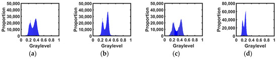
Figure 5.
Original multispectral images’ histogram of the soybean canopy: (a) GRE histogram, (b) NIR histogram, (c) RED histogram and (d) REG histogram.
Figure 5 showed that, in the original multispectral image of the soybean, the gray frequency distribution of green, NIR, red and red-edge channel was 0.1098~0.5255, 0.1176~0.8431, 0.1020~0.5686 and 0.0980~0.4667, reaching the peak at 0.3843, 0.3961, 0.4314 and 0.2510, respectively. The histogram was in a bimodal state, and the foreground features were clearly distinguished from the background.
According to the Sequoia calibration equation established in Table 1, the reflection image of the original multispectral image of soybean canopy was calculated. The green channel’s reflection image, near-infrared channel’s reflection image, red channel’s reflection image and red-edge channel’s reflection image of soybean canopy were obtained, respectively, and the corresponding gray histogram was analyzed; the results are shown in Figure 6.

Figure 6.
Soybean multispectral reflection image and corresponding histogram: (a1) GRE reflection image, (a2) NIR reflection image, (a3) RED reflection image and (a4) REG reflection image; (b1) GRE histogram, (b2) NIR histogram, (b3) RED histogram and (b4) REG histogram.
Figure 6 showed that, in the soybean multispectral reflection image, the gray frequency distribution of each channel was 0.0314~0.2706, 0~0.1567, 0~0.5137 and 0~0.7059, and its envelope line was basically consistent with the histogram trend of the original image. After the original multispectral image of soybeans was converted into a reflected image, the histograms of the four channels were shifted to the left by 0.1568, 0.2823, 0.1059 and 0.1412, respectively. The change of eigenvalues of the reflected image was basically consistent with the original image. Therefore, the multispectral reflected image was used to calculate the wilting index of the soybean canopy.
3.1.2. Denoising of the Multispectral Image for Soybean Canopy
In order to overcome the influence of noise in the process of image acquisition, the median filter and mean filter were used to denoise the multispectral image. A histogram statistical analysis was carried out to remove the influence of interference factors on canopy extraction. At the same time, the peak signal-to-noise ratio (PSNR), structural similarity (SSIM) and mean absolute error (MAE) were used as evaluation indexes to evaluate the quality of the denoising effect so as to select the optimal noise reduction processing method.
The basic principle of median filtering was to replace the central pixel value with the median value of all the pixels in a sliding filtering window [26]. If the gray value of the pixel with position in the image was , the pixel value of the point after median filtering was , which was expressed as:
where represented the set of pixels covered by the neighborhood template window centered on point , and represented the intermediate value of all values in a set.
According to the median filtering in Equation (1), a filtering window was selected to denoise the four channels of the multispectral image of soybean canopy, and the histogram was statistically analyzed (Figure 7).
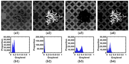
Figure 7.
Median filtering effect and corresponding histogram of the soybean multispectral image: (a1) GRE median filter, (a2) NIR median filter, (a3) RED median filter, (a4) REG median filter, (b1) GRE histogram, (b2) NIR histogram, (b3) RED histogram and (b4) REG histogram.
Figure 7 shows that, after median filtering of the soybean multispectral image, the average gray values of the green, near-infrared, red and red-edge channel histograms were 0.1505, 0.0392, 0.2441 and 0.1555, respectively, which were basically consistent with the average gray values of the original image. The NIR channel distribution was only 0~0.1569, and the frequency fluctuation was small.
The implementation process of mean filter was: in the sliding filter window, the central pixel value and other pixel values were averaged in the window, and then, this average value was used as the central pixel value of the filter output [27]. If the gray value of the pixel with position in the image was , then the pixel value of the point after mean filtering was , which was expressed as follows:
where was the side length of the block area, and was the neighborhood used for the calculation.
According to the mean filtering in Equation (2), a filtering window was selected to denoise the four channels of the soybean multispectral image, and the histogram was statistically analyzed (Figure 8).
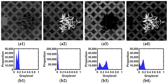
Figure 8.
Mean filtering effect and corresponding histogram of a multispectral image for the soybean canopy: (a1) GRE mean filter, (a2) NIR mean filter, (a3) RED mean filter, (a4) REG mean filter, (b1) GRE histogram, (b2) NIR histogram, (b3) RED histogram and (b4) REG histogram.
Figure 8 showed that, after the mean filtering of the soybean multispectral image, the average gray values of the histograms of each channel were 0.1506, 0.0392, 0.2429 and 0.1432, which were basically consistent with the average gray values of the original image. Among them, the histogram envelope line of the red and red-edge channels was relatively smooth, and the frequency fluctuation interval difference of the NIR channel was only 0.1569.
The noise reduction evaluation indexes of the multispectral images were all full reference image quality evaluation indexes [28], in which the PSNR calculation equation was as follows:
where and were the height and width of the image, respectively, was the original image, was the image to be evaluated and was the number of bits per pixel; the larger the value of was, the smaller the image distortion.
Since it was easy for human vision to extract the structural information from the image, the SSIM index was calculated to evaluate the similarity of the structural information of the two images. The equation was as follows:
where was the change of image brightness, was the change of image difference and was the change of image structure. The larger the value, the smaller the image distorted.
The MAE index can avoid the problem of error cancellation, so it can accurately reflect the actual prediction error. The MAE calculation Equation was as follows:
where, and were the height and width of the image, respectively, was the original image, was the image to be evaluated and was the number of bits per pixel. The smaller the value of , the smaller the image distorted.
Table 2 show that the average PSNR of multispectral images processed by the median filter and mean filter were 40.7570 and 39.5310, respectively, the average SSIM were 0.9333 and 0.9268, respectively, and the average MAE were 0.9678 and 1.1543, respectively. When denoising the multispectral image, the multispectral image processed by median filter was better than the mean filter in the PSNR, SSIM and MAE. It maintained detailed information such as the edge of multispectral image for soybean canopy and completely preserved the original information of the multispectral image. Therefore, the median filter method was used to filter and denoise the multispectral image for the soybean canopy.
Table 2.
Evaluation indexes of the multispectral image preprocessing.
3.2. Extraction of Soybean Canopy in the Multispectral Image
The background of the soybean multispectral images directly affected the calculation accuracy of the canopy wilt index. Extracting the effective region of the soybean canopy was a necessary prerequisite for accurate calculation of the canopy wilt index. Therefore, affine transformation was used to extract the soybean multispectral canopy image, which provided a real and reliable data source for calculating the soybean wilting index.
3.2.1. Selection of Standard Template Based on Iterative Threshold
In this study, the iterative threshold method was used to extract the soybean canopy from the original multispectral image, and the optimal value was obtained through a variety of maximum or minimum decision functions. For an original soybean image , the extracted image was defined as:
where was the threshold, and image was a binary image, which realized the division of foreground and background areas of the original image.
The iterative threshold method was an algorithm that can automatically select threshold based on image data. Firstly, an initial threshold was selected, and then, the threshold was continuously updated according to a certain strategy until the convergence criterion given by the algorithm was met. The median value of the gray range of the soybean image was used as the initial threshold (assuming that the image had gray levels in total), the iterative equation was as follows:
where was the number of pixels with a gray value of . When iterated to , the determined was the segmentation threshold.
After the soybean canopy was extracted, the image was processed by the opening operation; that was, the structural elements were used first in the image for the corrosion operation and then expansion operation. The refined image was used to eliminate the isolated points and burrs [29], which truly and reliably retained the image information of the soybean canopy. Among them, the open operation equation was as follows:
where represented corrosion operation, and represented the expansion operation.
When using the iterative threshold method to segment the normally processed soybean multispectral image, the thresholds of the green, near-infrared, red light and red-edge channel soybean multispectral images were 0.2505, 0.0764, 0.3480 and 0.3358, respectively. The multispectral image of the soybean canopy was calculated, and the gray value histogram of the soybean canopy multispectral image was analyzed at the same time. The extraction effect and corresponding histogram of the multispectral image of the extracted soybean canopy is shown in Figure 9.
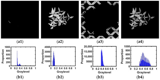
Figure 9.
Extraction effect and corresponding histograms of the soybean canopy under normal treatment: (a1) GRE target image, (a2) NIR target image, (a3) RED target image, (a4) REG target image, (b1) GRE histogram, (b2) NIR histogram, (b3) RED histogram and (b4) REG histogram.
Figure 9 showed that the multispectral images of the normally processed canopy were obtained by the iterative method. The average gray values of the green, NIR, red and red-edge channels were 0.3011, 0.1164, 0.3926 and 0.5343, respectively. The corresponding histograms reached the peak values at 0.2510, 0.1098, 0.3765 and 0.4588, respectively, and the target area of the soybean canopy of the NIR channel was completely divided. Since the edge of the target area of the green and red soybean images were fuzzy and similar to the color of the background area of the soybean image, the image of the target area cannot be obtained effectively, and some leaves were missing in the soybean canopy area of the red-edge channel.
When the iterative threshold method was used to extract the drought-treated soybean canopy’s multispectral image, the thresholds of the green, near-infrared, red and red-edge channel soybean multispectral image were 0.2467, 0.0905, 0.4430 and 0.3131, respectively. The multispectral image of the soybean canopy was calculated and obtained. The histograms of the soybean canopy’s multispectral image were analyzed at the same time. The extraction effect and corresponding histograms of the extracted soybean canopy from the original multispectral image are shown in Figure 10.
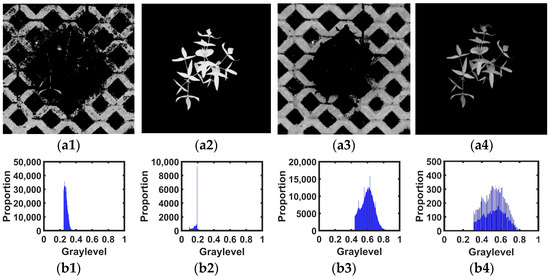
Figure 10.
Extraction effect and corresponding histograms under drought treatment: (a1) GRE target image, (a2) NIR target image, (a3) RED target image, (a4) REG target image, (b1) GRE histogram, (b2) NIR histogram, (b3) RED histogram and (b4) REG histogram.
Figure 10 showed that the average gray values of multispectral images of drought-treated canopy obtained by the iterative method were 0.2760, 0.1688, 0.6022 and 0.5309, respectively, and the corresponding histograms reached the peak values at 0.2549, 0.1922, 0.6314 and 0.5451, respectively. The algorithm can completely segment the soybean canopy target region of the near-infrared channel. After the segmentation of the green and red channels, a large number of background regions were retained, which cannot effectively obtain the image of the target region. Although the soybean canopy area of the red-edge channel was divided, a few background areas were left.
The iterative threshold method had the best segmentation effect for the soybean canopy in the NIR channel. Although most of the target canopy areas can be segmented when segmenting the canopy in the red-edge channel, there will be a lack of some leaves or some background areas. The iterative threshold method was not ideal to extract the soybean canopy in the green channel and the red channel. The size of the soybean green, near infrared, red and red-edge channels was 1280 pixels × 960 pixels. Thus, the NIR image of the soybean canopy was used as the standard template to extract the soybean canopy from the green, red and red-edge channels.
3.2.2. Canopy Extraction from Multispectral Images Based on Standard Template
The NIR reference image of the soybean canopy obtained in Section 3.2.1 was used as the standard template to extract the canopy images from the green channel, red channel and red-edge channel.
The affine transformation was applied to calculate and select the optimal registration parameters of the heterologous images, and an affine transformation model was constructed to extract the soybean canopy from the green, red and red-edge channels, respectively.
- (1)
- Affine transformation principle
Affine transformation was a spatial transformation superimposed by two simple transformations: linear transformation and translation transformation. The spatial changes include spatial position changes such as translation, rotation, scaling, shearing and reflection [30]. For the image with affine transformation, the collinear points still have a collinear relationship before and after transformation, the parallel lines still maintain a parallel relationship and the proportion of variable line segments remains unchanged. Thus, the image also has the characteristics of collinearity, parallelism and collinear proportion invariance after affine transformation [31].
The affine transformation on a two-dimensional Euclidean space can be expressed as:
All geometric transformations can be expressed in the form of the product of a square matrix and a column vector by writing in a homogeneous form. Equation (9) was written in the form of homogeneous coordinates:
where were the coordinates of two corresponding points in the plane; was the translation vector; was the matrix of rotation, scaling and staggered transformation and was a real number.
- (2)
- Registration method
The calibration method based on template matching was used to register the images in the green channel, the red channel and the red-edge channel, respectively, based on the NIR reference image of the soybean canopy. Through the affine transformation algorithm, the NIR reference image was matched with the green channel image, red channel image and red-edge channel image, respectively, and then, the soybean canopy was accurately extracted.
At the same time, the two-dimensional images of the same plant acquired by different sensors could not match completely, which was mainly due to the movement and deformation of image targets caused by the deviation of the sensor angle of view in the imaging process. In order to solve the difficulty of multi-source image matching caused by image deformity, the image gray-based matching method and the image features-based matching method were used to realize a multi-source image fusion. At present, the most widely used matching method is based on image features. When the same target images were acquired by multi-source sensors, the image types and the gray value characteristic were different. The matching method based on image gray was difficult to realize the fusion of the NIR image with green, red and red-edge images. Therefore, the image features-based matching method was adopted for registration. In this study, the canopy edge line and the mapping points between the NIR reference image and the soybean green channel image, the red channel, as well as the red-edge channel image, were used as the feature points and feature lines of multi-source image registration in affine transformation.
- (3)
- Extract the target area
First, the feature points and were calibrated in the image areas of the NIR reference image and the green, red and red-edge channel images, respectively, and then, the corresponding point pairs and in the NIR reference image and canopy target images in the green, red and red-edge channels were searched. Finally, the matching model was established through the corresponding feature points to realize the registration of multi-source images. In the process of image registration, linear geometric transformation was adopted, and the analysis of successive distortion results of the image to be registered was used as the basis for reference image registration. According to the geometric distortion between the NIR reference image of the soybean canopy and the target images in the green, red and red-edge channels, the best-fitting geometric transformation model was selected between the two images, namely the affine transformation model. In this paper, the most commonly used affine transformation model was used to map the points in the reference image to the image to be registered. The mathematical expression was as follows:
where was the translation distance.
The NIR image of the soybean canopy was taken as the reference image, and the affine transformation model for registering the green channel image was as follows:
where was the NIR channel image of the soybean canopy, was the green channel image of the soybean canopy and was the translation distance.
The affine transformation model for registering the red channel image of the soybean canopy was:
where was the NIR channel image of the soybean canopy, was the red channel image of the soybean canopy and was the translation distance.
The affine transformation model for registering the red-edge channel image of the soybean canopy was:
where was the NIR channel image of the soybean canopy, was the red-edge channel image of the soybean canopy and was the translation distance.
After the template coordinate transformation, the target image recognition of the green, red and red-edge channel images was divided into the following three processes.
- (a)
- Read the values of element in row and column of the segmented NIR reference image and the element in row and column of the green, red and red-edge channel image matrix in turn.
- (b)
- Judged whether the value of was 0. If was 0, the value of was also 0. If the value of was not 0, the value of remained unchanged.
- (c)
- Output matrix , which was denoted as the segmentation of the canopy area and background area in the green, red and red-edge channel images of the soybean canopy. Finally, the soybean canopy area was obtained from the green channel, red channel and red-edge channel images, respectively.
When using affine transformation to segment the normally processed multispectral image of the soybean canopy, the NIR canopy image was taken as the standard template, and the green, red and red-edge multispectral image of the soybean canopy was calculated and obtained, and the histogram of the soybean canopy’ multispectral image was analyzed. The registration effect and corresponding histograms of the soybean canopy’s multispectral image are shown in Figure 11.
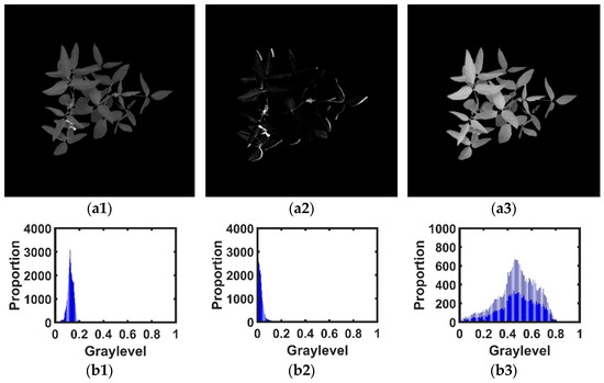
Figure 11.
Extraction effect and corresponding histograms of the soybean canopy under normal treatment: (a1) GRE target image, (a2) RED target image, (a3) REG target image, (b1) GRE histogram, (b2) RED histogram and (b3) REG histogram.
Figure 11 showed that the multispectral image of the normal processing canopy was obtained by affine transformation. The average gray values of the green, NIR, red and red-edge channel were 0.1282, 0.0369 and 0.4544, respectively. Each histogram reached the peak at 0.1255, 0.0118 and 0.4667, respectively, and the soybean canopy target area of the green and red-edge channel was completely divided. Since the color of the soybean canopy in the red channel was too close to the background area, and only most of the target canopy areas was segmented.
When using affine transformation to extract the drought-treated multispectral image of the soybean canopy, the NIR image of the drought-treated soybean canopy was taken as the standard template; the green, red and red-edge multispectral images of the soybean canopy were calculated and obtained and the histogram of the soybean canopy in the multispectral image was analyzed. The extraction effect and corresponding histograms of the soybean canopy’s multispectral image are shown in Figure 12.
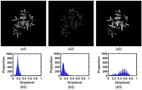
Figure 12.
Extraction effect and corresponding histograms of the soybean canopy under drought treatment: (a1) GRE target image, (a2) RED target image, (a3) REG target image, (b1) GRE histogram, (b2) RED histogram and (b3) REG histogram.
Figure 12 showed that the average gray values of the multispectral images of drought-treated canopy obtained by affine transformation were 0.1766, 0.1227 and 0.4763, respectively, and each histogram reached its peak at 0.1765, 0.0667 and 0.5451, respectively. The soybean canopy target areas of the green, red and red-edge channel were completely divided.
3.2.3. Evaluation of Extraction Effect for Soybean Canopy
Based on the ratio of the pixel number, there were three evaluation indexes: effective segmentation, under segmentation and over segmentation. Effective segmentation can directly reflect the number of correctly segmented pixels in the segmentation results. The lower the over segmentation rate and under segmentation rate, the higher the effective segmentation rate, and the better the segmentation quality.
The effective segmentation rate was defined as:
where was the number of pixels wrongly detected, and was the total number of pixels of the canopy in the standard image.
The smaller the over segmentation rate and under segmentation rate, the better the segmentation performance of the algorithm [32]. The calculation equation was:
where represented the number of pixels that should not be included in the segmentation result but were actually included in the segmentation result, and represented the number of canopy pixels of the standard image. indicated the number of pixels that should be included in the segmentation result but were not.
In the segmentation results of the soybean multispectral image, the effective segmentation rate, over segmentation rate, under segmentation rate and algorithm segmentation time of the soybean canopy’s multispectral image were calculated according to Equations (15)–(17), and the four multispectral images of the soybean canopy in the green, near-infrared, red and red-edge channels were statistically analyzed. The results were shown in Table 3.
Table 3.
Evaluation index results of image segmentation.
Table 3 showed that the average effective segmentation rate using the iterative threshold method and the affine transformation for the extraction of the soybean canopy was more than 95%, and the recognition effect was great. Both algorithms effectively distinguished the canopy and background in the four spectral band images. The average effective segmentation rate was 97.02%, the average under segmentation rate was 2.64% and the average over segmentation rate was 1.83%. The iterative threshold method had the highest effective segmentation rate of 98.17% and the lowest under segmentation rate of 1.06% for the NIR channel. The effective segmentation rate of the canopy extraction algorithm based on affine transformation for the green channel, red channel and red-edge channel was more than 95%. Among them, the under segmentation rate was the highest at 4.29%, because the color of the canopy of some red reflection image was close to that of the background area. In terms of the computing speed, the average processing time of the iterative threshold method and canopy extraction algorithm based on affine transformation were 0.8703 s and 0.7301 s, respectively. Based on the extraction effect of the soybean canopy image, the extraction effect of the two algorithms on the soybean canopy reached an ideal state.
3.3. Calculation Method of Wilting Index for Soybean Canopy Based on Fourier Transform
The Fourier-transform method can transform the image signal information from the time domain to the frequency domain, and the information difficult to observe in the time domain was easy to be observed after being converted to the frequency domain. Thus, Fourier transform was carried out to transform the time domain information of soybean canopy’s multispectral image to a frequency domain for the analysis and calculation of the wilting index for the soybean canopy.
3.3.1. Fourier Transform Principle
Fourier transform was divided into continuous Fourier transform and discrete Fourier transform [33]. In image processing, because the computer saves two-dimensional digital images, this paper used two-dimensional discrete Fourier transform to process multispectral images. The multispectral image was transformed from the time domain to the frequency domain and decomposed into low-frequency components and high-frequency components of different frequencies, and then, the composition structure analysis of each frequency component was realized. The two-dimensional Fourier-transform frequency component distribution diagram is shown in Figure 13.
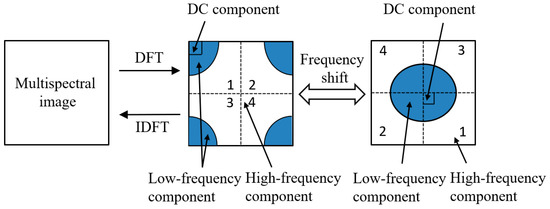
Figure 13.
Two-dimensional Fourier-transform frequency component distribution diagram.
Figure 13 showed that, after the two-dimensional Fourier transform of the multispectral image, the low frequency that included the DC component and high-frequency component was decomposed. After the frequency shift, the low-frequency component was moved from the four corners to the center of the image, and then, the frequency domain was converted to the spatial domain after the inverse Fourier transform.
For any image with size , if the data was two-dimensional discrete, the image must have discrete Fourier transform, which was expressed by Equation (18):
where were the frequency component, were the spatial component, was a natural number, was an imaginary number, was the image and was the frequency spectrum of .
When was given, the corresponding inverse transformation was as follows:
where were the frequency component, were the spatial component, was a natural number, was an imaginary number, was a image and was The frequency spectrum of .
3.3.2. Fourier Transform of the Soybean Canopy’s Multispectral Image
Fourier transform referred to the transformation of the soybean canopy’s multispectral image from time domain space to frequency domain space so as to process and analyze it by using the characteristics of the Fourier spectrum. The calculation efficiency of traditional discrete Fourier transform was low; thus, fast Fourier transform (FFT) was used. At present, there are many fast Fourier transform algorithms. The main algorithms are: the Radix-2 FFT algorithm (time extraction algorithm and frequency domain extraction algorithm), FFT algorithm with a composite number, Split-Radix FFT algorithm, Prime Factor FFT algorithm, Winograd FFT algorithm, multi-dimensional FFT algorithm, FFT algorithm of a real number sequence, Chirp-Z transform algorithm and Zoom-FFT algorithm, but it is basically divided into two categories: decimation-in-time FFT (DIT-FFT) and decimation-in-frequency FFT (DIF-FFT). In this paper, the radix-2 decimation-in-time FFT algorithm was used to carry out Fourier transform for the soybean canopy’s multispectral image.
The radix-2 decimation-in-time FFT algorithm divided the input sequence with length (integer power of two) into two sequences: one contained only the number at the even position in the original sequence: . The other contained only the number at the odd position in the original sequence: , and the length of and was .
The value of the first points of the decomposition sequence was:
The value of the last points of the decomposition sequence was:
Since each decomposition extracted the sequence into two, according to parity in the time domain, it was called the radix-2 decimation-in-time FFT algorithm. After multiple decompositions, it was finally decomposed into the DFT operation combination position of 2 points, and the total amount of multiplication and addition was .
The DFT of the signal with the original length was calculated by Equations (20) and (21). Thus, the DFT of the sequence with the length can be weighted by adding the DFT results of two sequences with the length , which can greatly reduce the amount of calculation.
The process of realizing the Fourier transform of the soybean canopy’s multispectral image by programming was as follows: First, the radix-2 decimation-in-time FFT algorithm was adopted, and the size of the image was required to be a multiple of 2, so the size of the soybean canopy multispectral image matrix used in this study was 128 pixels 128 pixels. Then, the order of each row of the image matrix was reversed and performed by using the butterfly operation. Finally, the order of each column of the matrix obtained in the previous step was reversed and performed by using the butterfly operation to get the result of the Fourier transform of the soybean canopy’s multispectral image.
3.3.3. Spectral Feature Analysis of the Soybean Canopy’s Multispectral Image
The amplitude spectrum, phase spectrum and energy spectrum could be obtained after Fourier transform of the soybean canopy’s multispectral reflection image. The calculation equation of the amplitude spectrum was:
The calculation equation of the phase spectrum was:
The calculation equation of the energy spectrum was:
where and represented the real part and imaginary part of , respectively, and represented the frequency spectrum of the image .
- (1)
- Analysis of the amplitude spectrum and phase spectrum of the soybean canopy’s multispectral image.
The spectral features of the soybean canopy’s multispectral image after Fourier transform were distributed in the four corners of the image. In order to analyze the image more conveniently, the origins of the amplitude spectrum and phase spectrum were shifted to the middle of the image, according to Equation (25), by using the translation characteristics and exponential properties of Fourier transform. In the frequency-shifted amplitude spectrum, the center point was called the DC component, which reflected the average brightness of the original image. Different points at the same distance from the center point had the same frequency and different directions. The closer to the center point, the lower the frequency. The farther away from the center point, the higher the frequency.
where represented the Fourier transform, represented the image with the size of and represented the translation of the origin of the frequency spectrum from to the center point in the frequency coordinates.
The four channels of the soybean canopy’s multispectral image were analyzed by Fourier transform, according to Equation (18), and the Fourier-transform amplitude spectrum and phase spectrum were obtained. According to Equation (25), the spectrum was shifted to the origin point of the image to obtain the amplitude spectrum and phase spectrum after the frequency shift (Figure 14).
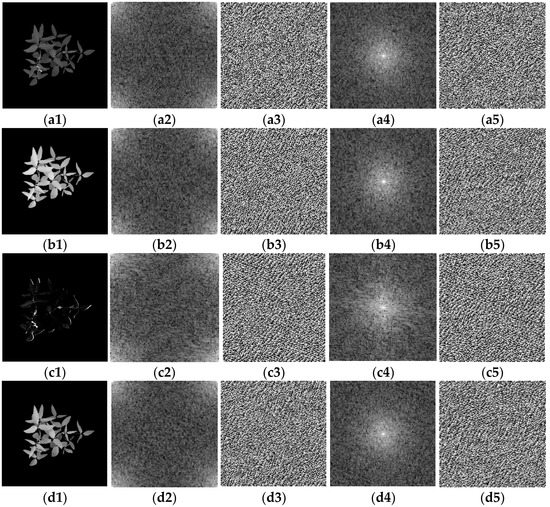
Figure 14.
Amplitude spectrum and phase spectrum of the soybean canopy’s multispectral image: (a1) GRE canopy, (a2) GRE amplitude spectrum, (a3) GRE phase spectrum, (a4) GRE amplitude spectrum after the frequency shift, (a5) GRE phase spectrum after the frequency shift, (b1) NIR canopy, (b2) NIR amplitude spectrum, (b3) NIR phase spectrum, (b4) NIR amplitude spectrum after the frequency shift, (b5) NIR phase spectrum after the frequency shift, (c1) RED canopy, (c2) RED amplitude spectrum, (c3) RED phase spectrum, (c4) RED amplitude spectrum after the frequency shift, (c5) RED phase spectrum after the frequency shift, (d1) REG canopy, (d2) REG amplitude spectrum, (d3) REG phase spectrum, (d4) REG amplitude spectrum after the frequency shift and (d5) REG phase spectrum the after frequency shift.
Figure 14a2,b2,c2,d2,a4,b4,c4,d4 amplitude spectra showed that the low-frequency components after frequency shift were concentrated around the center of the amplitude spectrum from four angles. The reflection images of the green, near-infrared, red and red-edge channels of the soybean canopy contained the sum of each frequency component of 5,646,242, 5,012,815, 3,771,802 and 22,279,084, respectively. At the same time, the intensity distribution of each frequency amplitude showed the frequency distribution of soybean multispectral images after Fourier transform, which can reflect the ecological and morphological characteristics of soybeans. It can be seen from the phase spectra (a3–d3) and (a5–d5) in Figure 14 that they only contained some random signals and could not directly obtain useful information. Therefore, in this paper, the amplitude spectrum was only used to analyze the soybean canopy wilting index during multispectral image processing.
- (2)
- Energy spectrum analysis of the soybean canopy’s multispectral image.
In order to observe the distribution of each spectral component in the amplitude spectrum more clearly and further calculate the energy information of the spectral component, the energy spectrum of the soybean canopy’s multispectral image after Fourier transform was analyzed below.
According to Equation (24), the energy spectrum was defined as the square of the amplitude spectrum. The energy spectrum represented the energy characteristics of the image and described the distribution of the signal energy in each frequency range. Generally, the frequency band of the image signal was limited, and the energy spectrum of the image decreased rapidly with the increase of the frequency, resulting in a great difference between the energy of the low-frequency part and high-frequency part. In order to clearly display the low-frequency energy and high-frequency energy at the same time, the Fourier-transform energy spectrum was coordinate-shifted and logarithmically processed. The reflection images of the soybean canopy were conducted by Fourier transform under normal treatment and drought treatment, respectively, and the zero-order spectral coefficient at the center of the two-dimensional spectral coefficient matrix was placed to obtain the energy spectrum reflecting the spectral energy information (Figure 15).
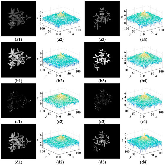
Figure 15.
Energy spectrum of the soybean canopy’s multispectral image: (a1) GRE canopy under normal treatment, (a2) GRE energy spectrum under normal treatment, (a3) GRE canopy under drought treatment, (a4) GRE energy spectrum under drought treatment, (b1) NIR canopy under normal treatment, (b2) NIR energy spectrum under normal treatment, (b3) NIR canopy under drought treatment, (b4) NIR energy spectrum under drought treatment, (c1) RED canopy under normal treatment, (c2) RED energy spectrum under normal treatment, (c3) RED canopy under drought treatment, (c4) RED energy spectrum under drought treatment, (d1) REG canopy under normal treatment, (d2) REG energy spectrum under normal treatment, (d3) REG canopy under drought treatment and (d4) REG energy spectrum under drought treatment.
Figure 15a2,b2,c2,d2,a4,b4,c4,d4 showed a series of areas with different colors on the energy spectrum. These different colors indicated the spectral energy distribution of the soybean canopy’s multispectral image. Where the spectral energy was large, the color of the point was yellow; on the contrary, it tended toward green. Thus, most of the spectral energy of the soybean canopy’s multispectral image was concentrated near the low-frequency component of the energy spectrum. The energy diffused from the center to the periphery, and the energy of the high-frequency component was relatively weak, which was distributed on the edge of the energy spectrum. According to Equations (26)–(28), the spectral energy of the soybean canopy’s multispectral image was calculated under normal treatment and drought treatment, respectively, and the distribution and characteristics of the spectral energy of the energy spectrum were analyzed under normal treatment (Figure 15a2,b2,c2,d2) and drought treatment (Figure 15a4,b4,c4,d4), respectively.
On the energy spectrum, a series of concentric rings were made with the spectrum center as the center and R as the radius. The distribution of the corresponding spectrum energy was characterized by the percentage of the spectrum energy contained in circles with different radius sizes in the total spectrum energy [34]. The calculation equation was as follows:
where represented the frequency component, represented the image size, represented the spectrum and represented the energy spectrum.
According to Equations (26)–(28), the spectrum energy was analyzed and calculated under normal treatment and drought treatment in the green channel under a different spectrum radius (Table 4).
Table 4.
Spectrum energy distribution of the soybean canopy in the green channel.
Table 4 showed that, when the spectrum radius was 15, the energy in the green channel under normal treatment reached 90.47% of the total spectrum energy. When the radius was 50, the energy reached 99.82%, while the energy under drought treatment only reached 78.04% of the total spectrum energy when the spectrum radius was 15, and the energy reached 99.52% when the radius was 50. Thus, for the energy spectrum of the green channel in Figure 15a2,a4, when the spectrum radius was 15, 25, 35 and 50, the spectral energy of the soybean canopy under drought treatment was less than that under normal treatment.
Similarly, according to Equations (26)–(28), the spectrum energy was analyzed and calculated under normal treatment and drought treatment in the NIR channel under different spectrum radii (Table 5).
Table 5.
Spectrum energy distribution of the soybean canopy in the NIR channel.
Table 5 showed that, when the spectrum radius was 15, the energy under normal treatment in the NIR channel reached 91.18% of the total spectrum energy. When the radius was 50, the energy reached 99.84%, while, when the spectrum radius was 15, the energy under drought treatment only reached 82.73% of the total spectrum energy. When the radius was 50, the energy reached 99.72%. Therefore, for the energy spectra of the NIR channels in Figure 15b2,b4, the spectral energy of the soybean canopy under drought treatment was less than that under normal treatment when the spectral radius was 15, 25, 35 and 50, respectively.
Similarly, according to Equations (26)–(28), the spectrum energy under normal treatment and drought treatment under different spectrum radii in the red channel was analyzed and calculated (Table 6).
Table 6.
Spectrum energy distribution of the soybean canopy in the red channel.
Table 6 showed that, when the spectrum radius was 15, the energy under normal treatment in the red channel reached 58.33% of the total spectrum energy. When the spectrum radius was 50, the energy reached 98.44%. The energy under drought treatment reached 67.55% of the total spectrum energy when the spectrum radius was 15. The energy reached 98.98% when the spectrum radius was 50, because the color of the soybean canopy under normal treatment in the red channel was similar to the background area, resulting in a poor extraction effect. For the energy spectrum in the red channel in Figure 15c2,c4, the spectral energy under drought treatment was greater than that under normal treatment when the spectral radius was 15, 25, 35 and 50, respectively.
Similarly, according to Equations (26)–(28), the spectrum energy under normal treatment and drought treatment in the red-edge channel was analyzed and calculated under different spectrum radii (Table 7).
Table 7.
Spectrum energy distribution of the soybean canopy in the red-edge channel.
Table 7 showed that, when the spectrum radius was 15, the energy of the soybean canopy under normal treatment in the red-edge channel reached 90.90% of the total spectrum energy. When the radius was 50, the energy reached 99.85%, while, when the spectrum radius was 15, the energy under drought treatment only reached 81.89% of the total spectrum energy. When the radius was 50, the energy reached 99.73%. Thus, for the energy spectrum of the red-edge channel in Figure 15d2,d4, the spectral energy under drought treatment was less than that under normal treatment when the spectral radius was 15, 25, 35 and 50, respectively.
By analyzing the spectral characteristics of the soybean canopy’s multispectral images on the energy spectra of normal treatment and drought treatment, most of the spectral energy was concentrated in the low-frequency region of the spectrum center—that was, most of the energy after Fourier transform was concentrated in the low-order spectrum coefficient. At the spectral radius of 15, 25, 35 and 50, except for the influence of the red channel on the canopy extraction effect, the percentage of spectral energy of the soybean canopy’s multispectral images under drought treatment in the green, near-infrared and red-edge channels in the total energy was less than that under normal treatment. Therefore, according to this spectral characteristic, the wilting index was calculated based on the energy spectrum of Fourier transform.
3.3.4. Formulation of Wilting Index for the Soybean Canopy
The mathematical significance of the Fourier spectrum method was that, if the morphology of the soybean leaves changed from stretching to wilting, it indicated that the slope of each point of the leaf surface changed in varying degrees. From the Fourier spectrum, the low-frequency spectrum decreased, and the high-frequency spectrum increased. Thus, the wilting index for the soybean canopy can be obtained by spectral decomposition.
For a plane image, most frequencies correspond to very small amplitudes after Fourier transform, but the amplitude at the frequency zero suddenly appeared as the highest point—that was, the amplitude of the DC component was the largest. This point value represented the number of points with a frequency of zero. When the soybean canopy did not wilt, the leaf surface could be approximately regarded as a plane. At this time, the points with a frequency of zero were the most, and the DC component of the Fourier spectrum was the largest. When the leaf wilted, the curvature of the leaf increased, the point with zero decreased and the value of the DC component decreased. Therefore, the DC component after Fourier transform could be used to investigate the wilting degree of the soybean canopy.
The data on the soybean canopy surface was aperiodic discrete signal. The spectrum information was obtained by Fourier transform. The DC component in the spectrum represented the plane component of the surface, and the high-order harmonic component represented the surface components with different bending degrees on the surface. The proportion of the DC component in the spectrum can quantitatively represent the wilting degree of the plant leaves. Based on this, the soybean wilting index based on the Fourier-transform energy spectrum was defined as:
where represented the amplitude of the DC component in the energy spectrum, and represented the total amplitude of the spectrum in the energy spectrum.
4. Results and Analysis
4.1. Analysis of Wilting Index for Soybean Canopy
The steps of calculating the wilting index of the soybean canopy’s multispectral image were as follows: First, the soybean canopy’s multispectral image was extracted by the iterative threshold method and canopy extraction algorithm based on affine transformation. Then, the extracted soybean canopy was transformed into a binary image by the adaptive binarization method. Finally, the spectrum was obtained by Fourier transform, the DC component was extracted from the spectrum information and the wilting index of the soybean canopy was calculated according to Equation (29).
According to the above process of calculating the wilting index, a Fourier transform analysis was carried out on the four-channel multispectral images of the soybean canopy under normal treatment and drought treatment in the V4 stage. The soybean canopy and its corresponding spectrum are shown in Figure 16.
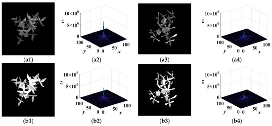
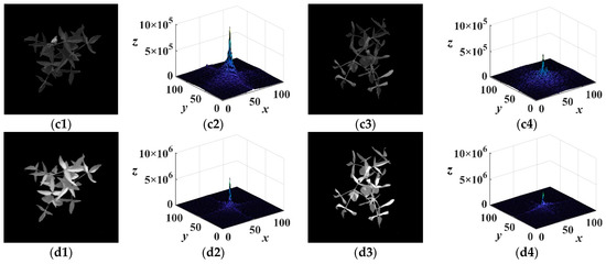
Figure 16.
Soybean canopy and corresponding spectrum: (a1) GRE canopy under normal treatment, (a2) GRE spectrum under normal treatment, (a3) GRE canopy under drought treatment, (a4) GRE spectrum under drought treatment, (b1) NIR canopy under normal treatment, (b2) NIR spectrum under normal treatment, (b3) NIR canopy under drought treatment, (b4) NIR spectrum under drought treatment, (c1) RED canopy under normal treatment, (c2) RED spectrum under normal treatment, (c3) RED canopy under drought treatment, (c4) RED spectrum under drought treatment, (d1) REG canopy under normal treatment, (d2) REG spectrum under normal treatment, (d3) REG canopy under drought treatment and (d4) REG spectrum under drought treatment.
At the same time, the DC component of the spectrum of the four channels was calculated for the soybean canopy’s multispectral image in Figure 16, and the wilting index of the four channels of the soybean canopy was calculated according to Equation (29) (Table 8).
Table 8.
Wilting index of the soybean canopy multispectral image in the V4 stage.
Table 8 showed that the soybean canopy wilted seriously after the drought treatment in V4. Fourier transform was performed on the canopy images of the soybean green, near-infrared, red and red-edge channels, respectively. The DC component of the images of each channel was lower than that of the normal treatment; the sum of each harmonic was smaller and the wilting index increment was 5.50, 6.30, 7.63 and 5.84, respectively. Therefore, the wilting index of the spectral images of each channel in the V4 period can reflect the physiological and ecological characteristics of the soybean canopy.
Similarly, a Fourier-transform analysis was carried out on the four channels of the multispectral images for the soybean canopy under normal treatment and drought treatment in the V5 stage. The soybean canopy and its corresponding spectrum are shown in Figure 17.
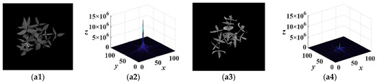
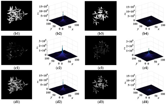
Figure 17.
Soybean canopy and the corresponding spectrum: (a1) GRE canopy under normal treatment, (a2) GRE spectrum under normal treatment, (a3) GRE canopy under drought treatment, (a4) GRE spectrum under drought treatment, (b1) NIR canopy under normal treatment, (b2) NIR spectrum under normal treatment, (b3) NIR canopy under drought treatment, (b4) NIR spectrum under drought treatment, (c1) RED canopy under normal treatment, (c2) RED spectrum under normal treatment, (c3) RED canopy under drought treatment, (c4) RED spectrum under drought treatment, (d1) REG canopy under normal treatment, (d2) REG spectrum under normal treatment, (d3) REG canopy under drought treatment and (d4) REG spectrum under drought treatment.
At the same time, the DC component of the four channels’ spectrum for the soybean’s multispectral image in Figure 17 was extracted, and the wilting index of the four channels’ spectrum of the soybean in Figure 17 was calculated according to Equation (29) (Table 9).
Table 9.
Wilting index of the soybean canopy’s multispectral image in the V5 stage.
Table 9 showed that, due to the serious wilting of the soybean canopy under drought treatment in V5, after the spectral canopy of the green, near-infrared, red and red-edge channels in the soybean multispectral images was Fourier-transformed, compared with the normal treatment, the DC component value was lower; the sum of each harmonic was smaller and the wilting index increased by 11.24, 11.30, 2.30 and 12.39, respectively. Since the color of the soybean canopy under the normal treatment of the red channel was too close to the background area and part of the canopy area was missing after binarization, resulting in a low DC component value and high wilting index after Fourier transform, the wilting index of the soybeans under the condition of the drought treatment was slightly different from that under the normal treatment. Therefore, the canopy wilting index calculated by each channel of the soybeans in the V5 period also reflected the physiological and ecological characteristics of the soybean.
The wilting indexes in the four channels of Fourier transform for the soybean canopy’s multispectral images under the normal and drought treatments in V4 and V5 were statistically analyzed, with a total of 60 groups. The analysis result was as shown in Figure 18.

Figure 18.
Wilting index of multispectral images of the soybean canopy under normal treatment and drought treatment: (a) wilting index in the GRE channel, (b) wilting index in the NIR channel, (c) wilting index in the RED channel and (d) wilting index in the REG channel.
In Figure 18, C represented the normal treatment, and D represented the drought treatment. The wilting indexes of the four channels for the soybean canopy’s multispectral images in V4 and V5 were statistically analyzed, and the results are shown in Table 10.
Table 10.
Statistical analysis of the soybean canopy wilting index.
Table 10 showed that drought treatment caused the soybean to be subjected to water stress, and the soybean canopy wilted. The average wilting index in the four channels was higher than that under the normal treatment. The difference between the average wilting index under the normal treatment in the green, NIR, red and red-edge and the average wilting index of the drought treatment was 2.38, 3.11, 3.56 and 4.11. Therefore, through the calculation of the wilting index of the four channels of the soybean canopy’s multispectral image, the red-edge channel was the best to distinguish between normal treatment and drought treatment, while the green channel was the poorest.
4.2. Validation Analysis of Calculation Method for Wilting Index
Leaf inclination referred to the angle between the normal leaf ventral surface and the main stem, as well as the angle between the leaf surface and the ground plane [35]. A large number of studies showed that the leaf inclination of the plant had a significant correlation with the soil–water content [36,37,38,39]. Therefore, we can verify the effectiveness of the soybean wilting index in reflecting the water deficit of soybeans by analyzing the correlation between the change of the soybean leaf inclination and the wilting index. In this paper, the correlation analysis between the wilting index in the four channels and the average leaf inclination in the corresponding stage was carried out under normal treatment and drought treatment in the V4 and V5 growth stages to verify the effectiveness of the wilting index calculation method. The results are shown in Table 11.
Table 11.
Correlation analysis between the soybean wilting index and average leaf inclination.
Table 11 showed that the determination coefficient R2 of the measured values of the wilting index and leaf inclination of the soybean canopy in V4 and V5 were distributed between 0.85~0.94 and 0.85~0.95, with average values of 0.90 and 0.89, respectively. In V4, the maximum value of R2 for the normal water supply and drought treatment was 0.94 for the red-edge channel and 0.92 for the NIR channel, respectively, and the minimum value was 0.88 and 0.85 for the green and red channels, respectively. The wilting index of the two treatments in V5 showed certain changes. The maximum value of R2 was 0.87 and 0.95 for the red-edge and red channels, respectively, and the minimum value was 0.85 for the NIR channel and 0.88 for the green channel, respectively. The results showed that the wilting index defined in this paper had a strong correlation with the leaf inclination, which could be used to calculate the wilting degree of the soybean and reflect the water shortage of the soybean.
5. Discussion
In this paper, through the extraction of the soybean canopy from the multispectral image and Fourier transform for the extracted soybean canopy, the characteristics of the energy spectrum were analyzed, and the soybean wilting index was proposed based on the energy spectrum of Fourier transform, which can be used to describe the wilting degree of soybean plants.
- (1)
- Advantage analysis of the proposed method
In this paper, a method for calculating wilting index of a soybean canopy was proposed by processing multispectral images (green, NIR, red and red-edge channels). The determination coefficient R2 of the canopy wilting index and leaf inclination angle of the soybean canopy reached more than 0.85, which could provide a quantitative basis for the scientific evaluation and regulation of the ecological and morphological characteristics of soybean plants under drought stress. This method avoids the following situations: First, the single-band spectrum was easily affected by interference factors, such as light intensity and weather factors. Second, the plant physiological and ecological information does not change significantly in a certain single spectrum, resulting in inaccurate detection results or even errors. Thus, the proposed method of this paper detected the crop canopy wilt degree based on multiple band spectra, which can more comprehensively reflect the comprehensive situation of the plant growth status, avoiding or reducing the detection error of a single spectrum to the greatest extent, and improved the reliability and anti-interference ability of the wilting degree’s detection method for the soybean canopy.
The proposed method here organically fused the time–frequency characteristics of the soybean canopy’s multispectral images, analyzed the heterogeneity in the frequency domain and the dynamics in the time domain of the soybean canopy under drought stress, characterized the ecological and morphological characteristics of soybean organs and nondestructively measured the wilting index of the soybean canopy. At present, the calculation of the crop plant wilting mostly focuses on the spatial morphological expression of the canopy. References [19,20,21,22,23] used the acquisition technology of the laser point cloud and RGB image processing methods to characterize the wilting degree through the morphological changes of the plant canopy. Both visible light image analysis technology and three-dimensional structure change of the point cloud were based on the apparent change of the physical structures of the plant canopy organs. When plants were stressed by water, nutrition and diseases, the internal structure changes of the organs, tissues and cells preceded the morphological changes. Thus, in this paper, the images formed by multi-band spectral reflectance values were used to reflect the early changes in the soybean canopy organs under drought stress—that is, before the visible light and three-dimensional morphological changes were observed by the naked eye, the physiological and ecological character information of each organ in the canopy can be detected, and the calculation method of the quantitative index for the early canopy’s phenotypic characteristics of soybeans under drought stress can be realized.
- (2)
- Experimental error analysis
The calculation of the wilting index was aimed at the soybean canopy. Therefore, the canopy extraction from the soybean canopy’s multispectral image was a crucial step. The effect of canopy extraction directly affected the calculation results of the wilt index. In addition, when collecting the experimental data, the light also had an impact on the imaging of the Sequoia multispectral camera, especially on the red channel image. The multispectral image of the soybean canopy first obtained on the day of collecting the data in this study was dark due to the low-light intensity. When extracting the canopy from the red channel, the canopy color was similar to the color of the background area, resulting in a poor extraction effect. With the progress of the experiment, the light intensity became stronger, and the imaging effect of the acquired multispectral images was better. Through the extraction algorithm based on affine transformation, the soybean canopy in the red channel could be extracted completely. If these two problems were solved, the calculation effect of the soybean wilting index would be improved further.
- (3)
- Future promotion and application
The calculation method of the wilting index based on the energy spectrum of Fourier transform proposed in this paper is not only suitable for the calculation of the soybean wilting degree but can also be extended to all kinds of crops. It is not limited to crops under drought stress but can also be used to calculate crop canopy wilting caused by crop nitrogen deficiency or salt alkali stress. Through the acquisition of a crop’s multispectral imaging information, the nondestructive and rapid detection of crops’ physiological and ecological information have been widely used in the field of intelligent agriculture. In particular, Near-Earth multispectral technology has the advantages of low instrument cost, convenient detection and high image resolution, which had attracted more and more attention of agricultural scientists. Thus, the proposed method of the wilting index can provide a new idea for the evaluation of a crop’s wilting degree.
6. Conclusions
In this paper, the acquisition system was constructed to obtain the soybean canopy’s multispectral image in V4 and V5. The original multispectral image was transformed into a reflection image by using the empirical linear method. The soybean canopy was extracted by using the iterative threshold method and affine transform. After the soybean canopy was Fourier-transformed, the spectral characteristics of the soybean canopy’s multispectral image were analyzed, and the soybean wilting index, based on the energy spectrum of Fourier transform, was proposed. The effectiveness of the calculation method of the wilting index was verified by a correlation analysis with the average leaf inclination.
- (1)
- Multispectral image extraction of the soybean canopy
For the energy spectra under normal treatment and drought treatment, most of the spectrum energy was concentrated in the low-frequency region of the spectrum center. When the spectrum radius was 15, 25, 35 and 50, except that the red channel was affected by the canopy extraction effect, the percentage of the spectrum energy of the multispectral images of the soybean canopy under drought treatment in the total energy was less than that of the normal treatment, and the energy of each channel reached more than 98% when the spectrum radius was 50.
- (2)
- Energy spectrum characteristics of the soybean canopy
For the energy spectra under normal treatment and drought treatment, most of the spectrum energy was concentrated in the low-frequency region of the spectrum center. When the spectrum radius was 15, 25 and 35, except for the red channel, the percentage of the spectrum energy of the soybean canopy’s multispectral image under drought treatment in the total energy was less than that under normal treatment, and the energy of each channel reached more than 98% when the spectrum radius was 55.
- (3)
- Wilting index of soybean canopy based on energy spectrum of Fourier transform
The average wilting index under drought treatment in the green, NIR, red and red-edge channel was greater than that under the normal treatment, and the difference of the wilting index was 2.38, 3.11, 3.56 and 4.11, respectively. Among them, the effect of distinguishing the canopy characteristics of the red-edge channel was the best and in the green channel was the worst. The effectiveness of the proposed soybean canopy’s wilting index was verified through a correlation analysis with the average leaf inclination. The wilting index and the determination coefficient R2 of the average leaf inclination in the four channels were more than 0.85, indicating that the proposed soybean canopy’s wilting index can provide a quantitative basis and technical support for the scientific regulation of the soybean plant’s ecology and morphological phenotypes while under drought stress.
Author Contributions
Conceptualization, X.M.; data curation, P.S.; investigation, P.S., H.G., H.H., F.W., M.Y. and C.Y.; methodology, P.S. and X.M.; resources, X.M.; writing—original draft, P.S. and writing—review and editing, X.M. All authors have read and agreed to the published version of the manuscript.
Funding
This study was funded jointly by the National Natural Science Foundation of China (funding code: 31601220), the Natural Science Foundation of Heilongjiang Province, China (funding codes: LH2021C062 and LH2020C080) and the Heilongjiang Bayi Agricultural University Support Program for San Heng San Zong, China (funding codes: TDJH202101 and ZRCQC202006).
Institutional Review Board Statement
Not applicable.
Informed Consent Statement
Not applicable.
Data Availability Statement
All data are presented within the article.
Conflicts of Interest
The authors declare that they have no conflict of interest.
References
- Iftikhar, I.; Anwar-ul-Haq, M.; Akhtar, J. Exogenous Osmolytes Supplementation Improves the Physiological Characteristics, Antioxidant Enzymatic Activity and Lipid Peroxidation Alleviation in Drought-Stressed Soybean. Pak. J. Agric. Sci. 2022, 59, 43–53. [Google Scholar]
- Basal, O.; Szabó, A.; Veres, S. Physiology of Soybean as Affected by PEG-Induced Drought Stress. Curr. Plant Biol. 2020, 22, 100135. [Google Scholar] [CrossRef]
- Wang, X.; Zhang, Y.J.; Li, Y.; Liu, T.; Zhang, J.; Qi, X. Effects of Drought Stress on Soybean Growth and Selection of Drought Resistance Evaluation Methods and Indicators. J. Plant Genet. Resour. 2018, 19, 49–56. [Google Scholar]
- Steketee, C.J.; Schapaugh, W.T.; Carter, T.E., Jr. Genome-Wide Association Analyses Reveal Genomic Regions Controlling Canopy Wilting in Soybean. G3 Genes Genomes Genet. 2020, 10, 1413–1425. [Google Scholar] [CrossRef] [Green Version]
- Ahmed, A.A.M.; Mohamed, E.A.; Hussein, M.Y. Genomic Regions Associated with Leaf Wilting Traits under Drought Stress in Spring Wheat at the Seedling Stage Revealed by GWAS. Environ. Exp. Bot. 2021, 184, 104393. [Google Scholar] [CrossRef]
- Ramos-Giraldo, P.; Reberg-Horton, C.; Locke, A.M. Drought Stress Detection Using Low-Cost Computer Vision Systems and Machine Learning Techniques. IT Prof. 2020, 22, 27–29. [Google Scholar] [CrossRef]
- Sarkar, S.; Ramsey, A.F.; Cazenave, A.B. Peanut Leaf Wilting Estimation from RGB Color Indices and Logistic Models. Front. Plant Sci. 2021, 12, 713. [Google Scholar] [CrossRef]
- Li, D.; Jin, K.; Li, X.; Cao, J.; Han, W.; Liu, Y.; Li, W. Research Progress on Identification and Evaluation Methods of Drought Resistance of Soybean. J. North. Agric. 2020, 48, 48–53. [Google Scholar]
- Li, S.; Cao, Y.; Wang, C.; Wang, W.; Song, S. Research Progress on Physiology and Genetics of Soybean Canopy Wilt Resistance. J. Plant Genet. Resour. 2020, 21, 1321–1328. [Google Scholar]
- Wang, G.; Zhou, Q.; He, M. Wilting Index and Root Morphological Characteristics Used as Drought-Tolerance Variety Selection at the Seedling Stage in Soybean (Glycine max L.). Plant Growth Regul. 2020, 92, 29–42. [Google Scholar] [CrossRef]
- Ma, X.; Zhu, K.; Guan, H. High-Throughput Phenotyping Analysis of Potted Soybean Plants Using Colorized Depth Images Based on a Proximal Platform. Remote Sens. 2019, 11, 1085. [Google Scholar] [CrossRef] [Green Version]
- Zhang, Z.; Ma, X.; Guan, H. A Method for Calculating the Leaf Inclination of Soybean Canopy Based on 3D Point Clouds. Int. J. Remote Sens. 2021, 42, 5721–5742. [Google Scholar] [CrossRef]
- Zhu, K.; Ma, X.; Guan, H.; Feng, J.; Zhang, Z.; Yu, S. A Method of Calculating the Leafstalk Angle of the Soybean Canopy Based on 3D Point Clouds. Int. J. Remote Sens. 2021, 42, 2463–2484. [Google Scholar] [CrossRef]
- Lama, G.F.C.; Crimaldi, M. Remote Sensing of Ecohydrological, Ecohydraulic and Ecohydrodynamic Phenomena in Vegetated Waterways: The Role of Leaf Area Index (LAI). Biol. Life Sci. Forum 2021, 3, 54. [Google Scholar]
- McGlade, J.; Wallace, L.; Reinke, K.; Jones, S. The Potential of Low-Cost 3D Imaging Technologies for Forestry Applications: Setting a Research Agenda for Low-Cost Remote Sensing Inventory Tasks. Forests 2022, 13, 204. [Google Scholar] [CrossRef]
- Guimarães, N.; Pádua, L.; Marques, P.; Silva, N.; Peres, E.; Sousa, J.J. Forestry Remote Sensing from Unmanned Aerial Vehicles: A Review Focusing on the Data, Processing and Potentialities. Remote Sens. 2020, 12, 1046. [Google Scholar] [CrossRef] [Green Version]
- Jalonen, J.; Järvelä, J.; Virtanen, J.P.; Vaaja, M.; Kurkela, M.; Hyyppä, H. Determining Characteristic Vegetation Areas by Terrestrial Laser Scanning for Floodplain Flow Modeling. Water 2015, 7, 420–437. [Google Scholar] [CrossRef] [Green Version]
- Sadeghifar, T.; Lama, G.F.C.; Sihag, P.; Bayram, A.; Kisi, O. Wave Height Predictions in Complex Sea Flows through Soft Computing Models: Case Study of Persian Gulf. Ocean. Eng. 2022, 245, 110467. [Google Scholar] [CrossRef]
- Zhao, Y.; Liu, H.; Liu, W. Measurement Method of Plant Wilting under Water Deficit Stress Based on Leaf Fractal Dimension. J. Agric. Eng. 2011, 27, 191–195. [Google Scholar]
- Zhang, H.; Zhao, Y.; Sun, Y. Identification Method of Plant Wilting State under Water Deficit Stress Based on 3D Image. J. Agric. Mach. 2011, 42, 154–158. [Google Scholar]
- Cai, X.; Sun, Y.; Zhao, Y. Smart Detection of Leaf Wilting by 3D Image Processing and 2D Fourier Transform. Comput. Electron. Agric. 2013, 90, 68–75. [Google Scholar] [CrossRef]
- Zheng, L.; Sun, Y.; Cai, X. Identification of Plant Water Deficit State and Comparison of Wilting Index Based on Laser Scanning 3D Image. J. Agric. Eng. 2015, 31, 79–86. [Google Scholar]
- Zhang, X.; Gao, G.; Martin, K.; Zhao, Y. Identification of Plant Leaf Wilting Based on TOF Camera. J. Agric. Mach. 2016, 47, 275–280. [Google Scholar]
- Peng, Y.; Xiao, Y.; Fu, Z.; Dong, Y.; Li, X.; Yan, H.; Zheng, Y. Detection of Water Content in Maize Leaves Based on Multispectral Images. Spectrosc. Spectr. Anal. 2020, 40, 1257–1262. [Google Scholar]
- Poncet, A.M.; Knappenberger, T.; Brodbeck, C. Multispectral UAS Data Accuracy for Different Radiometric Calibration Methods. Remote Sens. 2019, 11, 1917. [Google Scholar] [CrossRef] [Green Version]
- Mei, L.; Gou, S. Application of a Weighted Median Filter Algorithm in Medical Magnetic Resonance Image Denoising. J. Yanbian Univ. 2021, 47, 365–369. [Google Scholar]
- Li, W.; Chen, J.; Zhang, Y.; Shi, X. Research on Medical Image Denoising Based on Improved Weighted Mean Filtering. J. Liaoning Univ. 2022, 49, 30–35. [Google Scholar]
- Sun, B.; Zhao, Z.; Xie, D. Sparse Spectral Signal Reconstruction for One Proposed Nine-Band Multispectral Imaging System. Mech. Syst. Signal Process. 2020, 141, 106627. [Google Scholar] [CrossRef]
- Li, G.; Wang, T. Research on Concrete Crack Detection Based on Morphological Processing and Feature Analysis. Build. Struct. 2020, 50, 529–533. [Google Scholar]
- Wang, F.; Li, X. Infrared and Visible Image Fusion Based on Two-Level Decision Rules. Semicond. Optoelectron. 2020, 41, 283–286. [Google Scholar]
- Ma, J.; Chen, C.; Li, C. Infrared and Visible Image Fusion via Gradient Transfer and Total Variation Minimization. Inf. Fusion 2016, 31, 100–109. [Google Scholar] [CrossRef]
- Han, Q.; Zhao, Y.; Zhao, Y. Pore Segmentation in Soil Tomography Image Based on Full Convolution Network. J. Agric. Eng. 2019, 35, 128–133. [Google Scholar]
- Sun, T.; Hu, H. Nonlinear dynamics analysis of planetary gear system based on discrete Fourier transform and harmonic balance method. J. Mech. Eng. 2002, 38, 58–61. [Google Scholar] [CrossRef]
- Wu, G.; Xiao, P.; Feng, X.; Wang, K. Using spectral energy to recognize ground objects in high-resolution remote sensing images. J. Wuhan Univ. (Inf. Sci. Ed.) 2011, 36, 1294–1297. [Google Scholar]
- Su, W.; Guo, H.; Zhao, D.; Liu, T.; Zhang, M. Lai Inversion Method of Maize Based on Optimizing PROSAIL Leaf Inclination Distribution Function. J. Agric. Mach. 2016, 47, 234–241. [Google Scholar]
- Fu, K.; Feng, Q.; Yang, S.; Chen, B. Monitoring and Experimental Verification of Strawberry Leaf Moisture Content Using 3D Geometric Features. J. Agric. Eng. 2020, 36, 161–169. [Google Scholar]
- Lazarević, B.; Šatović, Z.; Nimac, A. Application of Phenotyping Methods in Detection of Drought and Salinity Stress in Basil (Ocimum basilicum L.). Front. Plant Sci. 2021, 12, 174. [Google Scholar] [CrossRef]
- An, J.; Li, W.; Li, M. Identification and Classification of Maize Drought Stress Using Deep Convolutional Neural Network. Symmetry 2019, 11, 256. [Google Scholar] [CrossRef] [Green Version]
- Guo, Z.; Gong, D.; Mei, X.; Hao, W.; Li, Y.; Liu, B. Effects of Drought Rehydration on Canopy Structure and Water Use Efficiency of Different Maize Varieties. J. Irrig. Drain. 2011, 30, 41–45. [Google Scholar]

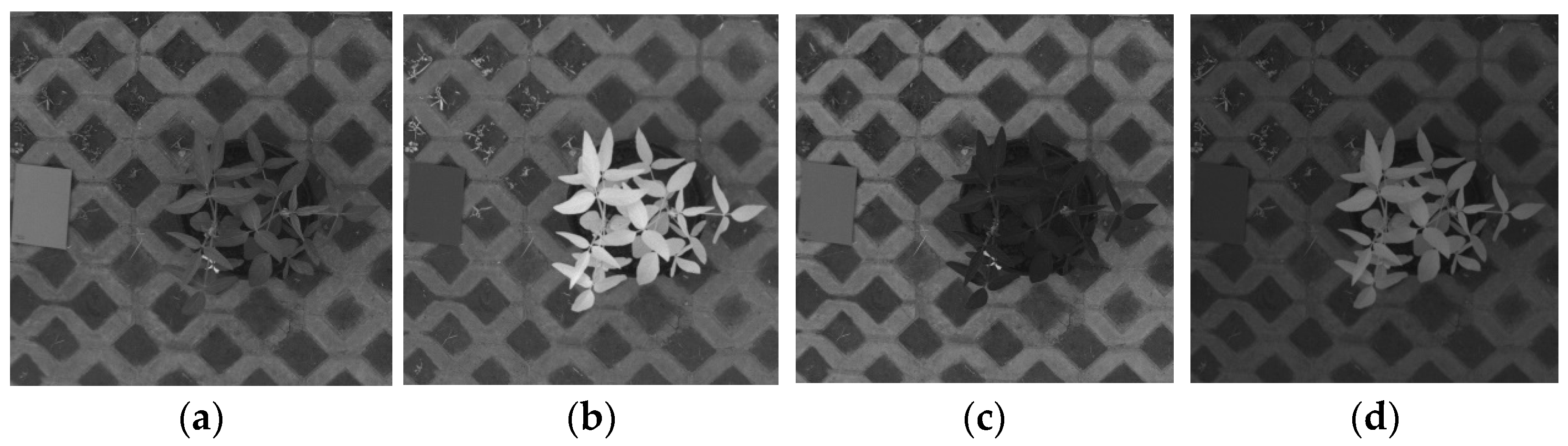
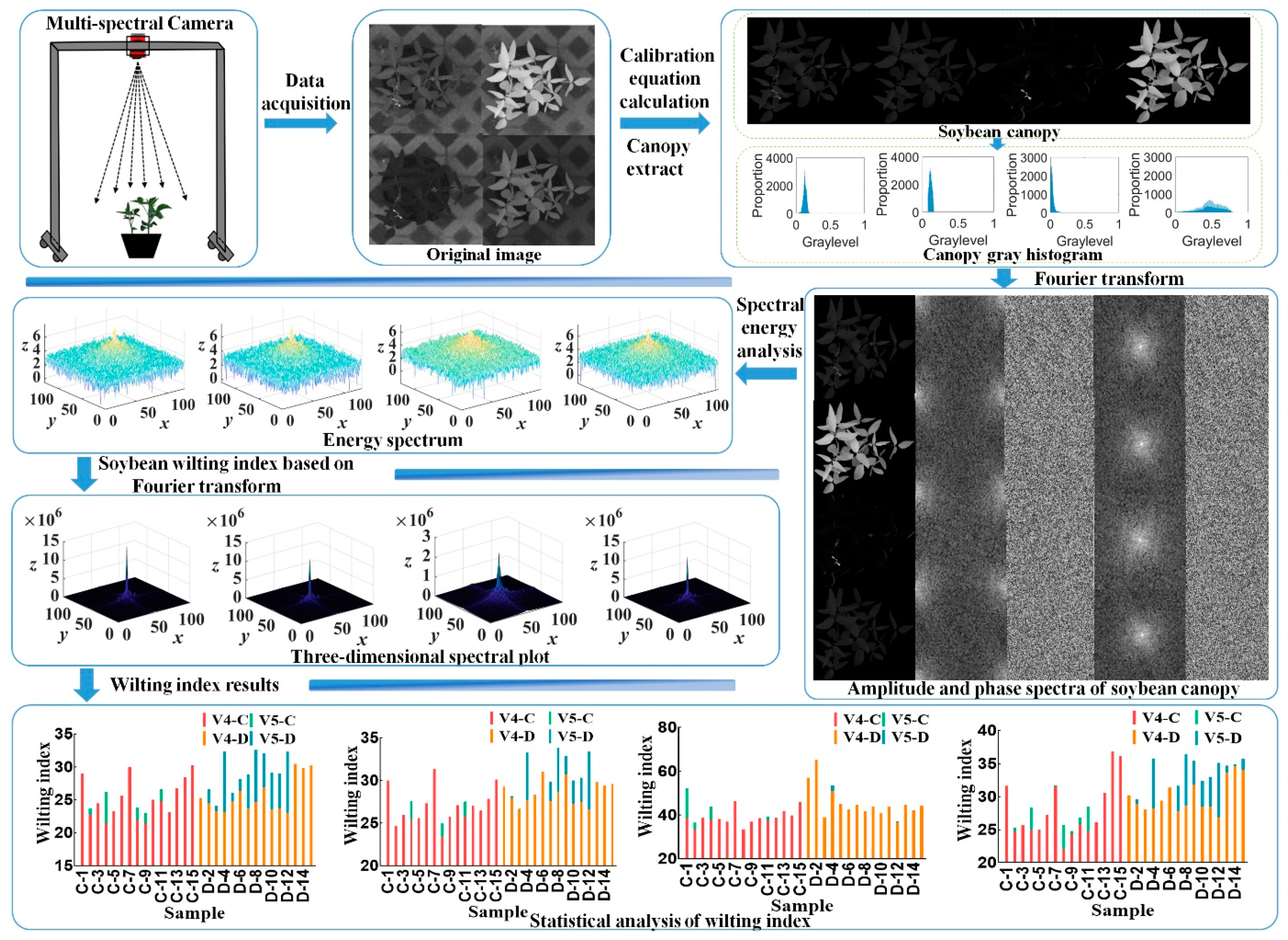

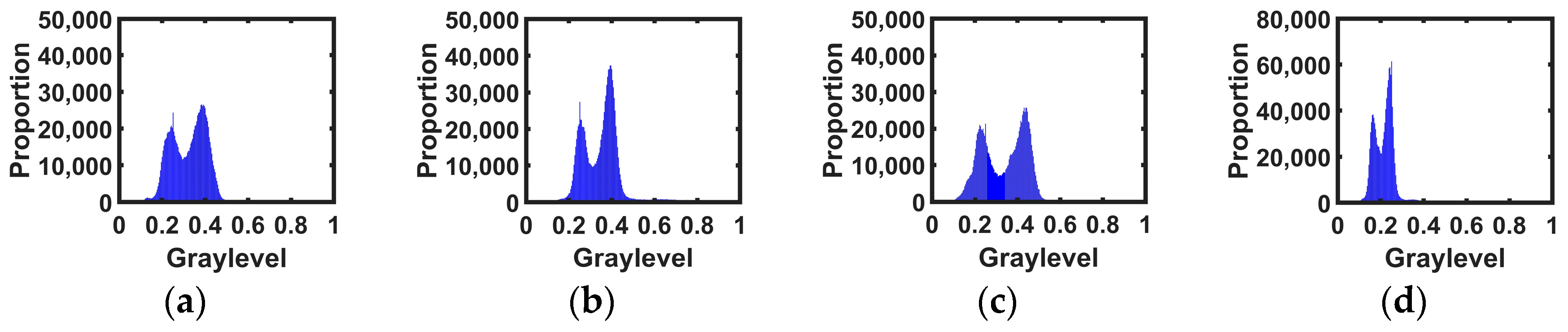
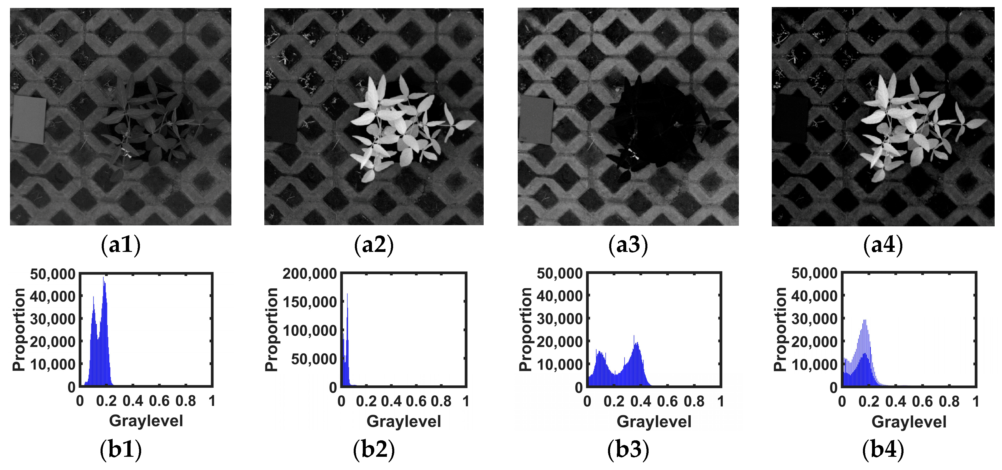
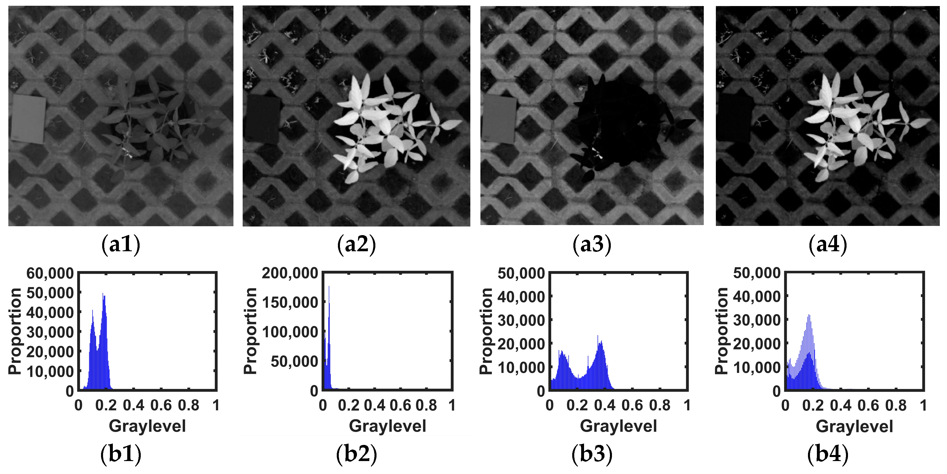
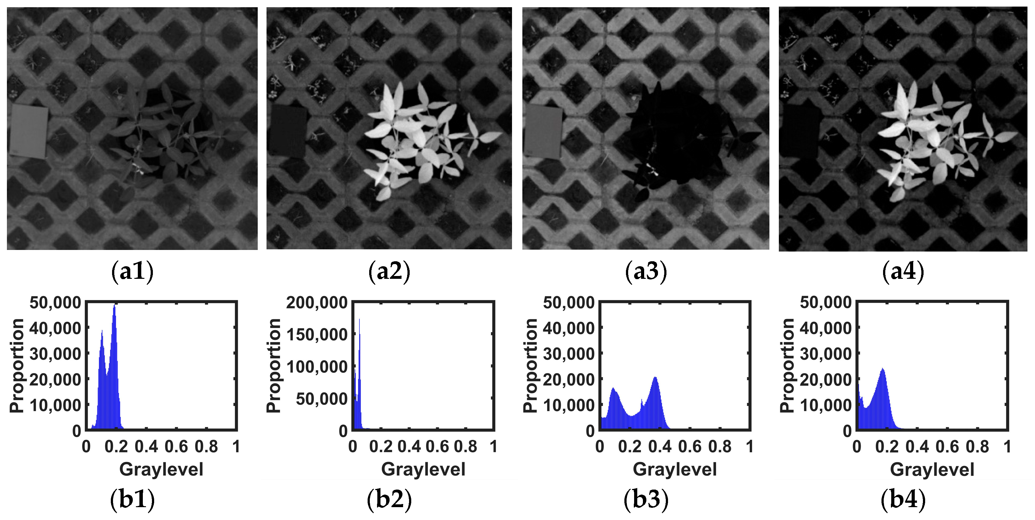
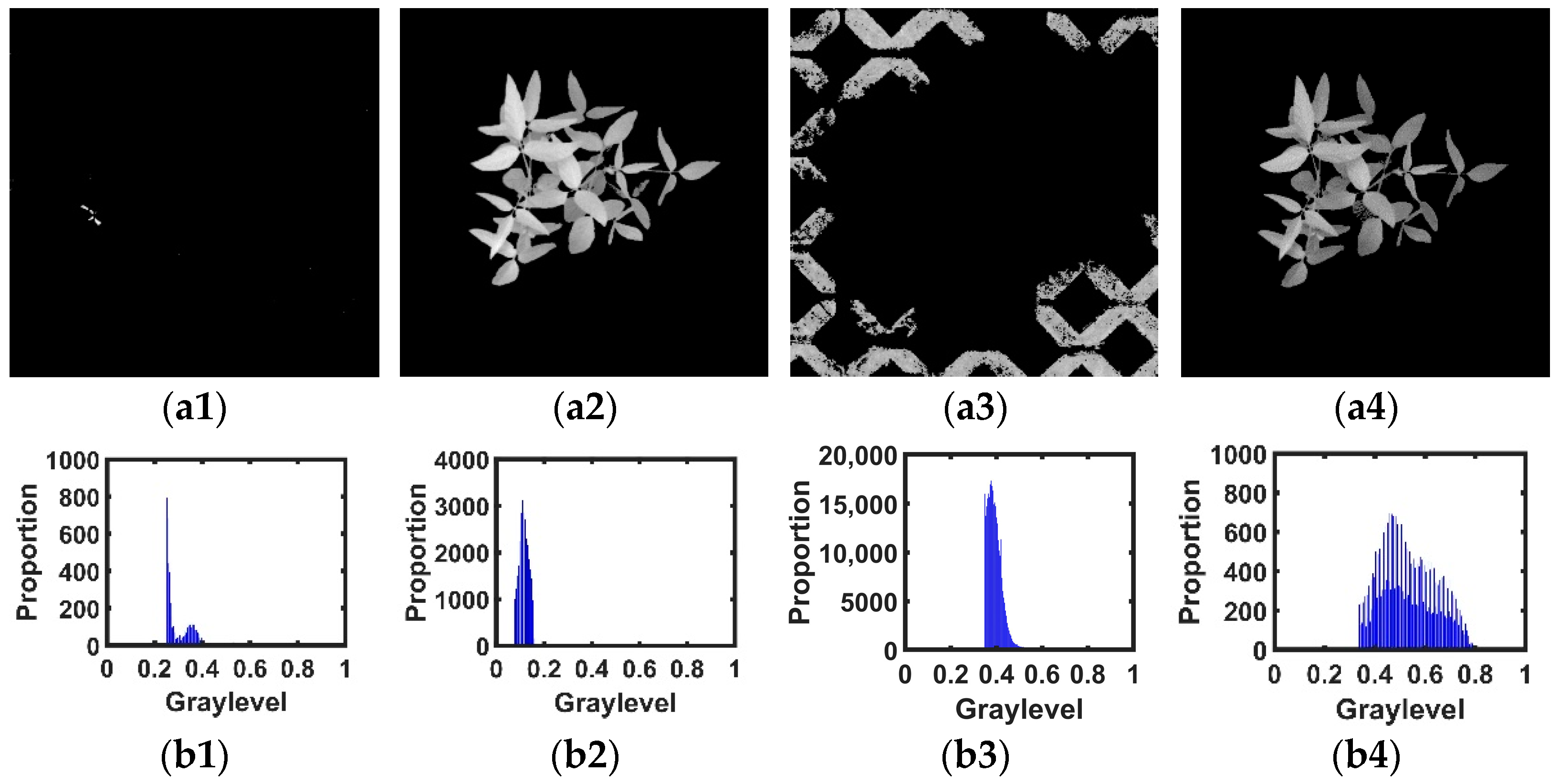
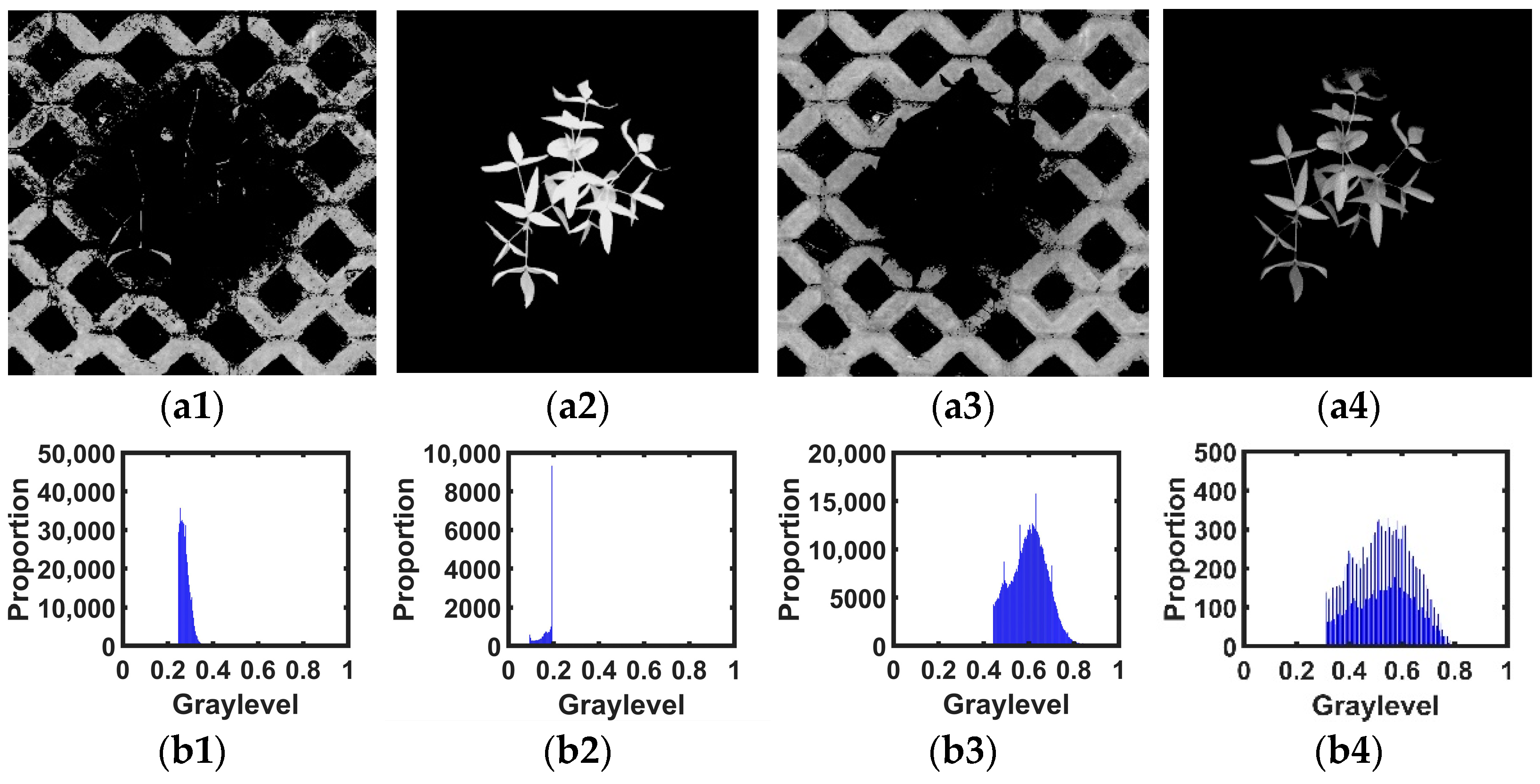
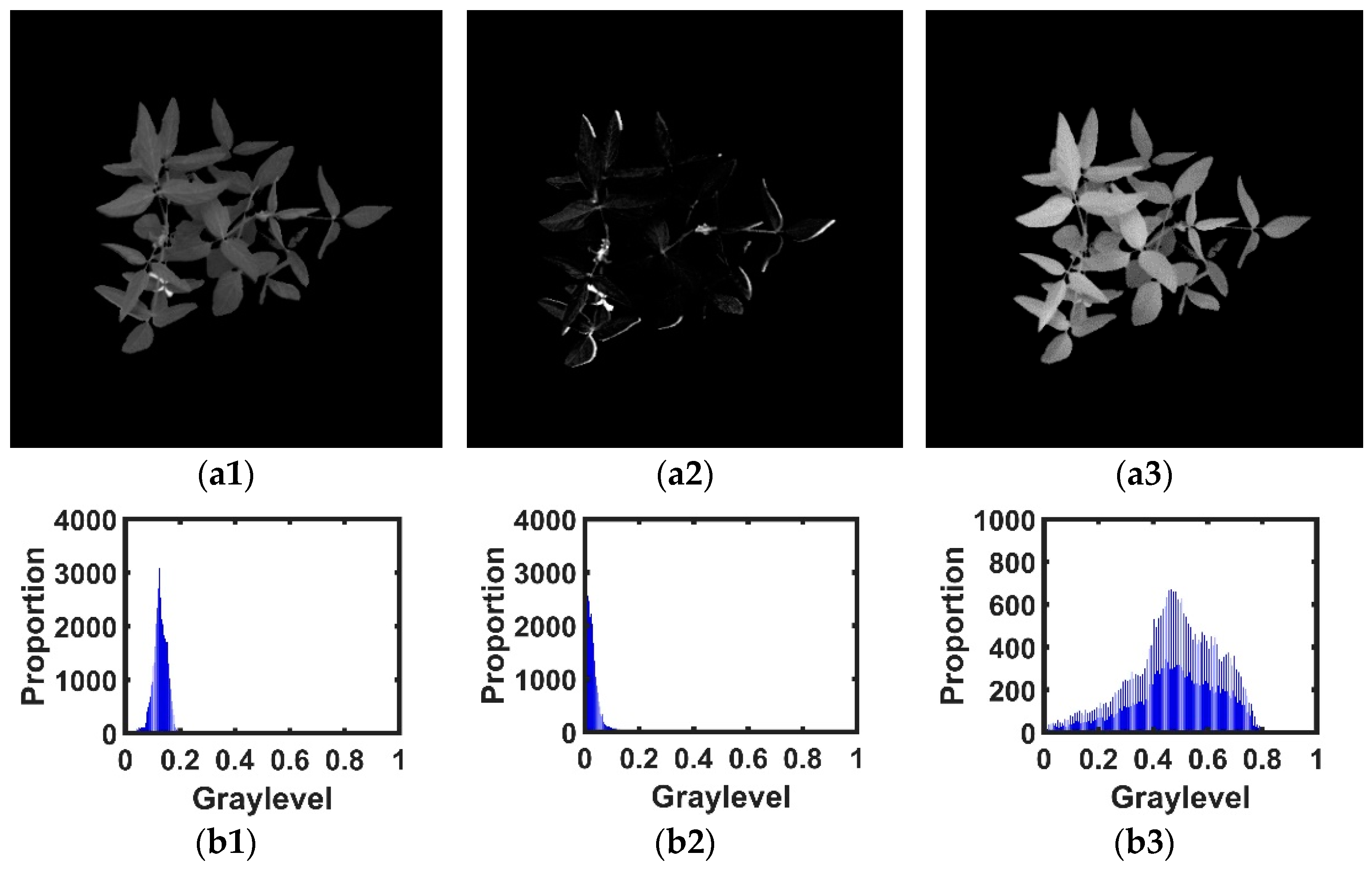
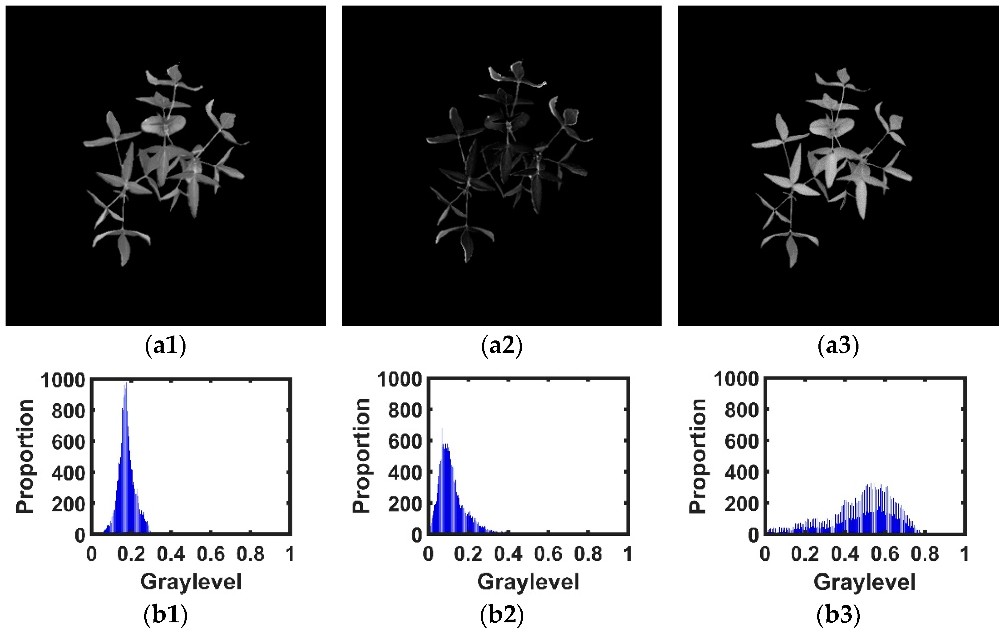
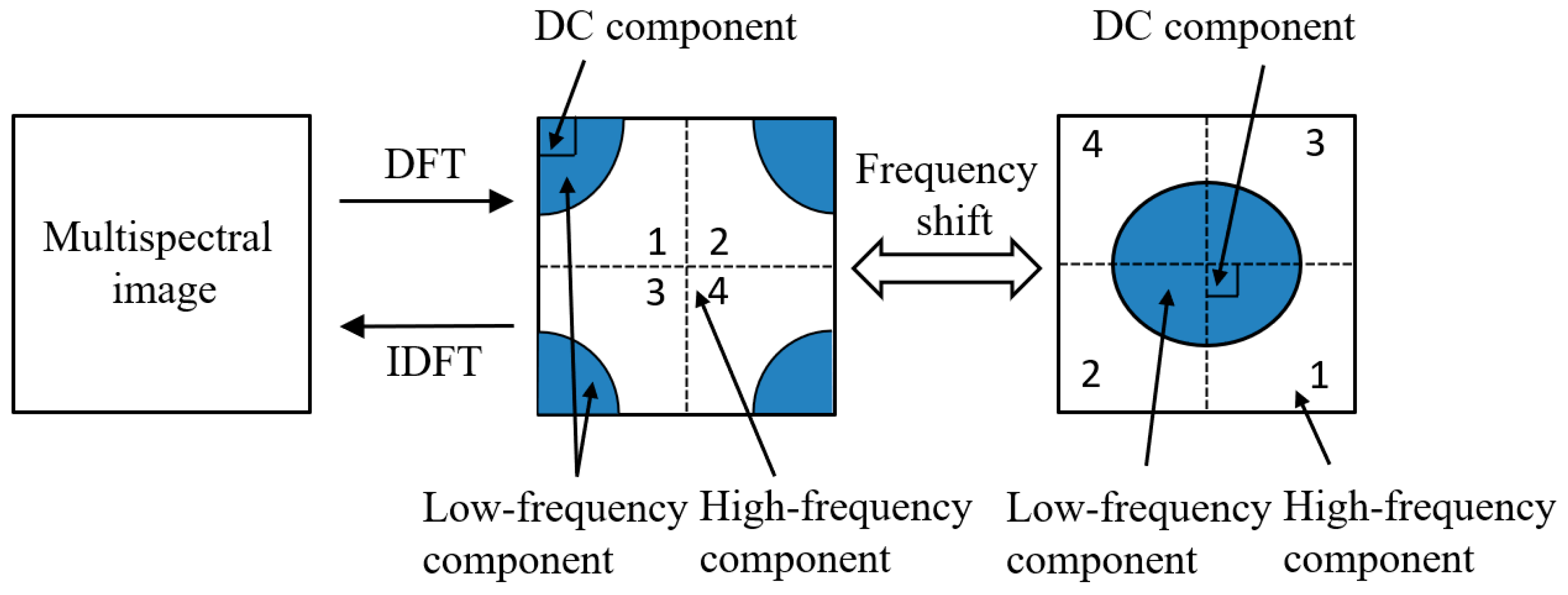
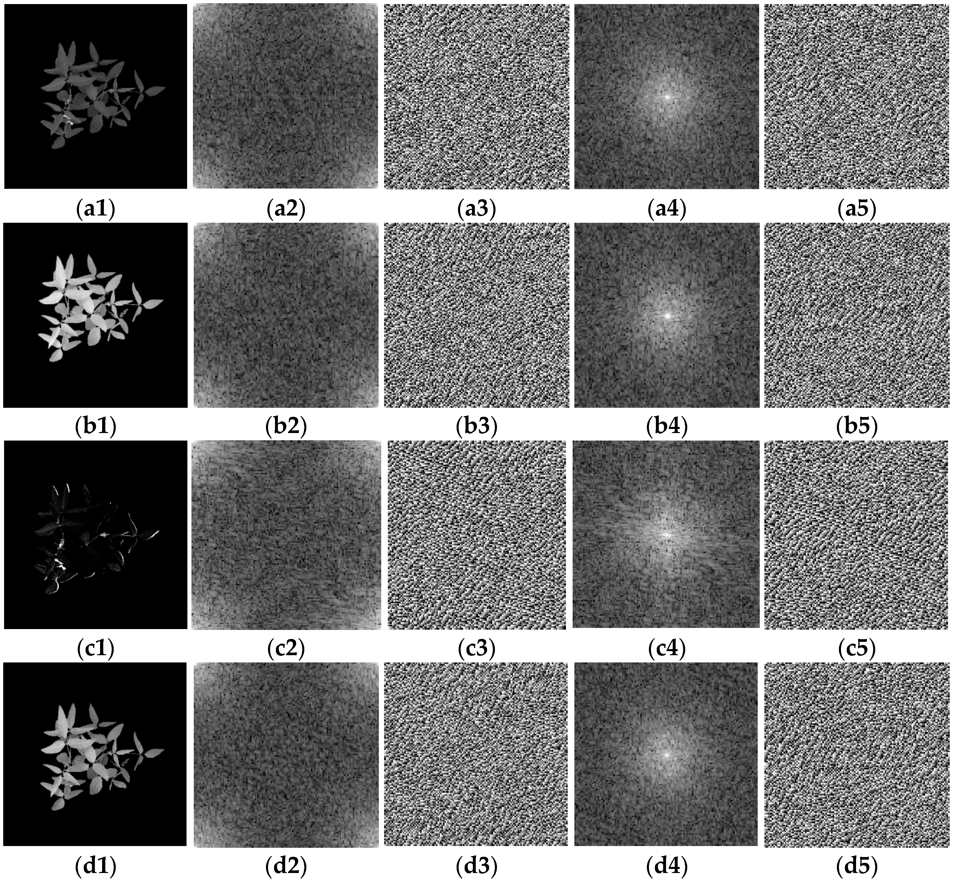
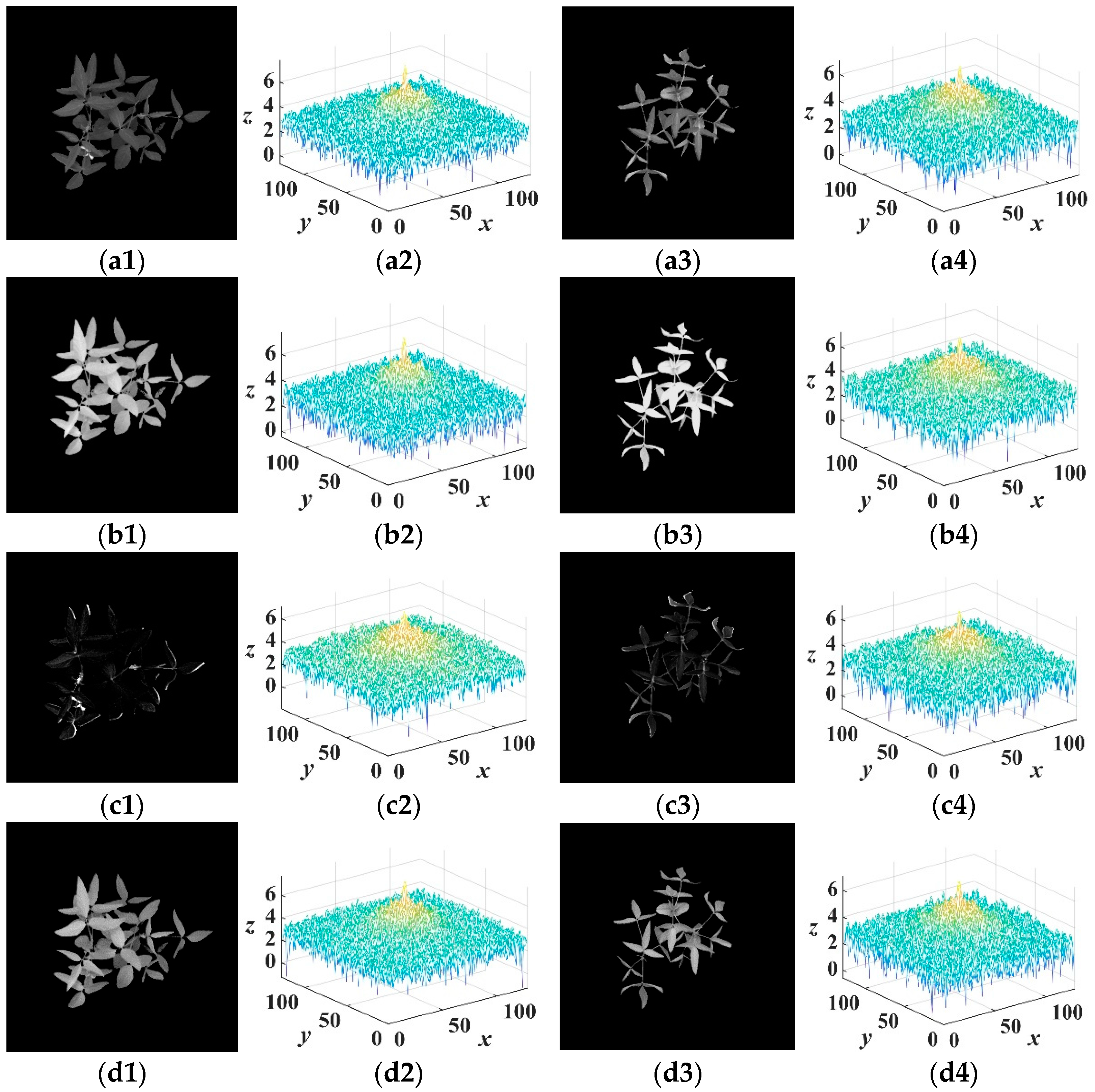
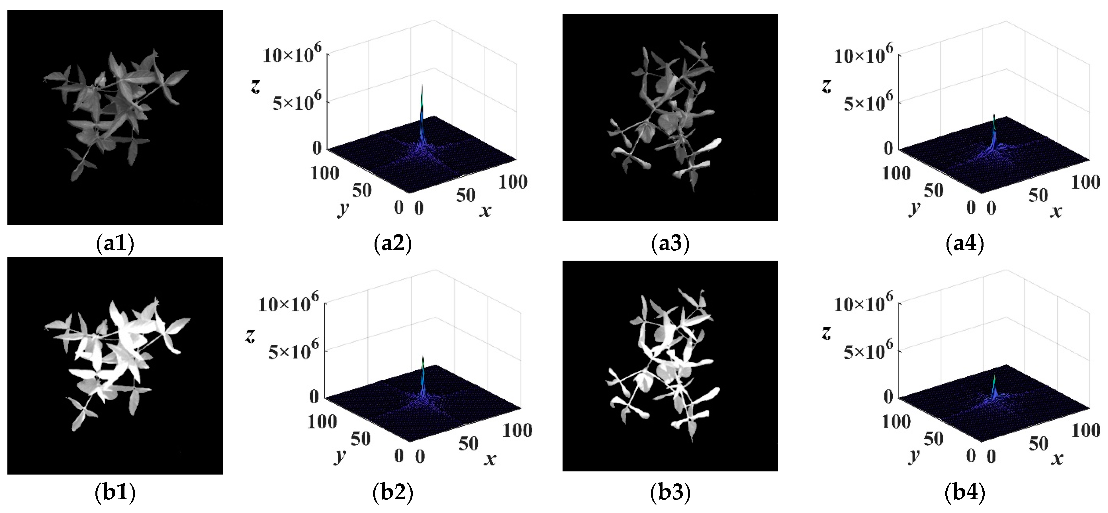
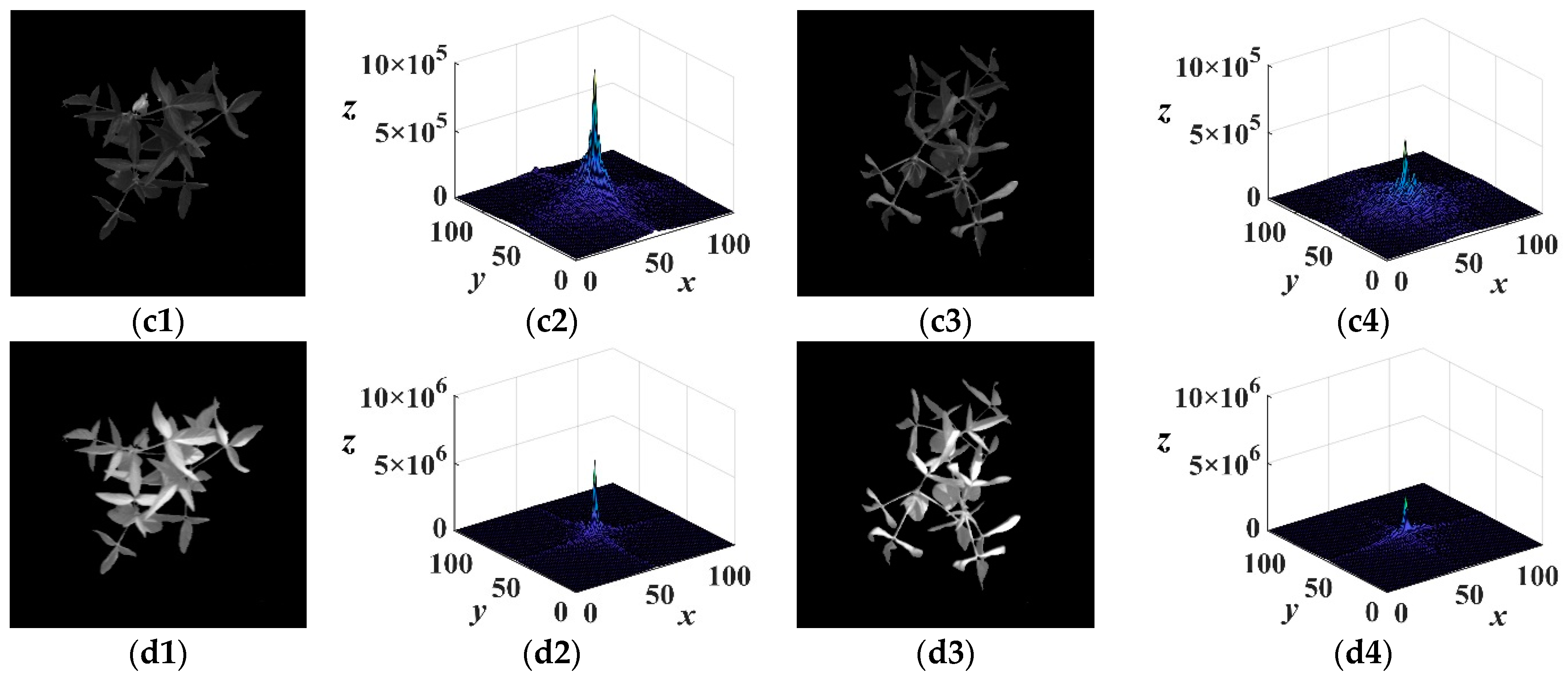
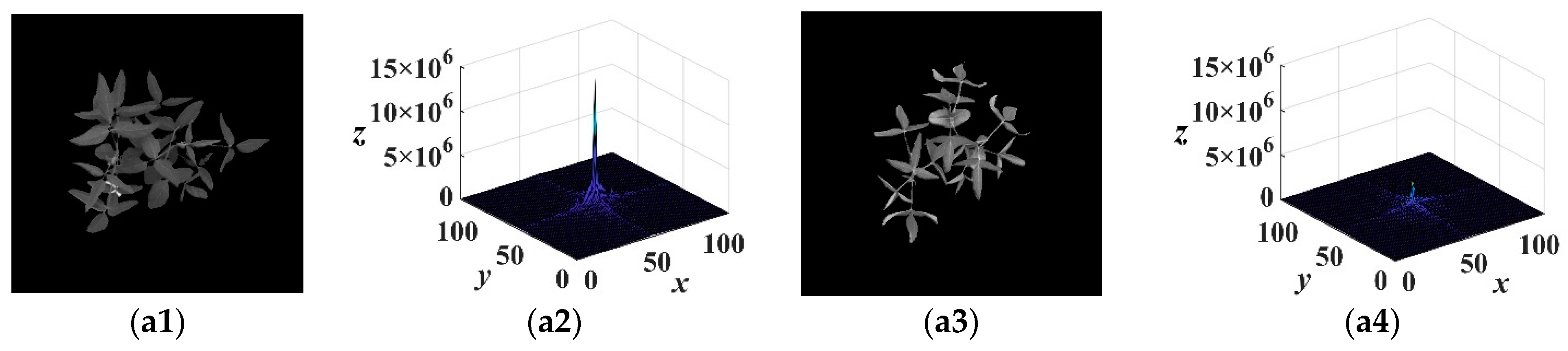
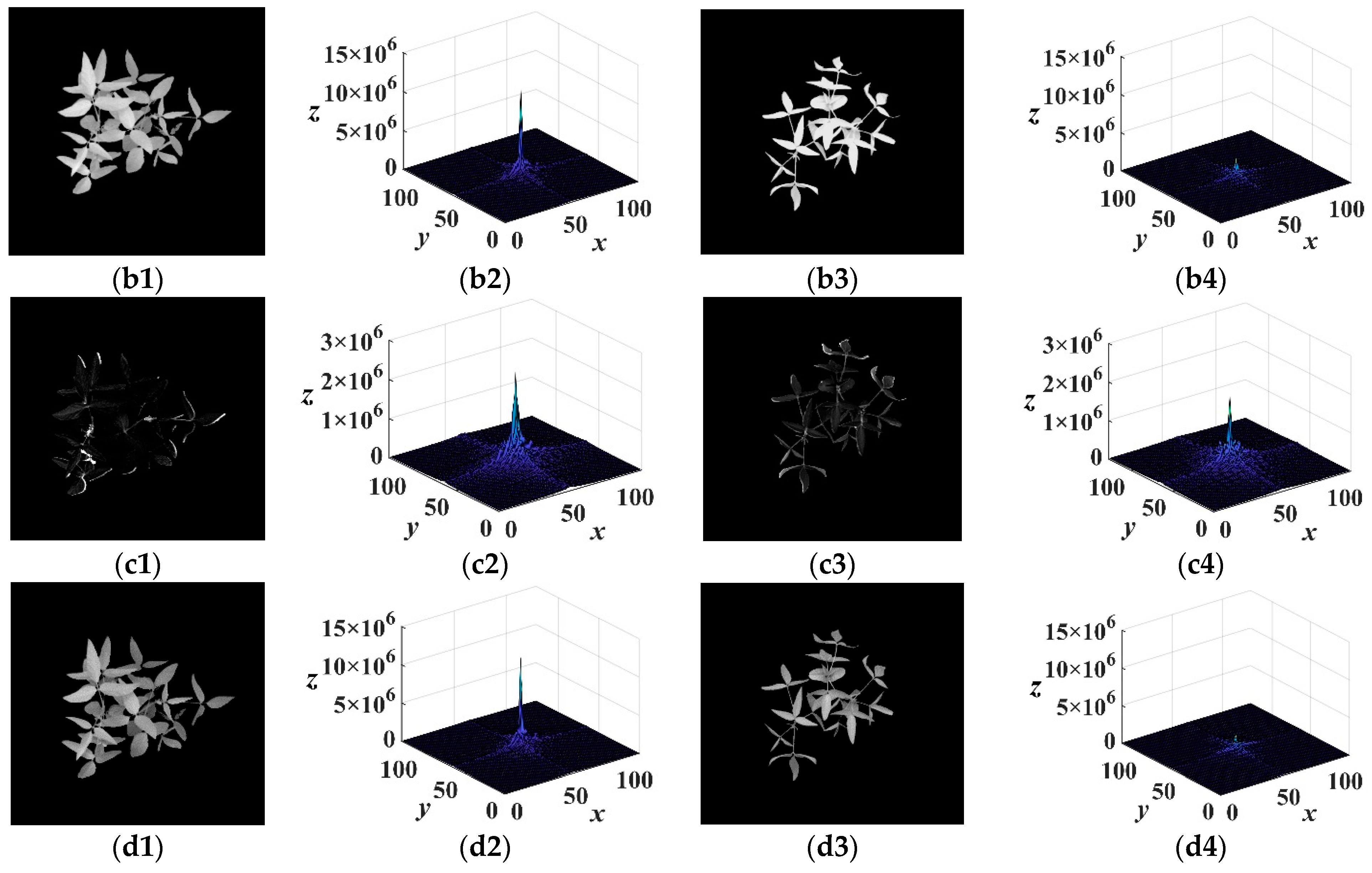
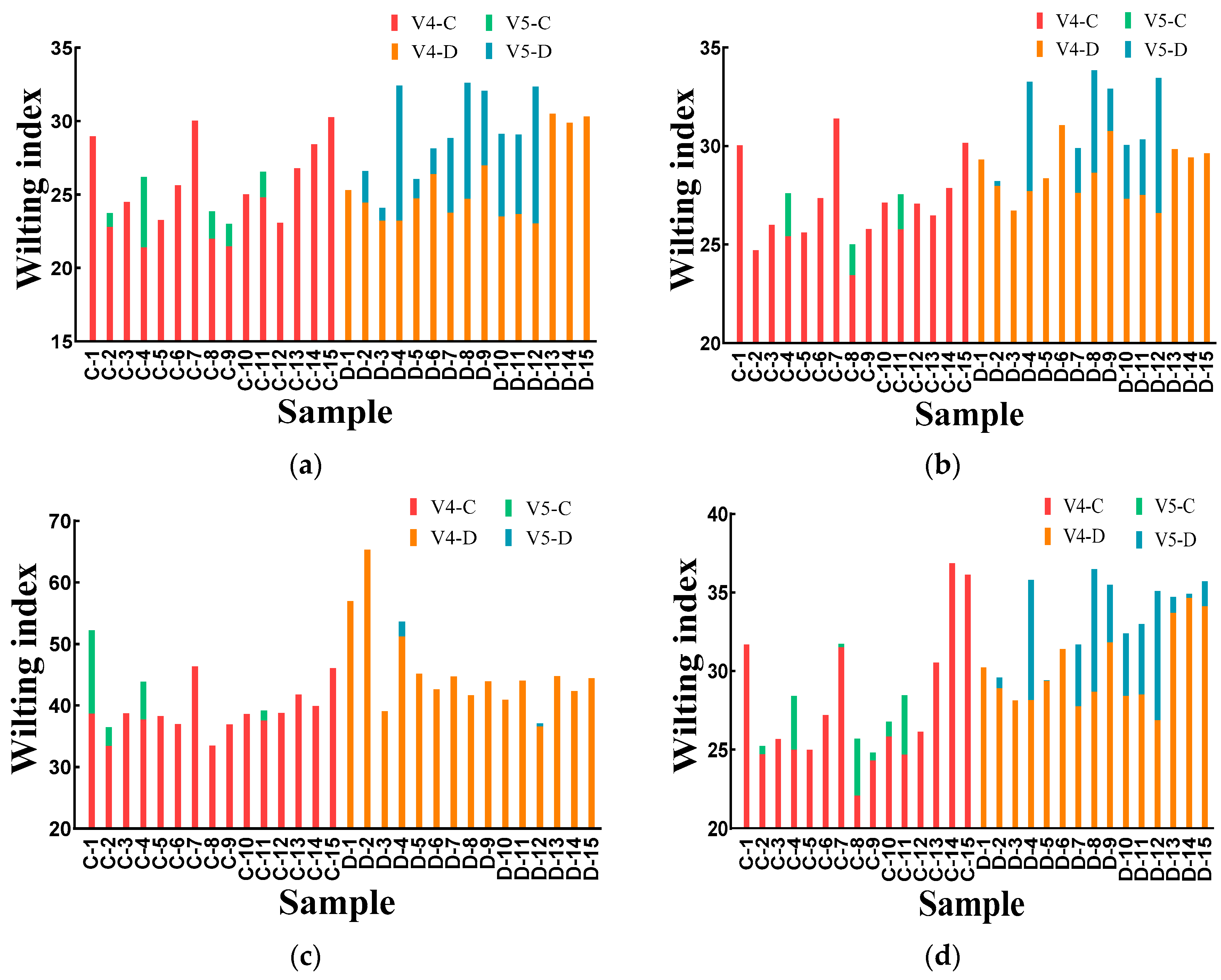
Publisher’s Note: MDPI stays neutral with regard to jurisdictional claims in published maps and institutional affiliations. |
© 2022 by the authors. Licensee MDPI, Basel, Switzerland. This article is an open access article distributed under the terms and conditions of the Creative Commons Attribution (CC BY) license (https://creativecommons.org/licenses/by/4.0/).