Monitoring Indicators for Comprehensive Growth of Summer Maize Based on UAV Remote Sensing

Abstract

Maize is one of the important grain crops grown globally, and growth will directly affect its yield and quality, so it is important to monitor maize growth efficiently and non-destructively. To facilitate the use of unmanned aerial vehicles (UAVs) for maize growth monitoring, comprehensive growth indicators for maize monitoring based on multispectral remote sensing imagery were established. First of all, multispectral image data of summer maize canopy were collected at the jointing stage, and meanwhile, leaf area index (LAI), relative chlorophyll content (SPAD), and plant height (VH) were measured. Then, the comprehensive growth monitoring indicators CGMI_CV and CGMI_CR for summer maize were constructed by the coefficient of variation method and the CRITIC weighting method. After that, the CGMI_CV and CGMI_CR prediction models were established by the partial least-squares (PLSR) and sparrow search optimization kernel extremum learning machine (SSA-KELM) using eight typical vegetation indices selected. Finally, a comparative analysis was performed using ground-truthing data, and the results show: (1) For CGMI_CV, the R² and RMSE of the model built by SSA-KELM are 0.865 and 0.040, respectively. Compared to the model built by PLSR, R² increased by 4.5%, while RMSE decreased by 0.3%. For CGMI_CR, the R² and RMSE of the model built by SSA-KELM are 0.885 and 0.056, respectively. Compared to the other model, R² increased by 4.6%, and RMSE decreased by 2.8%. (2) Compared to the models by single indicator, among the models constructed based on PLSR, the CGMI_CR model had the highest R². In the models constructed based on SSA-KELM, the R² of models by the CGMI_CR and CGMI_CV were larger than that of the models by SPAD (R² = 0.837), while smaller than that of the models by LAI (R² = 0.906) and models by VH (R² = 0.902). In summary, the comprehensive growth monitoring indicators prediction model established in this paper is effective and can provide technical support for maize growth monitoring.

1. Introduction

Maize is one of the most important crops grown globally and accounts for the highest proportion of the global cereal market. Ensuring maize production is of great significance in guaranteeing global economic development and food security [1]. The growth of maize is an important data source for early yield estimation, and its final yield can be predicted to a certain extent. Sujan Sapkota et al. [2] used a drone equipped with a multispectral camera to obtain the canopy spectral information of maize plants, and successfully monitored the growth and yield estimation of maize by using multiple growth parameters such as maize plant height, biomass, and leaf area index combined with vegetation index. Therefore, real-time and effective monitoring of field corn growth is of great significance in guiding field management [3]. In maize growth monitoring research, many parameters characterize maize growth [4,5,6,7], such as aboveground biomass, chlorophyll content, leaf area index, plant height, and leaf nitrogen content. In the study, three growth indicators, leaf area index (LAI, total plant leaf area per unit land area as a multiple of land area), relative chlorophyll content (SPAD, relative proportions of chlorophyll content in different samples), and plant height (VH, distance from the base of the plant to the top of the main stem, i.e., between the growing points of the main stem), were selected to initiate research and analysis of summer maize growth monitoring.

The leaf area index (LAI) is an important basis for characterizing the canopy structure and growth of crops, and is one of the most important parameters for evaluating crop growth conditions [8]. Ma JW et al. [9] constructed and validated a winter wheat LAI prediction model by combining four methods (GPR, artificial neural network (ANN), partial least-squares regression (PLSR), and spectral index (SI), with hyperspectral data), and the results showed the best results for ANN and GPR. Hang YH et al. [10] explored the use of spectral features, texture index, and crop cover to construct LAI estimation models through UAV remote sensing data, and the results showed that the combination of the three types of indices to construct multiple stepwise regression and artificial neural network models estimated LAI with the best accuracy. Tao HL et al. [11] used a UAV with a hyperspectral camera, and used stepwise regression analysis (SWR) and PLSR methods to predict AGB and LAI using vegetation index, red edge parameters, and their combinations, respectively. The results showed that the PLSR algorithm had the best effect in predicting AGB and LAI by combining the vegetation index with the red edge parameters. Chlorophyll (SPAD) is the main pigment that converts light energy into chemical energy and is the driving force behind photosynthesis in plants [12]. Qiao L et al. [13] utilized multispectral remote sensing images of maize captured by drones during the tasseling stage. They observed a significant linear correlation between near-ground vegetation indices and maize canopy chlorophyll content under medium and low crop coverage. For high coverage, a noticeable nonlinear correlation emerged, and the model for monitoring chlorophyll content, established based on partial least-squares regression (PLSR), demonstrated the best performance. Guo Y [14] and team identified optimal combinations of drone spectral indices and texture indices using the SRM model. Applying support vector machine (SVM) and random forest (RF) models, they estimated maize SPAD values, with the SVM model yielding the most optimal predictive results. Plant height (VH), as an important indicator of crop growth, can be used to indirectly obtain crop biomass [15], and can also be used to predict crop yield in conjunction with vegetation index and canopy cover [16]. Bending et al. [17] obtained visible-light data of barley based on a UAV-mounted digital camera. By constructing a CMS, they realized the accurate extraction of crop height and established a barley plant height estimation model. Xu YF et al. [18] constructed 22 multispectral vegetation indices with image spectral reflectance features, and selected three different machine learning algorithms to establish a plant height monitoring model for winter wheat. The results showed that the optimal prediction model for plant height was the MLR-VH model. Under normal circumstances, a single growth indicator characterizes the physiological information status of crops in a certain aspect. The data belong to the ‘point’ data in essence, and to a certain extent, they cannot represent the overall growth situation of crops, the use of multiple indicators, and the relationship between them to establish a comprehensive growth monitoring indicator (CGMI), which is of practical significance for remote sensing monitoring of crop growth.

Comprehensive growth monitoring indicators can be modeled according to different assignment methods, and the commonly used assignment method is the equalization method. Pei HJ et al. [19] synthesized five indicators reflecting wheat growth, including leaf area index, leaf chlorophyll content, plant nitrogen content, plant water content, and biomass, into a single growth indicator according to equal weights, and combined wheat growth by combining with partial least-squares regression, and achieved a high-precision model. This method did not take into account the contribution of a single indicator to the integrated growth monitoring indicator and simply constructed each indicator into a composite indicator according to equal weights. Although the above studies have good predictive capabilities, most of them are limited to using a single growth indicator to predict crop growth, or simply constructing a comprehensive growth indicator without considering the contribution of each indicator to crop growth, which makes them constructed from the prediction model has certain limitations. Considering the different degrees of importance of each indicator in the comprehensive growth monitoring indicators and the non-uniformity of the scale of each indicator, the coefficient of variation method and the CRITIC weighting method were used to try to construct the comprehensive growth monitoring indicators (CGMI).

In the study, we used summer maize multispectral image data to establish a crop growth monitoring model, and comparatively analyzed the correlation between comprehensive growth monitoring indices and individual indices and vegetation index. The main objectives include: (1) use of the coefficient of variation method and CRITIC weighting method to weight chlorophyll content, leaf area index, and plant height according to their contribution to the overall growth, and construct comprehensive growth monitoring indices respectively; (2) analysis of the correlation of comprehensive growth monitoring indicators and individual indicators with vegetation indices; (3) use of the PLSR and SSA-KELM algorithms to construct a comprehensive growth monitoring indicator prediction model, followed by analysis in comparison with a single growth indicator prediction model.

2. Materials and Methods

2.1. Overview of the Experimental Area

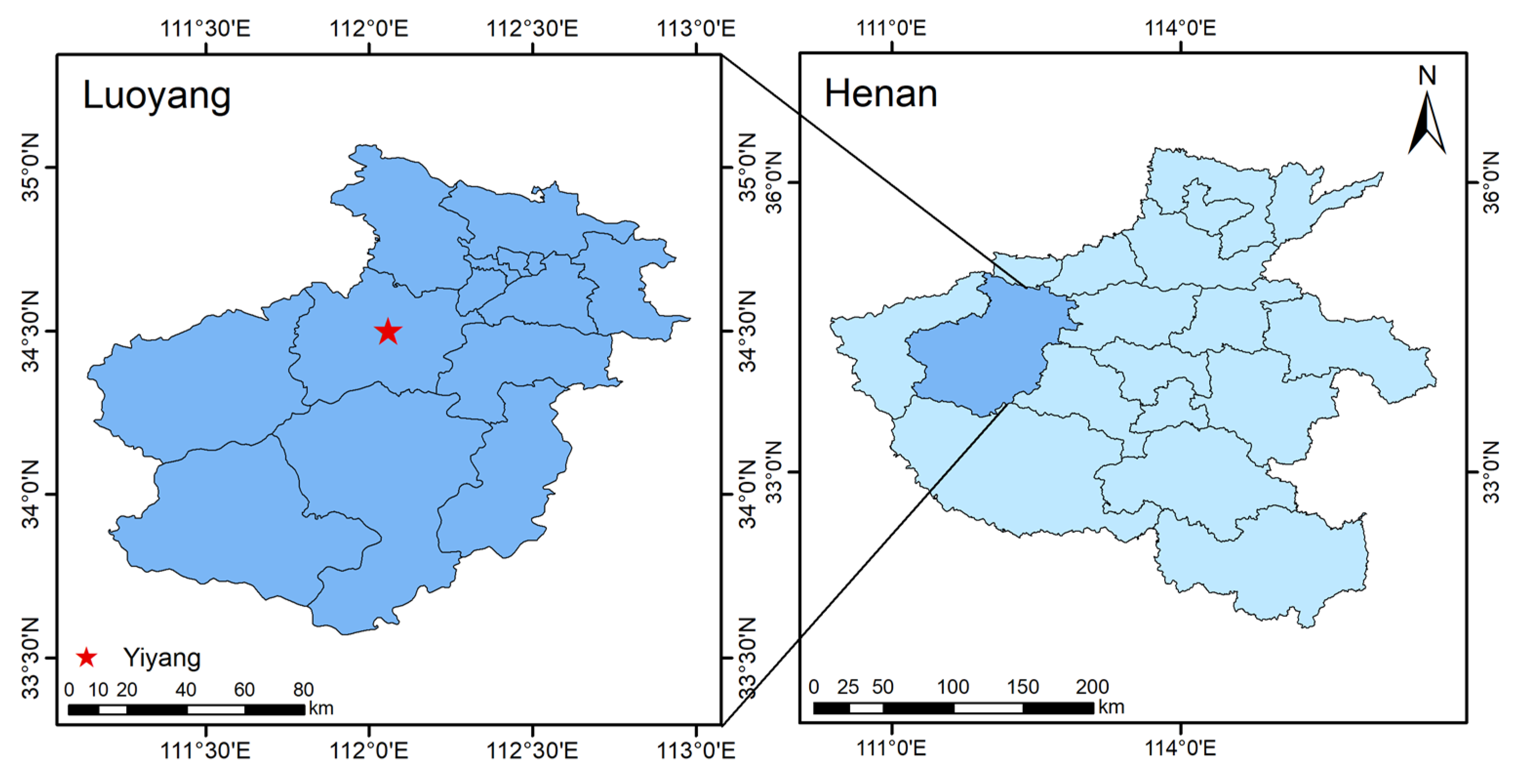
The experimental area was situated in China’s first tractor company limited intelligent agriculture demonstration farm in Yiyang County, Luoyang City, Henan Province, China, at coordinates 112°37′11.72″ E, 34°47′79.03″ N, belonging to the temperate continental monsoon-type climate. The area where the geographical coordinates are located is shown in Figure 1. The terrain in the experimental field was flat. The maize variety in this experiment was Zheng Dan 958, which was planted in rotation with wheat. The planting density is 67,000 plants m⁻², the row spacing is 0.6 m, and the plant spacing is 0.2 m. Its management methods, such as irrigation, fertilization, pest, and weed control, were the same as those of local conventional farmland.

2.2. UAV Data Acquisition and Preprocessing

This study utilized a DJI Phantom 4 drone (DJI, Shenzhen, China) to collect multispectral remote sensing data of summer maize, equipped with an integrated multispectral imaging system consisting of one visible-light camera and five multispectral cameras (blue, green, red, red edge, and near-infrared). The experiment took place on 22 July 2022, from 10:00 to 12:00 during the summer maize jointing stage, with stable light intensity, clear weather, and no wind.

Before image acquisition, flight routes were planned using mapping software (DJI Terra, V3.9.4, DJI, Shenzhen, China), and spectral image collection followed the planned routes. The drone flew at a height of 70 m, with the sensor lens pointing vertically downward and an 85% overlap rate in both longitudinal and lateral directions. The flight direction was north-south, with a speed of 3.5 m/s.

For reflectance calibration, a calibration reflectance panel was placed on the ground in the experimental area before and after image acquisition. The drone, manually controlled, hovered 2 m directly above the calibration panel to capture spectral images, obtaining standard reflectance values for the test.

Import the gathered multispectral images into Pix4D Mapper software (from Pix4D, V4.4.12, Lausanne, Switzerland) for preprocessing to derive the reflectance spectrum of summer corn within the sampling point ROI region (illustrated as the box in Figure 2). The primary steps encompass (1) ortho-image processing; (2) calibration using reflectance board DN values, generating stitched images; (3) geometric correction with concurrently obtained high-definition digital images as references; (4) choosing the necessary ROI region pertinent to this study; (5) deriving the average reflectance spectrum within the ROI, representing the summer corn’s reflectance spectrum within that specific ROI region. For this study, 20 experimental ROI regions, each measuring 10 m × 5 m, are chosen based on growth gradients. Of the data, 70% is designated as the training set (70 plants of maize), while the remaining 30% forms the validation set (30 plants of maize).

2.3. Field Data Acquisition

Growth indicators are time-sensitive [21]. Ground-truthing data, mainly including relative chlorophyll content, leaf area index, and plant height, were synchronously collected on the same day that summer maize multispectral remote sensing data were acquired.

(1)

Measurement of Relative Chlorophyll Content

In this experiment, a portable SPAD-502Plus chlorophyll meter (Konica Minolta, Tokyo, Japan) was used for SPAD determination. Five maize plants were selected in each experimental area according to the five-point sampling method, avoiding leaf veins to collect the SPAD values of the three parts of the ear leaves of each maize plant, the root, the middle of the leaf, and the tip of the leaf. Each part was repeated twice, and the average of the six times’ data was taken as the SPAD value of the plant [22]. The mean SPAD value of 5 plants in the experimental area was calculated as the relative chlorophyll content of maize plants in that area.

(2)

Determination of Leaf Area Index

In this experiment, leaf area index data were collected using the aspect ratio method. Measure summer maize leaf length $L_{ij}$ and maximum leaf width $B_{ij}$ with a tape measure. Five maize plants were selected from each experimental area according to the five-point sampling method, and the $L_{ij}$ and $B_{ij}$ of their leaves were measured, and each part was repeated three times to take the average value [23]. The mean LAI value of five plants in the experimental area was calculated as the LAI of maize plants in the area. The LAI calculation formula is as follows:

$$\mathrm{L}\mathrm{A}\mathrm{I}=\alpha \times \rho \frac{{\sum }_{i=1}^m{\sum }_{j=1}^n\left(L_{ij}\times B_{ij}\right)}{m}$$

(1)

where $\alpha$ is the maize leaf area conversion factor with a value of 0.75, $\rho$ is the planting density (plants m⁻²), $n$ is the total number of leaves (pieces) of the $j$th plant, and $m$ is the number of plants measured.

(3)

Maize Height Measurement

Five maize plants were selected in each ROI area according to the five-point sampling method, and the vertical distance from the ground to the highest point of the plant was measured physically using a tape measure with the plant’s leaves naturally spread. Measurements were repeated three times for each plant to take the average value. The average heights of the five maize plants in the experimental area were taken as the plant height of the maize in that area.

2.4. Comprehensive Growth Indicator Construction

Based on the importance of relative chlorophyll content, leaf area index, and plant height in the comprehensive growth monitoring indicator of summer maize, the Comprehensive growth monitoring indicator (CGMI) of maize was constructed. For this reason, in this study, the CRITIC weighting method was used in this study to determine the weights of the three indicators, and the weights of LAI, SPAD, and VH were A, B, and C. This led to the establishment of the comprehensive growth monitoring indicator CGMI_CR.

The CRITIC weighting method is an objective method of assigning weights based on the volatility of data [24]. Its basic idea lies in two indicators, which are volatility (contrast strength) and conflict (correlation) indicators. Volatility is expressed using the standard deviation. If the larger the standard deviation of the data indicates greater volatility, the higher the weight will be. Conflict is expressed using the correlation coefficient table. If the value of the correlation coefficient between the indicators is larger, it means that there is more similarity between the indicators, and the smaller the conflict, then its weight will be lower.

(1)

Data Normalization

To eliminate the influence of different scales on the evaluation results, it is necessary to normalize the indicators. The normalization formula is as follows:

$${X^{\prime }}_{ij}=\frac{X_{ij}-X_{jmin}}{X_{jmax}-X_{jmin}}$$

(2)

$$U_j=\left(X_{1j}^{\prime },X_{2j}^{\prime },X_{3j}^{\prime }\dots \dots X_{ij}^{\prime }\right)$$

(3)

where $X_{ij}$ denotes the value of the $j$th evaluation indicator for the $i$th sample, $X_{jmin}$ denotes the minimum value in the $j$th indicator, $X_{jmax}$ denotes the maximum value in the $j$th indicator, and $U_j$ denotes the data normalized to the $j$th indicator.

(2)

Calculation of Indicator Volatility

In the CRITIC weighting method, a larger standard deviation indicates that the indicator is more volatile and more informative, and more weight should be given to the indicator.

$${\overline{X}}_j=\frac{1}{n}\sum _{i=1}^n{X}_{ij}$$

(4)

$$S_j=\sqrt{\frac{{\sum }_{i=1}^n{\left(X_{ij}-{\overline{X}}_j\right)}^2}{n-1}}$$

(5)

where ${\overline{X}}_j$ denotes the mean of the $j$th indicator, and $S_j$ denotes the standard deviation of the $j$th indicator is the volatility of that indicator.

(3)

Calculation of Conflicting Indicators

The conflict between indicators is expressed using the correlation coefficient; the stronger the correlation between an indicator and other indicators, the less conflict there is between the indicator and other indicators, reflecting more of the same information, and the more repetitive the content of the evaluation that can be embodied, which to a certain extent weakens the intensity of the evaluation of the indicator, and the weight assigned to the indicator should be reduced.

$$R=\frac{{\sum }_{j,k=1}^P\left(x_{ij}-{\overline{x}}_j\right)\left(x_{ik}-{\overline{x}}_k\right)}{\sqrt{{\sum }_{j=1}^P{\left(x_{ij}-{\overline{x}}_j\right)}^2{\sum }_{k=1}^P{\left(x_{ik}-{\overline{x}}_k\right)}^2}}$$

(6)

$$A_j=\sum _{i=1}^P\left(1-r_{ij}\right)$$

(7)

where $R$ denotes the correlation matrix of the indicator, $j,k$ denote the $j$th indicator and the $k$th indicator, $r_{ij}$ denotes the correlation coefficient between the $i$th indicator and the $j$th indicator, and $P$ denotes the number of indicators.

(4)

Calculation of the Information Content of the Indicator

$$C_j=S_j\times A_j$$

(8)

(5)

Calculation of Objective Weights for Indicators

$$W_j=\frac{C_j}{{\sum }_{j=1}^P{C}_j}$$

(9)

where $W_j$ denotes the weight of the $j$th indicator in the whole evaluation system, and $P$ denotes the number of indicators.

(6)

Comprehensive Growth Monitoring Indicator CGMI_CR

The CRITIC weight method was used to derive A, B, and C as 0.331, 0.390, and 0.279, respectively, and the comprehensive growth monitoring indicator CGMI_CR was constructed. The expression of CGMI_CR is as follows:

$$\mathrm{C}\mathrm{G}\mathrm{M}{\mathrm{I}}_{\mathrm{C}\mathrm{R}}=0.331U_1+0.390U_2+0.279U_3$$

(10)

where $U_1$ is the normalized LAI value, $U_2$ is the normalized SPAD value, and $U_3$ is the normalized VH value.

2.5. Selection of Vegetation Indices

In the initial stage of the study, the correlation analysis between a single band and the maize growth indicator showed that the correlation between the single band and the maize growth indicator was low, which was similar to the results of previous studies [25,26]. Therefore, the vegetation index was used to predict the growth of maize. The vegetation index (VI) changes through the combination of reflectance in different bands, which weakens the interference of background and other factors on the spectral characteristics of vegetation to a certain extent, and helps to improve the accuracy of remote sensing data to express crop growth. [27]. To better reflect the information contained in CGMI, this study extracted the spectral reflectance of 20 ROI regions from the spliced raw images and constructed vegetation indices by linear or nonlinear combinations. Eight vegetation indices with high relevance and wide application were selected: Green Ratio Vegetation Index (GRVI), Green Optimal Soil-Adjusted Vegetation Index (GOSAVI), Optimal Vegetation Index (VIopt), Normalized Difference Vegetation Index (NVI), Green Difference Vegetation Index (GDVI), Ratio Vegetation Index (RVI), Normalized Difference Vegetation Index (NDVI), Vegetation Index (RVI), Green Normalized Difference Vegetation Index (GNDVI), and Canopy Chlorophyll Content Index (CCCI). The formula for calculating the vegetation indices is shown in

Table 1. Vegetation indices and its calculation formula [20].

Vegetation Indices	Equation	References
GOSAVI	$\left(1+0.16\right)\times \left(\mathrm{N}\mathrm{I}\mathrm{R}-\mathrm{R}\mathrm{E}\right)/\left(\mathrm{N}\mathrm{I}\mathrm{R}+\mathrm{R}\mathrm{E}+0.16\right)$	Marin D B et al. [28]
GDVI	$\mathrm{N}\mathrm{I}\mathrm{R}-\mathrm{G}$	Zhou X F et al. [29]
RVI	$\mathrm{N}\mathrm{I}\mathrm{R}/\mathrm{R}$	Jiang J et al. [30]
GNDVI	$\left(\mathrm{N}\mathrm{I}\mathrm{R}-\mathrm{G}\right)/\left(\mathrm{N}\mathrm{I}\mathrm{R}+\mathrm{G}\right)$	Jiang J et al. [30]
GRVI	$\mathrm{N}\mathrm{I}\mathrm{R}/\mathrm{G}$	Motohka T et al. [31]
VIopt	$\left(1+0.45\right)\times \left(2\mathrm{N}\mathrm{I}\mathrm{R}+1\right)/\left(\mathrm{R}+0.45\right)$	Motohka T et al. [31]
NDVI	$\left(\mathrm{N}\mathrm{I}\mathrm{R}-\mathrm{R}\right)/\left(\mathrm{N}\mathrm{I}\mathrm{R}+\mathrm{R}\right)$	Deng L et al. [32,33]
CCCI	$\left(\mathrm{N}\mathrm{I}\mathrm{R}-\mathrm{R}\mathrm{E}\right)/\left(\mathrm{N}\mathrm{I}\mathrm{R}+\mathrm{R}\mathrm{E}\right)$	Shu M Y et al. [34]

Note: R is the red band, G is the green band, NIR is the near-infrared band, and RE is the red-edge band.

.

2.6. Model Construction

In this study, kernel-based extreme learning machine based on sparrow search algorithm optimization (SSA-KELM) was used to construct a comprehensive growth monitoring model.

Kernel-based extreme learning machine (KELM) is an improved algorithm based on ELM, and combined with the kernel function, KELM guarantees good generalization ability and faster learning speed based on retaining the advantages of ELM to improve the prediction performance of the model [35]. The predictive performance of KELM is significantly influenced by the regularization coefficient C and kernel function parameter S. Inadequate parameter optimization ability and poor local search capabilities can result in convergence on local optima, leading to low prediction accuracy. The SSA-KELM model optimizes the regularization coefficient C and kernel function parameter S using the sparrow search algorithm, enhancing the model’s predictive capability. To further select the regularization coefficient C and kernel function parameter S, the fitness function is designed as the training set’s mean squared error (MSE):

$$\mathrm{M}\mathrm{S}\mathrm{E}=\frac{1}{n}{\sum }_{i=1}^n{\left(y-x\right)}^2$$

(11)

$$fitness=argmin\left(\mathrm{M}\mathrm{S}{\mathrm{E}}_{pridect}\right)$$

(12)

where $x$ is the estimated value, $y$ is the measured value, and $n$ is the number of samples.

The fitness function selects the post-training MSE. A smaller MSE indicates a higher alignment between predicted and original data. The final optimization yields the best regularization coefficient C and kernel function parameter S. Using these optimized values, the network is trained on the testing dataset [20]. The flowchart of the SSA-KELM algorithm is shown in Figure 3.

2.7. Experimental Comparison Methods

2.7.1. Coefficient of Variation Method

The coefficient of variation method was selected as the comparison method of the CRITIC weight method. The coefficient of variation method is based on the evaluation of the degree of variation of the indicator value reflected in the amount of information to determine the weight of the indicator. That is, the weight of the indicator with the changes in the value of the indicator changes is a dynamic and objective method of assigning weights, and the results of its ascertainment of the weight are not subject to the influence of the outline [36]. In this study, the coefficient of variation method was used as the comparison method of the CRITIC weight method, and the weights of LAI, SPAD, and VH were determined to be A, B, and C, respectively, and a comprehensive growth monitoring indicator CGMI_CV was established.

(1)

The data normalization process is the same as the CRITIC weight method;

(2)

Calculation of the coefficient of variation.

$${\overline{X}}_j=\frac{1}{n}\sum _{i=1}^n{X}_{ij}$$

(13)

$$S_j=\sqrt{\frac{{\sum }_{i=1}^n{\left(X_{ij}-{\overline{X}}_j\right)}^2}{n-1}}$$

(14)

$$V_j=\frac{S_j}{{\overline{X}}_j}$$

(15)

where ${\overline{X}}_j$ denotes the mean value of the $j$th indicator, $S_j$ denotes the standard deviation (mean square error) of the $j$th indicator, and $V_j$ denotes the coefficient of variation of the $j$th indicator.

(3)

Calculation of Indicator Weights

$$W_j=\frac{V_j}{{\sum }_{i=1}^P{V}_j}$$

(16)

where $W_j$ denotes the weight of the $j$th indicator in the whole evaluation system and $P$ denotes the number of indicators.

(4)

Comprehensive Growth Monitoring Indicator CGMI_CV

The coefficient of variation method was used to derive A, B, and C as 0.440, 0.202, and 0.358, respectively, and the comprehensive growth monitoring indicator CGMI_CV was constructed, and the expression of CGMI_CV is as follows:

$$\mathrm{C}\mathrm{G}{\mathrm{M}\mathrm{I}}_{\mathrm{C}\mathrm{V}}=0.440U_1+0.202U_2+0.358U_3$$

(17)

where $U_1$ is the normalized LAI value, $U_2$ is the normalized SPAD value, and $U_3$ is the normalized VH value.

2.7.2. Partial Least-Squares Regression (PLSR) Method

PLSR is a technique aimed at identifying the optimal fitting function for a dataset by minimizing the sum of squared errors. It blends statistical methods like correlation analysis, principal component analysis, and multiple linear regression, effectively addressing issues related to data covariance [37]. Xie P et al. [38] used PLSR and PSO-SVM algorithms to compare and establish a hyperspectral quantitative inversion model of soil selenium content. Fu HY et al. [39] used PLSR, SVM, RF, and other modeling methods to construct the estimation models of relative chlorophyll content, leaf area index, and leaf relative water content of ramie, respectively, and proposed a more suitable dynamic monitoring method for physical and chemical traits of ramie in the field. In comparison to multivariate linear regression algorithms, PLSR can establish a multivariate linear model when the independent variables have multicollinearity and a limited number of sample points, ensuring predictive accuracy. In contrast to principal component analysis, partial least squares not only absorb the idea of extracting information from the explanatory variables in principal component analysis but also pay attention to the problem of explaining the dependent variable by the independent variables, which is ignored in the principal component analysis [40].

2.8. Model Evaluation Methodology

In the study, three indicators, coefficient of determination (R²), root mean square error (RMSE), and mean relative error (MRE) were used to judge the prediction effect of the model, and the specific formulas are shown below. R² indicates the degree of fit between the predicted value and the measured value, and RMSE reflects the degree of deviation between the predicted value and the measured value. The more R² tends to be close to 1, the smaller RMSE is, indicating that the model predicts better. MRE is used to describe the error between the model prediction result and the actual value to evaluate the model stability. The smaller the MRE is, the more stable the model is.

$$R^2=\frac{{[{\sum }_{i=1}^n(x-\overline{x})(y-\overline{y})]}^2}{{\sum }_{i=1}^n{\left(x-\overline{x}\right)}^2{\sum }_{i=1}^n{\left(y-\overline{y}\right)}^2}$$

(18)

$$\mathrm{R}\mathrm{M}\mathrm{S}\mathrm{E}=\sqrt{\frac{\sum _{i=1}^n{\left(x-y\right)}^2}{n}}$$

(19)

$$\mathrm{M}\mathrm{R}\mathrm{E}=\frac{\sum _{i=1}^n\left|x-y\right|}{ny}$$

(20)

where $x$ denotes the predicted value, $\overline{x}$ denotes the mean of the predicted value, $y$ denotes the measured value, $\overline{y}$ denotes the mean of the measured value, and $n$ denotes the number of samples.

3. Results and Discussion

3.1. Correlation Analysis of Different Vegetation Indices with Combined Growth Indicators and Single Growth Indicators

The Pearson significance test was chosen to correlate the composite growth monitoring indicators CGMI_CV, CGMI_CR, and the individual growth indicators that make up the composite growth monitoring indicators with the eight vegetation indices in turn. The correlations are shown in

Table 2. The correlation of vegetation indices with growth indicators.

Vegetation Indices	LAI	SPAD	VH	CGMICV	CGMICR
GRVI	0.630 **	0.540 *	0.701 **	0.552 *	0.656 **
GOSAVI	0.652 **	0.567 **	0.704 **	0.575 **	0.674 **
VIopt	0.648 **	0.564 **	0.707 **	0.573 **	0.673 **
NDVI	0.776 **	0.590 *	0.735 **	0.605 **	0.704 **
GDVI	0.608 **	0.536 *	0.654 **	0.528 *	0.626 **
RVI	0.589 **	0.517 *	0.663 **	0.514 *	0.616 **
GNDVI	0.687 **	0.589 **	0.798 **	0.612 **	0.714 **
CCCI	0.630 **	0.601 **	0.743 **	0.616 **	0.710 **

Note: ** indicates a significant correlation at the 0.01 level; * indicates a significant correlation at the 0.05 level.

.

All the growth indicators showed a positive correlation with each vegetation index. Comparing and analyzing the single growth indicators, the correlation between the growth indicator VH and the vegetation index was the strongest. All of them were significantly correlated at the 0.01 level, and the correlation coefficients r were all greater than 0.6. The correlation between the SPAD indicator and the eight vegetation indices was generally low, and the correlation with the vegetation index CCCI was the highest, reaching 0.601.

In constructing the comprehensive growth monitoring indicators, the correlation between the comprehensive growth monitoring indicators CGMI_CV and CGMI_CR and the vegetation index was generally lower than that of the VH indicators due to the simultaneous consideration of the three single growth indicators and the assignment of weights to each of them, with the lower correlation between the SPAD indicators and the vegetation index. For the composite growth monitoring indicator CGMI_CV, the vegetation indices GOSAVI, VIopt, NDVI, GNDVI, CCCI, and CGMI_CV were significantly correlated at the 0.01 level, whereas GRVI, GDVI, RVI, and CGMI_CV were significantly correlated at the 0.05 level, and the correlation coefficients r were all greater than 0.5. For the comprehensive growth monitoring indicator CGMI_CR, the correlation coefficients between the eight selected vegetation indices and CGMI_CR were all greater than 0.6, which is a strong correlation, and all of them were significantly correlated at the 0.01 level.

3.2. Construction and Testing of the CGMI Model for Comprehensive Growth Monitoring Indicators

3.2.1. Construction and Testing of the CGMI_CV Monitoring Model

The PLSR and SSA-KELM algorithms combined with eight vegetation indices were used for model construction and prediction analysis of the comprehensive growth monitoring indicators CGMI_CV and CGMI_CR. The effect of the prediction model of CGMI_CV built based on PLSR and SSA-KELM is shown in

Table 3. Comparison of results from CGMI_CV prediction models based on PLSR and SSA-KELM.

Algorithm Model	Training		Validate
	R2	RMSE	R2	RMSE
PLSR	0.820	0.043	0.816	0.048
SSA-KELM	0.865	0.040	0.871	0.045

, and the linear fitting comparison between its predicted and measured values is shown in Figure 4.

For the PLSR model, the R² of the training set was 0.820, the RMSE was 0.043, the validation set decreased by 0.004, the RMSE increased by 0.005 from the prediction set R², and the prediction effect decreased slightly. For the SSA-KELM model, the training set has an R² of 0.865 and an RMSE of 0.040, and the validation set has an increase of 0.006 and an increase of 0.005 in the RMSE over the prediction set, with a small increase in accuracy but an increased in prediction error. Overall, the SSA-KELM model increased the R² of the training set by 0.045 and decreased the RMSE by 0.003 compared to the PLSR model, while the validation set increased the R² by 0.055 and decreased the RMSE by 0.003. The prediction of both the training set and validation set of the SSA-KELM model is better than that of the PLSR model.

3.2.2. Construction and Testing of the CGMI_CR Monitoring Model

The prediction results of the CGMI_CR prediction model based on PLSR and SSA-KELM are shown in

Table 4. Comparison of results from CGMI_CR prediction models based on PLSR and SSA-KELM.

Algorithm Model	Training		Validate
	R2	RMSE	R2	RMSE
PLSR	0.839	0.084	0.840	0.084
SSA-KELM	0.885	0.056	0.889	0.058

, and the linear fit comparison of its predicted and measured values is shown in Figure 5.

For the PLSR model, the RMSE was 0.084 for both the training and validation sets, and the validation set had an increase of 0.001 in R² over the training set, with essentially the same prediction effect. For the SSA-KELM model, the R² of the training set was 0.885, the RMSE was 0.056, and the validation set had an increase of 0.004 in R² and an increase of 0.002 in RMSE compared to the training set, with a decreased in the fitting effect but a smaller overall difference. In summary, the model built by SSA-KELM increased R² by 0.046 and decreased RMSE by 0.028 for the training set and increased R² by 0.049 and decreased RMSE by 0.026 for the validation set compared to the PLSR model. The prediction effect of both training and validation sets of the SSA-KELM model is better than the PLSR model.

Comparing and analyzing the comprehensive growth monitoring indicators CGMI_CV and CGMI_CR, the prediction effect of the CGMI_CR model is better than that of the CGMI_CV model because of the CRITIC weighting method, compared with the coefficient of variation method, not only takes into account the fluctuation of each evaluation index, but also involves the conflict between different indexes, and it can more realistically reflect the crop’s growth situation.

3.3. Stability Analysis of the Comprehensive Growth Monitoring Indicator Model

When constructing a nonlinear model, the presence of multicollinearity among independent variables can significantly undermine the reliability of model testing and yield unstable analytical outcomes. To assess the stability of the CGMI monitoring model, training and validation sets mirroring the modeling proportions were meticulously chosen. Subsequently, the CGMI_CV and CGMI_CR regression models, constructed using PLSR and SSA-KELM methodologies, respectively, underwent rigorous testing in 100 random runs. The average mean relative error (MRE) across the 100 prediction results were calculated. The results are shown in Figure 6.

The fluctuation range of the average relative errors of the CGMI_CV models constructed by different algorithms varies less, and the fluctuation range of the average relative error of the PLSR-CGMI_CV model is from 8.2% to 24.0%, with a median of 17.4% and a mean of 17.3%. The fluctuation range of the average relative error of the SSA-KELM-CGMI_CV model is from 6.5% to 22.1%, with a median of 12.7% and a mean of 12.9%. The overall average relative error is smaller than PLSR-CGMI_CV, which indicates that the SSA-KELM-CGMI_CV model is more stable.

The PLSR-CGMI_CR model’s average relative error fluctuates from 6.8% to 20.0%, with a median of 12.8% and a mean of 13.0%. The SSA-KELM-CGMI_CR model’s average relative error fluctuates from 2.7% to 11.9%, which is reduced compared to that of PLSR-CGMI_CR, with a median of 7.2% and a mean of 7.1%, which likewise indicates the greater stability of modeling using SSA-KELM.

3.4. Discussions

3.4.1. Comparative Analysis of the Predictive Effects of Different Growth Indicators

To verify the effect of the prediction model for the comprehensive growth monitoring indicators, the prediction model was constructed using PLSR and SSA-KELM methods for leaf area index (LAI), relative chlorophyll content (SPAD), and plant height (VH) sequentially, and the results of the model prediction are shown in

Table 5. Comparison of all growth indicator prediction models based on PLSR and SSA-KELM.

Growth Indicator	PLSR	SSA-KELM
LAI	0.821	0.906
SPAD	0.723	0.837
VH	0.834	0.902
CGMICV	0.820	0.865
CGMICR	0.839	0.885

.

For all growth indicators, the R² of the SSA-KELM model is greater than that of the PLSR model. Among all the models constructed using a single growth indicator, the SSA-KELM-LAI model had the best prediction effect, with an R² of 0.906, which is 8.5% higher than that of PLSR-LAI. The R² of the SSA-KELM-VH model is 0.902, which is 6.8% higher than that predicted by PLSR-VH. The accuracy of the SSA-KELM-SPAD model is low, and the R² is 0837, which is 10.5% higher than that predicted by PLSR-VH. Among all the models constructed using the comprehensive growth monitoring indicators, the CGMI_CR monitoring model was better than the CGMI_CV monitoring model, with SSA-KELM-CGMI_CR achieving the best monitoring effect (R² = 0.885). The reason is that when constructing the comprehensive growth monitoring indicators, the CRITIC weighting method, compared with the coefficient of variation method, not only takes into account the influence of the volatility of the evaluation indicators on the weights but also involves the conflicting nature between different indicators. Therefore, the weights of LAI and VH are appropriately reduced, and the weight of SPAD is increased, which improved the prediction effect of the constructed CGMI_CR model compared with that of CGMI_CV. However, the sensitivity of SPAD to multispectral information is relatively weak in this stage, and increasing the weights of SPAD also weakened the monitoring ability of CGMI_CR.

3.4.2. Stability Analysis of Predictive Models for Different Growth Indicators

The PLSR and SSA-KELM methods were used to test the regression model of a single growth indicator for 100 random runs in sequence, and the average relative error (MRE) of the 100 prediction results was counted and analyzed in comparison with the stability of the CGMI monitoring model. Since the modeling effect of all indicators using the PLSR algorithm is lower than the modeling effect of the SSA-KELM algorithm, only the stability of SSA-KELM algorithm modeling is discussed this time. The stability results of the predictive models constructed based on SSA-KELM for all the growth indicators are shown in

Table 6. Stability comparison of all growth indicator prediction models constructed based on SSA-KELM.

Growth Indicator	Error Fluctuation Range	Median Error	Mean Value of Error
CGMICV	6.5~22.1%	12.7%	12.9%
CGMICR	2.7~11.9%	7.2%	7.1%
LAI	9.7~42.5%	22%	23.4%
SPAD	1.3~5.9%	3.9%	3.8%
VH	4.8~22.2%	14.8%	14.6%

.

Compared with the monitoring models of single growth indicators constituting CGMI, the stability of the CGMI_CV and CGMI_CR models is smaller than that of the SPAD model, mainly because the error fluctuation range of the LAI indicator is large, which leads to the larger error fluctuation range of CGMI_CV and CGMI_CR. The stability of the CGMI_CV and CGMI_CR models was greater than that of the LAI and VH models because a single growth indicator has limitations and can only simply reflect a certain physiological information of the crop, which is essentially a ‘point’ of data and cannot uniformly reflect the overall characteristics of the crop. Zhai LT et al. [41] inverted the nitrogen content, chlorophyll content, and water content of winter wheat based on the PLSR model, the R² of single index inversion was 0.72, 0.31, 0.61, respectively, and the R² of comprehensive index inversion was 0.75. The results showed that the inversion effect of the comprehensive index model was better than that of a single index, and the results of this study were similar to the present study. In summary, compared with the single growth indicator, the comprehensive growth monitoring indicator has a better prediction effect. Compared with the comprehensive growth monitoring indicator CGMI_CV and CGMI_CR, the error fluctuation range, median error and mean value of the error of the CGMI_CR model are smaller than those of the CGMI_CV model, which indicates that the comprehensive growth monitoring indicator CGMI_CR has better stability.

However, this experiment only discussed the growth of maize at the jointing stage, which is a more vigorous stage of maize growth and development, and also the stage of low crop cover, which will have a certain impact on the results of the experiment. As the growth cycle progresses, further research and analysis are needed to monitor the growth of maize plants during different growth stages, such as the staminate stage, silking stage, and grouting stage after the jointing stage, to achieve more accurate monitoring of maize plant growth.

4. Conclusions

In the study, modeling prediction analysis of comprehensive summer maize growth was conducted based on UAV multispectral image data, and the main conclusions are as follows:

(1)

The comprehensive growth monitoring indicators CGMI_CV and CGMI_CR constructed using the coefficient of variation method and the CRITIC weighting method were both positively correlated with the vegetation index. The correlation coefficients between CGMI_CR and the vegetation index were both greater than the correlation coefficients between CGMI_CV and CGMI_CR.

(2)

A comprehensive growth monitoring indicator model based on SSA-KELM was established. For CGMI_CV, the model R² was 0.871, and the RMSE was 0.045; for CGMI_CR, the model R² was 0.889, and the RMSE was 0.058, which shows that the model built by SSA-KELM-CGMI_CR is more stable and more effective.

(3)

Based on the CGMI_CV and CGMI_CR monitoring models built by PLSR, the monitoring effect of the PLSR-CGMI_CV model is lower than that of the PLSR-CGMI_CR model, and both of them are lower than that of the model constructed by SSA-KELM. In summary, the model constructed based on SSA-KELM has a better monitoring effect.