
Temporal Stability of Grazed Grassland Ecosystems Alters Response to Climate Variability, While Resistance Stability Remains Unchanged
 , , ,
, , ,
Abstract
:1. Introduction
2. Materials and Methods
2.1. Study Site
2.2. Experimental Design and Sampling
2.2.1. Experimental Design
2.2.2. Sampling
2.3. Calculations
2.3.1. Biodiversity, Asynchrony, and Stability
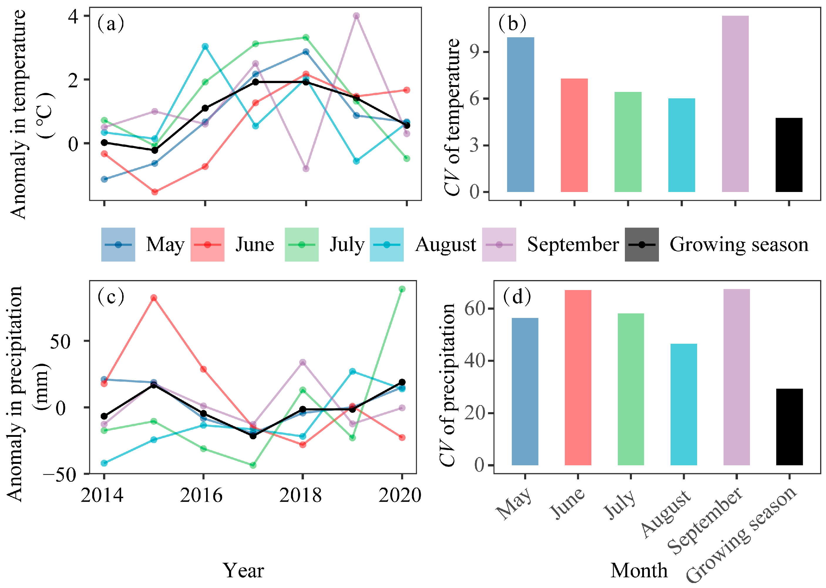
2.3.2. Climate Data
2.4. Statistical Analysis
3. Results
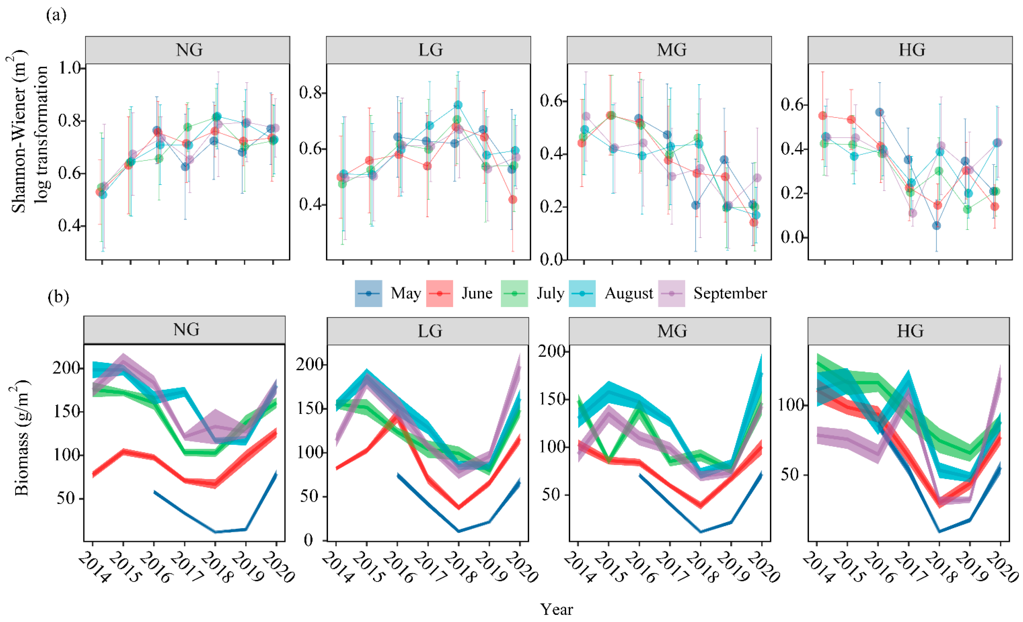
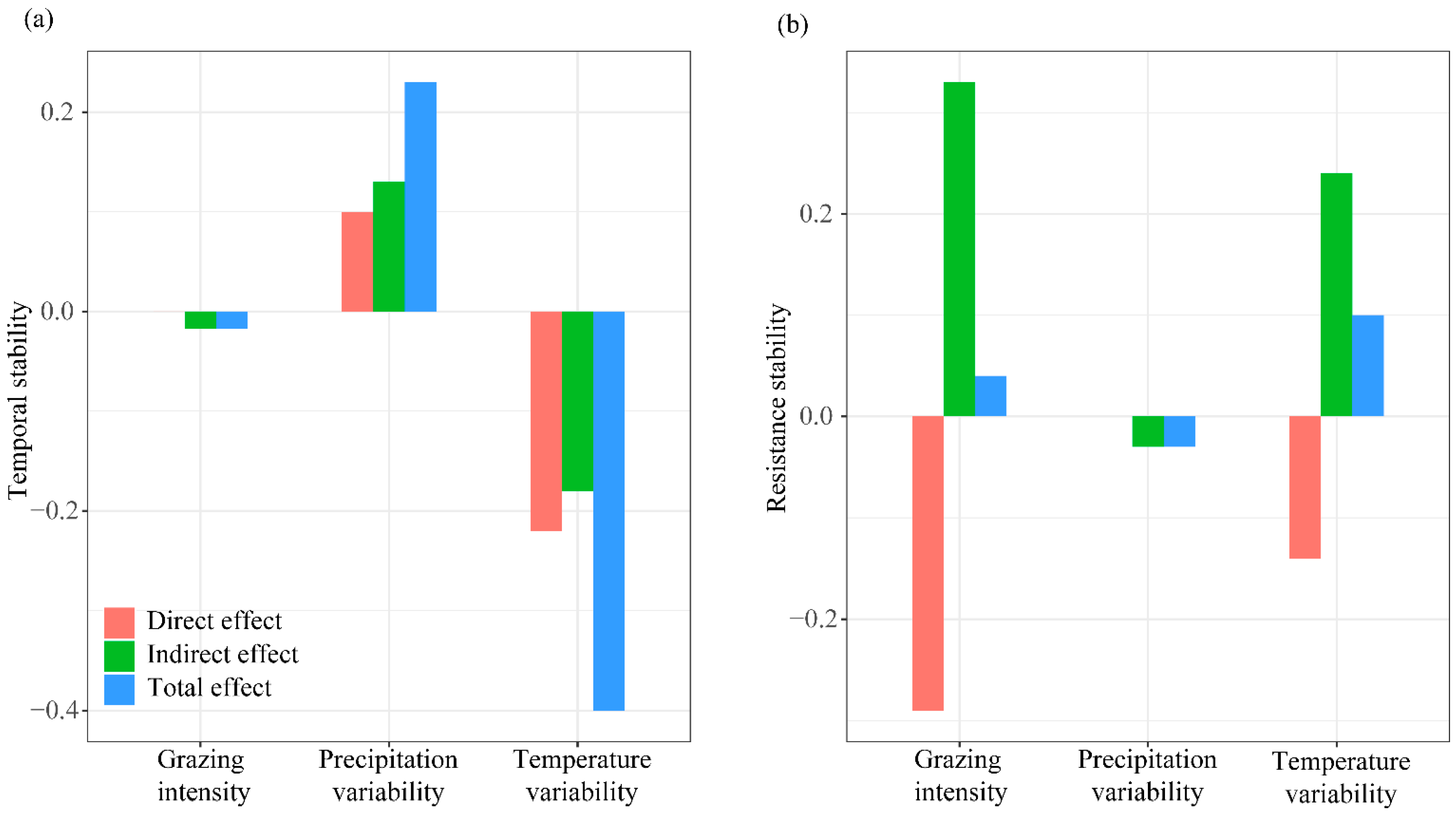
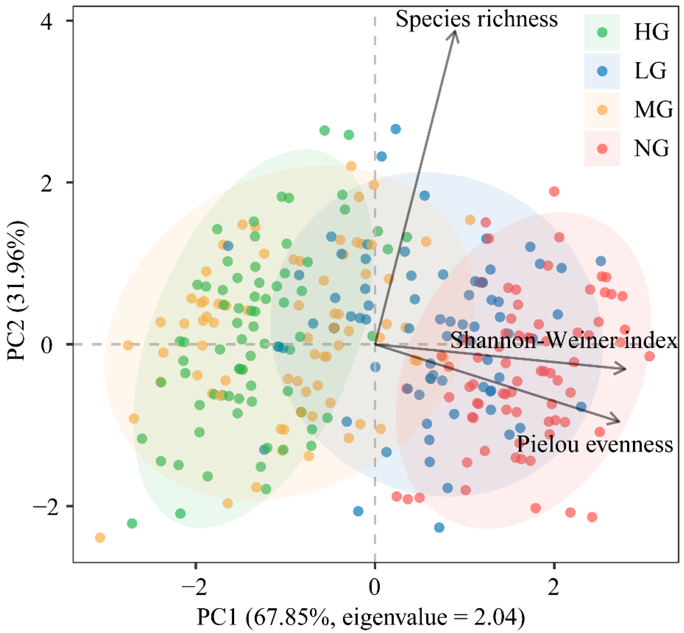
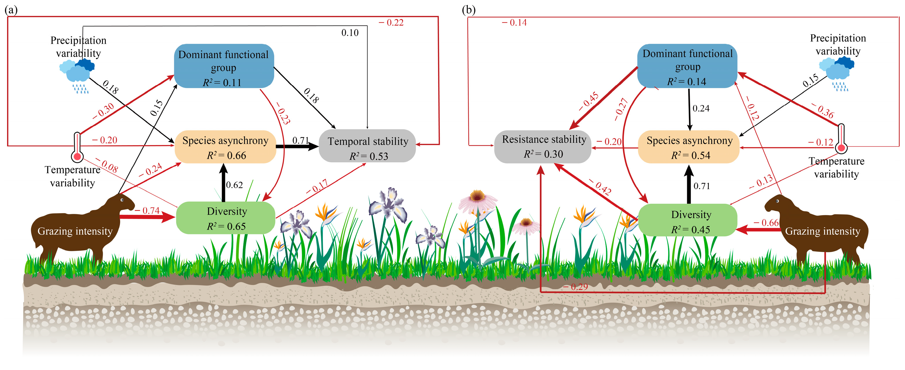
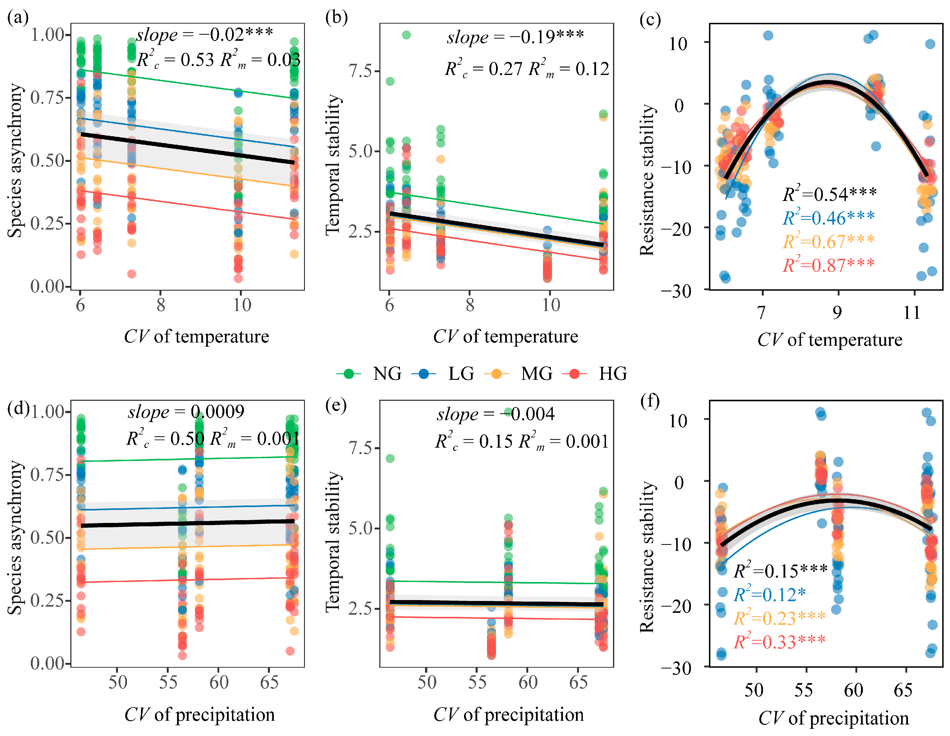
3.1. Effects of Grazing Intensity, Temperature Variability, and Precipitation Variability on Plant Community Diversity and Species Asynchrony, Temporal Stability
3.2. Effects of Grazing Intensity, Temperature Variability, and Precipitation Variability on Resistance Stability
4. Discussion
4.1. Grazing Impacts the Temporal Stability of Productivity, Not Resistance Stability
4.2. Opposing Regulatory Effects of Precipitation and Temperature Variability on Productivity Stability in Grazing Ecosystems
4.3. Mechanisms for Maintaining the Stability of Grassland Productivity under Climate Variability
5. Conclusions
Supplementary Materials
Author Contributions
Funding
Data Availability Statement
Acknowledgments
Conflicts of Interest
Appendix A

| Month | GI | Species Asynchrony | Temporal Stability | Resistance Stability |
|---|---|---|---|---|
| Mean ± Std | Mean ± Std | Mean ± Std | ||
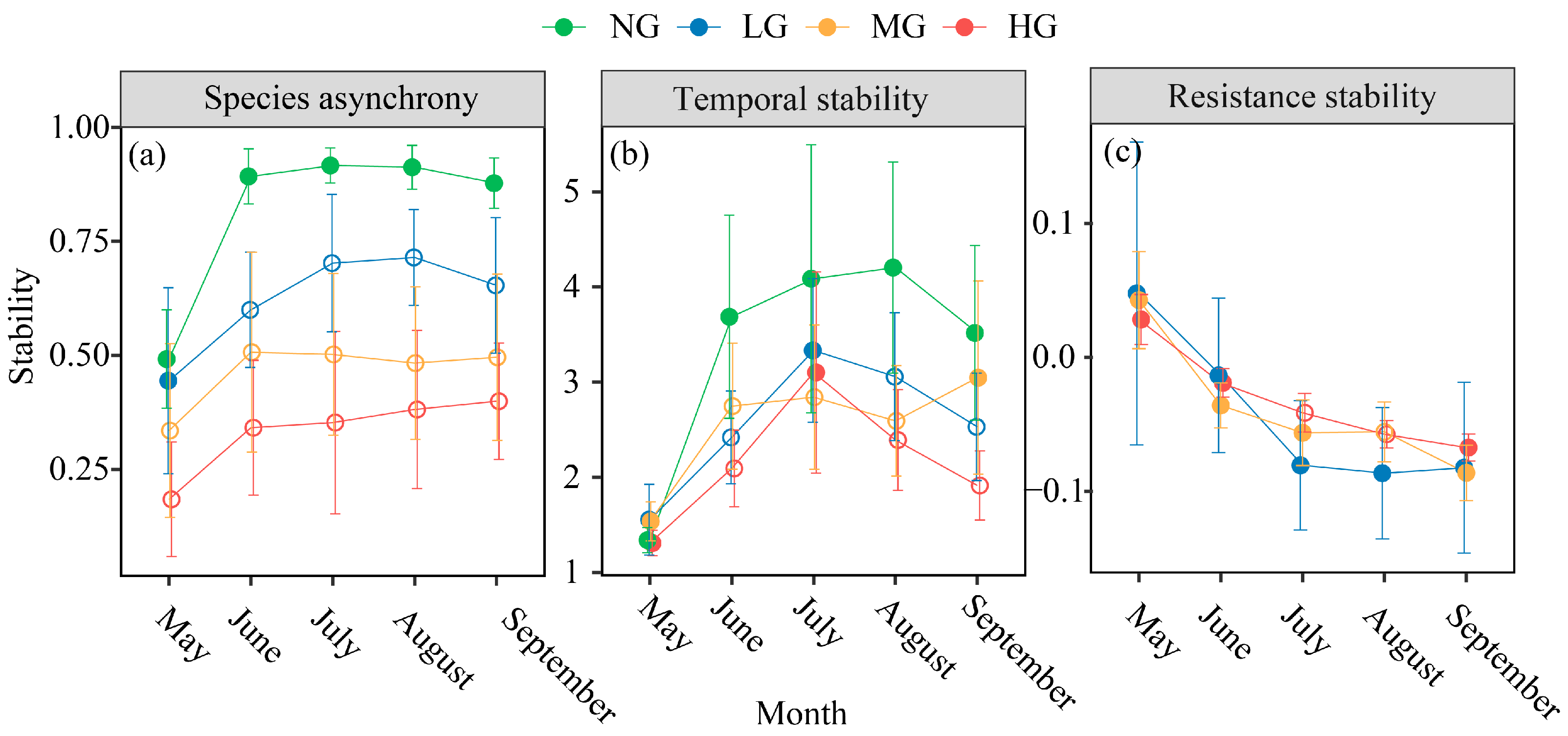
| May | HG | 0.18 ± 0.13 c | 1.31 ± 0.13 b | 0.03 ± 0.019 a |
| LG | 0.44 ± 0.20 ab | 1.56 ± 0.37 a | 0.05 ± 0.11 a | |
| MG | 0.34 ± 0.19 bc | 1.54 ± 0.20 a | 0.04 ± 0.04 a | |
| NG | 0.49 ± 0.11 a | 1.34 ± 0.13 ab | ||
| June | HG | 0.34 ± 0.15 c | 2.09 ± 0.40 b | −0.02 ± 0.01 a |
| LG | 0.60 ± 0.13 b | 2.42 ± 0.49 b | −0.01 ± 0.06 a | |
| MG | 0.51 ± 0.22 b | 2.75 ± 0.66 b | −0.04 ± 0.02 a | |
| NG | 0.89 ± 0.06 a | 3.69 ± 1.07 a | ||
| July | HG | 0.35 ± 0.20 c | 3.10 ± 1.06 ab | −0.04 ± 0.01 a |
| LG | 0.70 ± 0.15 b | 3.33 ± 0.75 ab | −0.08 ± 0.05 b | |
| MG | 0.50 ± 0.18 c | 2.84 ± 0.76 b | −0.06 ± 0.02 ab | |
| NG | 0.92 ± 0.04 a | 4.09 ± 1.41 a | ||
| August | HG | 0.39 ± 0.17 c | 2.39 ± 0.53 b | −0.06 ± 0.01 a |
| LG | 0.71 ± 0.11 b | 3.06 ± 0.67 b | −0.09 ± 0.05 b | |
| MG | 0.48 ± 0.17 c | 2.59 ± 0.58 b | −0.06 ± 0.02 a | |
| NG | 0.91 ± 0.05 a | 4.20 ± 1.11 a | ||
| September | HG | 0.40 ± 0.13 c | 1.91 ± 0.36 c | −0.07 ± 0.01 a |
| LG | 0.65 ± 0.15 b | 2.53 ± 0.56 bc | −0.08 ± 0.06 a | |
| MG | 0.50 ± 0.18 c | 3.05 ± 1.02 ab | −0.09 ± 0.02 a | |
| NG | 0.88 ± 0.06 a | 3.52 ± 0.92 a |
| Biomass | Shannon-Wiener | |||
|---|---|---|---|---|
| F | P | F | P | |
| GI | 39.15 | <0.001 | 12.37 | 0.002 |
| Y | 46.10 | <0.001 | 5.55 | 0.04 |
| M | 195.26 | <0.001 | 2.40 | 0.16 |
| GI × Y | 1.95 | 0.20 | 17.47 | <0.001 |
| GI × M | 37.51 | <0.001 | 1.79 | 0.23 |
| Y × M | 0.35 | 0.57 | 64.93 | <0.001 |
| GI × Y × M | 11.50 | 0.003 | 18.95 | <0.001 |

References
- Ives, A.R.; Carpenter, S.R. Stability and diversity of ecosystems. Science 2007, 317, 58–62. [Google Scholar] [CrossRef] [PubMed] [Green Version]
- Hautier, Y.; Tilman, D.; Isbell, F.; Seabloom, E.W.; Borer, E.T.; Reich, P.B. Anthropogenic environmental changes affect ecosystem stability via biodiversity. Science 2015, 348, 336–340. [Google Scholar] [CrossRef] [Green Version]
- Pimm, S.L. The complexity and stability of ecosystems. Nature 1984, 307, 321–326. [Google Scholar] [CrossRef]
- Donohue, I.; Hillebrand, H.; Montoya, J.M.; Petchey, O.L.; Pimm, S.L.; Fowler, M.S.; Healy, K.; Jackson, A.L.; Lurgi, M.; McClean, D.; et al. Navigating the complexity of ecological stability. Ecol. Lett. 2016, 19, 1172–1185. [Google Scholar] [CrossRef] [PubMed] [Green Version]
- Sala, O.E.; Yahdjian, L.; Havstad, K.; Aguiar, M.R. Rangeland ecosystem services: Nature’s supply and humans’ demand. In Rangeland Systems: Processes, Management and Challenges; Briske, D.D., Ed.; Springer: Berlin/Heidelberg, Germany, 2017; pp. 467–489. [Google Scholar] [CrossRef]
- Li, Z.; Ye, X.; Wang, S. Ecosystem stability and its relationship with biodiversity. Chin. J. Plant Ecol. 2021, 45, 1127–1139. [Google Scholar] [CrossRef]
- Wang, L.; Jiao, W.; MacBean, N.; Rulli, M.C.; Manzoni, S.; Vico, G.; D’odorico, P. Dryland productivity under a changing climate. Nat. Clim. Chang. 2022, 12, 981–994. [Google Scholar] [CrossRef]
- Liang, M.; Liang, C.; Hautier, Y.; Wilcox, K.R.; Wang, S. Grazing-induced biodiversity loss impairs grassland ecosystem stability at multiple scales. Ecol. Lett. 2021, 24, 2054–2064. [Google Scholar] [CrossRef]
- Ganguli, A.C.; O’Rourke, M.E. How vulnerable are rangelands to grazing? Science 2022, 378, 834. [Google Scholar] [CrossRef]
- Kéfi, S.; Domínguez-García, V.; Donohue, I.; Fontaine, C.; Thébault, E.; Dakos, V. Advancing our understanding of ecological stability. Ecol. Lett. 2019, 22, 1349–1356. [Google Scholar] [CrossRef]
- Xu, Z.; Liu, H.; Meng, Y.; Yin, J.; Ren, H.; Li, M.-H.; Yang, S.; Tang, S.; Jiang, Y.; Jiang, L. Nitrogen addition and mowing alter drought resistance and recovery of grassland communities. Sci. China Life Sci. 2023, 66, 1682–1692. [Google Scholar] [CrossRef]
- Ganjurjav, H.; Zhang, Y.; Gornish, E.S.; Hu, G.; Li, Y.; Wan, Y.; Gao, Q. Differential resistance and resilience of functional groups to livestock grazing maintain ecosystem stability in an alpine steppe on the Qinghai-Tibetan Plateau. J. Environ. Manag. 2019, 251, 109579. [Google Scholar] [CrossRef]
- Pennekamp, F.; Pontarp, M.; Tabi, A.; Altermatt, F.; Alther, R.; Choffat, Y.; Fronhofer, E.A.; Ganesanandamoorthy, P.; Garnier, A.; Griffiths, J.I.; et al. Biodiversity increases and decreases ecosystem stability. Nature 2018, 563, 109–112. [Google Scholar] [CrossRef] [Green Version]
- McCann, K.S. The diversity-stability debate. Nature 2000, 405, 228–233. [Google Scholar] [CrossRef]
- Loreau, M.; de Mazancourt, C. Biodiversity and ecosystem stability: A synthesis of underlying mechanisms. Ecol. Lett. 2013, 16, 106–115. [Google Scholar] [CrossRef]
- Isbell, F.I.; Polley, H.W.; Wilsey, B.J. Biodiversity, productivity and the temporal stability of productivity: Patterns and processes. Ecol. Lett. 2009, 12, 443–451. [Google Scholar] [CrossRef] [Green Version]
- Wright, A.J.; Ebeling, A.; de Kroon, H.; Roscher, C.; Weigelt, A.; Buchmann, N.; Buchmann, T.; Fischer, C.; Hacker, N.; Hildebrandt, A.; et al. Flooding disturbances increase resource availability and productivity but reduce stability in diverse plant communities. Nat. Commun. 2015, 6, 6092. [Google Scholar] [CrossRef] [Green Version]
- Cardinale, B.J.; Duffy, J.E.; Gonzalez, A.; Hooper, D.U.; Perrings, C.; Venail, P.; Narwani, A.; Mace, G.M.; Tilman, D.; Wardle, D.A.; et al. Biodiversity loss and its impact on humanity. Nature 2012, 486, 59–67. [Google Scholar] [CrossRef] [Green Version]
- Hillebrand, H.; Langenheder, S.; Lebret, K.; Lindström, E.; Östman, Ö.; Striebel, M. Decomposing multiple dimensions of stability in global change experiments. Ecol. Lett. 2018, 21, 21–30. [Google Scholar] [CrossRef] [Green Version]
- Donohue, I.; Petchey, O.L.; Montoya, J.M.; Jackson, A.L.; McNally, L.; Viana, M.; Healy, K.; Lurgi, M.; O’Connor, N.E.; Emmerson, M.C.; et al. On the dimensionality of ecological stability. Ecol. Lett. 2013, 16, 421–429. [Google Scholar] [CrossRef]
- MacDougall, A.S.; McCann, K.S.; Gellner, G.; Turkington, R. Diversity loss with persistent human disturbance increases vulnerability to ecosystem collapse. Nature 2013, 494, 86–89. [Google Scholar] [CrossRef]
- Koerner, S.E.; Smith, M.D.; Burkepile, D.E.; Hanan, N.P.; Avolio, M.L.; Collins, S.L.; Knapp, A.K.; Lemoine, N.P.; Forrestel, E.J.; Eby, S.; et al. Change in dominance determines herbivore effects on plant biodiversity. Nat. Ecol. Evol. 2018, 2, 1925–1932. [Google Scholar] [CrossRef]
- Beck, J.J.; Hernández, D.L.; Pasari, J.R.; Zavaleta, E.S. Grazing maintains native plant diversity and promotes community stability in an annual grassland. Ecol. Appl. 2015, 25, 1259–1270. [Google Scholar] [CrossRef] [Green Version]
- Mortensen, B.; Danielson, B.; Harpole, W.S.; Alberti, J.; Arnillas, C.A.; Biederman, L.; Borer, E.T.; Cadotte, M.W.; Dwyer, J.M.; Hagenah, N.; et al. Herbivores safeguard plant diversity by reducing variability in dominance. J. Ecol. 2017, 106, 101–112. [Google Scholar] [CrossRef] [Green Version]
- Zhang, Y.; Loreau, M.; He, N.; Wang, J.; Pan, Q.; Bai, Y.; Han, X. Climate variability decreases species richness and community stability in a temperate grassland. Oecologia 2018, 188, 183–192. [Google Scholar] [CrossRef]
- Gherardi, L.A.; Sala, O.E. Effect of interannual precipitation variability on dryland productivity: A global synthesis. Glob. Chang. Biol. 2019, 25, 269–276. [Google Scholar] [CrossRef] [Green Version]
- Knapp, A.K.; Ciais, P.; Smith, M.D. Reconciling inconsistencies in precipitation-productivity relationships: Implications for climate change. New Phytol. 2017, 214, 41–47. [Google Scholar] [CrossRef] [Green Version]
- Ma, Z.; Liu, H.; Mi, Z.; Zhang, Z.; Wang, Y.; Xu, W.; Jiang, L.; He, J.-S. Climate warming reduces the temporal stability of plant community biomass production. Nat. Commun. 2017, 8, 15378. [Google Scholar] [CrossRef] [Green Version]
- Yan, Y.; Connolly, J.; Liang, M.; Jiang, L.; Wang, S. Mechanistic links between biodiversity effects on ecosystem functioning and stability in a multi-site grassland experiment. J. Ecol. 2021, 109, 3370–3378. [Google Scholar] [CrossRef]
- Tilman, D. The Ecological Consequences of Changes in Biodiversity: A Search for General Principles101. Ecology 1999, 80, 1455–1474. [Google Scholar] [CrossRef] [Green Version]
- Li, W.; Li, X.; Zhao, Y.; Zheng, S.; Bai, Y. Ecosystem structure, functioning and stability under climate change and grazing in grasslands: Current status and future prospects. Curr. Opin. Environ. Sustain. 2018, 33, 124–135. [Google Scholar] [CrossRef]
- Hallett, L.M.; Stein, C.; Suding, K.N. Functional diversity increases ecological stability in a grazed grassland. Oecologia 2017, 183, 831–840. [Google Scholar] [CrossRef]
- Blüthgen, N.; Simons, N.K.; Jung, K.; Prati, D.; Renner, S.C.; Boch, S.; Fischer, M.; Hölzel, N.; Klaus, V.H.; Kleinebecker, T.; et al. Land use imperils plant and animal community stability through changes in asynchrony rather than diversity. Nat. Commun. 2016, 7, 10697. [Google Scholar] [CrossRef] [Green Version]
- Qin, J.; Ren, H.; Han, G.; Zhang, J.; Browning, D.; Willms, W.; Yang, D. Grazing reduces the temporal stability of temperate grasslands in northern China. Flora 2019, 259, 151450. [Google Scholar] [CrossRef]
- Wu, Y.; Guo, Z.; Li, Z.; Liang, M.; Tang, Y.; Zhang, J.; Miao, B.; Wang, L.; Liang, C. The main driver of soil organic carbon differs greatly between topsoil and subsoil in a grazing steppe. Ecol. Evol. 2022, 12, e9182. [Google Scholar] [CrossRef]
- Shannon, C.E. A Mathematical Theory of Communication. Bell Syst. Tech. J. 1948, 27, 379–423. [Google Scholar] [CrossRef] [Green Version]
- Pielou, E.C. The measurement of diversity in different types of biological collections. J. Theor. Biol. 1967, 15, 177. [Google Scholar] [CrossRef]
- Loreau, M.; de Mazancourt, C. Species synchrony and its drivers: Neutral and nonneutral community dynamics in fluctuating environments. Am. Nat. 2008, 172, E48–E66. [Google Scholar] [CrossRef] [Green Version]
- Lehman, C.L.; Tilman, D. Biodiversity, Stability, and Productivity in Competitive Communities. Am. Nat. 2000, 156, 534–552. [Google Scholar] [CrossRef]
- Dominguez-Garcia, V.; Dakos, V.; Kefi, S. Unveiling dimensions of stability in complex ecological networks. Proc. Natl. Acad. Sci. USA 2019, 116, 25714–25720. [Google Scholar] [CrossRef]
- Lefcheck, J.S.; Freckleton, R. piecewiseSEM: Piecewise structural equation modelling in r for ecology, evolution, and systematics. Methods Ecol. Evol. 2015, 7, 573–579. [Google Scholar] [CrossRef]
- Milchunas, D.G.; Lauenroth, W.K. Quantitative Effects of Grazing on Vegetation and Soils Over a Global Range of Environments. Ecol. Monogr. 1993, 63, 327–366. [Google Scholar] [CrossRef]
- He, F.; Yang, J.; Dong, S.; Zhi, Y.; Hao, X.; Shen, H.; Xiao, J.; Kwaku, E.A.; Zhang, R.; Shi, H.; et al. Short-term grazing changed temporal productivity stability of alpine grassland on Qinghai-Tibetan Plateau via response species richness and functional groups asynchrony. Ecol. Indic. 2023, 146, 109800. [Google Scholar] [CrossRef]
- Chen, Q.; Wang, S.; Seabloom, E.W.; MacDougall, A.S.; Borer, E.T.; Bakker, J.D.; Donohue, I.; Knops, J.M.H.; Morgan, J.W.; Carroll, O.; et al. Nutrients and herbivores impact grassland stability across spatial scales through different pathways. Glob. Chang. Biol. 2022, 28, 2678–2688. [Google Scholar] [CrossRef] [PubMed]
- Wang, S.; Isbell, F.; Deng, W.; Hong, P.; Dee, L.E.; Thompson, P.; Loreau, M. How complementarity and selection affect the relationship between ecosystem functioning and stability. Ecology 2021, 102, e03347. [Google Scholar] [CrossRef]
- Le Bagousse-Pinguet, Y.; Gross, E.M.; Straile, D. Release from competition and protection determine the outcome of plant interactions along a grazing gradient. Oikos 2012, 121, 95–101. [Google Scholar] [CrossRef]
- Oñatibia, G.R.; Boyero, L.; Aguiar, M.R. Regional productivity mediates the effects of grazing disturbance on plant cover and patch-size distribution in arid and semi-arid communities. Oikos 2018, 127, 1205–1215. [Google Scholar] [CrossRef]
- Harrison, S.; LaForgia, M. Seedling traits predict drought-induced mortality linked to diversity loss. Proc. Natl. Acad. Sci. USA 2019, 116, 5576–5581. [Google Scholar] [CrossRef] [Green Version]
- Ma, F.; Zhang, F.; Quan, Q.; Song, B.; Wang, J.; Zhou, Q.; Niu, S. Common Species Stability and Species Asynchrony Rather than Richness Determine Ecosystem Stability Under Nitrogen Enrichment. Ecosystems 2020, 24, 686–698. [Google Scholar] [CrossRef]
- Muraina, T.O.; Xu, C.; Yu, Q.; Yang, Y.; Jing, M.; Jia, X.; Jaman, S.; Dam, Q.; Knapp, A.K.; Collins, S.L.; et al. Species asynchrony stabilises productivity under extreme drought across Northern China grasslands. J. Ecol. 2021, 109, 1665–1675. [Google Scholar] [CrossRef]
- Abrams, P.A.; Tucker, C.M.; Gilbert, B. Evolution of the storage effect. Evolution 2013, 67, 315–327. [Google Scholar] [CrossRef]
- Shurin, J.B.; Winder, M.; Adrian, R.; Keller, W.; Matthews, B.; Paterson, A.M.; Paterson, M.J.; Pinel-Alloul, B.; Rusak, J.A.; Yan, N.D. Environmental stability and lake zooplankton diversity—Contrasting effects of chemical and thermal variability. Ecol. Lett. 2010, 13, 453–463. [Google Scholar] [CrossRef]
- Tilman, D.; Downing, J.A. Biodiversity and stability in grasslands. Nature 1994, 367, 363–365. [Google Scholar] [CrossRef]
- Tilman, D. Biodiversity: Population Versus Ecosystem Stability. Ecology 1995, 77, 350–363. [Google Scholar] [CrossRef]
- Pfisterer, A.B.; Schmid, B. Diversity-dependent production can decrease the stability of ecosystem functioning. Nature 2002, 416, 84–86. [Google Scholar] [CrossRef]

| GI | M | GI × M | ||||
|---|---|---|---|---|---|---|
| F | p | F | p | F | p | |
| Species asynchrony | 20.87 | <0.001 | 0.40 | 0.54 | 0.60 | 0.63 |
| Temporal stability | 13.19 | 0.002 | 0.15 | 0.71 | 0.42 | 0.74 |
| Resistance stability | 0.49 | 0.64 | 69.08 | 0.001 | 0.83 | 0.48 |
Disclaimer/Publisher’s Note: The statements, opinions and data contained in all publications are solely those of the individual author(s) and contributor(s) and not of MDPI and/or the editor(s). MDPI and/or the editor(s) disclaim responsibility for any injury to people or property resulting from any ideas, methods, instructions or products referred to in the content. |
© 2023 by the authors. Licensee MDPI, Basel, Switzerland. This article is an open access article distributed under the terms and conditions of the Creative Commons Attribution (CC BY) license (https://creativecommons.org/licenses/by/4.0/).
Share and Cite
Han, Y.; Wu, Y.; Cui, J.; Li, H.; Li, H.; Zhang, J.; Miao, B.; Wang, L.; Li, Z.; Liang, C. Temporal Stability of Grazed Grassland Ecosystems Alters Response to Climate Variability, While Resistance Stability Remains Unchanged. Agronomy 2023, 13, 2030. https://doi.org/10.3390/agronomy13082030
Han Y, Wu Y, Cui J, Li H, Li H, Zhang J, Miao B, Wang L, Li Z, Liang C. Temporal Stability of Grazed Grassland Ecosystems Alters Response to Climate Variability, While Resistance Stability Remains Unchanged. Agronomy. 2023; 13(8):2030. https://doi.org/10.3390/agronomy13082030
Chicago/Turabian StyleHan, Ying, Yantao Wu, Jiahe Cui, Hangyu Li, Hao Li, Jinghui Zhang, Bailing Miao, Lixin Wang, Zhiyong Li, and Cunzhu Liang. 2023. "Temporal Stability of Grazed Grassland Ecosystems Alters Response to Climate Variability, While Resistance Stability Remains Unchanged" Agronomy 13, no. 8: 2030. https://doi.org/10.3390/agronomy13082030