Sensitivity Analysis of the WOFOST Crop Model Parameters Using the EFAST Method and Verification of Its Adaptability in the Yellow River Irrigation Area, Northwest China

Abstract

Sensitivity analysis, calibration, and verification of crop model parameters improve crop model efficiency and accuracy, facilitating its application. This study selected five sites within the Ningxia Yellow River Irrigation Area. Using meteorological data, soil data, and field management information, the EFAST (Extended Fourier Amplitude Sensitivity Test) method was used to conduct first-order and global sensitivity analyses of spring wheat parameters in the WOFOST (World Food Studies Simulation) Model. A Structural Equation Model (SEM) analyzed the contribution of crop parameters to different simulation indices, with parameter sensitivity rankings being discussed under varying water supply and climate conditions. Finally, the adapted WOFOST model was employed to assess its applicability in the Ningxia Yellow River Irrigation Area. TMNFTB3.0 (correction factor of total assimilation rate at 3 °C), SPAN (life span of leaves growing at 35 °C), SLATB0 (specific leaf area in the initial period), and CFET (correction factor transpiration rate) showed higher sensitivity index for most simulation indices. Under the same meteorological conditions, different water supply conditions have a limited impact on crop parameter sensitivity, mainly affecting leaf senescence, leaf area, and assimilate conversion to storage organs. The corrected crop parameters significantly enhanced the wheat yield simulation accuracy by the WOFOST model ($M_E$ = 0.9964; $R_{MSE}$ = 0.2516; $M_{BE}$ = 0.1392; $R^2$ = 0.0331). The localized WOFOST model can predict regional crop yield, with this study providing a theoretical foundation for its regional application, adjustment, and optimization.

1. Introduction

In recent years, global climate change has significantly affected wheat production due to changes in climate factors [1]. Thus, accurate and rapid simulation of wheat growth, development, and yield changes under different conditions is crucial for guiding wheat production [2]. Currently, crop growth models are extensively utilized in predicting crop yield [3], managing agriculture [4], and evaluating agricultural production potential [5] and other related fields. Existing crop models (WOFOST, CERES, APSIM, etc., the full name of models is shown in Appendix A, Table A2) are widely employed for monitoring and evaluating the growth and yield of crops like wheat, rice, corn, soybean and others [6,7,8,9], due to their strong logic and practicality. However, with time, as agriculture faces increasing challenges, these models show higher complexity [10]. They mathematically represent the intricate interplay among plants, weather, soil, and field management, requiring significant human and financial resources for parameter acquisition for model utilization [11]. Parameter estimation is crucial in model development, as it determines prediction accuracy [12]. However, focusing on sensitive parameters can enhance model calibration accuracy and efficiency, as crop growth models often involve multiple parameters with significant impact under certain scenarios [13]. Sensitivity analysis (SA) is a widely utilized tool for calibrating and developing crop growth models, enabling quantification of parameter impacts on model output [14].

SA can allocate uncertain outcomes to various model parameters, quantify their impact on output results, and identify and select crucial model parameters, thereby reducing the workload in parameter optimization while minimizing output uncertainty [15]. SA finds wide application in various crop models, including DSSAT [16], WOFOST [17], APSIM [18] and others. It can be divided into first-order SA and global SA [19]. The former estimates the impact of a single parameter on model output while keeping other parameters fixed, and it is commonly used due to its efficiency and speed [20]. Global SA considers and quantitatively represents the impact of individual parameters and their interactions [21]. Commonly used SA methods in crop model studies include EFAST [22], Morris [23], Fourier Amplitude Sensitivity Test (FAST) [24], Sobol [25], and others [26,27]. Among them, the Extended Fourier Amplitude Sensitivity Test (EFAST) method based on variance analysis combines the advantages of FAST and Sobol methods. It calculates parameter interactions and provides efficient and accurate results [28]. Previous studies have successfully employed EFAST for crop growth model SA [29,30,31] and generated promising outcomes. However, most existing SA studies focus on yield and above-ground biomass at maturity as observational variables [32], neglecting other constantly changing variables like leaf area index (LAI). SA can assess the impact of minor variations in parameter values on model outcomes [33] or globally evaluate the interaction of the entire range of parameter values [34]. The latter approach typically involves difference analysis using the Taylor series and Monte Carlo methods [35].

Therefore, conducting SA, calibration, and validation of crop model parameters enhance and optimize the model’s efficiency, accuracy, and applicability. In this study, the Yellow River irrigation area of Ningxia Hui Autonomous Region served as the research site. Field measurements, statistical survey data on spring wheat, and local meteorological, soil, and field management test data were utilized for an EFAST SA in the WOFOST model. This analysis examined the impact of crop parameters on spring wheat growth and yield simulation results. Parameter sensitivity and their ranking consistency were discussed under varying water supply conditions and climate scenarios, with underlying causes being explored for sensitivity differences. Finally, the optimized model’s adaptability was verified in the Ningxia Yellow River Irrigation Area, providing technical support for parameter SA to help localize the WOFOST model. Given the significant reference value of the WOFOST model in wheat production, this study proposes a comprehensive approach to determine model parameters by integrating actual wheat yield data. It presents sensitivity variations of different parameters under diverse conditions, aiming to offer practical insights for the application of the WOFOST model. Additionally, it offered effective methods for crop model parameter calibration and application, and established a foundation for future regional-scale model parameter calibration and verification.

2. Materials and Methods

2.1. Overview and Data Sources of the Study Area

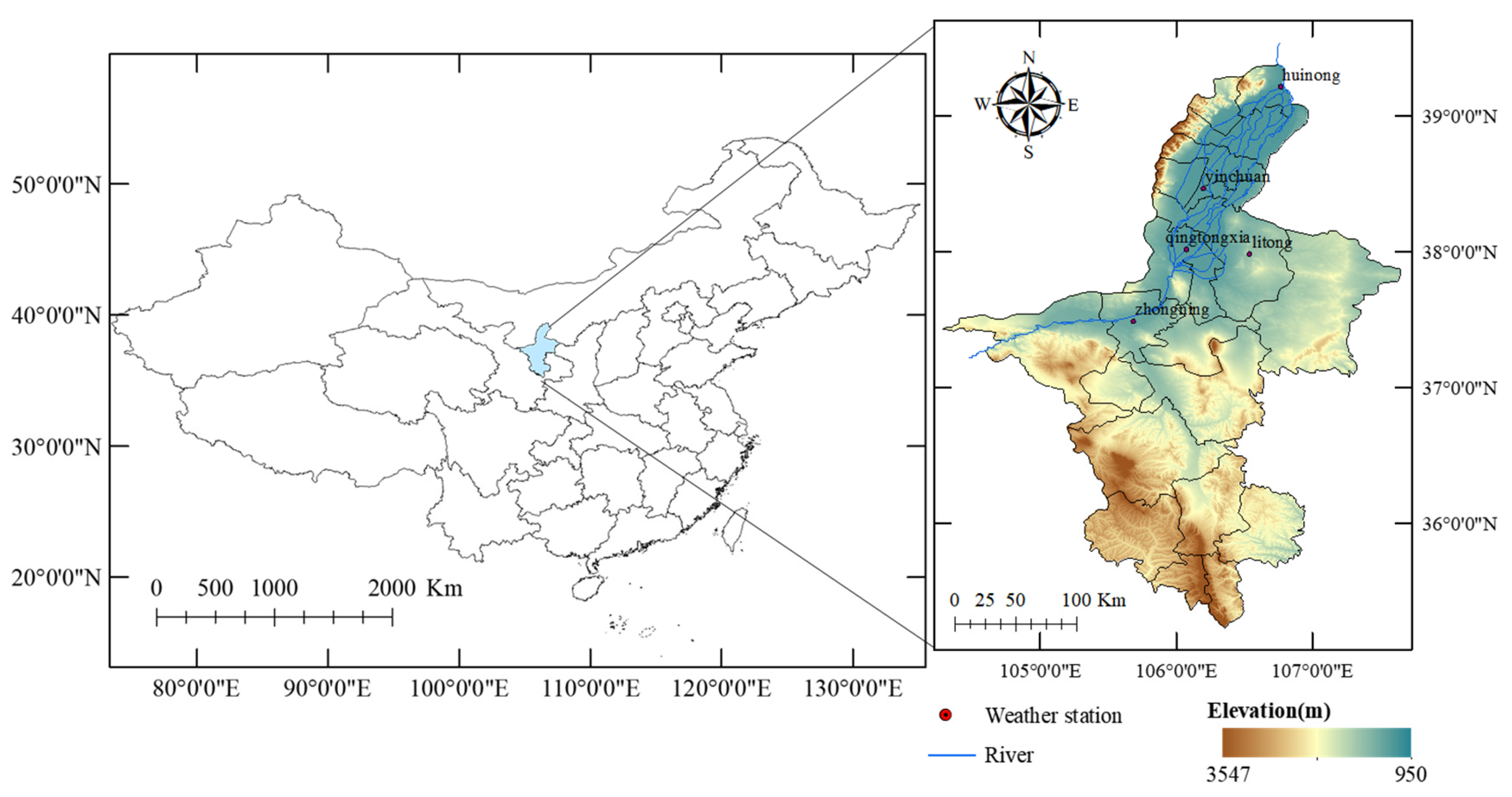
Ningxia, situated in northwest China, is located between 35°14′–39°23′ N and 104°17′–107°39′ E, in the upper reaches of the Yellow River. The area covers a total landmass of ~66,400 km² (Figure 1). This study selected five agro-meteorological testing stations in Huinong, Yinchuan, Litong, Zhongning, and Qingtongxia as research areas due to their significance as primary planting regions for spring wheat. Meteorological data used in this study were sourced from the National Data Center for Meteorological Sciences (http://data.cma.cn), while the fundamental soil data for the model operation were obtained through field measurements and the China Soil Database (http://vdb3.soil.csdb.cn, China). These details are presented in Table 1.

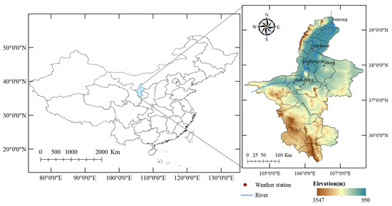
Figure 1. Scope of the study area and distribution of meteorological stations.

Table 1. Information on the latitude, longitude, and fundamental physical and chemical soil properties at the experimental site.

Research Area	Organic Carbon Content/(g·kg−1)	Crushed Stone Volume/%	Sand Content/%	Silt Content/%	Clay Content/%	Soil Bulk Density/g·cm−3	PH Value
Yinchuan	1.12	10	29	50	21	1.38	7.8
Litong	0.46	7	41	38	21	1.4	8.1
Zhongning	1.12	10	34	45	21	1.39	7.9
Huinong	0.46	7	41	38	21	1.4	8.1
Qingtongxia	1.12	10	29	50	21	1.38	7.8

2.2. WOFOST Model

The WOFOST model, collaboratively developed by the Wageningen University and the World Food Research Center (CWFS) in the Netherlands, is a versatile model with diverse crop parameters applicable to various crops. Its calculation process is primarily executed through three modules: climate, crop, and soil. By utilizing daily meteorological data, the model establishes dynamic explanatory models for crop growth based on soil conditions, management practices, and crop parameters [36]. These models simulate crop growth under three conditions: potential, water-limited, and nutrient-limited [37]. The WOFOST model incorporates major biophysical and biochemical processes. The three developmental stages of crops (DVS) are represented by dimensionless variables: DVS 0 (represents the seedling stage), DVS 1 (represents the flowering stage), and DVS 2 (represents the maturity stage) [38].

For model operation, the following soil parameters are necessary: (1) soil moisture content at wilting point (SWM; cm³/cm³), soil moisture content at field capacity (SMFCF; cm³/cm³), soil moisture content at saturation (SM0; cm³/cm³), and hydraulic conductivity of saturated soil (K0; cm/day). These were determined using the Van Genuchten (VG) model [39], with VG parameters derived from the Rosetta model [40] based on the soil’s fundamental physicochemical properties. The Mualem model [41] was also employed to obtain the soil water conductivity function, calculated via Python program and converted into the requisite soil parameters. The VG model is shown in Equation (1).

$$\mathsf{\Theta }=\frac{\theta -{\theta }_r}{{\theta }_s-{\theta }_r}={\left[\frac{1}{1+{\left(\alpha h\right)}^n}\right]}^m$$

(1)

where $\mathsf{\Theta }$ is the effective soil water content at a given soil suction of h (kPa) (cm³/cm³); ${\theta }_s$ is saturation moisture content (cm³/cm³); ${\theta }_r$ is the retained water content (cm³/cm³); $\alpha$ is scale parameter (1/kPa); and m and n are shape parameter. The meteorological parameters necessary for model operation are computed using the Food and Agriculture Organization of the United Nations (FAO)-recommended Penman-Monteith formula, as shown below:

$$R_a=\frac{24\left(60\right)}{\pi }{G}_{sc}{d}_r\left[{\omega }_s\sin \left(\phi \right)\sin \left(\delta \right)+\cos \left(\phi \right)\cos \left(\delta \right)\sin \left({\omega }_s\right)\right]$$

(2)

$$d_r=1+0.033\cos \left(\frac{2\pi }{365}J\right)$$

(3)

$$\delta =0.409\sin \left(\frac{2\pi }{365}J-1.39\right)$$

(4)

where $R_a$ is the daily solar zenith radiation (MJ·m⁻²·day⁻¹); $G_{sc}$ = 0.0820 is the solar constant (MJ·m⁻²·min⁻¹); $d_r$ is the reciprocal of the relative distance between the sun and the earth; ${\omega }_s$ is the solar hour angle (rad); $\phi$ is the geographical latitude (rad); $\delta$ is the solar magnetic declination angle (rad); $J$ is the ordinal number of a day. Solar radiation ($R_s$) and steam pressure ($e_s$) can be obtained from the following equation:

$$R_s=\left(a_s+b_s\frac{n}{N}\right)R_a$$

(5)

$$e^O\left(T\right)=0.6108\exp \left[\frac{17.27T}{T+237.3}\right]$$

(6)

$$e_s=\frac{e^O\left(T_{\max }\right)+e^O\left(T_{\min }\right)}{2}$$

(7)

where $n/N$ is the relative sunshine duration; $a_s$ and $b_s$ are the regression constants; $e^O\left(T\right)$ is the water vapor pressure (kPa) at the air temperature T; $\exp \left[\dots \right]$ is an exponential function with base 2.7183. The daily average saturated water vapor pressure should be computed as the mean of the daily average maximum and minimum temperatures over that period.

2.3. Structural Equation Model

Structural Equation Model (SEM) is a multivariate statistical technique used to identify, estimate, and validate various causal models [42]. SEM is typically applied to observe multiple factor variables and generate corresponding observations [43]. It also represents the causal process in a study through a series of structural equations, which are then statistically tested to determine their consistency with empirical data across the entire variable system.

Therefore, considering the potential for multiple causal relationships between simulation indicators and crop parameter factors, employing SEM offers advantages in modeling the crop growth system [44]. In this study, SEM was utilized to examine the contribution of different crop parameters to various model indicators.

2.4. Research Methods

2.4.1. Crop Model Parameter Selection Method in WOFOST Model

Based on the growth and development characteristics of spring wheat and previous studies on crop parameters of the WOFOST model for wheat [45,46,47], a total of 39 parameters related to different growth and development stages were selected for SA. These parameters include assimilation, assimilate conversion, light energy utilization, extinction coefficient, leaf development, evapotranspiration, dry matter allocation, root system, and water use. SA was conducted by varying the model crop parameters within ±10% of their default values and the default parameter range, assuming an even distribution within this range (Table 2).

Table 2. Unit and value range of crop parameters in the WOFOST model.

Parameter	Significance	Unit	Lower Limiting Value	Upper Limiting Value	Parameter	Significance	Unit	Lower Limiting Value	Upper Limiting Value
AMAXTB0	Maximum CO2 assimilation rate under DVS = 0	kg·hm−2·h−1	32.247	39.413	TMPFTB35	Correction factor of maximum assimilation rate under mean temperature 25 °C		0	0.1
AMAXTB1.0	Maximum CO2 assimilation rate under DVS = 1.0	kg·hm−2·h−1	32.247	39.413	TBASE	Lower threshold temperature for emergence		−2	2
AMAXTB1.3	Maximum CO2 assimilation rate under DVS = 1.3	kg·hm−2·h−1	32.247	39.413	TSUM1	Cumulative Temperature from emergence to flowering	°C·d	800	1500
AMAXTB2.0	Maximum CO2 assimilation rate under DVS = 2.0	kg·hm−2·h−1	4.032	4.928	TSUM2	Cumulative Temperature from flowering to maturity	°C·d	600	1350
CVO	Efficiency of conversion into storage organs	kg·kg−1	0.6381	0.7799	TMNFTB0	Correction factor of total assimilation rate under minimum temperature 0 °C		0	0.1
CVL	Efficiency of conversion into leaves	kg·kg−1	0.6165	0.7535	TMNFTB30	Correction factor of total assimilation rate under minimum temperature 0 °C		0.9	1.1
CVS	Efficiency of conversion into stems	kg·kg−1	0.63	0.7282	LAIEM	Leaf area index at emergence	hm2·hm−2	0.12285	0.15015
CVR	Efficiency of conversion into roots	kg·kg−1	0.65	0.7634	FOTB1	The dry matter distribution coefficient of storage organs increased under DVS = 1	kg·kg−1	0.9	1.1
EFFTB0	Light energy utilization rate of single leaf under average daily temperature 0 °C	kg·hm−2·h−1·J−1·m2·s	0.405	0.495	CFET	Correction factor transpiration rate		0.9	1.1
EFFTB40	Light energy utilization rate of single leaf under average daily temperature 40 °C	kg·hm−2·h−1·J−1·m2·s	0.405	0.495	FLTB0	Leaf dry matter distribution coefficient under DVS = 0	kg·kg−1	0.585	0.715
KDIFTB0	Extinction coefficient for diffuse visible light under DVS = 0		0.54	0.66	FLTB0.25	Leaf dry matter distribution coefficient under DVS = 0.25	kg·kg−1	0.63	0.77
KDIFTB2.0	Extinction coefficient for diffuse visible light under DVS = 2.0		0.54	0.66	FLTB0.5	Leaf dry matter distribution coefficient under DVS = 0.5	kg·kg−1	0.45	0.55
SPAN	Life span of leaves growing at 35 Celsius	d	28.17	34.43	FLTB0.646	Leaf dry matter distribution coefficient under DVS = 0.646	kg·kg−1	0.27	0.33
SLATB0	Specific leaf area under DVS = 0	hm2·kg−1	0.001908	0.002332	DEPNR	Crop group number for soil water depletion		4.05	4.95
SLATB0.5	Specific leaf area under DVS = 0.5	hm2·kg−1	0.001908	0.002332	TDWI	Initial total crop dry weight	kg·hm−2	180	220
SLATB2.0	Specific leaf area under DVS = 2.0	hm2·kg−1	0.001908	0.002332	Q10	Relative change in respiratory rate for every 10 °C temperature change		1.8	2
TMPFTB0	Correction factor of maximum assimilation rate under mean temperature 0 °C		0.009	0.1	RDI	Initial rooting depth	cm	10	12
TMPFTB10	Correction factor of maximum assimilation rate under mean temperature 0 °C		0.54	1	RRI	Maximum daily increase in rooting depth	cm·d−1	1.08	1.32
TMPFTB15	Correction factor of maximum assimilation rate under mean temperature 15 °C		0.9	1	RDMCR	Maximum rooting depth	cm	112.5	137.5
TMPFTB25	Correction factor of maximum assimilation rate under mean temperature 25 °C		0.9	1

2.4.2. EFAST Analysis Method

To analyze the contribution of crop input parameters to output variables and address high-order interactions, the EFAST method was used, which is a globally applicable and quantitative algorithm that effectively handles complex non-linear and non-monotonic models [48,49]. This method provides first-order and global sensitivity indices for each parameter [50]. EFAST combines the computational efficiency of the FAST algorithm and the ability to calculate the total effects of the Sobol algorithm [51]. It has recently gained popularity in hydrological, ecological, and meteorological modeling due to its inherent advantages [52,53,54,55].

The EFAST algorithm comprises two main steps: sampling and sensitivity index calculation [56]. First, an efficient and uniform sampling process is performed using a transform function. Then, FAST was used to obtain a quantitative sensitivity index, which establishes the total variance of the model determined by each parameter and their interactions. Finally, the total variance of the model is decomposed into its constituent parts:

$$V\left(Y\right)={\displaystyle \sum _{i=1}^n{V}_i+{\displaystyle \sum _{i<j\le n}^n{V}_{ij}+\cdots +V_{\left(1,2,\cdots ,n\right)}}}$$

(8)

$$V_{ij}=V\left[E\left(Y|x_i,x_j\right)\right]-V_i-V_j$$

(9)

$$S_i=\frac{V_i}{V\left(Y\right)}$$

(10)

$$S_{T_i}=\frac{V\left(Y\right)-V_{-i}}{V\left(Y\right)}$$

(11)

where $V_{ij}\sim V_{\left(1,2,\cdots ,n\right)}$ represent the variance of the interaction between parameter interactions; $V_{-i}$ represents the sum of variances of all parameters excluding the parameters; $S_i$ represents the first-order sensitivity index of the parameter, while $S_{T_i}$ represents the global sensitivity index of the parameter and its contribution rate to Y interactions with other parameters including $x_i$. The analysis results obtained from EFAST are based on numerous parameter samples, making it a highly accurate and comprehensive quantitative evaluation method [57].

2.4.3. Analysis Scheme

This study collected input data from the Yongning County field trial (2021–2022) in Yinchuan City, which included climate, soil, and field management parameters. The EFAST method was utilized to analyze the impact of 39 input parameters on 13 yield-related indicators, growth-related indices, and evapotranspiration-related indicators of spring wheat in the WOFOST model. The five yield-related indicators are (1) TWRT (total root dry weight), (2) TWLV (total leaf dry weight), (3) TWST (total stem dry weight), (4) TWSO (storage organ dry weight), and (5) TAGP (total aboveground production). The four growth-related indices are: (1) DUR (growth time), (2) LAIM (maximum leaf area index), (3) HINDEX (Harvest index), and (4) GASST (total assimilation). It also measured the sensitivity of four evapotranspiration-related indicators: (1) TRC (transpiration coefficient rate), (2) MREST (total maintenance respiration), (3) TRANSP (total transpiration), and (4) EVSOL (total evaporation from the soil surface). The sensitivity of crop parameters depended upon the simulated scenarios employed. Sensitivity analysis was conducted for four scenarios under potential and water-limited water-culture supply conditions during two spring wheat growing seasons (2020–2021) in Yongning County. The aim was to identify differences in parameter sensitivity between years and water-culture supply conditions. The specific procedures were as follows:

(1)

Python 3.7 program calculated soil and meteorological files according to the test area’s soil and meteorological conditions. The value range and distribution form of the input crop parameters were defined in SimLab 2.2.

(2)

The Monte Carlo method randomly sampled parameters, with 2835 sampling times taken (the EFAST method considered that the analysis results with sampling times > number of parameters × 65 were valid).

(3)

The generated parameter set was written into the corresponding WOFOST model file. The model was then run, and the simulation results were organized.

(4)

The simulated data was formatted into text for recognitionn by the SimLab 2.2, followed by conducting Monte Carlo analysis through SimLab 2.2 and obtaining the final SA result.

(5)

Based on the analysis results, parameters with a high sensitivity index were selected to establish SEMs, which were analyzed and visualized using the RStudio2021.09.0 program.

(6)

Crop parameters were adjusted according to crop parameter sensitivity and contribution analysis. The WOFOST model was run with meteorological and soil files of other sites for localization verification.

2.4.4. Model Consistency Test Method

Root-mean-square error ($R_{MSE}$) quantifies the overall difference between the simulated and measured values [58]. The closer the $R_{MSE}$ approaches zero, the smaller the simulation error and the higher the model precision. Mean bias error ($M_{BE}$) indicates the average deviation between simulated and measured values [59], A value closer to zero for $M_{BE}$ indicates higher simulation accuracy. The determination coefficient ($R^2$) elucidates the extent to which changes in simulated values account for variation, with a value closer to one signifying greater model accuracy and applicability [60]. The formulas for calculating $R_{MSE}$, $M_{BE}$ and $R^2$ are:

$$R_{MSE}=\sqrt{\frac{1}{n}{\displaystyle \sum _{i=1}^n{\left(Y_{a_i}-Y_{a_i}^{obs}\right)}^2}}$$

(12)

$$M_{BE}=\frac{1}{n}{\displaystyle \sum _{i=1}^n\left(Y_{a_i}-Y_{a_i}^{obs}\right)}$$

(13)

$$R^2=\frac{\left[{\displaystyle \sum _{i=1}^n\left(Y_{a_i}-\overline{Y_{a_i}}\right)\left(Y_{a_i}^{obs}-\overline{Y_{a_i}^{obs}}\right)}\right]}{{\displaystyle \sum _{i-1}^n{\left(Y_{a_i}-Y_{a_i}\right)}^2}{\displaystyle \sum _{i-1}^n{\left(Y_{a_i}^{obs}-\overline{Y_{a_i}^{obs}}\right)}^2}}$$

(14)

where $Y_{a_i}^{obs}$ is the observed value at the i time; $Y_{a_i}$ is the simulated value at the i time; $\overline{Y_{obs}}$ is the observed average; $n$ is the number of sample observations. In general, the determination coefficient tends to decrease with increasing sample size. However, a significant correlation indicates that the model can more reliably explain the variable. Compared to the determination coefficient affected by sample size, $R_{MSE}$ directly measures the deviation between simulated and observed values, with a smaller value indicating a low error [61].

3. Results and Analysis

3.1. Spring Wheat Crop Parameter Sensitivity

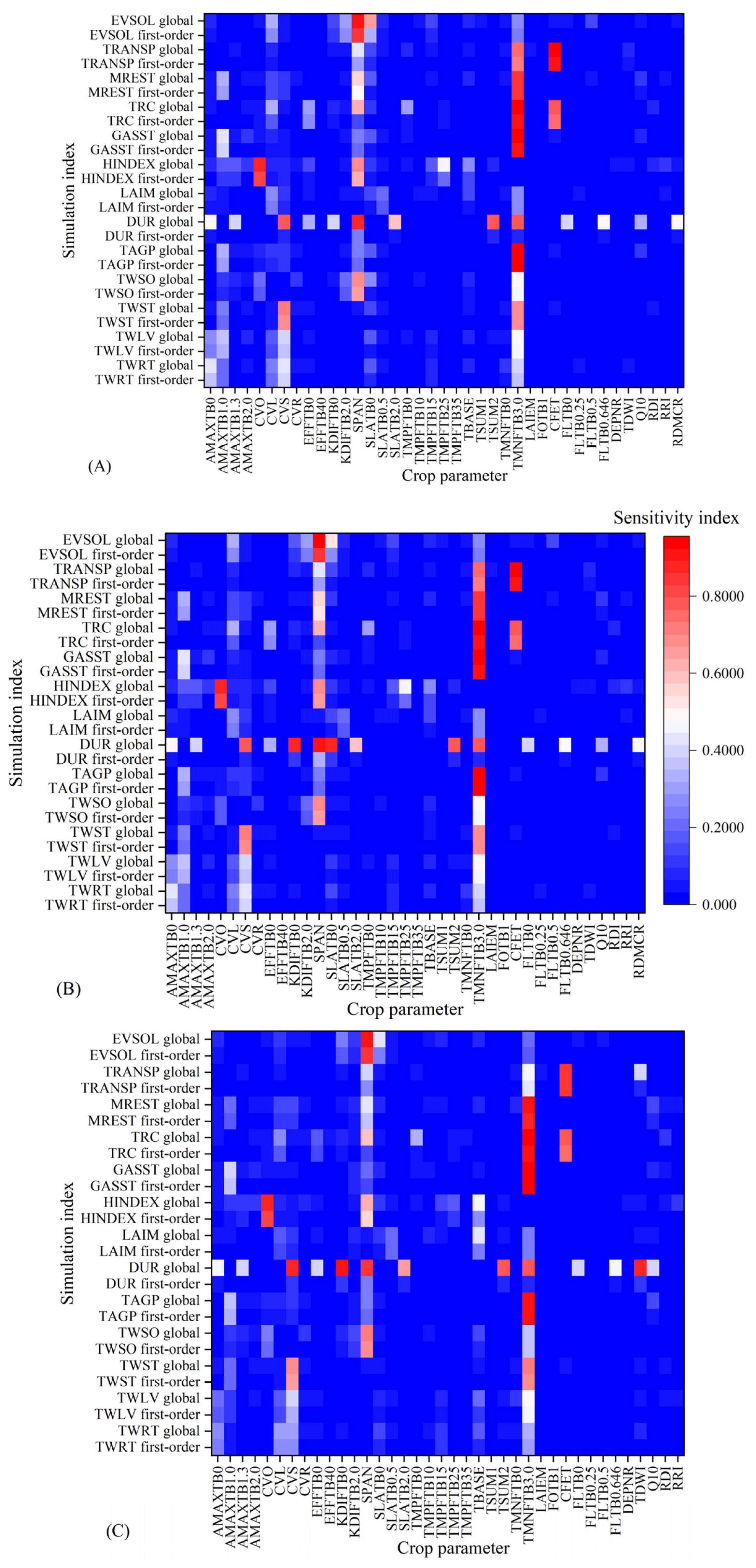
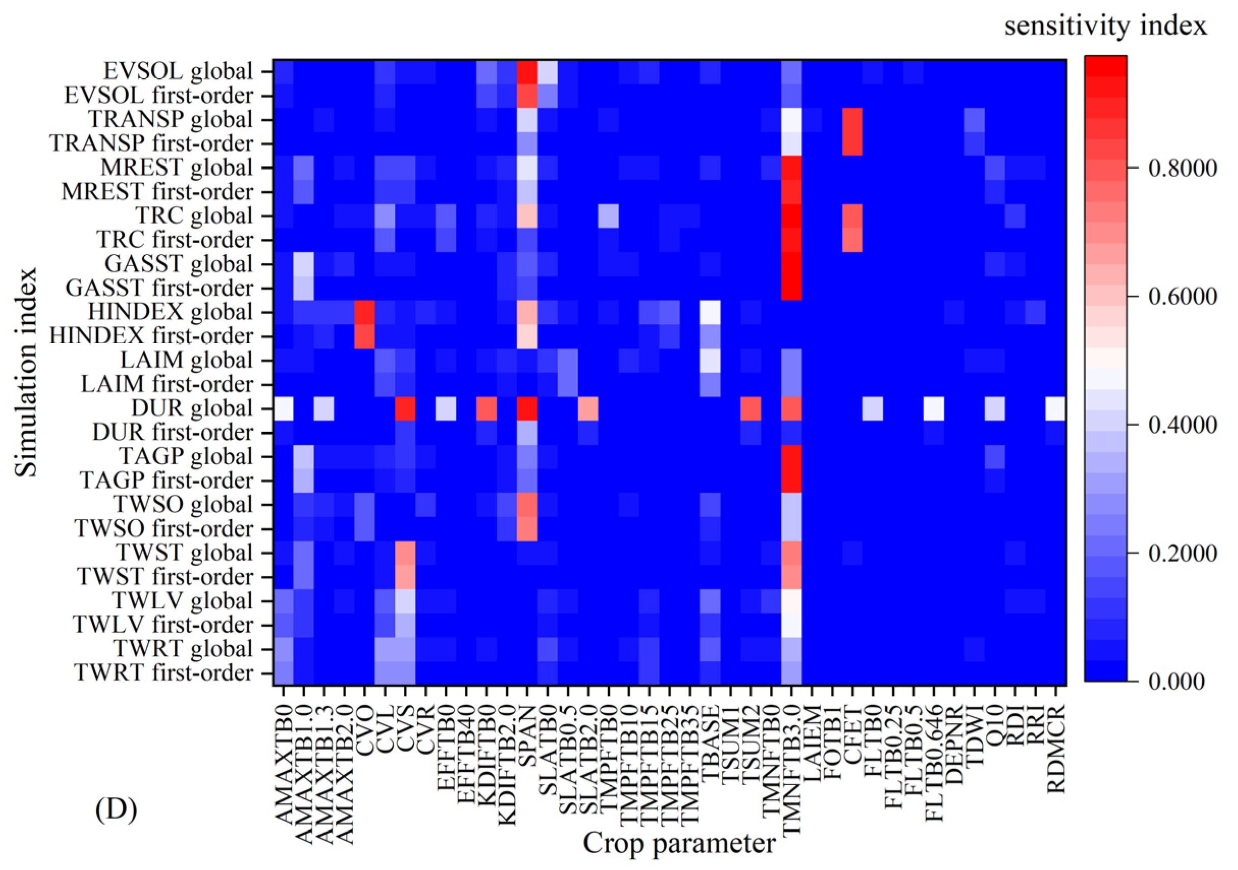
Using randomly generated parameters, the model simulation was conducted under four conditions: 2021 and 2022 potential and water-limited supply scenarios. The Monte Carlo algorithm based on the extended Fourier series sensitivity test method analyzed the 15 simulation indicators and their corresponding 39 crop parameters (Figure 2). The results indicate a consistent trend between first-order sensitivity and global sensitivity. TMNFTB3.0, SPAN, SLATB0, and CFET have higher sensitivity indices for most simulation indices, among which TMNFTB3.0 has higher sensitivity indices for TAGP, GASST, TRC, and MREST. The first-order and global sensitivity indices of SPAN to EVSOL and CFET to TRANSP are both >0.7, indicating that these crop parameters are dominant in the simulation of the corresponding indicators and can explain ≥70% of the variance variation of the results. The study conducted by Xing et al. [47] demonstrated that CEFT exhibited the highest sensitivity among crop parameters in relation to wheat yield, with a global sensitivity index of 0.56, which aligns with the findings of this investigation.

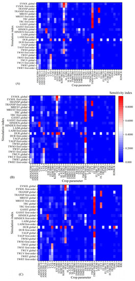
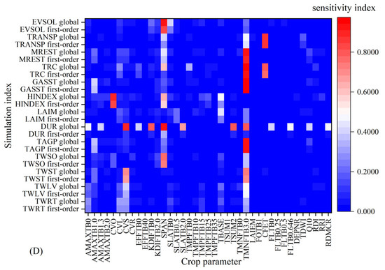
Figure 2. First-order and global sensitivities of crop parameters under the conditions of potential (A), water restriction (B) in 2021, potential (C), and water restriction (D) in 2022.

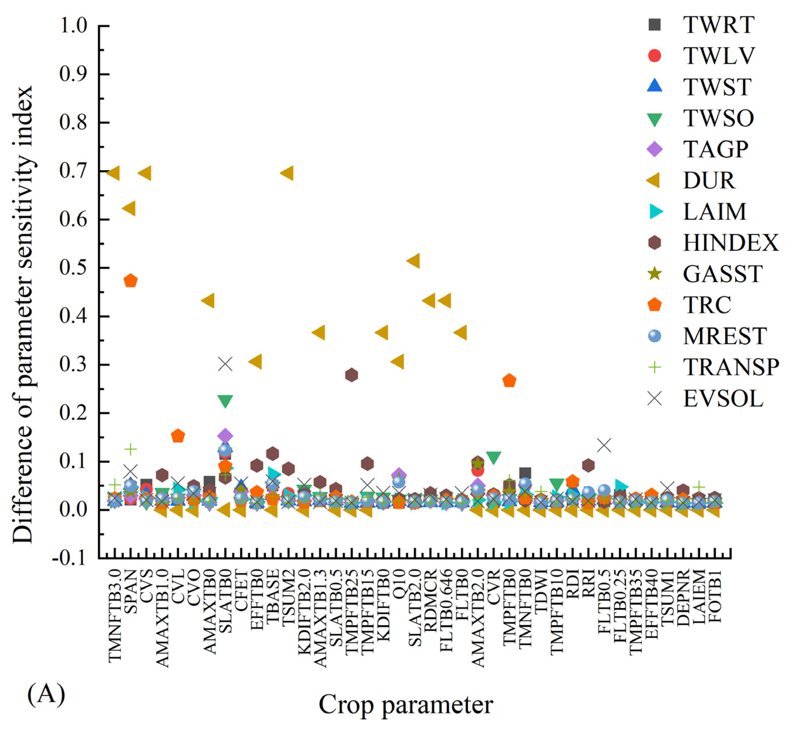
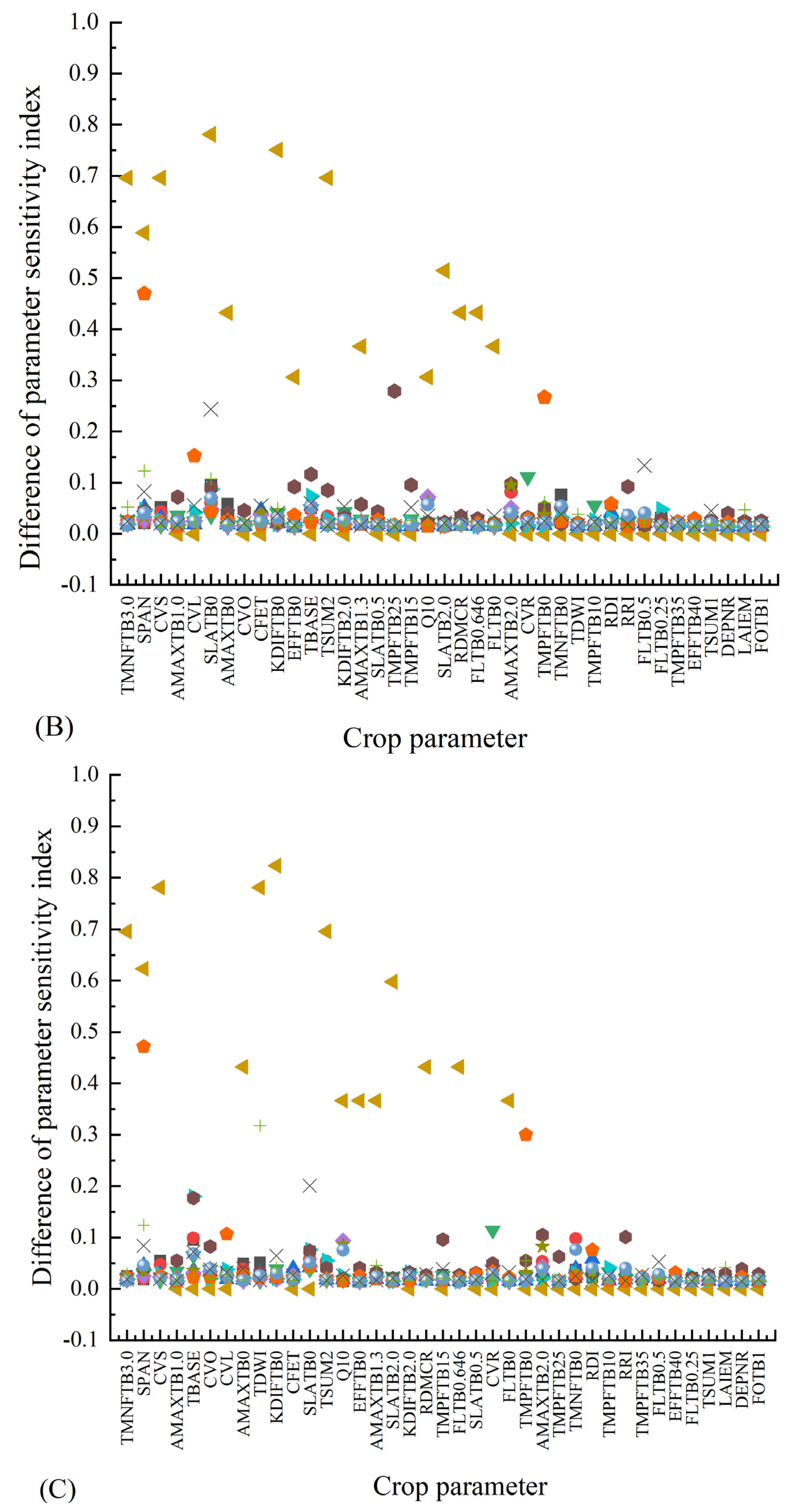
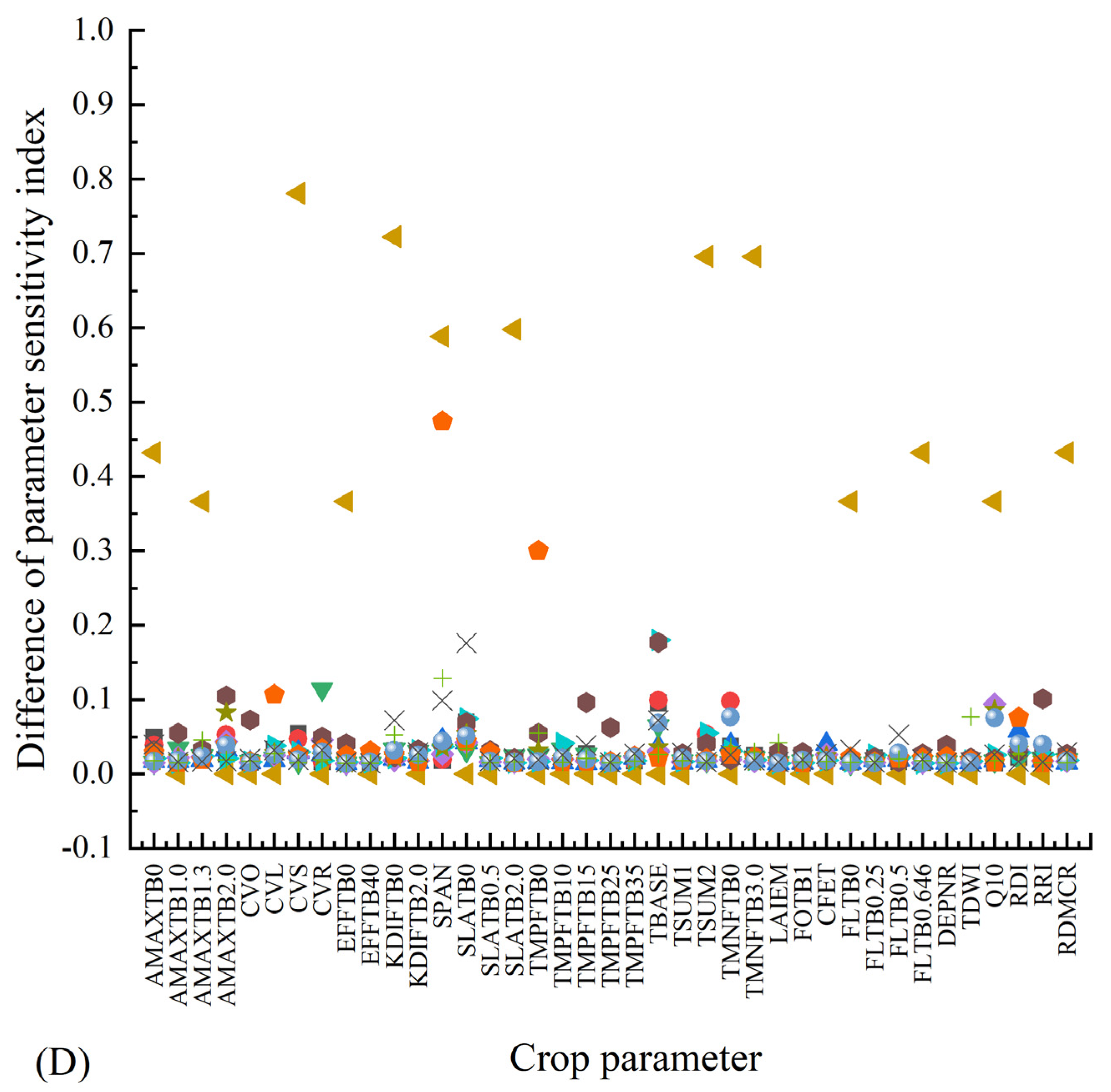
Assuming fixed meteorological, soil and field management conditions, a slight discrepancy exists between first-order sensitivity and global sensitivity of crop parameters for the same model simulation index (Figure 3). The global sensitivity surpasses the first-order sensitivity by a 1–8% margin, except for indicators with negligible disparities in simulation outcomes, such as DUR, where the disparity between first-order and global sensitivity is substantial, exceeding 30%.

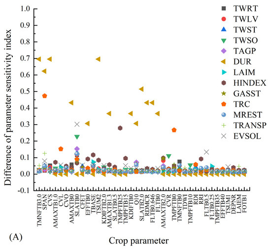
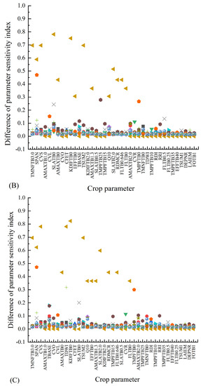
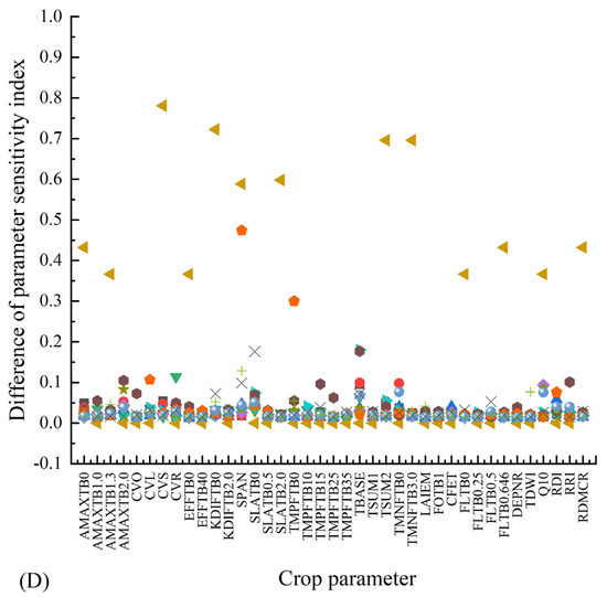
Figure 3. Difference of crop parameter sensitivity under the conditions of potential (A), water restriction (B) in 2021, potential (C) and water restriction (D) in 2022.

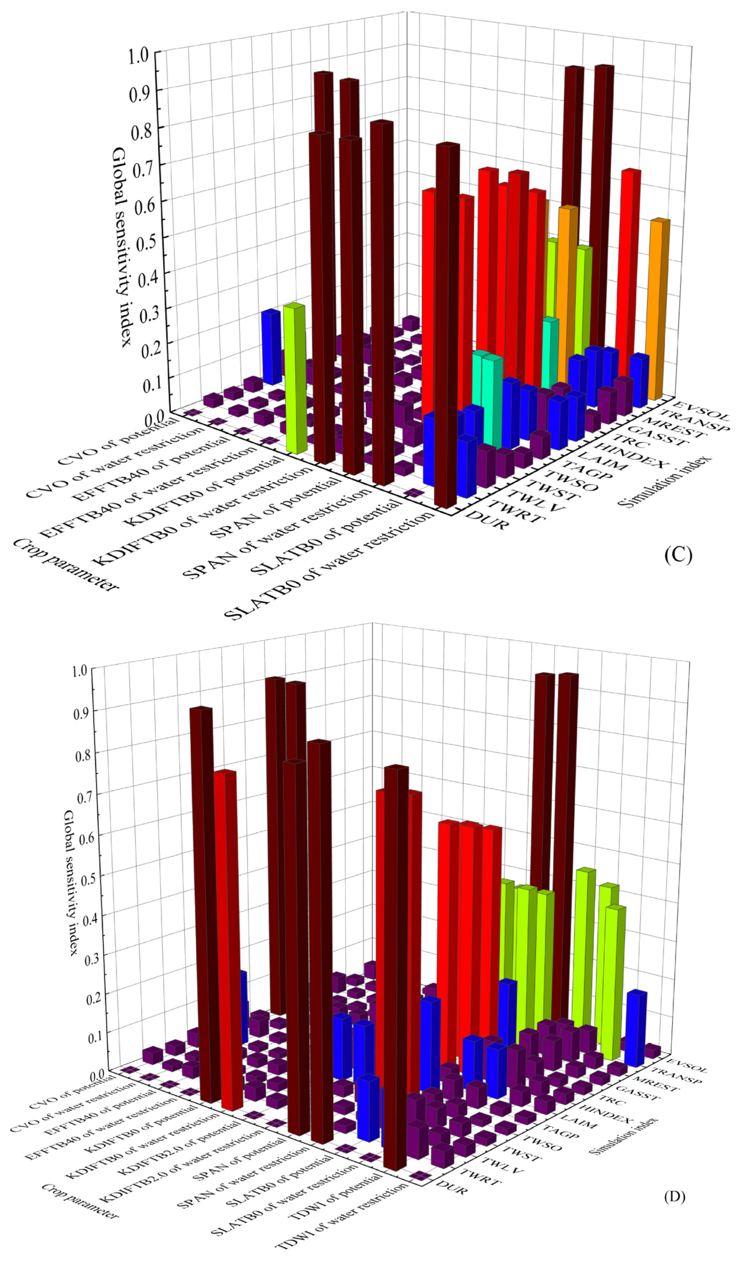
Under identical meteorological conditions, varying water supply has a limited impact on crop parameter sensitivity. In 2021, the changes in water supply only affected the first-order and global sensitivities of five crop parameters: CVO, EFFTB40, KDIFTB0, SPAN, and SLATB0, with those of CVO, EFFTB40, KDIFTB0, KDIFTB2.0, SPAN, SLATB0 and TDWI being impacted by varying water supply conditions in 2022. Among the first-order sensitivities, significant changes are observed for SLATB0 in 2021 and TDW1 in 2022. Notably, KDIFTB0 and SLATB0 exhibited substantial changes in terms of global SA in 2021 (Figure 4).

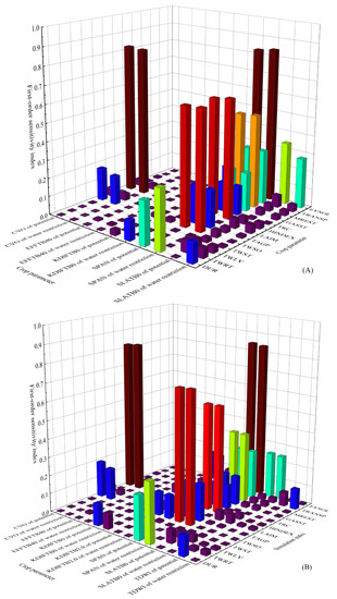
Figure 4. Changes of first-order parameter sensitivity in 2021 (A) and 2022 (B) and changes of global parameter sensitivity in 2021 (C) and 2022 (D).

Under the meteorological conditions of 2021, the sensitivity ranking of wheat yield-related indicators (TWRT, TWLV, TWST, TWSO and TAGP) shows that TMNFTB3.0 > CVS > AMAXTB1.0 > SPAN > AMAXTB0 > CVL exhibited greater sensitivity among crop parameters with slightly varying specific circumstances. SPAN was the most sensitive to TWSO, followed by TMNFTB3.0 and KDIFTB2.0. Furthermore, CVS was the most sensitive to TWRT, followed by AMAXTB0. TMNFTB3.0 was the most sensitive to TAGP, followed by AMAXTB1.0. Changes in the water supply have little effect on the sensitivity ranking of the parameter sensitivity index, with the water limit only affecting the sensitivity ranking of KDIFTB2.0 to TWSO and SLATB0 to TAGP.

Under meteorological conditions of 2022, the ranking of crop parameters with greater sensitivity generally was TMNFTB 3.0 > CVS > SPAN > AMAXTB 1.0 > CVL, similar to 2021. However, there are slight differences in the parameters of crops with greater sensitivity to TWSO. TMNFTB 3.0 > CVO > KDIFTB2.0 > AMAXTB1.0 exhibited a higher global sensitivity to TWST and Q10 to TAGP as compared to first-order sensitivity, while the sensitivity ranking of crop parameters remained unaffected by changes in water supply conditions.

For crop growth-related indices DUR, LAIM, HINDEX, and GASST under the meteorological conditions of 2021, the crop parameters with greater sensitivity are ranked as TMNFTB3.0 > SPAN > CVO > CVS > SLATB0, consistent with the ranking of GASST. Among these parameters, CVL and TMNFTB3.0 have the most significant influence on LAIM, followed by SLATB0.5. CVO is identified as the most influential parameter on HINDEX, followed by SPAN and TMPFTB25. Changes in water supply conditions significantly affect the degree ranking of DUR and the sensitivity index of SLATB0. Under the meteorological circumstances of 2022, TMNFTB3.0 > SPAN > CVO > TBASE > CVS are generally ranked as crop parameters with higher sensitivity, while the rank of HINDEX and GASST exhibited similar parameter sensitivity indices to those observed in 2021. The sensitivity index of crop parameters for LAIM follows the order of TBASE > TMNFTB3.0 > SLATB0.5 > CVL > CVS, with changes in water supply conditions greatly affecting the ranking of parameter degrees for DUR.

In 2021, the evapotranspiration-related indices TRC, MREST, TRANSP, and EVSOL were analyzed under meteorological conditions. The crop parameters with greater sensitivity are ranked as TMNFTB3.0 > SPAN > CFET > SLATB0 > CVL. Specifically, TMNFTB3.0 showed the highest sensitivity to TRC. The second factor is the sensitivity index ranking of various parameters to different environmental stressors. TMNFTB3.0 exhibited the highest sensitivity to MREST, followed by SPAN and AMAXTB1.0. CFET showed the highest sensitivity to TRANSP, followed by TMNFTB3.0 and SPAN. In terms of EVSOL, SPAN had the greatest impact on parameter sensitivity, followed by SLATB0 and CVL. Changes in water supply conditions significantly affected the sensitivity index ranking of SLATB0 but maintained consistent rankings for first-order and global parameters. Under the meteorological conditions of 2022, the sensitivity index ranking slightly differed from that of 2021. Only Q10 and TMPFTB0 displayed a global sensitivity ranking for MREST and TRANSP, respectively, with KDIFTB0 showing a first-order and global sensitivity ranking to EVSOL. Changes in water supply conditions had a negligible effect on the parameter sensitivity index ranking.

In summary, crop parameters with high overall sensitivity often exhibit greater sensitivity towards a single model index, with certain specific parameters possibly displaying higher sensitivity towards particular model indices, thus affecting the parameter sensitivity index ranking. Table A1 lists the detailed rankings. Therefore, when considering model simulation for a specific index, priority should be given to adjusting parameters with the highest sensitivity index ranking.

3.2. SEM of Degree of Contribution of Crop Parameters to Different Simulation Indices

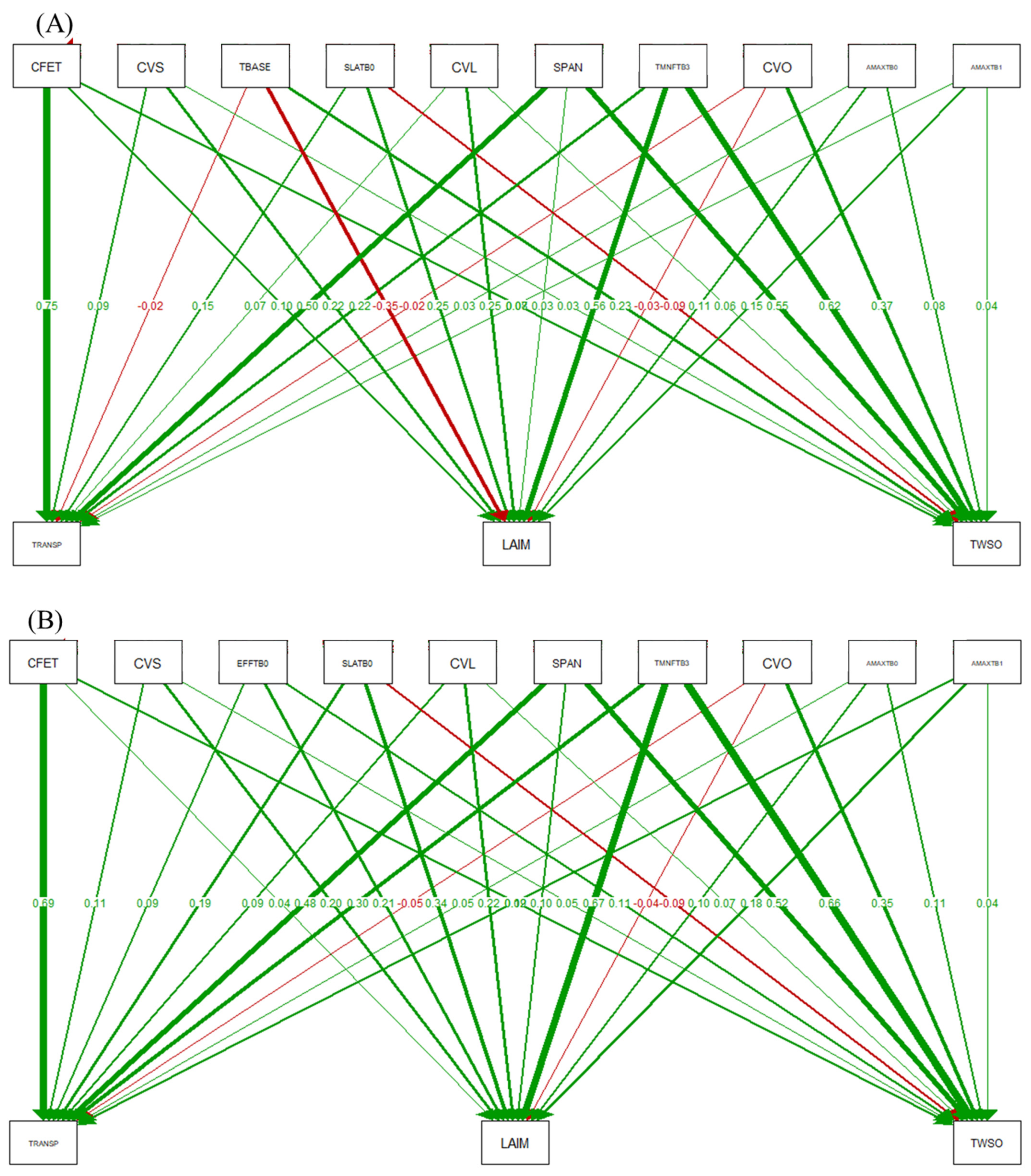
SA conducted a comprehensive selection of 11 representative crop parameters: CEFT, CVS, TBASE, EFFTB0, SLATB0, CVL, SPAN, TMNFTB3.0, CVO, AMAXTB0, and AMAXTB1. TRANSP was chosen as the representative evapotranspiration index, while LAIM and TWSO represented the crop growth index and yield, respectively. These parameters were analyzed using a SEM. The SEM diagram under varying water supply conditions is omitted (Figure 5), as different water supply conditions minimally affect the contribution of crop parameters to simulation indicators, TRANSP, LAIM and TWSO.

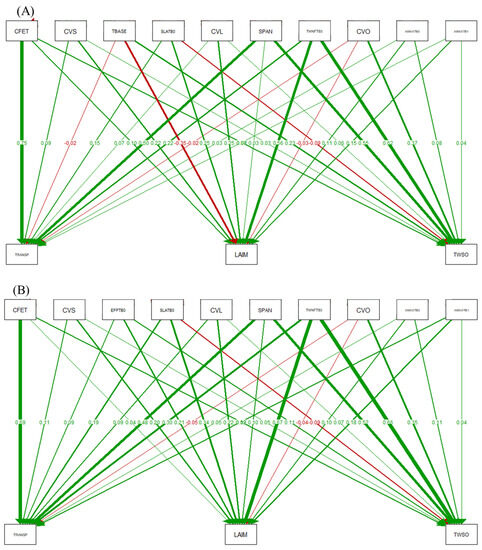
Figure 5. SEM of spring wheat in Yinchuan in 2021 (A) and 2022 (B).

The model demonstrated that CFET had the highest path coefficients of 0.69 and 0.75, followed by SPAN with path coefficients of 0.48 and 0.5, indicating they independently affected the evapotranspiration index TRANSP at rates of 69%, 75%, 48%, and 50%, respectively. Conversely, CVO negatively contributed to TRANSP. Furthermore, TMNFTB3, with path coefficients of 0.67 and 0.56, significantly impacted LAIM and independently accounted for 67% and 56% of the changes in LAIM, respectively. Negative contribution parameters are identified as CVO and TBASE. Regarding the yield index TWSO, TMNFTB3 had the highest impact with path coefficients of 0.66 and 0.62, followed by SPAN with path coefficients of 0.52 and 0.55, independently affecting 66%, 62%, 52%, and 55% of TWSO changes, respectively. However, SLATB0 has a negative contribution. Therefore, these results indicate that diverse meteorological conditions exert varying impacts on the positive and negative degrees of crop parameters’ contributions while negligibly affecting the ranking of parameter contribution degrees.

3.3. Adaptability Verification of the Modified WOFOST Model in the Ningxia Yellow River Irrigation Area

Crop parameters are adjusted based on the growth, development, and yield of spring wheat in Yinchuan in 2021 as a benchmark. Considering actual weather conditions and soil data from other research sites, the simulation results obtained are as follows (Table 3):

Table 3. Parameter values of WOFOST model crops.

Crop Parameter	Value	Crop Parameter	Value	Crop Parameter	Value	Crop Parameter	Value
AMAXTB0	35.2528	CVS	0.724642	KDIFTB2	0.654335	TMPFTB0	0.099835
AMAXTB1	39.0031	CVR	0.667882	SPAN	33.0204	TMPFTB10	0.56683
AMAXTB1.3	38.1757	EFFTB0	0.487338	SLATB0	0.002004	TMPFTB15	0.937174
CVO	0.765686	EFFTB40	0.476887	SLATB0.5	0.001944	TMPFTB25	0.956712
CVL	0.667321	KDIFTB0	0.573685	SLATB2	0.002072	TMPFTB35	0.015039
TBASE	−1.53077	LAIEM	0.129034	FLTB0.5	0.450768	RDI	11.9468
TSUM1	1269.89	FOTB1	0.956577	FLTB0.646	0.296593	RRI	1.29025
TSUM2	1263.68	CFET	0.929755	DEPNR	4.64869	RDMCR	122.543
TMNFTB0	0.078391	FLTB0	0.601276	TDWI	182.62	AMAXTB2	4.84661
TMNFTB3	0.913048	FLTB0.25	0.641849	Q10	1.87027

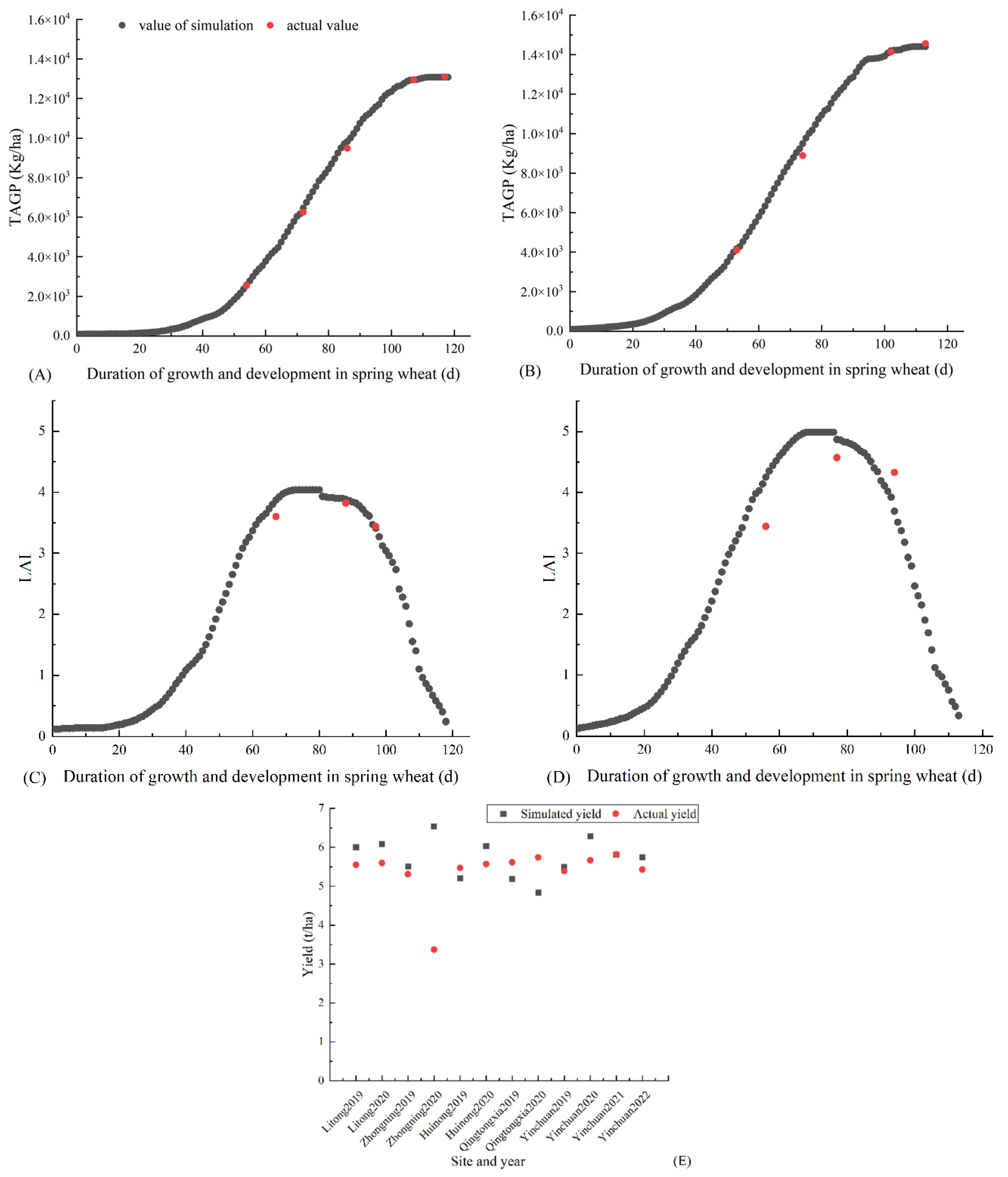
For TAGP simulation using field trials in Yongning County, Yinchuan City, during 2021 and 2022, the model evaluation standards were: $R_{MSE}$ = 0.2516; $M_{BE}$ = 0.1392; $R^2$ = 0.9976. Similarly, for LAI simulation using field trials in Yongning County during 2021 and 2022, the model evaluation standards were: $R_{MSE}$ = 0.4533; $M_{BE}$ = 0.1283; $R^2$ = 0.2877. Finally, Figure 6 shows the simulated outputs for Yinchuan (2019–2022) and Zhongning, Qingtongxia, Litong and Huinong (2019–2020). Thus, the simulation demonstrates that the dry matter accumulation of spring wheat in Yongning County, Yinchuan City (with an error rate below 7%) outperforms the leaf area index (with an error rate below 20%). The rectified model can simulate the Yellow River diversion irrigation region in Ningxia with a <8% deviation.

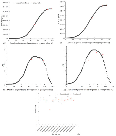
Figure 6. The fitting of TAGP (A), LAI (C), TAGP (B), and LAI (D) in 2021 in Yongning County, Yinchuan City, and the fitting of yield (E) simulation in other regions.

4. Discussion

4.1. Analysis of Crop Parameter Sensitivity and its Response to Different Water Supply Conditions

In this study, EFAST was used to analyze the sensitivity indices of 39 WOFOST crop parameters with respect to 13 model simulation outputs under potential and water-limited conditions. The results indicate that among the yield-related outputs, TMNFTB3.0, CVS, AMAXTB1.0, and SPAN showed the highest sensitivity indices. Furthermore, moisture restriction increases the sensitivity index of AMAXTB0 while decreasing that of SLATB0. Regarding growth-related indices, TMNFTB3.0, SPAN, CVO, TBASE, and SLATB0 exhibit the highest sensitivity index values. Additionally, meteorological conditions in different years significantly impact the sensitivity index. Moisture restriction increases the sensitivity index of SLATB0 and SPAN while decreasing that of CVO.

Regarding evapotranspiration-related indices, TMNFTB3.0, SPAN, CEFT, SLATB0 and CVL exhibited the highest sensitivity levels. However, water restriction reduces the sensitivity index for SLATB0. These findings highlight the crucial role of crop parameters like TMNFTB3.0, SPAN, CVS, and AMAXTB1.0 in spring wheat’s growth and development. Water restriction significantly impacts growth-related indicators, particularly leaf aging, leaf area, and assimilate conversion to storage organs. These findings align with those of a previous report [62]. Leaf senescence, initial specific leaf area, and assimilation rate at 30 °C significantly impact crop yield, growth, and evapotranspiration. The allocation of assimilates to stems, storage organs, and leaves also impacts crop yield, growth, and evapotranspiration. The CO₂ assimilation rate, the low-temperature threshold for leaf aging, and the correction factor for evapotranspiration independently and significantly impact crop yield, growth, and evapotranspiration. This aligns with Xing et al. [47] and underscores the sensitivity and importance of these parameters, as demonstrated previously [62]. Currently, in this study, the parameter CFET, often overlooked in most SA studies, significantly affects crop yield under water-limited conditions. Therefore, accurate verification of this parameter can be highly valuable for simulating crop yield in the Yellow River diversion irrigation area.

Zhang et al. [63] identified TSUM1, FRTB, CVO, CVS, DVSI, SPAN, and SLATB as higher sensitivity parameters in the WOFOST model. The global sensitivity index exceeds 0.5. Similarly, Chen et al. [45] found that TSUM1, SLATB1, SLATB2, SPAN, EFFTB3 and TMPF4 were more sensitive parameters of the WOFOST models. Their global sensitivity indexes were 0.271, 0.237, 0.49, 0.191, 0.126 and 0.149. However, Li et al. [53] reported that SPAN was the most sensitive parameter for dry matter accumulation, differing slightly from the results of this study. This discrepancy might be attributed to crop type and study area variations, as varying crop types could generate different value ranges for different parameters. Xu et al. [64] demonstrated that leaf area index (SLATB), maximum leaf assimilation rate (AMAXTB), and extinction coefficient (KDIFTB2.0) were more sensitive to varying water conditions due to the WOFOST model’s canopy division into distinct leaf layers for calculating each layer’s assimilation rate. Consequently, upper leaves easily achieve their maximum assimilation rates under stronger radiation. Since the light energy utilization efficiency is reduced, particularly in water-scarce conditions where parameter sensitivity changes are more pronounced [65], this aligns with this study’s findings. Furthermore, [45] discovered minimal disparity in the maximum leaf area and above-ground biomass sensitivity to parameters under potential and water-limited cultivation supply conditions. This may be attributed to regional scale, simulated meteorological conditions, and environment or field management measures. This also highlights the significance of conducting SA before model implementation in a specific operational context [66].

4.2. Analysis of Degree of Contribution of SEM to Model Parameters

SA improves the understanding of process variables in a model [66], while SEM visually illustrates the impact of different parameters on various simulation outcomes. The findings indicate that CFET, followed by SPAN and CVO, significantly impacts the evapotranspiration index TRANSP, indicating that higher assimilate conversion to storage organs causes lower evapotranspiration. TMNFTB3, followed by SPAN, has the greatest impact on LAIM and TWSO, highlighting their significant contribution to wheat growth and yields. This finding aligns with the EFAST SA results mentioned above, reinforcing our conclusion. Notably, few studies have reported SEM-based SA of the WOFOST model. However, Wu et al. [67] used SEM analysis to examine the impact of meteorological drought conditions on wheat yield and investigated how climate change and human activities contributed to meteorological droughts and affected the net wheat primary production loss. Temperature, wind, and total solar radiation emerged as primary drivers of agricultural drought due to their high correlation with evapotranspiration. Dewitt et al. [68] utilized SEM to construct an SEM based on yield components and plant growth data. They deciphered the relationship between quantitative trait loci, yield components, and total panicle yield. They also explored how diverse developmental processes that interacted with the environment impacted wheat yield and plant growth. Additionally, Vargas et al. [69] used SEM to analyze the effects of wheat genotypes and climate variables on wheat growth and development. They found that external climate variables were related to the final yield composition, with most process variables like ear number being affected by low temperature and radiation during the early stage of plant development.

4.3. Localization of the WOFOST Model

The localized WOFOST model demonstrated superior reliability in wheat yield prediction compared to its non-localized counterpart, as validated against official statistical wheat yield data. This aligns with previous research findings [70], highlighting the effectiveness of data localization in reducing wheat yield prediction errors. Although the calibration of crop parameters and meteorological conditions improved overall model performance, further enhancements are required for water-related aspects. Notably, simulations of potential crop yield showed a slightly better correlation with recorded yields than those under water-limited conditions [62]. This discrepancy may be attributed to various extreme processes, including the impact of hot and dry winds, waterlogging, pest infestations, diseases, weeds, and field management challenges, which can potentially reduce crop growth and yields.

However, some modeling studies have not fully addressed the impact of extreme weather events on crop production [71]. Extreme events, such as heat waves, cold snaps, droughts, floods, and frosts, directly and indirectly, affect crop systems by altering plant physiology and behavior, growth periods, product quality, and yield [72]. To address this issue, most current crop models require adjustments or updates to formalize the biophysical interactions between crops and their environment, inevitably increasing the number of input factors (variables and parameters) needed for the model to account for this complex interaction. It also involves parameter value distribution intervals, driving variables (climate, soil, and management), and model structure [73]. Therefore, conducting SA is crucial to adapt the model to a specific environment. Moreover, performing SA on the model under various production levels and complex influencing factors can provide deeper insights into the model and enhance its regional applicability.

The development of the WOFOST model is based on the agricultural planting conditions in Europe, so the simulation effect of the adjusted model in other regions is not very ideal, which may be caused by the different meteorological and geographical conditions in the different areas and the different ability of crops to resist cold and drought. Therefore, we suggest that in the actual implementation process, local crops’ yield and planting conditions over the years should be referred to determine and calibrate the model parameters. In addition, sub-models of the impact of pests and weed competition can be considered in the development process of the model.

5. Conclusions

(1)

The first-order and global sensitivity trends of spring wheat parameters in the WOFOST model showed consistent results. TMNFTB3.0, SPAN, SLATB0, and CFET exhibited higher sensitivity for most simulation indices. The impact of different water supply conditions on crop parameter sensitivity in the WOFOST model was limited under identical meteorological conditions. SA of crop parameters in the WOFOST model revealed that TMNFTB3.0, SPAN, CVS, AMAXTB1.0 and other crop parameters significantly affect the growth and development of spring wheat. Furthermore, water restriction severely impacted the growth-related indices, particularly leaf senescence, leaf area, and the assimilate allocation to storage organs.

(2)

The SEM identified CFET is the crop parameter with the highest contribution to the evapotranspiration index TRANSP, while TMNFTB3 have the highest impact on LAIM. TMNFTB3 is the most influential crop parameter for the yield index TWSO.

(3)

The TAGP simulation results from field trials conducted in Yongning County, Yinchuan City, during 2021 and 2022 met the model evaluation standards as evident from $R_{MSE}$ = 0.2516; $M_{BE}$ = 0.1392; $R^2$ = 0.9976. For LAI results from the same field trials, the model evaluation standards were: $R_{MSE}$ = 0.4533; $M_{BE}$ = 0.1283; $R^2$ = 0.2877. Therefore, the corrected model demonstrates improved simulation accuracy for the Ningxia Yellow River diversion irrigation area, with errors <8%.

References

- Zhao, J.; Pu, F.; Li, Y.; Xu, J.; Li, N.; Zhang, Y.; Guo, J.; Pan, Z. Assessing the combined effects of climatic factors on spring wheat phenophase and grain yield in inner mongolia, China. PLoS ONE 2017, 12, e185690. [Google Scholar] [CrossRef]
- Osborne, T.M.; Lawrence, D.M.; Challinor, A.J.; Slingo, J.M.; Wheeler, T.R. Development and assessment of a coupled crop–climate model. Glob. Chang. Biol. 2007, 13, 169–183. [Google Scholar] [CrossRef]
- Bowerman, A.F.; Newberry, M.; Dielen, A.; Whan, A.; Larroque, O.; Pritchard, J.; Gubler, F.; Howitt, C.A.; Pogson, B.J.; Morell, M.K.; et al. Suppression of glucan, water dikinase in the endosperm alters wheat grain properties, germination and coleoptile growth. Plant Biotechnol. J. 2016, 14, 398–408. [Google Scholar] [CrossRef] [PubMed]
- Zhai, Z.; Martínez, J.F.; Beltran, V.; Martínez, N.L. Decision support systems for agriculture 4.0: Survey and challenges. Comput. Electron. Agric. 2020, 170, 105256. [Google Scholar] [CrossRef]
- Gaydon, D.S.; Balwinder-Singh Wang, E.; Poulton, P.L.; Ahmad, B.; Ahmed, F.; Akhter, S.; Ali, I.; Amarasingha, R.; Chaki, A.K.; Chen, C.; et al. Evaluation of the apsim model in cropping systems of Asia. Field Crops Res. 2017, 204, 52–75. [Google Scholar] [CrossRef]
- Ceglar, A.; van der Wijngaart, R.; de Wit, A.; Lecerf, R.; Boogaard, H.; Seguini, L.; van den Berg, M.; Toreti, A.; Zampieri, M.; Fumagalli, D.; et al. Improving wofost model to simulate winter wheat phenology in europe: Evaluation and effects on yield. Agric. Syst. 2019, 168, 168–180. [Google Scholar] [CrossRef]
- Leghari, S.J.; Hu, K.; Liang, H.; Wei, Y. Modeling water and nitrogen balance of different cropping systems in the north China plain. Agronomy 2019, 9, 696. [Google Scholar] [CrossRef]
- Shahhosseini, M.; Hu, G.; Huber, I.; Archontoulis, S.V. Coupling machine learning and crop modeling improves crop yield prediction in the us corn belt. Sci. Rep. 2021, 11, 1606. [Google Scholar] [CrossRef]
- Zhang, Y.; Li, S.; Wu, M.; Yang, D.; Wang, C. Study on the response of different soybean varieties to water management in northwest China based on a model approach. Atmosphere 2021, 12, 824. [Google Scholar] [CrossRef]
- Bregaglio, S.; Donatelli, M.; Confalonieri, R.; Acutis, M.; Orlandini, S. Multi metric evaluation of leaf wetness models for large-area application of plant disease models. Agric. For. Meteorol. 2011, 151, 1163–1172. [Google Scholar] [CrossRef]
- Heng, L.K.; Hsiao, T.; Evett, S.; Howell, T.; Steduto, P. Validating the fao aquacrop model for irrigated and water deficient field maize. Agron. J. 2009, 101, 488–498. [Google Scholar] [CrossRef]
- Liang, H.; Hu, K.; Batchelor, W.D.; Qin, W.; Li, B. Developing a water and nitrogen management model for greenhouse vegetable production in China: Sensitivity analysis and evaluation. Ecol. Model. 2018, 367, 24–33. [Google Scholar] [CrossRef]
- Makler-Pick, V.; Gal, G.; Gorfine, M.; Hipsey, M.R.; Carmel, Y. Sensitivity analysis for complex ecological models—A new approach. Environ. Model. Softw. 2011, 26, 124–134. [Google Scholar] [CrossRef]
- Stella, T.; Frasso, N.; Negrini, G.; Bregaglio, S.; Cappelli, G.; Acutis, M.; Confalonieri, R. Model simplification and development via reuse, sensitivity analysis and composition: A case study in crop modelling. Environ. Model. Softw. 2014, 59, 44–58. [Google Scholar] [CrossRef]
- Tan, J.; Cui, Y.; Luo, Y. Global sensitivity analysis of outputs over rice-growth process in Oryza model. Environ. Model. Softw. 2016, 83, 36–46. [Google Scholar] [CrossRef]
- Corbeels, M.; Chirat, G.; Messad, S.; Thierfelder, C. Performance and sensitivity of the dssat crop growth model in simulating maize yield under conservation agriculture. Eur. J. Agron. 2016, 76, 41–53. [Google Scholar] [CrossRef]
- Tao, S.; Shen, S.; Li, Y.; Wang, Q.; Gao, P.; Mugume, I. Projected crop production under regional climate change using scenario data and modeling: Sensitivity to chosen sowing date and cultivar. Sustainability 2016, 8, 214. [Google Scholar] [CrossRef]
- Ojeda, J.J.; Volenec, J.J.; Brouder, S.M.; Caviglia, O.P.; Agnusdei, M.G. Evaluation of agricultural production systems simulator as yield predictor of Panicum virgatum and Miscanthus x giganteus in several us environments. Glob. Chang. Biol. Bioenergy 2017, 9, 796–816. [Google Scholar] [CrossRef]
- Borgonovo, E.; Plischke, E. Sensitivity analysis: A review of recent advances. Eur. J. Oper. Res. 2016, 248, 869–887. [Google Scholar] [CrossRef]
- Wallach, D.; Thorburn, P.J. Estimating uncertainty in crop model predictions: Current situation and future prospects. Eur. J. Agron. 2017, 88, A1–A7. [Google Scholar] [CrossRef]
- Varella, H.; Guérif, M.; Buis, S. Global sensitivity analysis measures the quality of parameter estimation: The case of soil parameters and a crop model. Environ. Model. Softw. 2010, 25, 310–319. [Google Scholar] [CrossRef]
- Abbate, P.E.; Dardanelli, J.L.; Cantarero, M.G.; Maturano, M.; Melchiori, R.J.M.; Suero, E.E. Climatic and water availability effects on water-use efficiency in wheat. Crop Sci. 2004, 44, 474–483. [Google Scholar] [CrossRef]
- Song, M.D.; Feng, H.; Li, Z.P.; Gao, J.E. Sensitivity analysis of ceres-wheat model based on morris and efast. Chin. J. Agric. Mach. 2014, 45, 124–131. [Google Scholar]
- Xiao, Y.; Zhao, W.; Zhou, D.; Gong, H. Sensitivity analysis of vegetation reflectance to biochemical and biophysical variables at leaf, canopy, and regional scales. IEEE Trans. Geosci. Remote Sens. 2014, 52, 4014–4024. [Google Scholar] [CrossRef]
- Sobol, I.M. Global sensitivity indices for nonlinear mathematical models and their Monte Carlo estimates. Math. Comput. Simul. 2001, 55, 271–280. [Google Scholar] [CrossRef]
- Cui, J.T.; Shao, G.C.; Lin, J.; Ding, M.M. Global sensitivity analysis of parameters of cropgro-tomato model based on efast. J. Agric. Mach. 2020, 51, 237–244. [Google Scholar]
- Wu, J.; Yu, F.S.; Chen, Z.X.; Chen, J. Global sensitivity analysis of winter wheat growth simulation parameters based on epic model. Chin. J. Agric. Eng. 2009, 25, 136–142. [Google Scholar]
- Wang, J.; Li, X.; Lu, L.; Fang, F. Parameter sensitivity analysis of crop growth models based on the extended Fourier amplitude sensitivity test method. Environ. Model. Softw. 2013, 48, 171–182. [Google Scholar] [CrossRef]
- Confalonieri, R. Monte Carlo based sensitivity analysis of two crop simulators and considerations on model balance. Eur. J. Agron. 2010, 33, 89–93. [Google Scholar] [CrossRef]
- Dejonge, K.C.; Ascough, J.C.; Ahmadi, M.; Andales, A.A.; Arabi, M. Global sensitivity and uncertainty analysis of a dynamic agroecosystem model under different irrigation treatments. Ecol. Model. 2012, 231, 113–125. [Google Scholar] [CrossRef]
- Lei, G.; Zeng, W.; Jiang, Y.; Ao, C.; Wu, J.; Huang, J. Sensitivity analysis of the swap (soil-water-atmosphere-plant) model under different nitrogen applications and root distributions in saline soils. Pedosphere 2021, 31, 807–821. [Google Scholar] [CrossRef]
- Vanuytrecht, E.; Raes, D.; Steduto, P.; Hsiao, T.C.; Fereres, E.; Heng, L.K.; Garcia Vila, M.; Mejias Moreno, P. Aquacrop: Fao’s crop water productivity and yield response model. Environ. Model. Softw. 2014, 62, 351–360. [Google Scholar] [CrossRef]
- Brun, R.; Reichert, P.; Kuensch, H.R. Practical identifiability analysis of large environmental simulation models. Water Resour. Res. 2001, 37, 1015–1030. [Google Scholar] [CrossRef]
- Confalonieri, R.; Bellocchi, G.; Tarantola, S.; Acutis, M.; Donatelli, M.; Genovese, G. Sensitivity analysis of the rice model warm in europe: Exploring the effects of different locations, climates and methods of analysis on model sensitivity to crop parameters. Environ. Model. Softw. 2010, 25, 479–488. [Google Scholar] [CrossRef]
- Pastres, R.; Ciavatta, S. A comparison between the uncertainties in model parameters and in forcing functions: Its application to a 3D water-quality model. Environ. Model. Softw. 2005, 20, 981–989. [Google Scholar] [CrossRef]
- Wu, D.R.; Ouyang, Z.; Zhao, X.M.; Yu, Q.; Luo, Y. Applicability of crop growth model Wofost in North China Plain. Chin. J. Plant Ecol. 2003, 27, 594–602. [Google Scholar]
- Xie, W.X.; Wang, G.H.; Zhang, Q.C. Development and application of Wofost model. Chin. J. Soil Sci. 2006, 1, 154–158. [Google Scholar]
- Zhu, J.H.; Dai, P.; Zhu, K.Q.; Chen, Y.; Fan, Y.C.; Li, J.; Feng, D.L.; Qu, H.Q. Research progress of Wofost model. J. Anhui Agric. Sci. 2016, 44, 194–196. [Google Scholar]
- Wang, W.-B.; Wang, J.-M.; Fan, Y.-Y.; Chen, J.; Miles, D.; Jin, H.-J.; He, H.-L. Evaluation of simulation performance of soil water characteristic curve model. J. Glaciol. Geocryol. 2019, 41, 1448–1455. [Google Scholar]
- Schaap, M.G.; Leij, F.J.; van Genuchten, M.T. Rosetta: A computer program for estimating soil hydraulic parameters with hierarchical pedotransfer functions. J. Hydrol. 2001, 251, 163–176. [Google Scholar] [CrossRef]
- Wang, L.; Weng, X.; Yao, Z.; Zhang, R.; Li, W.; Li, Y. Segmental modification of the mualem model by remolded loess. Math. Probl. Eng. 2017, 2017, 2768952. [Google Scholar] [CrossRef]
- Esfandiari, A. An innovative sensitivity-based method for structural model updating using incomplete modal data. Struct. Control Health Monit. 2017, 24, e1905. [Google Scholar] [CrossRef]
- Amini, A.; Alimohammadlou, M. Toward equation structural modeling: An integration of interpretive structural modeling and structural equation modeling. J. Manag. Anal. 2021, 8, 693–714. [Google Scholar] [CrossRef]
- Grace, J.B.; Anderson, T.M.; Olff, H.; Scheiner, S.M. On the specification of structural equation models for ecological systems. Ecol. Monogr. 2010, 80, 67–87. [Google Scholar] [CrossRef]
- Chen, Y.L.; Gu, X.H.; Gong, A.D. Parameter sensitivity analysis of Wofost crop model based on efast method. J. Henan Polytech. Univ. 2018, 37, 72–78. [Google Scholar]
- He, L.; Hou, Y.Y.; Zhao, G.; Wu, D.R.; Yu, Q. Parameter optimization of Wofost crop model based on global sensitivity analysis and Bayesian method. Chin. J. Agric. Eng. 2016, 32, 169–179. [Google Scholar]
- Xing, A.; Zhuo, Z.Q.; Zhao, Y.Z.; Li, Y.; Huang, Y.F. Parameter sensitivity analysis of Wofost model at different production levels based on efast. Chin. J. Agric. Mach. 2020, 51, 161–171. [Google Scholar]
- Saltelli, A.; Tarantola, S.; Chan, K.P.S. A quantitative model-independent method for global sensitivity analysis of model output. Technometrics 1999, 41, 39. [Google Scholar] [CrossRef]
- Scollo, S.; Tarantola, S.; Bonadonna, C.; Coltelli, M.; Saltelli, A. Sensitivity analysis and uncertainty estimation for tephra dispersal models. J. Geophys. Res. 2008, 113, 4864. [Google Scholar] [CrossRef]
- Chan, I.S.; Goldstein, A.A.; Bassingthwaighte, J.B. Sensop: A derivative-free solver for nonlinear least squares with sensitivity scaling. Ann. Biomed. Eng. 1993, 21, 621–631. [Google Scholar] [CrossRef]
- Xing, H.; Xu, X.; Li, Z.; Chen, Y.; Feng, H.; Yang, G.; Chen, Z. Global sensitivity analysis of the aquacrop model for winter wheat under different water treatments based on the extended Fourier amplitude sensitivity test. J. Integr. Agric. 2017, 16, 2444–2458. [Google Scholar] [CrossRef]
- Dimov, I.; Georgieva, R.; Ostromsky, T. Monte Carlo sensitivity analysis of an Eulerian large-scale air pollution model. Reliab. Eng. Syst. Saf. 2012, 107, 23–28. [Google Scholar] [CrossRef]
- Li, Z.; Jin, X.; Liu, H.; Xu, X.; Wang, J. Global sensitivity analysis of wheat grain yield and quality and the related process variables from the dssat-ceres model based on the extended Fourier amplitude sensitivity test method. J. Integr. Agric. 2019, 18, 1547–1561. [Google Scholar] [CrossRef]
- Vazquez-Cruz, M.A.; Guzman-Cruz, R.; Lopez-Cruz, I.L.; Cornejo-Perez, O.; Torres-Pacheco, I.; Guevara-Gonzalez, R.G. Global sensitivity analysis by means of efast and sobol’ methods and calibration of reduced state-variable tomgro model using genetic algorithms. Comput. Electron. Agric. 2014, 100, 1–12. [Google Scholar] [CrossRef]
- Zhang, J.L.; Li, Y.P.; Zeng, X.T.; You, L.; Liu, J. Sensitivity analysis of hydrological process parameters in cold and arid regions based on efast method. S. N. Water Divers. Water Technol. 2017, 15, 43–48. [Google Scholar]
- Gao, J.; Zhou, B.P.; Wang, Y.; Wang, J.; Yu, H. Sensitivity analysis and applicability evaluation of efast based dssat model for cotton parameters in southern Xinjiang. Jiangsu Agric. Sci. 2022, 50, 185–191. [Google Scholar]
- Wang, J.D.; Guo, W.D.; Li, H.Q. Application of extended Fourier amplitude sensitivity test (efast) method in land surface parameter sensitivity analysis. Acta Phys. Sin. 2013, 62, 050202. [Google Scholar] [CrossRef]
- Wang, Z.M.; Zhang, B.; Song, K.S.; Duan, H.T. Calibration and validation of Cropsyst crop model in typical black soil area of Songnen Plain. J. Agric. Eng. 2005, 21, 47–50. [Google Scholar]
- Lv, L.; Liang, S.; Zhang, J.; Yao, Y.; Dong, Z.; Zhang, L.; Jia, X.-L. Response of yield and light use of different wheat varieties to accumulated temperature before winter. J. Wheat Crops 2017, 37, 1047–1055. [Google Scholar]
- Jin, H.; Li, A.; Wang, J.; Bo, Y. Improvement of spatially and temporally continuous crop leaf area index by integration of ceres-maize model and modis data. Eur. J. Agron. 2016, 78, 1–12. [Google Scholar] [CrossRef]
- Cheng, Z.; Meng, J.; Wang, Y. Improving spring maize yield estimation at field scale by assimilating time-series hj-1 ccd data into the wofost model using a new method with fast algorithms. Remote Sens. 2016, 8, 303. [Google Scholar] [CrossRef]
- Gilardelli, C.; Confalonieri, R.; Cappelli, G.A.; Bellocchi, G. Sensitivity of wofost-based modelling solutions to crop parameters under climate change. Ecol. Model. 2018, 368, 1–14. [Google Scholar] [CrossRef]
- Zhang, N.; Zhang, Q.G.; Yu, H.J.; Cheng, M.D.; Dong, S.J. Parametric sensitivity analysis of crop growth simulation models. J. Zhejiang Univ. (Agric. Life Sci.) 2018, 44, 107–115. [Google Scholar]
- Xu, X.; Shen, S.; Xiong, S.; Ma, X.; Fan, Z.; Han, H. Water stress is a key factor influencing the parameter sensitivity of the wofost model in different agro-meteorological conditions. Int. J. Plant Prod. 2021, 15, 231–242. [Google Scholar] [CrossRef]
- Bassu, S.; Brisson, N.; Durand, J.; Boote, K.; Lizaso, J.; Jones, J.W.; Rosenzweig, C.; Ruane, A.C.; Adam, M.; Baron, C.; et al. How do various maize crop models vary in their responses to climate change factors? Glob. Chang. Biol. 2014, 20, 2301–2320. [Google Scholar] [CrossRef]
- Constantin, J.; Raynal, H.; Casellas, E.; Hoffmann, H.; Bindi, M.; Doro, L.; Eckersten, H.; Gaiser, T.; Grosz, B.; Haas, E.; et al. Management and spatial resolution effects on yield and water balance at regional scale in crop models. Agric. For. Meteorol. 2019, 275, 184–195. [Google Scholar] [CrossRef]
- Wu, J.; Gu, Y.; Sun, K.; Wang, N.; Shen, H.; Wang, Y.; Ma, X. Correlation of climate change and human activities with agricultural drought and its impact on the net primary production of winter wheat. J. Hydrol. 2023, 620, 129504. [Google Scholar] [CrossRef]
- Dewitt, N.; Guedira, M.; Murphy, J.P.; Marshall, D.; Mergoum, M.; Maltecca, C.; Brown-Guedira, G. A network modeling approach provides insights into the environment-specific yield architecture of wheat. Genetics 2022, 221, iyac076. [Google Scholar] [CrossRef]
- Vargas, M.; Crossa, J.; Reynolds, M.P.; Dhungana, P.; Eskridge, K.M. Paper presented at international workshop on increasing wheat yield potential, Cimmyt, Obregon, Mexico, 20–24 March 2006 structural equation modelling for studying genotype × environment interactions of physiological traits affecting yield in wheat. J. Agric. Sci. 2007, 145, 151. [Google Scholar] [CrossRef]
- Mishra, V.; Cruise, J.F.; Mecikalski, J.R. Assimilation of coupled microwave/thermal infrared soil moisture profiles into a crop model for robust maize yield estimates over southeast united states. Eur. J. Agron. 2021, 123, 126208. [Google Scholar] [CrossRef]
- Zinyengere, N.; Crespo, O.; Hachigonta, S.; Tadross, M. Local impacts of climate change and agronomic practices on dry land crops in southern africa. Agric. Ecosyst. Environ. 2014, 197, 1–10. [Google Scholar] [CrossRef]
- Horton, R.M.; Mankin, J.S.; Lesk, C.; Coffel, E.; Raymond, C. A review of recent advances in research on extreme heat events. Curr. Clim. Chang. Rep. 2016, 2, 242–259. [Google Scholar] [CrossRef]
- Gabrielle, B.; Laville, P.; Duval, O.; Nicoullaud, B.; Germon, J.C.; Hénault, C. Process-based modeling of nitrous oxide emissions from wheat-cropped soils at the subregional scale. Glob. Biogeochem. Cycles 2006, 20. [Google Scholar] [CrossRef]
Disclaimer/Publisher’s Note: The statements, opinions and data contained in all publications are solely those of the individual author(s) and contributor(s) and not of MDPI and/or the editor(s). MDPI and/or the editor(s) disclaim responsibility for any injury to people or property resulting from any ideas, methods, instructions or products referred to in the content. |
© 2023 by the authors. Licensee MDPI, Basel, Switzerland. This article is an open access article distributed under the terms and conditions of the Creative Commons Attribution (CC BY) license (https://creativecommons.org/licenses/by/4.0/).