An Efficient and Automated Image Preprocessing Using Semantic Segmentation for Improving the 3D Reconstruction of Soybean Plants at the Vegetative Stage

Abstract

The investigation of plant phenotypes through 3D modeling has emerged as a significant field in the study of automated plant phenotype acquisition. In 3D model construction, conventional image preprocessing methods exhibit low efficiency and inherent inefficiencies, which increases the difficulty of model construction. In order to ensure the accuracy of the 3D model, while reducing the difficulty of image preprocessing and improving the speed of 3D reconstruction, deep learning semantic segmentation technology was used in the present study to preprocess original images of soybean plants. Additionally, control experiments involving soybean plants of different varieties and different growth periods were conducted. Models based on manual image preprocessing and models based on image segmentation were established. Point cloud matching, distance calculation and model matching degree calculation were carried out. In this study, the DeepLabv3+, Unet, PSPnet and HRnet networks were used to conduct semantic segmentation of the original images of soybean plants in the vegetative stage (V), and Unet network exhibited the optimal test effect. The values of mIoU, mPA, mPrecision and mRecall reached 0.9919, 0.9953, 0.9965 and 0.9953. At the same time, by comparing the distance results and matching accuracy results between the models and the reference models, a conclusion could be drawn that semantic segmentation can effectively improve the challenges of image preprocessing and long reconstruction time, greatly improve the robustness of noise input and ensure the accuracy of the model. Semantic segmentation plays a crucial role as a fundamental component in enabling efficient and automated image preprocessing for 3D reconstruction of soybean plants during the vegetative stage. In the future, semantic segmentation will provide a solution for the pre-processing of 3D reconstruction for other crops.

1. Introduction

Soybean, being one of the primary global economic crops, represents a vital aspect of meeting the growing demand from the population. As such, plant scientists and breeders face a considerable challenge in improving the productivity and yield of soybean crops to address these escalating demands [1]. The phenotypic information of soybeans is closely related to factors such as yield and quality. Three-dimensional reconstruction technology is a trending research topic in the field of computer vision, allowing for the realistic representation of 3D objects from the real world in a digital form. As a vital tool for quantitative analysis of crop phenotypes, 3D reconstruction is of considerable significance in exploring crop phenotypic characteristics and plant breeding. The combination of information technology and virtual reality technology in agriculture provides an important means for acquiring virtual plants.

At present, methods for obtaining virtual plants through 3D reconstruction generally include:

• Rule-based methods. For instance, Favre et al. [2] developed the L-studio-based simulator, which was used by Kaya Turgut et al. [3] to generate synthetic rose tree models. Despite the method being less affected by environmental factors and having lower reconstruction costs, it has problems such as large errors and low reconstruction accuracy.
• Image-based methods. Zhu et al. [4] established a soybean digital image acquisition platform by employing a multiple-view stereo (MVS) vision system with digital cameras positioned at varying angles. Such an approach effectively addressed the issue of mutual occlusion among soybean leaves, resulting in the acquisition of a sequence of morphological images of the target plant for subsequent 3D reconstruction of soybean plants. Jorge Martinez-Guanter et al. [5] used the Sfm method for model reconstruction. A set of images covering each crop plant was used and the dataset was composed of approximately 30 to 40 images per sample for full coverage of each plant based on its size, thereby guaranteeing a proper reconstruction. Based on MVS technology, Sun et al. [6] reconstructed 3D models of soybean plants and created 102 original models.
• Instrument-based methods. Due to the rapid advancements and widespread adoption of 3D laser scanning technology, researchers and practitioners have begun utilizing scanning techniques to reconstruct accurate crop models. To illustrate, Boxiang Xiao et al. [7] used a 3D digitizer to obtain spatial structure and distribution data of wheat canopy. After data processing, a 3D model of the plant organs was built, including stems and leaves, based on surface modeling algorithms. Laser scanning has emerged as a novel technology and tool for the next generation of plant phenotyping applications [8]. Jingwen Wu et al. [9] successfully generated a 3D point cloud representation of a plant by utilizing a multi-view image sequence as the basis. An optimized iterative closest point registration method was used to calibrate the point cloud data obtained from laser scanning, thereby improving the plant’s detailed features and establishing a 3D model. Instrument-based 3D reconstruction methods can directly capture point cloud data of ground crops at a faster speed [10]. However, such methods also have some challenges such as large cloud data volume, long processing time, high equipment costs and difficulty in point cloud denoising. In consideration of the accuracy, speed and cost factors of crop 3D reconstruction, image-based MVS technology was selected to reconstruct the 3D models of soybean plants during the seedling stage.

MVS technology involves using one or more additional cameras in addition to the stereo vision setup to capture multiple pairs of images of the same object from different angles. This method is particularly suitable for 3D reconstruction of individual plants in laboratory environments with sufficient lighting conditions. The advantages of the multiple-view stereo method include the simplicity of the required equipment, fast and effective model building, minimal human–computer interaction and high reconstruction accuracy through visual sensor data collection. The method is relatively easy to use, and the equipment needed is relatively low-cost. However, there are challenges in data preprocessing, such as difficulty in denoising and longer processing time. Point clouds reconstructed from individual plants often contain a significant amount of noise, such as the background of the reconstructed object, the environment and other interfering factors. This noise adversely impacts the accuracy of the resultant 3D mesh model, subsequently affecting the extraction of phenotypic traits from the reconstructed data. Therefore, denoising of point clouds is crucial for building accurate 3D models. Examples of relevant studies include:

• Sheng Wu et al. [11] used MVS technology for reconstruction and proposed a region-growing denoising algorithm constrained by color difference. In the algorithm, a low-cost approximate color metric model is used to improve the denoising efficiency.
• Yuchao Li et al. [12] applied the Euclidean clustering algorithm for background removal and used a color threshold-based segmentation method to remove noise points on the plant edges.
• Peng Song et al. [13] first used statistical filters to remove noise values and obvious outliers from point clouds. Subsequently, the topological structure of the point cloud was defined using a radius filter, the number of points within 0.002 m of each point was calculated and points with less than 12 neighboring points were filtered out. Finally, the point cloud was packed into 0.001 m voxel grids using a voxel filter, and the coordinate positions of points in each voxel were averaged to obtain an accurate point.
• Tianyu Zhu et al. [14] proposed a high-throughput detection method for tomato canopy phenotypic traits based on multi-view 3D reconstruction. A full-range point cloud of the tomato canopy was first acquired before background and interference noise was removed through conditional filtering and statistical outlier removal (SOR).
• Yadong Liu et al. [15] proposed a fast and accurate 3D reconstruction method for peanut plants based on dual RGB-D cameras. Two Kinect V2 cameras were symmetrically placed on both sides of a peanut plant, and the point cloud data obtained were filtered twice to remove noise interference.
• According to the existing research, an observation can be made that denoising in crop 3D reconstruction is generally performed on the 3D point cloud after generating the point cloud model using relevant algorithms. The process of noise reduction in 3D point clouds presents challenges such as algorithm complexity and high computational requirements. However, in the present study, the denoising task was performed on the 2D image data. For image data, preprocessing typically involves a sequence of basic transformations such as cropping, filtering, rotating, or flipping images [16]. Since 2D images contain less information, they are more computationally efficient for this task. This study aimed to improve image preprocessing efficiency by using semantic segmentation on raw soybean plant images.
• Through experimental evidence, it was determined that using semantic segmentation for image preprocessing can improve the efficiency of image preprocessing while maintaining good model accuracy and reducing model reconstruction time. Semantic segmentation provides an important foundation for efficient and automated image preprocessing in the 3D reconstruction of soybean plants during the vegetative stage.

2. Materials and Methods

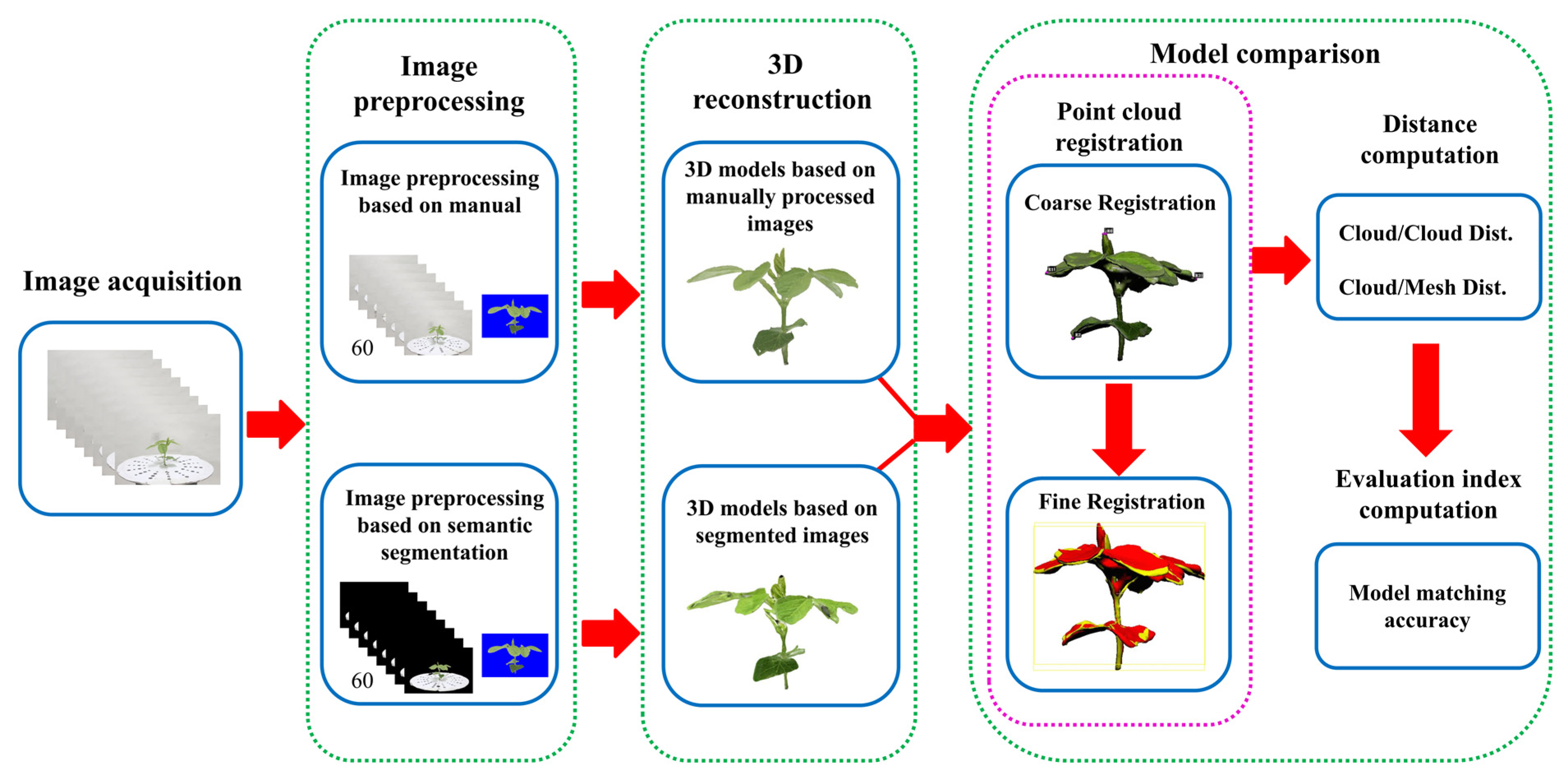
2.1. Overview of Method

The research methodology of the present study consists of four main parts:

• Image data acquisition;
• Manual image preprocessing and semantic-segmentation-based image preprocessing;
• Model establishment using both methods;
• Model accuracy comparison (coarse point cloud registration, fine point cloud registration, distance calculation and model matching accuracy calculation).

An overview of the proposed method can be seen in Figure 1.

2.2. Experimental Material

The soybean experiment was conducted at the soybean experimental base of Northeast Agricultural University, Harbin, China, located at 44°04′ N, 125°42′ E. Five varieties of soybeans, DN 251, DN 252, DN 253, HN 48 and HN 51, were selected for the experiment. The experiment was conducted in black soil using the container planting method. The soybean materials were planted in resin barrels with a height of 31 cm and a diameter of 27.5 cm. The bottoms of the resin barrels had multiple drainage holes to facilitate root respiration. In order to approximate the growth of the plants in the pot and the growth of the plants in the field, the experiment materials were placed in the field environment approximately 20 cm underground. An indoor 3D reconstruction experiment platform was established, utilizing MVS technology as the foundational technology. Soybean plants at different growth stages were moved indoors for 3D reconstruction image acquisition.

2.3. Image Acquisition

Multi-angle image acquisition was the basis for the MVS technology in the present study. The information required for 3D modeling of soybean plants was obtained from multi-angle image acquisition. When capturing multi-angle images, the object or camera needed to be rotated to obtain images from different perspectives and pitch angles of the target object. The tools used for plant image acquisition in the present study included the following: (1) a photo booth, (2) a Canon EOS600D DSLR camera (Canon (China) Co., Ltd., Beijing, China) and camera bracket, (3) a turntable, (4) a calibration mat, (5) a white-light-absorbing background cloth and (6) lighting. The process of image acquisition for a soybean plant involved the following:

• First, the reconstruction target was placed on the turntable in the photo booth, and a circular calibration mat was placed at the base of the plant. The position and brightness of the lighting were adjusted to ensure a good environment for target reconstruction.
• Second, the camera was placed approximately 90 cm away from the reconstruction target and the camera height was adjusted to the lowest position.
• Third, circular photography was used and the turntable was manually rotated every 24° (determined by the black dot on the calibration mat) to capture 15 images per revolution.
• Finally, the camera height was adjusted three times from low to high to obtain a sequence of 60 images of soybean plant morphology.
• Figure 2 shows the soybean image acquisition platform and image acquisition method flowchart. Such a method can effectively alleviate the problem of mutual occlusion between soybean leaves. Additionally, in this study, MVS technology was used to capture images of soybean plants during the vegetative stage.

2.4. Image Preprocessing

2.4.1. Manual-Based Image Preprocessing

In order to eliminate noise from each set of soybean plant images (60 images), filtering and smoothing methods were used. Through the analysis of the actual soybean plant morphology sequence images, the majority of image pollution noise was determined to be Gaussian white noise. Thus, a threshold denoising method based on wavelet transform was selected to denoise each soybean plant morphology sequence image [17]. The images were then segmented using the standard color key technique [18]. Manual refinement masking was applied to remove irrelevant backgrounds and calibration pad areas from all images, resulting in 60 images that only retained complete soybean plant images. These images served as the data foundation for building a soybean 3D model based on manual preprocessing.

2.4.2. Image Preprocessing Based on Semantic Segmentation

Image segmentation is a pivotal task in the domain of computer vision, alongside classification and detection. The primary objective of this task is to partition an image into multiple coherent segments based on the underlying content present within the image. In the present research, LabelMe was used to annotate 500 images of soybean plants during the vegetative period. The soybean plants and the calibration pad were labeled as a whole and marked as “soybean”. The training set and testing set were divided in an 8:2 ratio. A dataset was created for semantic segmentation, and the dataset link is https://pan.baidu.com/s/13qpZsOl3bgmAgua2D441UQ (accessed on 4 August 2023). Extract code: dr2v.

Four deep-learning-based semantic segmentation models were selected as follows: DeepLabv3+ [19], Unet [20], PSPnet [21] and HRnet [22]. These models were used to separate the soybean plants and the calibration pad from the background. Figure 3 shows the network architectures of these four semantic segmentation models.

• DeepLabv3+. The DeepLab series of networks are models specifically designed for semantic segmentation and were proposed by Liang Chieh Chen [23] and the Google team. The encoder–decoder structure used in DeepLabv3+ is innovative. The encoder is mainly responsible for encoding rich contextual information, while the concise and efficient decoder is used to recover the boundaries of the detected objects. Further, the network utilizes Atrous convolutions to achieve feature extraction at any resolution, enabling a more optimal balance between detection speed and accuracy.
• Unet. Unet is a model that was proposed by Olaf Ronneberger et al. [24] in 2015 for solving medical image segmentation problems. Unet consists of a contracting path, which serves as a feature extraction network to extract abstract features from the image, and an expansive path, which performs feature fusion operations. Compared with other segmentation models, Unet has a simple structure and larger operation space.
• PSPnet. The Pyramid Scene Parsing Network (PSPnet), proposed by Hengshuang Zhao et al. [25], is a model designed to address scene analysis problems. PSPnet is a neural network that uses the Pyramid Pooling Module to fuse features at four different scales. These pooling layers pool the original feature map, generating feature maps at various levels. Subsequently, convolution and upsampling operations are applied to restore the feature maps to their original size. By combining local and global information, PSPnet improves the reliability of final predictions.
• HRnet. The HRnet model, proposed by Ke Sun et al. [26], is composed of multiple parallel subnetworks with decreasing resolutions, which exchange information through multi-scale fusion. The depth of the network is represented horizontally, while the change in feature map (resolution) size is represented vertically. Such an approach allows for the preservation of high-resolution features throughout the process, without the need for resolution upsampling. As a result, the predicted keypoint heatmaps have a more accurate spatial distribution.

In the present study, removal of irrelevant backgrounds and calibration pad areas was performed on all 60 segmented images obtained from the semantic segmentation prediction, which served as the data foundation for constructing a 3D soybean model based on segmentation images.

2.5. 3D Reconstruction

In the present study, the “SAVANT” [27] method was utilized to establish a 3D model of soybean plants based on images obtained from three different noise removal preprocessing methods. SAVANT is a new algorithm for efficiently computing the boundary representation of the visual hull. Figure 4 illustrates the basic process of three-dimensional reconstruction. The specific process is as follows:

• First, the shooting direction of the corresponding image is determined by the position of different points on the calibration pad, and the multi-angle image obtained is calibrated.
• Second, under the conditions of two different image preprocessing methods, images with purified backgrounds were obtained, retaining only the complete information about the soybean plants.
• Third, based on the partial information about the target object from multi-angle images, several polygonal approximations of the contours were obtained. Each approximation was assigned a number, and three vertices were calculated from the polygonal contour. The information about each vertex was recorded.
• Fourth, by using a triangular grid, the complete surface was divided to outline surface details. At this point, the basic skeleton of the soybean three-dimensional plant model was generated;
• Finally, texture mapping was performed. Using the orientation information extracted from the three-dimensional surface contour model of the soybean plant and incorporating orientation details from various multi-angle images, texture mapping was employed to enhance the visualization features of the surface. The aim of such a process is to provide a more comprehensive depiction of the actual object’s characteristics.

2.6. Model Comparison

The open-source software CloudCompare v2.6.3 was used to complete the comparison between 3D models created based on manually preprocessed images and 3D models created based on segmented images. Figure 5 shows the main workflow of such an approach. Firstly, the alignment of the two entities was achieved by importing the comparison model and the reference model (where the reference model has a larger point cloud). The Align (point pairs picking) tool was used to select at least three corresponding point pairs from both models for alignment. The preview results, which include the contribution of each point pair to the matching error, are observable. New points could be added to these two sets at any time to add more constraints and obtain more reliable results. The optimal scaling factor between the two point sets could be determined by adjusting the scale. After alignment, an initial rotation and translation matrix were obtained. Secondly, the Fine registration (ICP) tool was used to achieve precise alignment of the two models. During the iteration process, the registration error slowly decreased. The iteration could be stopped after reaching the maximum number of iterations or when the RMS difference between two iterations was below a given threshold, depending on the setting of the number of iterations parameter. Reducing the threshold value leads to a longer convergence time requirement; however, it results in a more precise outcome. Thirdly, the octree was used for fast localization of each element and for searching the nearest region or point. The distance was calculated by means of two methods: the distance between point clouds and the distance between point clouds and meshes. Finally, the model matching accuracy was calculated.

2.6.1. Point Cloud Registration

Point cloud registration refers to the process of finding the transformation relationship between two sets of 3D data points from different coordinate systems. The purpose of point cloud registration is to compare or merge point cloud models obtained under different conditions for the same object. In an ideal scenario with no errors, this can be represented by the following equation:

$$p_t=R\cdot q_s+t,$$

(1)

where p_t and q_s are corresponding points from the target and source point clouds, respectively (the points with the closest Euclidean distance), R represents the rotation matrix and t represents the translation vector.

Presently, point cloud registration can be divided into two stages: coarse registration and fine registration.

Coarse registration refers to the process of aligning point clouds when the relative pose between them is entirely unknown. The primary objective is to discover a rotation and translation transformation matrix that can approximately align the two point clouds. This allows the point cloud data to be transformed into a unified coordinate system, providing a good initial position for fine registration. In the present study, the RANSAC (Random Sample Consensus) algorithm [28,29] was employed for point cloud coarse registration. The algorithm can be summarized as follows:

• Select at least three corresponding point pairs. Randomly choose three non-collinear data points {q₁, q₂, q₃} from the source cloud Q, and select the corresponding point set {p₁, p₂, p₃} from the target cloud P.
• Calculate the rotation and translation matrix H using the least squares method for these two point sets.
• Transform the source cloud Q into a new three-dimensional point cloud dataset Q′ using the transformation matrix H. Compare Q′ with P and extract all points (inliers) of which the distance deviation is less than a given threshold k to form a consistent point cloud set S1’. Record the number of inliers.
• Set a threshold K and repeat the above process. After performing the operation K times, if a consistent point cloud set cannot be obtained, the model parameter estimation fails. If a consistent point cloud set is obtained, select the one with the maximum number of inliers. The corresponding rotation and translation matrix H at this point is the optimal model parameter.

The initial coarse registration aligns the source cloud Q and the target cloud P approximately, but in order to improve the accuracy of point cloud registration, fine registration needs to be performed. In the present study, fine registration of point clouds was implemented based on the Iterative Closest Point (ICP) algorithm [30]. The aim of the ICP algorithm is to minimize the difference between two clouds of points by finding the closest points in the two point clouds. The algorithm works as follows:

• Based on the approximate parameter values of R and t obtained from the coarse registration of the point cloud, the corresponding points are directly searched for by identifying the closest points in the two point clouds;
• The least squares method is used to construct an objective function and iteratively minimize the overall distance between the corresponding points until the termination condition is met (either the maximum number of iterations or the error is below a threshold). This ultimately allows for the rigid transformation matrix to be obtained.

The core of the ICP algorithm is to minimize an objective function, which is essentially the sum of the squared Euclidean distances between all corresponding points. The objective function can be described as

$${{\displaystyle E(R,t)=\frac{1}{n}{\displaystyle \sum _{i=1}^n‖p_t-(R\cdot q_s+t)‖}}}^2,$$

(2)

where E is the Euclidean norm, R is the rotation matrix, t is the translation vector, n is the number of point pairs between the two point clouds and p_t and q_s are a pair of corresponding points from the target cloud and source cloud, respectively. As such, the ICP problem can be described as finding the values of R and t that minimize E(R, t).

The ICP problem can be solved using linear algebra (SVD) with the following steps:

• Compute the centroids of the two sets of corresponding points;

$${\overline{p}}_t=\frac{1}{n}{\displaystyle \sum _{i=1}^n{p}_t},$$

(3)

$${\overline{q}}_s=\frac{1}{n}{\displaystyle \sum _{i=1}^n{q}_s},$$

(4)

• Obtain the point sets without centroids;

$$P^{\prime }=\left\{p_t-{\overline{p}}_t\right\}=\left\{p_t^{\prime }\right\},$$

(5)

$$Q^{\prime }=\left\{q_s-{\overline{q}}_s\right\}=\left\{q_s^{\prime }\right\},$$

(6)

• Calculate the 3 × 3 matrix H;

$$H=X{Y}^T,$$

(7)

where X and Y are the source and target point cloud matrices of the centroid removal, respectively, with sizes of 3xn.

• Perform SVD decomposition on H;

$$H=U{\mathsf{\Sigma }\mathrm{V}}^{\mathrm{T}},$$

(8)

where U is an m × m matrix, Σ is an m × n matrix with all elements as 0 except for the principal diagonal (representing singular values) and V is an n × n matrix.

• Calculate the optimal rotation matrix;

$$R=U{V}^T,$$

(9)

• Calculate the optimal translation vector.

$$t={\overline{p}}_t-R{\overline{q}}_s,$$

(10)

2.6.2. Distance Calculation

When comparing the similarity of two sets of models, distance is commonly used to quantify the degree of overlap, where a higher degree of overlap indicates a higher similarity. The default method for calculating the distance between two point clouds is the “nearest neighbor distance”. The simplest and most direct approach is to calculate the Euclidean distance between a point on one point cloud and the nearest point on the other point cloud. For two points p₁ (x_p, y_p, z_p) and q₁ (x_q, y_q, z_q) on the two point clouds, the Euclidean distance between the two points can be defined as

$$d(p_1,q_1)=\sqrt{{(x_p-x_q)}^2+{(y_p-y_q)}^2+{(z_p-z_q)}^2},$$

(11)

However, due to missing data in some point clouds, there may be significant errors between the measured distance and the true distance. As such, the distance from a point to the model’s mesh could be calculated. Such an approach is statistically more accurate and less dependent on cloud sampling. The calculation method is as follows:

Given that the plane equation of the closest triangle mesh Q₁ to the point p₁ (x, y, z) in the reference model is

$$Ax+By+Cz+D=0,$$

(12)

the distance from point p₁ (x, y, z) to the mesh Q₁ is

$$d(p_1,Q_1)=\frac{\left|Ax+By+Cz+D\right|}{\sqrt{A^2+B^2+C^2}},$$

(13)

2.7. Evaluation Index of Automatic Image Preprocessing and Model Effect

2.7.1. Semantic Segmentation

With the aim of overcoming the multi-semantic segmentation problem, four indicators of mean Intersection over Union (mIoU), mean Pixel Accuracy (mPA), Precision and Recall were used to comprehensively evaluate the performance of the model. The formulas of mIoU, mPA, Precision and Recall are as follows:

$$mIoU=\frac{1}{k+1}{\displaystyle \sum _{i=0}^k\frac{TP}{FN+FP+TP}},$$

(14)

$$MPA=\frac{1}{k+1}{\displaystyle \sum _{i=0}^k\frac{TP}{TP+FP}},$$

(15)

$$Precision=\frac{TP}{TP+FP},$$

(16)

$$Recall=\frac{TP}{TP+FN},$$

(17)

In the present study, the number of true positives, true negatives, false positives and false negatives for each class were denoted as TP, TN, FP and FN, respectively. Here, i represents the class and k + 1 represents the total number of target classes and one background class.

2.7.2. Point Cloud Registration

The root mean square error (RMSE) is commonly used as the termination criterion for point cloud matching iterations. The RMSE is calculated using the formula

$$RMSE=\sqrt{\frac{{\displaystyle \sum _{i=1}^n{(x_i-{\widehat{x}}_i)}^2}}{n}},$$

(18)

where n is the number of corresponding points, x_i is the Euclidean distance between corresponding points after registration and ${\widehat{x}}_{\mathrm{i}}$ is the ground truth Euclidean distance between corresponding points. In the ideal scenario, where the registration is perfect, the ground truth Euclidean distance would be 0. Therefore, in the present study, the RMS value was used as the indicator for terminating the point cloud matching iterations. The formula for the RMS value is

$$RMS=\sqrt{\frac{{\displaystyle \sum _{i=1}^n{x_i}^2}}{n}},$$

(19)

2.7.3. Distance between Models

After calculating the distances between points and between points and the mesh of the models being compared, the mean distance ($\overline{d}$) and the standard deviation ($\sigma$) were calculated to evaluate the similarity and stability of the models:

$$\overline{d}=\frac{1}{N}{\displaystyle \sum _{i=1}^N{d}_i},$$

(20)

$$\sigma =\sqrt{\frac{{\displaystyle \sum _{i=1}^N{(d_i-\overline{d})}^2}}{N}},$$

(21)

where N is the number of points in the comparison model and d_i represents the distance between points or the distance between points and the mesh.

2.7.4. Model Matching Accuracy

To evaluate the accuracy of the soybean plant 3D model established based on segmented images, the model matching accuracy (α) was introduced as the evaluation metric. If group i points match, then αi is 1, and if group i points do not match, then αi is 0. Specifically, this is defined as

$$m=min\{N,M\},$$

(22)

$$if\hspace{0.33em}d(p_i,q_i)\hspace{0.33em}or\hspace{0.33em}d(p_i,Q_i)\ge C_0,\hspace{0.33em}then\hspace{0.33em}{\alpha }_i=0,$$

(23)

$$if\hspace{0.33em}d(p_i,q_i)\hspace{0.33em}or\hspace{0.33em}d(p_i,Q_i)<C_0,\hspace{0.33em}then\hspace{0.33em}{\alpha }_i=1,$$

(24)

$$\alpha =\frac{1}{m}{\displaystyle \sum _{i=1}^m{\alpha }_i},$$

(25)

where P and Q are the reference point cloud and the comparison point cloud, p_i and q_i are a set of matching points in P and Q, d (p_i, q_i) is the Euclidean distance between two matching points and d (p_i, Q_i) is the Euclidean distance to the nearest mesh. N and M represent the point cloud quantities of P and Q, respectively, and m represents the point cloud with the smaller number of points between the two point clouds. According to experience, the selection of C₀ is generally selected according to the gradient of 2, 3 and 4. The selection of different C₀ values will produce different evaluation results.

3. Results

3.1. Semantic Segmentation

Four deep learning semantic segmentation models were used in the present study, namely DeepLabv3+, Unet, PSPnet and HRnet, to train on 500 well-labeled soybean images. The training was conducted with a batch size of four and 200 epochs. Figure 6 displays the training loss and train mIoU variation curves during the training process of the four models. After 200 epochs, both the training and validation loss reached a stable state, and the train mIoU remained stable after reaching its peak, indicating good training performance.

The DeepLabv3+, Unet, PSPnet and HRnet models were tested on a test set, and all four models demonstrated good segmentation performance. Figure A1 in Appendix A presents the confusion matrix of the results obtained from the four models. The performance of the different models was compared using four evaluation metrics: mIoU, mPA, mPrecision, and mRecall.

Table 1. Comparison of test results of DeepLabv3+, Unet, PSPnet and HRnet.

	mIoU	mPA	mPrecision	mRecall
DeepLabv3+	0.9887	0.9948	0.9938	0.9948
Unet	0.9919	0.9953	0.9965	0.9953
PSPnet	0.9624	0.9794	0.9819	0.9794
HRnet	0.9883	0.9943	0.9939	0.9943

and Figure A2 in Appendix A provide a comparison of the test results for the DeepLabv3+, Unet, PSPnet and HRnet models. The comparison results indicate that all four semantic segmentation models were capable of effectively segmenting soybeans and calibration pads from the background. Among the models, the Unet model demonstrated the optimal performance.

3.2. Model Distance Comparison

Three-dimensional reconstruction of soybean plant images obtained using two image preprocessing methods was conducted, and the constructed model data were linked as follows: https://pan.baidu.com/s/1UIBAts1dbjIiLvBv6YVpPA (accessed on 4 August 2023). Extract code: 65xf.

Align and Fine registration operations were performed on the comparison model and reference model.

Table 2. The final RMS before the end of the two process iterations.

Variety	Period	RMS (Align)	RMS (Fine Registration)
DN251	V1	1.95626	1.19971
	V2	2.09126	1.35077
	V3	4.58306	2.58519
	V4	4.46901	2.65409
	V5	3.18775	2.87697
DN252	V1	2.63826	1.48934
	V2	7.80912	3.23065
	V3	1.80913	2.89284
	V4	1.69937	5.33
	V5	6.16305	13.713
DN253	V1	0.738292	1.02404
	V2	1.27929	1.06568
	V3	1.6837	2.40657
	V4	1.91016	3.61526
	V5	5.73199	4.7968
HN48	V1	1.26657	0.909976
	V2	1.4727	1.18007
	V3	1.04926	1.63755
	V4	0.0957965	4.35126
	V5	6.02313	11.6697
HN51	V1	1.30144	0.569594
	V2	2.33492	0.940522
	V3	0.529973	1.44398
	V4	1.44441	1.85106
	V5	2.88033	5.97911

shows the final RMS before the end of the two process iterations. The iteration was stopped when the error (RMS) between the two iterations was below a given threshold.

Using two methods, Cloud to Cloud Dist. and Cloud to Mesh Dist., the distance between the comparison model and the reference model was calculated and compared. Model distance is a measure of the magnitude of error between models and serves as the basis for calculating model matching data. Figure 7 displays a bar chart illustrating the approximate distance between the comparison model and the reference model at various stages of DN251 soybean plants using the two methods. Additionally, the soybean plants of the other varieties are presented in the Supplementary Materials.

Table 3. The average distance and standard deviation between the comparison model and the reference model using the two methods.

Variety	Period	Cloud/Cloud Dist.		Cloud/Mesh Dist.
		Mean Dist.	Std Deviation	Mean Dist.	Std Deviation
DN251	V1	1.145612	0.900235	1.130519	0.911150
	V2	1.158162	1.030425	1.076919	1.069205
	V3	2.262815	1.887179	2.183569	1.938041
	V4	2.088518	1.881370	2.000282	1.930785
	V5	1.998276	1.548111	1.836738	1.619279
DN252	V1	1.026802	0.780924	0.966741	0.809431
	V2	2.971597	2.662797	2.926895	2.695811
	V3	2.404866	2.627851	2.391443	2.635576
	V4	4.052322	4.064967	3.960502	4.120001
	V5	11.601336	11.490972	11.523714	11.549747
DN253	V1	0.674987	0.562897	0.649014	0.576336
	V2	1.034015	0.763250	0.952814	0.804699
	V3	1.903690	1.582029	1.831233	1.623182
	V4	2.693205	2.117353	2.610196	2.164421
	V5	3.555374	4.216107	3.449008	4.265732
HN48	V1	0.776107	0.563027	0.756657	0.575204
	V2	1.033295	0.750766	0.959216	0.783948
	V3	1.223996	0.939598	1.175414	0.966041
	V4	3.412442	3.460865	3.362041	3.494898
	V5	7.974715	8.950619	7.871541	9.018435
HN51	V1	0.493069	0.353827	0.468149	0.365837
	V2	0.765773	0.473434	0.697317	0.506449
	V3	1.233639	0.917520	1.170139	0.948327
	V4	1.647804	1.188333	1.571436	1.227389
	V5	4.725530	4.344229	4.691150	4.369667

presents the average distance and standard deviation between the comparison model and the reference model using the two methods. By comparing the results, the following conclusions could be drawn:

• First, for soybean plants of the same variety, the distance between the plant models increased with the stage of growth;
• Second, for soybean plants at the same stage of growth, the distance between models of different varieties remained approximately the same;
• Third, the time required to establish soybean plant models based on segmented images was significantly shorter than the time needed for models based on manual image preprocessing;
• Such findings indicate that in image-based crop 3D reconstruction, semantic segmentation can effectively improve the difficulties and long reconstruction time associated with preprocessing images of soybean plants of different varieties at different stages, greatly enhance the robustness to noisy input and ensure the accuracy of the models.

3.3. Model Matching Accuracy

Based on the approximate distance between the comparative model and the reference model, the matching accuracy between different models was calculated. The model matching accuracy was used to measure the similarity between the two models.

Table 4. Model matching degree α₂ when C₀ is the second digit.

	V1		V2		V3		V4		V5
	Cloud/Cloud	Cloud/Mesh	Cloud/Cloud	Cloud/Mesh	Cloud/Cloud	Cloud/Mesh	Cloud/Cloud	Cloud/Mesh	Cloud/Cloud	Cloud/Mesh
DN251	0.7525	0.7516	0.8574	0.8564	0.6908	0.6894	0.7745	0.7750	0.8654	0.8659
DN252	0.7771	0.7804	0.6658	0.6620	0.8445	0.8441	0.8396	0.8387	0.6958	0.6951
DN253	0.8754	0.8741	0.6842	0.6893	0.8438	0.8417	0.7312	0.7336	0.8736	0.8734
HN48	0.5698	0.5747	0.6173	0.6222	0.6751	0.6808	0.7967	0.7960	0.8303	0.8298
HN51	0.6710	0.6793	0.6112	0.6285	0.6933	0.6988	0.6467	0.6553	0.7423	0.7414

,

Table 5. Model matching degree α₃ when C₀ is the third digit.

	V1		V2		V3		V4		V5
	Cloud/Cloud	Cloud/Mesh	Cloud/Cloud	Cloud/Mesh	Cloud/Cloud	Cloud/Mesh	Cloud/Cloud	Cloud/Mesh	Cloud/Cloud	Cloud/Mesh
DN251	0.9082	0.9079	0.9295	0.9293	0.8369	0.8360	0.8985	0.8980	0.9513	0.9512
DN252	0.9202	0.9215	0.8262	0.8264	0.9311	0.9311	0.9348	0.9341	0.7918	0.7915
DN253	0.9587	0.9584	0.8257	0.8218	0.9471	0.9463	0.8941	0.8947	0.9196	0.9196
HN48	0.7526	0.7534	0.7865	0.7871	0.8434	0.8454	0.9093	0.9090	0.8972	0.8969
HN51	0.8543	0.8584	0.8241	0.8274	0.8624	0.8645	0.8376	0.8400	0.8503	0.8498

and

Table 6. Model matching degree α₄ when C₀ is the fourth digit.

	V1		V2		V3		V4		V5
	Cloud/Cloud	Cloud/Mesh	Cloud/Cloud	Cloud/Mesh	Cloud/Cloud	Cloud/Mesh	Cloud/Cloud	Cloud/Mesh	Cloud/Cloud	Cloud/Mesh
DN251	0.9767	0.9767	0.9679	0.9679	0.9241	0.9225	0.9510	0.9508	0.9811	0.9812
DN252	0.9680	0.9681	0.8912	0.8906	0.9667	0.9667	0.9665	0.9661	0.8736	0.8736
DN253	0.9853	0.9852	0.9189	0.9132	0.9847	0.9843	0.9529	0.9534	0.9388	0.9385
HN48	0.8754	0.8760	0.8886	0.8886	0.9273	0.9283	0.9544	0.9541	0.9331	0.9330
HN51	0.9485	0.9503	0.9407	0.9389	0.9334	0.9342	0.9332	0.9338	0.9219	0.9218

show the results of the model matching accuracy with threshold C₀ set at the second digit, third digit and fourth digit, respectively. Among them, C₀ is the second digit, indicating that the distance between the models is about 1 pixel; C₀ is the third digit, indicating that the distance between the models is about 2 pixels; C₀ is the fourth digit, indicating that the distance between the models is about 3 pixels.

By analyzing the matching accuracy between models at different thresholds, a conclusion could be drawn that the model based on manually preprocessed images matched well with the model based on segmented images. Figure 8 shows the schematic of the point cloud model of HN51 soybean plants at different stages using both methods. The findings indicate that semantic segmentation can effectively improve the difficulties in preprocessing images of soybean plants of various varieties and stages, as well as reduce reconstruction time. Such a method can also greatly enhance the robustness to noisy input and ensure the accuracy of the model. Through semantic segmentation, an important foundation is provided for efficient and automated image preprocessing in the 3D reconstruction of soybean plants at the vegetative stage.

4. Discussion

Traditional image preprocessing methods are typically carried out manually, which can be tedious and time-consuming. To enhance the efficiency of image preprocessing and alleviate the difficulty of noise reduction in manual preprocessing, the use of semantic segmentation was proposed for automated preprocessing of 3D reconstruction images of soybean plants. The results of comparative experiments reveal that semantic segmentation can effectively alleviate the issues in image preprocessing and can be applied in image-based 3D reconstruction tasks. During the experimental process, there were three main factors that influenced the reconstruction model.

The first factor is the accuracy of semantic segmentation. The aim of semantic segmentation is to simplify or modify the representation of an image, making it easier to analyze. Attari et al. [31] proposed a hybrid noise removal and binarization algorithm to separate foreground and background and obtain plant images, which aids in plant image segmentation. Rzanny et al. [32] developed a semi-automatic method based on the GrabCut algorithm to efficiently segment images of wild flowering plants. GrabCut, based on iterative graph cuts, is considered an accurate and effective method for interactive image segmentation. Milioto et al. [33] addressed the semantic segmentation problem in crop fields using only RGB data, focusing on distinguishing sugar beets, weeds and the background. A CNN-based method was established that leverages pre-existing vegetation indices to achieve real-time classification. In the present study, semantic segmentation was applied to 3D reconstruction image preprocessing, and a dataset of 500 soybean plant images at the vegetative stage was selected for semantic segmentation. This growth stage of soybean plants is characterized by regular morphology, simple growth patterns, short internode spacing, thick stems and thick leaves, which significantly alleviates the difficulty of data annotation and manual image preprocessing tasks. This was a significant factor in the success of the experiments. The segmented images obtained from semantic segmentation were used for the 3D reconstruction of soybean plant models. The analysis of the data results shows that the method can ensure the accuracy of the reconstructed models, reduce image preprocessing time, and improve work efficiency. In future research, the semantic segmentation models will be continuously refined to improve the segmentation accuracy and explore the efficiency of semantic segmentation methods in automating preprocessing tasks for soybean plant images throughout the entire growth cycle. Moreover, an investigation will be conducted into the role of semantic segmentation methods in the construction of 3D models for other crops.

The second factor is the complexity of soybean plants at different growth stages. The growth periods of soybean cultivars can vary significantly across different ecological regions, particularly in China, where a highly intricate soybean cropping system exists [34]. As the growth of soybean plants during the growth period continues, it becomes increasingly complex, which becomes a significant factor that affects the accuracy of the model. In the present study, soybean plants in five stages of the vegetative period were reconstructed, and the experimental comparison results reveal that as the growth period increased, the distance between the comparative model and the reference model became larger. At the same time, although the overall outlines of the models were roughly similar, there were still certain differences in the construction of local organs, especially in terms of the leaf shape. Figure 9 shows a schematic diagram of the point cloud reconstruction models of the same variety at different stages using two methods. The figure depicts the similarity of the outlines and the local differences between the two models. This phenomenon is strongly associated with the growth period of soybean plants.

The third factor is the differences between different varieties of soybean plants. The mechanisms of soybean growth and development need to be understood. Different types of soybeans can also affect the timing of flowering or podding stages in plants [35]. The differences in the growth process of soybean plants of different varieties during the same period could be observed through 3D reconstruction models. Further, the calculation results show that, during the same period, the soybean varieties DN251, DN253 and HN51 exhibited a better model fit, followed by DN252 and HN48. However, in the later stages, different soybean varieties also exhibited larger model distances, for instance, the DN252 soybean plant at the V5 stage and the HN48 soybean plant at the V5 stage. Figure 10 shows the point cloud reconstruction models of the DN252 soybean plant and the HN48 soybean plant at the V5 stage using two different methods. According to the figure, the differences in soybean plant varieties can evidently affect the reconstruction accuracy based on segmented image models.

5. Conclusions

In an effort to mitigate the challenges of image preprocessing, enhance the speed of 3D reconstruction for soybean plants and ensure the accuracy of the reconstruction model, four semantic segmentation networks were employed in the present study: DeepLabv3+, Unet, PSPnet and HRnet. The training dataset comprised 500 images of soybean plants in the vegetative stage. Among the models, the Unet network exhibited the optimal testing performance, with values of 0.9919, 0.9953, 0.9965 and 0.9953 for mIoU, mPA, mPrecision and mRecall, respectively. Subsequently, 3D models of soybean plants were established based on segmented images and manually preprocessed images, respectively, for comparative experiments. Through point cloud matching, distance calculation and model matching accuracy calculation, it was found that in image-based crop 3D reconstruction, semantic segmentation can effectively improve the difficulty of image preprocessing and the long reconstruction time while ensuring the accuracy of the model, greatly improving the robustness to noisy inputs. Semantic segmentation provides a vital foundation for efficient and automated image preprocessing for 3D reconstruction of soybean plants in the vegetative stage. In the future, we will apply semantic segmentation technology to the construction of three-dimensional model of soybean plants during the whole growth period, and continue to explore the influence of semantic segmentation on image preprocessing of different soybean plants and other crops.

References

1. Guan, H.; Liu, M.; Ma, X.; Yu, S. Three-Dimensional Reconstruction of Soybean Canopies Using Multisource Imaging for Phenotyping Analysis. Remote Sens. 2018, 10, 1206. [Google Scholar] [CrossRef]
2. Favre, P.; Gueritaine, G.; Andrieu, B.; Boumaza, R.; Demotes-Mainard, S.; Fournier, C.; Galopin, G.; Huche-Thelier, L.; Morel-Chevillet, P.; Guérin, V. Modelling the architectural growth and development of rosebush using L-Systems. In Proceedings of the Growth Phenotyping and Imaging in Plants, Montpellier, France, 17–19 July 2007. [Google Scholar]
3. Turgut, K.; Dutagaci, H.; Galopin, G.; Rousseau, D. Segmentation of structural parts of rosebush plants with 3D point-based deep learning methods. Plant Methods 2022, 18, 20. [Google Scholar] [CrossRef]
4. Zhu, R.; Sun, K.; Yan, Z.; Yan, X.; Yu, J.; Shi, J.; Hu, Z.; Jiang, H.; Xin, D.; Zhang, Z.; et al. Analysing the phenotype development of soybean plants using low-cost 3D reconstruction. Sci. Rep. 2020, 10, 7055. [Google Scholar] [CrossRef]
5. Martinez-Guanter, J.; Ribeiro, Á.; Peteinatos, G.G.; Pérez-Ruiz, M.; Gerhards, R.; Bengochea-Guevara, J.M.; Machleb, J.; Andújar, D. Low-Cost Three-Dimensional Modeling of Crop Plants. Sensors 2019, 19, 2883. [Google Scholar] [CrossRef]
6. Sun, Y.; Zhang, Z.; Sun, K.; Li, S.; Yu, J.; Miao, L.; Zhang, Z.; Li, Y.; Zhao, H.; Hu, Z.; et al. Soybean-MVS: Annotated Three-Dimensional Model Dataset of Whole Growth Period Soybeans for 3D Plant Organ Segmentation. Agriculture 2023, 13, 1321. [Google Scholar] [CrossRef]
7. Xiao, B.; Wu, S.; Guo, X.; Wen, W. A 3D Canopy Reconstruction and Phenotype Analysis Method for Wheat. In Proceedings of the 11th International Conference on Computer and Computing Technologies in Agriculture (CCTA), Jilin, China, 12–15 August 2017; pp. 244–252. [Google Scholar]
8. Bietresato, M.; Carabin, G.; Vidoni, R.; Gasparetto, A.; Mazzetto, F. Evaluation of a LiDAR-based 3D-stereoscopic vision system for crop-monitoring applications. Comput. Electron. Agric. 2016, 124, 1–13. [Google Scholar] [CrossRef]
9. Wu, J.; Xue, X.; Zhang, S.; Qin, W.; Chen, C.; Sun, T. Plant 3D reconstruction based on LiDAR and multi-view sequence images. Int. J. Precis. Agric. Aviat. 2018, 1, 37–43. [Google Scholar] [CrossRef]
10. Pan, Y.; Han, Y.; Wang, L.; Chen, J.; Meng, H.; Wang, G.; Zhang, Z.; Wang, S. 3d reconstruction of ground crops based on airborne lidar technology—Sciencedirect. IFAC-PapersOnLine 2019, 52, 35–40. [Google Scholar] [CrossRef]
11. Wu, S.; Wen, W.; Wang, Y.; Fan, J.; Wang, C.; Gou, W.; Guo, X. MVS-Pheno: A Portable and Low-Cost Phenotyping Platform for Maize Shoots Using Multiview Stereo 3D Reconstruction. Plant Phenomics 2020, 2020, 1848437. [Google Scholar] [CrossRef]
12. Li, Y.; Liu, J.; Zhang, B.; Wang, Y.; Yao, J.; Zhang, X.; Fan, B.; Li, X.; Hai, Y.; Fan, X. Three-dimensional reconstruction and phenotype measurement of maize seedlings based on multi-view image sequences. Front Plant Sci. 2022, 13, 974339. [Google Scholar] [CrossRef]
13. Song, P.; Li, Z.; Yang, M.; Shao, Y.; Pu, Z.; Yang, W.; Zhai, R. Dynamic detection of three-dimensional crop phenotypes based on a consumer-grade RGB-D camera. Front Plant Sci. 2023, 14, 1097725. [Google Scholar] [CrossRef]
14. Zhu, T.; Ma, X.; Guan, H.; Wu, X.; Wang, F.; Yang, C.; Jiang, Q. A calculation method of phenotypic traits based on three-dimensional reconstruction of tomato canopy. Comput. Electron. Agric. 2023, 204, 107515. [Google Scholar] [CrossRef]
15. Liu, Y.; Yuan, H.; Zhao, X.; Fan, C.; Cheng, M. Fast reconstruction method of three-dimension model based on dual RGB-D cameras for peanut plant. Plant Methods 2023, 19, 17. [Google Scholar] [CrossRef]
16. Minh, T.N.; Sinn, M.; Lam, H.T.; Wistuba, M. Automated image data preprocessing with deep reinforcement learning. arXiv 2018, arXiv:1806.05886. [Google Scholar]
17. Chang, S.G.; Yu, B. Adaptive wavelet thresholding for image denoising and compression. IEEE Trans. Image Process. 2000, 9, 1532. [Google Scholar] [CrossRef]
18. Smith, A.R.; Blinn, J.F. Blue screen matting. In Proceedings of the 23rd Annual Conference on Computer Graphics and Interactive Techniques, New Orleans, LA, USA, 4–9 August 1996; Association for Computing Machinery: New York, NY, USA, 1996; pp. 259–268. [Google Scholar]
19. DeepLabv3+. Available online: https://github.com/18545155636/Deeplabv3.git (accessed on 4 August 2023).
20. Unet. Available online: https://github.com/18545155636/Unet.git (accessed on 4 August 2023).
21. PSPnet. Available online: https://github.com/18545155636/PSPnet.git (accessed on 4 August 2023).
22. HRnet. Available online: https://github.com/18545155636/HRnet.git (accessed on 4 August 2023).
23. Chen, L.C.; Zhu, Y.; Papandreou, G.; Schroff, F.; Adam, H. Encoder-Decoder with Atrous Separable Convolution for Semantic Image Segmentation. In Proceedings of the European Conference on Computer Vision–ECCV 2018, Munich, Germany, 8–14 September 2018; Springer: Berlin/Heidelberg, Germany, 2018. [Google Scholar]
24. Ronneberger, O.; Fischer, P.; Brox, T. U-Net: Convolutional Networks for Biomedical Image Segmentation. arXiv 2015, arXiv:1505.04597. [Google Scholar]
25. Zhao, H.; Shi, J.; Qi, X.; Wang, X.; Jia, J. Pyramid Scene Parsing Network. In Proceedings of the 2017 IEEE Conference on Computer Vision and Pattern Recognition (CVPR), Honolulu, HI, USA, 21–26 July 2017; pp. 6230–6239. [Google Scholar]
26. Sun, K.; Xiao, B.; Liu, D.; Wang, J. Deep High-Resolution Representation Learning for Human Pose Estimation. In Proceedings of the 2019 IEEE/CVF Conference on Computer Vision and Pattern Recognition (CVPR), Long Beach, CA, USA, 15–20 June 2019; pp. 5686–5696. [Google Scholar]
27. Baumberg, A.; Lyons, A.; Taylor, R. 3d s.o.m.—A commercial software solution to 3d scanning. Graph. Models 2005, 67, 476–495. [Google Scholar] [CrossRef]
28. Fischler, M.A.; Bolles, R.C. Random sample consensus: A paradigm for model fitting with applications to image analysis and automated cartography. Commun. ACM 1981, 24, 381–395. [Google Scholar] [CrossRef]
29. Chen, C.S.; Hung, Y.P.; Cheng, J.B. Ransac-based darces: A new approach to fast automatic registration of partially overlapping range images. IEEE Trans. Pattern Anal. Mach. Intell. 2002, 21, 1229–1234. [Google Scholar] [CrossRef]
30. Besl, P.J.; McKay, N.D. A Method for Registration of 3-D Shapes. IEEE Trans. Pattern Anal. Mach. Intell. 1992, 14, 239–256. [Google Scholar] [CrossRef]
31. Attari, H.; Ghafari-Beranghar, A. An Efficient Preprocessing Algorithm for Image-based Plant Phenotyping. Preprints 2018, 20180402092018. [Google Scholar] [CrossRef]
32. Rzanny, M.; Seeland, M.; Waldchen, J.; Mader, P. Acquiring and preprocessing leaf images for automated plant identification: Understanding the tradeoff between effort and information gain. Plant Methods 2017, 13, 97. [Google Scholar] [CrossRef]
33. Milioto, A.; Lottes, P.; Stachniss, C. Real-time Semantic Segmentation of Crop and Weed for Precision Agriculture Robots Leveraging Background Knowledge in CNNs. In Proceedings of the 2018 IEEE International Conference on Robotics and Automation (ICRA), Brisbane, QLD, Australia, 21–25 May 2018; pp. 2229–2235. [Google Scholar]
34. Wang, X.-B.; Liu, Z.-X.; Yang, C.-Y.; Xu, R.; Lu, W.-G.; Zhang, L.-F.; Wang, Q.; Wei, S.-H.; Yang, C.-M.; Wang, H.-C.; et al. Stability of growth periods traits for soybean cultivars across multiple locations. J. Integr. Agric. 2016, 15, 963–972. [Google Scholar] [CrossRef]
35. Schapaugh, W.T. Variety Selection. In Soybean Production Handbook; Publication C449; K-State Research and Extension: Manhattan, KS, USA, 2016. [Google Scholar]
Figure 1. An overview of the proposed method.
Agronomy 13 02388 g001
Figure 2. Soybean 3D reconstruction image acquisition. (a) Soybean image acquisition platform; (b) image acquisition method flowchart.
Agronomy 13 02388 g002
Figure 3. Semantic segmentation model architecture. (a) DeepLabv3+; (b) Unet; (c) PSPnet; (d) HRNet.
Agronomy 13 02388 g003aAgronomy 13 02388 g003b
Figure 4. The process of 3D reconstruction of soybean plants.
Agronomy 13 02388 g004
Figure 5. The process of model comparison.
Agronomy 13 02388 g005
Figure 6. The training loss and train mIoU variation curves during the training process of the four models. (a) DeepLabv3+; (b) Unet; (c) PSPnet; (d) HRNet.
Agronomy 13 02388 g006aAgronomy 13 02388 g006b
Figure 7. Histogram of approximate distance between comparison model and reference model of DN251 soybean plant at different stages. (a) V1 stage; (b) V2 stage; (c) V3 stage; (d) V4 stage; (e) V5 stage. (Left is Cloud/Cloud Dist. Right is Cloud/Mesh Dist.).
Agronomy 13 02388 g007aAgronomy 13 02388 g007b
Figure 8. The schematic of the point cloud model of HN51 soybean plants at different stages using both methods. (a) V1 stage; (b) V2 stage; (c) V3 stage; (d) V4 stage; (e) V5 stage. (Left is soybean 3D point cloud models based on segmentation image. Right is soybean 3D point cloud models based on manually preprocessed image).
Agronomy 13 02388 g008aAgronomy 13 02388 g008b
Figure 9. Local schematic diagram of HN 51 soybean plant point cloud model in different stages using the two methods. (a) V1 stage; (b) V2 stage; (c) V3 stage; (d) V4 stage; (e) V5 stage. (Left is soybean 3D point cloud models based on segmentation image. Right is soybean 3D point cloud models based on manually preprocessed image).
Agronomy 13 02388 g009aAgronomy 13 02388 g009b
Figure 10. Using the two methods, the point cloud diagram of DN 252 soybean plants in V5 and HN 48 soybean plants in V5. (a) DN 252 soybean plant at V5 stage; (b) HN 48 soybean plant at V5 stage.
Agronomy 13 02388 g010aAgronomy 13 02388 g010b