A Sensor-Based Decision Model for Precision Weed Harrowing

Abstract

Weed harrowing is commonly used to manage weeds in organic farming but is also applied in conventional farming to replace herbicides. Due to its whole-field application, weed harrowing after crop emergence has relatively poor selectivity and may cause crop damage. Weediness generally varies within a field. Therefore, there is a potential to improve the selectivity and consider the within-field variation in weediness. This paper describes a decision model for precision post-emergence weed harrowing in cereals based on experimental data in spring barley and nonlinear regression analysis. The model predicts the optimal weed harrowing intensity in terms of the tine angle of the harrow for a given weediness (in terms of percentage weed cover), a given draft force of tines, and the biological weed damage threshold (in terms of percentage weed cover). Weed cover was measured with near-ground RGB images analyzed with a machine vision algorithm based on deep learning techniques. The draft force of tines was estimated with an electronic load cell. The proposed model is the first that uses a weed damage threshold in addition to site-specific values of weed cover and soil hardness to predict the site-specific optimal weed harrow tine angle. Future field trials should validate the suggested model.

1. Introduction

The massive use of herbicides has resulted in increasing problems with herbicide-resistant weeds [1] and an unintentionally negative impact on living organisms and the environment [2]. The European Commission has the goal that by 2030, the use and risk of chemicals and more hazardous pesticides in the EU should be reduced by 50% [3], and therefore, alternatives to herbicides and the implementation of site-specific weed management are necessary. Since 2014, integrated pest management (IPM) has been mandatory for professional growers in the EU and several other European countries including Norway. The purpose of IPM is to combine several methods to control fungi, insects, and weeds.

Mechanical weeding is commonly used in organic agriculture but is also suitable for conventional cropping systems to replace or complement herbicide applications. There is mechanical weeding equipment on the market with camera-guided hoeing between, and to a lesser extent, in the crop rows for crops with broader plant spacing than small grain cereals [4,5,6]. Commercial solutions for precision weed harrowing are still missing. Traditional weed harrows (synonyms: flex-tine harrows, flexible tine harrows, spring tine harrows) are relatively cheap, robust, and have high capacity. The weeding component of weed harrows consists of arrays of straight or bent tines typically separated by 50 or 25 mm, respectively. Weed harrowing in cereals can be undertaken before crop emergence (pre-emergence or blind harrowing) or post-emergence (cereal plants at the BBCH 13−25 [7]). The expected weed control efficacy of weed harrowing twice (pre- and post-emergence) in spring cereals is about 75% [8].

A challenge for conventional post-emergence weed harrowing is variable and uncertain effects. Field studies in Finland, Norway, and Germany showed variations in weed control efficacy in the range 1–90% for post-emergence harrowing [9,10,11]. The weed harrowing operation affects the crop positively by reducing weed competition but negatively by burying parts of the crop plants and potentially harming leaves, resulting in relatively poor weed–crop selectivity [12]. Selectivity can be defined as the relation between the reduced biomass of weeds and the reduced biomass of the crop caused by the harrowing [12]. For example, Lundkvist [13] found that weed harrowing twice (pre- and post-emergence) gave the best weed control but was associated with yield losses up to 14% in spring cereals. Weed pressure varies within fields. A uniform harrowing intensity may cause crop plants in areas with low weed pressure to suffer from unnecessarily high harrow intensity. In contrast, the intensity may not be sufficient in heavily infested areas. Hence, there is a potential for site-specific or precision weed harrowing in cereals [14,15].

Rasmussen et al. [12] were among the first to use image analysis as a method to improve selectivity and optimize the weed harrowing intensity. Generally, the intensity of weed harrowing can be varied by changing the number of consecutive passes, the driving speed, the working depth, the tine diameter- and spacing, and tine angle [12,16,17,18]. Adjustment of the tine angles seems to be a feasible way to implement precision weed harrowing. Rueda-Ayala et al. [19] developed a sensor-based weed harrowing method that took into account the within-field variation in weed density and crop cover. Bi-spectral cameras (red and near-infrared channels) were used to estimate weed density and crop cover. In addition, the draught force of the soil was included in their decision model for optimizing the tine angle in winter wheat. Later, Gerhards et al. [20] and Spaeth et al. [15] tested camera-based site-specific weed harrowing in cereals without considering the site-specific weed pressure. Instead, they used the crop soil cover (CSC), in other words, the percentage of the crop canopy covered by soil immediately after harrowing, as a criterion to adjust the tine angle. CSC was estimated by RGB images taken immediately before and after harrowing. Built on this work, the recent studies by Spaeth et al. [11] and Saile et al. [21] implemented real-time camera-based weed harrowing based on pre-set CSC threshold values. This approach resulted in weed control efficacies and cereal grain yields in the same order as herbicide application.

The objective of our study was to develop a sensor-based decision model for site-specific (variable rate) post-emergence weed harrowing in cereals. In this empirical model based on data from trials in spring barley and regression analysis, the site-specific optimum weed harrowing intensity is expressed in terms of the tine angle of the weed harrow. The tine angle was predicted by the site-specific mean weed cover and mean draft force on tines, and a weed damage threshold (in terms of weed cover). Weed cover was estimated with near-ground RGB images and image analysis. The proposed model is the first that uses a weed damage threshold in addition to site-specific values of weed cover and soil hardness to predict the site-specific optimal weed harrow tine angle.

2. Materials and Methods

2.1. Field Experiments

Data were collected from fields with 2-row spring barley cultivars (Hordeum vulgare L.) during 2015–2018 in SE Norway (

Table 1. Details and dates of field operations and data sampling, weed characteristics, mean draft force on tine per field, and harrowing intensity levels imposed in the five trials conducted in spring barley during 2015–2018.

Trial Number	150604	160602	160607	170601	180531
Year	2015	2016	2016	2017	2018
Spring barley cultivar	Helium	Helium	Helium	Fairytale	Salome
Sowing date	28 April	22 April	11 May	22 April	10 May
Sow amount, kg ha−1	240	240	230	240	230
Fertilizer amount (N-P-K), kg ha−1	440 (22-3-10)	430 (22-3-10)	580 (22-3-10)	480 (22-3-10)	550 (22-3-10)
Crop growth stage at weed harrowing (date), BBCH a	13–14/22 (4 June)	13–14/22–23 (2 June)	13–14 (7 June)	14/22 (1 June)	14/22 (31 May)
Harrowing intensity levels (# plots per level), degrees	0.0 (n = 8), 27.5 (n = 8), 36.5 (n = 8), 50.0 (n = 16), 59.0 (n = 8)	0.0 (n = 6), 27.5 (n = 7), 36.5 (n = 6), 50.0 (n = 8), 59.0 (n = 14)	0.0 (n = 8), 27.5 (n = 24), 36.5 (n = 16)	0.0 (n = 8), 27.5 (n = 8), 36.5 (n = 8), 50.0 (n = 8), 59.0 (n = 16)	0.0 (n = 8), 27.5 (n = 24), 36.5 (n = 16)
Date for hand-weeding (plot IDs)	3 June (305, 402, 505, 601, 701, 803)	24/26 May (104, 305, 403, 505, 604, 804)	-	-	29 May (202, 405, 702)
Weed species b	CHEAL, EROCI, GNAUL, LAMPU, MATIN, POAAN, POLCO, SPRAR, STEME, VIOAR	CHEAL, EROCI, FUMAR, LAMPU, MATIN, POAAN, VIOAR	FUMAR, GALSS, POAAN, VIOAR	CHEAL, GALSS, LAMPU, POLAV, POLCO, VIOAR	CHEAL, EROCI, LAMPU, POAAN, VIOAR, BRSNN
Mean (min., max.) draft force on tine per field, Newton	219 (66, 691)	533 (306, 760)	609 (419, 863)	104 (43, 149)	25 (14, 46)

^a BBCH scale [7]; ^b EPPO codes [22]: BRSNN = volunteer oilseed rape, CHEAL = Chenopodium album L., EROCI = Erodium cicutarium L., GNAUL = Gnaphalium uliginosum L., LAMPU = Lamium purpureum L., MATIN = Tripleurospermum inodorum (L.) Sch.Bip., POAAN = Poa annua L., POLCO = Fallopia convolvulus (L.) Á.Löve, SPRAR = Spergula arvensis L., STEME = Stellaria media (L.) Vill., VIOAR = Viola arvensis Murray.

). Spring barley was grown at the normal row distance of 0.125 m. Fields were rolled as soon as possible after sowing to create tight contact between seeds and soil particles. Annual weeds dominated the naturally occurring weed flora. No additional weeds were sown. The fields were harrowed in the period from when the crop had developed three leaves to its early tillering stage (BBCH 13–23) [7]. During weed harrowing, the soil was dry and considered optimal for harrowing. In three trials, weeds were removed carefully by hand in a few plots before harrowing to create a broader range of weediness in the fields. Dates on the field operations and data sampling are given in Table 1.

All trials were randomized block designs with 48 experimental plots per trial (6 planned harrow intensity levels including untreated control × 8 replicate blocks). Plots were 5 m wide (i.e., two sowing swaths of 2.5 m) by 9 m long. In one trial (160607), the plot width was 4.2 m (i.e., two sowing swaths of 2.1 m). Distance between blocks varied between 6 and 35 m, and the total trial lengths varied between 90 and 180 m. The reason we used inter-block distances was to increase the range in weediness and soil hardness (the further apart, the more likely the two factors are different). In total, 240 plots (48 plots × 5 trials) were established. All plot corners were measured with a handheld GNSS with an accuracy of 0.10 m (GeoXH GeoExplorer 6000 series, Trimble, Westminster, CO, USA) for the correct allocation of sensor data and plots.

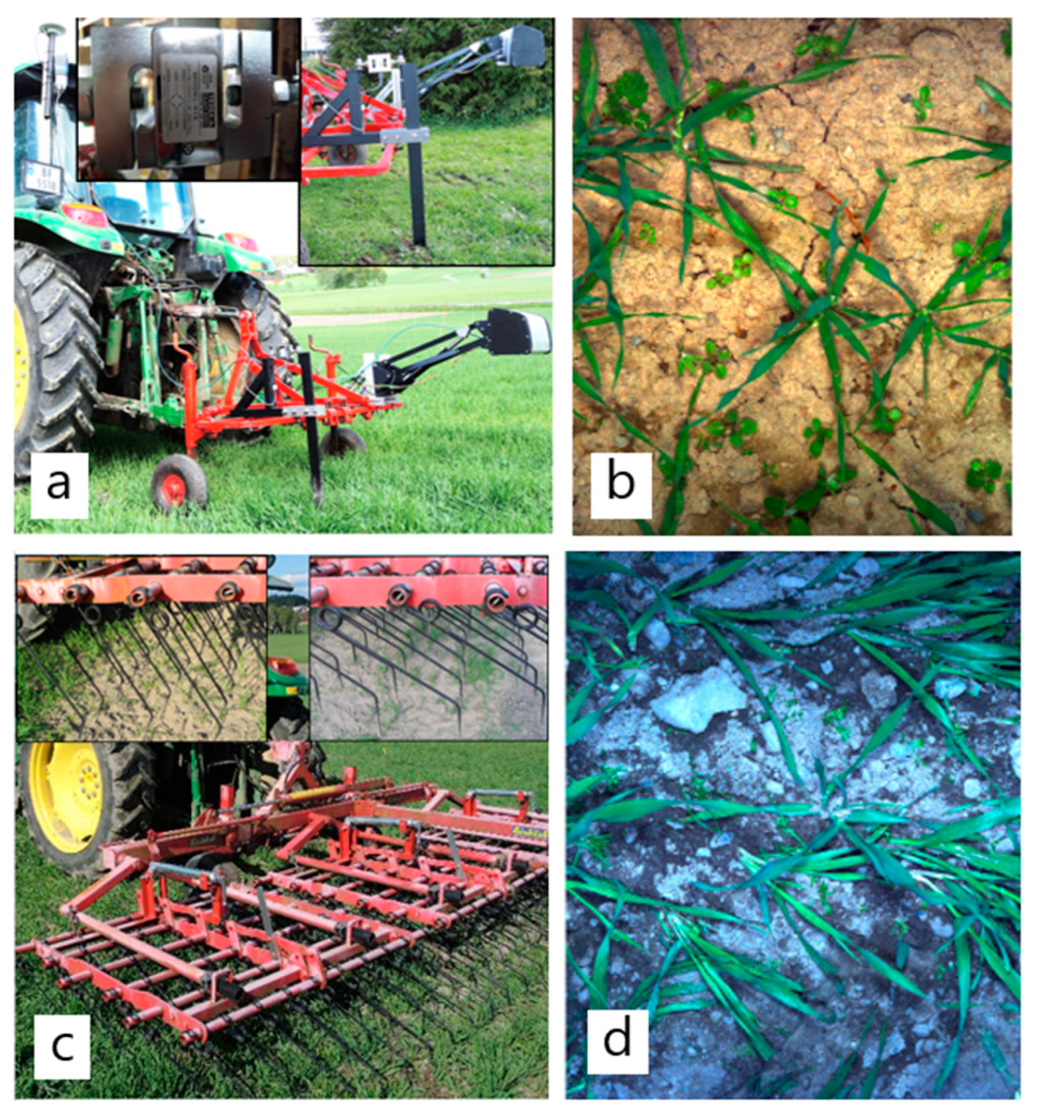
2.2. Image Acquisition and Measurement of Draft Force of Tines

Geo-referenced nadir RGB images and measurements of draft force of tine were acquired a few hours before weed harrowing. A custom-made platform based on an old ‘Troll frame’ (Underhaug Fabrikker AS, Nærbø, Norway) mounted behind a tractor driving forward at 4 km h⁻¹ was used (Figure 1a). The draft force of tines was estimated with an electronic load cell (Tedea-Huntleigh model 616, Vishay Precision Group Inc., Malvern, PA, USA) at about 60 Hz, which was connected to a custom-made rigid tine (dimension 50 mm in the driving direction × 10 mm in the across driving direction, 0.75 m long). The soil depth of the rigid tine was 30–40 mm.

A few hours after the harrowing, RGB images were acquired again, at the same forward speed, along the same swath as the first images that were sampled. Examples of images are shown in Figure 1b,d. The camera setup constituted of a 5 MP megapixel RGB camera (chameleon3, FLIR Systems Inc., Wilsonville, OR, USA) equipped with a 25 mm lens (Computar, CBC Group, Tokyo, Japan) and a custom-built flash to ensure optimum illumination and neutralization of variation in ambient sunlight conditions. The platform was based on a Linux computer that sampled one frame every 0.5 s and location with an RTK-GNSS receiver (PolaRx5, Septentrio, Leuven, Belgium) with an antenna mounted at the top of the tractor cab. The camera’s position ensured that the impact of the wheels or the rigid tine on the plants was not captured in the images. The image resolution was 2448 pixels × 2048 pixels. The distance between the lens and the ground was approximately 0.7 m, covering about 0.27 m × 0.22 m. The number of images per plot was in the range of 12–17 images. In one trial (160602), the image data were unfortunately not recorded everywhere, resulting in 43 and 45 plots with images before and after harrowing, respectively (

Table 2. Image data. The number of RGB images per plot and trial. Images were acquired before (Pre) and after (Post) post-emergence weed harrowing in the five spring barley trials. Images were analyzed by a machine vision algorithm to estimate the mean weed cover per plot before and after weed harrowing, and the weed control efficacy per plot.

Trial Number	150604	160602	160607	170601	180531
Number of plots with images, Pre	48	43 a	48	48	48
Number of images per trial, Pre	650	605	757	692	713
Mean (min., max.) number of images per plot, Pre	13.5 (12, 15)	14.1 (13, 15)	15.8 (14, 17)	14.4 (13, 15)	14.9 (14, 16)
Number of plots with images, Post	48	45 b	48	48	48
Number of images per trial, Post	598	651	739	734	722
Mean (min., max.) number of images per plot, Post	12.5 (9, 15)	14.5 (13, 16)	15.4 (15, 16)	15.3 (14, 17)	15.0 (14, 17)

^a Missing for plots nos. 103, 104, 204, 304, 404; ^b Missing for plots nos. 404, 602, 603.

).

2.3. Weed Harrowing

Weed harrowing, one pass along the crop rows at a speed of 8 km h⁻¹, was conducted after the first series of sensor data (RGB images and load cell data) were collected. The harrow was a 4.5 m wide weed Einböck harrow (Einböck, Dorf an der Pram, Austria) with bent tines (thickness: 7 mm; length: 450 mm) and 25-mm tine spacing. In one trial (170601), there were problems with unfolding the harrow sections (each 1.5 m wide), which made it necessary to conduct two adjacent swaths of harrowing. The only factor imposed on the plots was the harrowing intensity (HI) in terms of the tine angle of the harrow. Before field work, six intensity levels in the range between no harrowing to very high intensity (cf. Figure 1c) were planned in all trials. In practice, however, the number of levels was adjusted to the field situation (soil hardness) and the two most aggressive angles were not used in two of the trials. The levels used were randomly distributed between the six plots in each of the eight blocks. The number of levels per trial varied from 3 to 5 (Table 1). The five harrowing intensity levels were the untreated control (0.0°), 27.5°, 36.5°, 50.0°, and 59.0° (the most aggressive). These angles corresponded with the pre-fixed angles from the factory.

2.4. Post-Processing of GNSS Data and Load Cell Measurements

The accurate coordinates of the sensor measurements were recalculated from the measured distances and angles between the rigid tine and the RGB camera at one side versus the GNSS antenna (mounted on the tractor cab roof). We used only sensor data positioned inside the experimental plots. Data concerning the draft force on tines consisted of raw load cell measurements (unit mV V⁻¹) that were converted to kg through a linear calibration procedure. Then, the individual measurements were calculated into Newton (N) before the calculation of the mean draft force on tines (MF) per plot (N). The mean number of load cell measurements per plot varied between 410 and 514 per trial. In one trial (160602), the data were unfortunately not recorded everywhere, resulting in 40 plots with load cell data (

Table 3. Soil hardness data. The number of measurements of the draft forces on tines per plot and trial.

Trial Number	150604	160602	160607	170601	180531
Number of plots with data	48	40 a	48	48	48
Number of measurements per trial	21,704	16,401	24,684	24,663	24,691
Mean number of measurements per plot	452	410	514	514	514
Minimum number of measurements per plot	266	217	385	463	466
Maximum number of measurements per plot	545	516	552	549	561

^a Missing data in plots nos. 101, 201, 301, 401, 501, 601, 701, 801

).

2.5. Mean Weed Cover per Plot Based on Machine Vision

All images acquired before and after weed harrowing were processed by a machine vision algorithm (the ‘artificial intelligence (AI) algorithm’) based on deep learning techniques. The AI algorithm had been developed for rapid and automatic quantification of the total weed cover and crop cover per image [23]. Algorithm predictions were compared with ground truth data (i.e., images manually annotated (at pixel-level)) using linear regression and the predicted R² statistic (R²_pred). Very good R²_pred values were achieved for pre-harrow images: 95.9% (weed cover) and 98.6% (crop cover). For post-harrow images, the results were similar for crop cover (97.7%) but considerably lower for weed cover (88.4%). The raw outputs from the algorithm were calibrated by using the parameter estimates of a linear regression model predicting the ground truth weed cover from the raw values [23]. Because the algorithm was not trained to discriminate between weed species, the total weed cover per image was estimated. Thereafter, the individual calibrated weed cover values per image were used to calculate the mean weed cover per plot before and after weed harrowing. The number of images per plot and trial is given in Table 2.

2.6. Grain Yield

When the crop was matured, plots were harvested with a research combine harvester with a 1.5 m width cutter. The harvested stripe of each plot (1.5 m × plot length) was generally located on the same side as the sensor measurements. If the equipment that measured the draft force on tines had caused significant crop damage, the other half of the plot was used. This could be observed if the stripe, where the rigid tine passed, significantly differed from the rest of the plot. Fresh weights and the water content of the plot yields were measured, and grain weights were adjusted to 15% water content. One of the samples was unfortunately lost, resulting in 239 grain samples in total.

2.7. Models and Statistical Analysis

The statistical analyses and nonlinear regressions were conducted with the statistical software Minitab^® 19.2 (Minitab Ltd., Coventry, UK) and the procedure NLIN in SAS 9.4 (SAS Institute Inc., Cary, NC, USA).

In the decision model for precision post-emergence weed harrowing, the optimum harrowing intensity in terms of the tine angle of the harrow was predicted by using the mean weed cover before harrowing and mean draft force on tines within the experimental plots. The suggested decision model was achieved through the following steps:

Step 1: The estimation of the biological weed damage threshold per plot (t₀) was conducted by nonlinear regression of grain yield against the mean total weed cover after harrowing. t₀ was defined as the percentage weed cover at which grain yield is reduced.

Step 2: The weed control efficacy (WC) was estimated using a nonlinear regression model based on the applied weed harrow tine angle and the measured mean draft force on tines as independent variables. The measured weed control efficacy was calculated as the difference between pre-harrow mean total weed cover (W_pre) and post-harrow mean total weed cover (W_post) divided by the pre-harrow mean total weed cover. Based on the actual pre-harrow weed cover, the target weed control efficacy (WC₀) to reach the biological weed damage threshold value was calculated. For example, if W_pre = 6%, the target weed control efficacy (WC₀) will be about 60%, 50%, and 40% for biological weed damage threshold values of 2.5%, 3%, and 3.5%, respectively (Figure 2).

Step 3: The parameter values estimated in steps (1) and (2) were then used in the decision model for weed harrowing intensity (also a nonlinear regression model). This model predicts the optimal harrowing intensity (in terms of tine angle) as a function of the actual pre-harrow weed cover, mean draft force of tines, and the parameter value of the biological weed damage threshold.

2.7.1. Step 1: Estimation of the Weed Damage Threshold Parameter (t₀)

A nonlinear model based on the field trial data was used to estimate the biological weed damage threshold parameter (t₀). The measured grain yield (yield) per plot was the response variable, the mean weed cover after weed harrowing per plot (W_post) was the independent variable, and the expectation function was:

$$E(yield)=\left\{\begin{array}{c}\alpha +\beta \times t_0,\mathrm{i}\mathrm{f}{W}_{post}\le t_0\\ \alpha +\beta \times W_{post},\mathrm{i}\mathrm{f}{W}_{post}>t_0\end{array}\right.$$

(1)

In model 1, the expected crop yield is assumed constant for weed cover less or equal to t₀ and decreasing for weed cover greater than t₀. The observed values of W_post (mean weed cover per plot after weed harrowing including the non-harrowed control plots) and crop yield in terms of spring barley grains (kg ha⁻¹) were used to estimate the parameters α, β, and t₀.

2.7.2. Step 2: Weed Control Efficacy

The weed control efficacy, WC, was defined as:

$$WC=\left\{\begin{array}{c}\frac{W_{pre}-W_{post}}{W_{pre}}\times 100=\left(1-\frac{W_{post}}{W_{pre}}\right)\times 100,\mathrm{i}\mathrm{f}{W}_{pre}>W_{post}\\ 0,\mathrm{i}\mathrm{f}{W}_{pre}\le W_{post}\end{array}\right.$$

(2)

where W_pre and W_post are the mean weed cover per plot immediately before and after weed harrowing (one pass), respectively. Given the W_pre and W_post = t₀ (or W_post ≤ t₀₎, the target weed control efficacy, WC₀, is calculated by setting W_post = t₀ in Equation (2):

$$W{C}_0=\left\{\begin{array}{c}\frac{W_{pre}-t_0}{W_{pre}}\times 100=\left(1-\frac{t_0}{W_{pre}}\right)\times 100,\mathrm{i}\mathrm{f}{W}_{pre}>t_0\\ 0,\mathrm{i}\mathrm{f}{W}_{pre}\le t_0\end{array}\right.$$

(3)

For t₀ fixed, Equation (3) gives WC₀ as a function of W_pre, as illustrated in Figure 2.

The expected value of weed control efficacy (µ_WC) was modeled as a nonlinear function of the tine angle (i.e., harrowing intensity (HI)) and mean draft force of tines (MD). For a given value of MD, the function should approach asymptotically 100% when HI increases. For a given value of HI, the function should decrease with increasing MD. Furthermore, it was reasonable to have the function value 0% when HI = 0 (i.e., no weed harrowing) for all values of MD. Many functions meet these requirements. A relatively simple model was used with the following expectation function:

$${\mu }_{WC}=E\left(WC\right)=100\times \tanh \left(\frac{{\alpha }_0+{\alpha }_1\times MD}{100}\times HI\right)$$

(4)

where α₀ and α₁ are parameters estimated from the field trial data. HI is the angle of the harrow tines in degrees, and MD is given in Newton. The asymptote value 100 was used in the denominator to achieve α₀ + α₁∙MD, being the function’s slope when HI = 0. Residual plots did not indicate any significant deviations from the assumptions of normality and homogeneous variance.

2.7.3. Step 3: The Weed Harrowing Intensity Model

Finally, the optimum HI was predicted by setting µ_WC equal to the desired value of the target weed control efficacy, WC₀, because the aim was to find the smallest value HI so that µ_WC ≥ WC₀. By setting µ_WC = WC₀ in Equation (4) and solving the resulting equation for HI, the resulting equation is:

$$HI=\frac{100}{{\alpha }_0+{\alpha }_1\times MD}\times \mathrm{arctanh}\left(\frac{W{C}_0}{100}\right)$$

(5)

In practice, the maximum value of HI is 90°, and in situations where W_pre ≤ t₀, HI should be zero (weed harrowing not necessary). Therefore, Equation (5) was modified to the following model:

$$HI=\left\{\begin{array}{c} 0 , \mathrm{i}\mathrm{f}{W}_{pre}\le t_0\\ \min \left(\frac{100}{{\alpha }_0+{\alpha }_1\times MD}\times \mathrm{arctanh}\left(1-\frac{t_0}{W_{pre}}\right), 90\right), \mathrm{i}\mathrm{f}{W}_{pre}>t_0\end{array}\right.$$

(6)

By replacing the parameters α₀ and α₁ in Equation (6) with their estimates, an estimate of the theoretical optimum harrowing intensity HI needed to achieve the expected weed control efficacy (µ_WC) equal to the target weed control efficacy (WC₀) for a given value of the biological weed damage threshold (t₀) and the observed values of weed cover (W_pre) and mean draft force on tines (MD) was obtained.

3. Results

3.1. The Biological Weed Damage Threshold (t₀)

The observed data of spring barley grain yield per plot and mean weed cover per plot (post-harrow values including the untreated control plots) are shown in Figure 3 along with the estimated expectation function (Equation (1)). The estimated parameters and corresponding standard errors (SE) were: $\widehat{\alpha }=4437.6 \left(SE:171.5\right),\widehat{\beta }=-59.8 \left(SE:16.3\right), \mathrm{and} {\widehat{t}}_0=2.09 \left(SE:2.83\right).$ The latter parameter corresponded to the biological weed damage threshold.

3.2. Expected Weed Control Efficacy

The parameter estimates and summary statistics of the nonlinear regression model predicting the weed control efficacy from weed harrowing intensity and draft force on tines (cf. Equation (4)) are given in

Table 4. Parameters of the model for expected weed control efficacy. Estimated parameters of the nonlinear regression model predicting the weed control efficacy (WC) as a function of weed harrowing intensity (HI) and mean draft force (MD) per plot (cf. Equation (4) and Figure 4). SE = standard error, MSE = mean squared error = 357.1, DFE = degree of freedom = 223.

Parameter	Estimate	SE
α0	1.34	0.07
α1	−0.0003	0.0002

. The predicted weed control efficacies based on the nonlinear regression model (cf. Equation (4) and Table 4) are illustrated in Figure 4. In general, the predicted weed control efficacy increased with increasing weed harrowing intensity. For a fixed weed harrowing intensity, the harder the soil (which is related to the draft force on tines), the less weed control will be achieved (Figure 4).

3.3. The Weed Harrowing Intensity Model (i.e., the Decision Model for Precision Weed Harrowing)

The final nonlinear regression model for weed harrowing intensity (Equation (6)) (i.e., the decision model for precision post-emergence weed harrowing in cereals) is illustrated in Figure 5 for two different mean draft forces on tines. At a given weed cover and biological weed damage threshold, the harrowing intensity must be more aggressive (the tines must be more vertical), so the higher the mean draft force on tines.

4. Discussion

The proposed decision model for precision post-emergence weed harrowing in cereals was a nonlinear regression model. It predicted the optimum tine angle of the weed harrow as a function of three variables: (1) the measured (pre-harrow) weed cover (W_pre), (2) the measured draft force on tines, and (3) the target weed control efficacy necessary to reduce W_pre to the level of the biological weed damage threshold (t₀). This threshold was the estimated mean weed cover per plot at which the grain yield decreased (cf. Figure 3). The current parameter estimates of the model are valid for spring barley. The approach used to establish the model can be used to estimate model parameters for other cereal species and presumable peas. Applying the proposed model on areas with the same mean weed cover but with loose versus dense soil will require relatively gentle versus relatively aggressive tine angles, respectively (cf. Figure 5). This output agreed with a previous fuzzy logic decision model suggested for precision weed harrowing in winter wheat [19].

A nonlinear model was chosen due to its mathematical simplicity. Other nonlinear functions could also have been possible. Rueda-Ayla et al. [24] suggested a decision model for precision weed harrowing in maize, in which the harrow tine angle changed linearly with a sensor signal correlated with the weed density. They did not include a weed damage threshold in their model, neither did others [11,15,19,20]. This aspect and the modeling approach we presented are new for decision models for precision weed harrowing. The benefit of including a weed damage threshold is that sub-field areas with zero or very low weediness are not cultivated, thus reducing disturbance, energy use, and risk of crop damage. Furthermore, at weediness levels above the threshold, the harrowing intensity is always adjusted to the least necessary to reduce weediness down to the threshold. A drawback of including a damage threshold is that it must be known for the crop species and system in question. In future operational use, the weed damage threshold value should be set by the end-user and adjusted to the actual cereal species and expected yield. If known, the economic damage threshold in terms of the mean weed cover per plot could also replace the defined weed damage threshold.

For practical adoption, a map-based approach in which weediness and soil hardness are measured to create a prescription file for variable rate weed harrowing could be foreseen. However, we expect that end-users will not prefer this approach due to two field operations (i.e., more work and higher costs). For a real-time system, several cameras are needed along the width of the weed harrow, probably one per section of the harrow. Motors to change tine angles must also be in place on each section. Whether cameras should be mounted on a boom in front of the tractor or at the harrow itself will depend on the frame processing speed and the time needed to change the angle.

The machine vision algorithm applied was not able to identify the weed species. Consequently, all species were included in one weediness indicator, the total weed cover. This can be seen as a simplification since different weed species can have different potential for crop yield loss. For example, Keller et al. [25] reported that Galium aparine L. reduced the grain yield by 17.5 kg ha⁻¹ plant⁻¹ m², while other dicotyledonous weeds only reduced the yield by 1.2 kg ha⁻¹ plant⁻¹ m². Rueda-Ayala et al. [19,24] also used the overall weediness in their decision models for precision weed harrowing in winter wheat and maize. To the authors’ knowledge, there are no published studies on precision weed harrowing that have adjusted the harrowing intensity to the weed species. However, Spaeth et al. [15] found that their sensor-based criterion for adjustment of the weed tine angle—the immediate crop soil cover following weed harrowing (CSC)—needed to be increased for weed species difficult to control (e.g., G. aparine and Cirsium arvense (L.) Scop). In future work, artificial intelligence could be further exploited to identify specific weed species and develop a weed damage threshold model based on the yield loss potential of specific weeds or combinations of weed species [26]. For an on-the-go (real-time) solution, species-specific damage thresholds will only be sound if the necessary harrowing speed can be maintained (at least about 8 km h⁻¹). If the processing speed of weed species identification algorithms is too slow, a map-based solution where imaging and harrowing are separate field operations could be preferable.

In contrast to others [11,15,19,21], the suggested decision model did not consider the crop cover. In competitive crops like cereals, the weediness indicator, called the relative weed cover (RWC), which includes both the weed cover and the crop cover (weed cover divided by the crop cover + weed cover), is a sound predictor of crop yield loss [27]. RWC thresholds have been implemented in camera-based precision herbicide applications previously in cereals [28] and is now commercially available as an add-on system to ISOBUS field sprayers [6]. We did explore the weed control efficacy based on the mean RWC per plot before and after weed harrowing in the current work. However, this model had much poorer prediction ability than the one used. Probably, the two-variable indicator RWC was less accurate because the machine vision algorithm was not perfect. With a more accurate machine vision algorithm, the weed control efficacy model based on RWC would probably be sound. Then, the weed damage threshold should also be defined in terms of RWC.

Organic spring cereals in Norway and Sweden are usually subject to both pre-emergence and post-emergence weed harrowing [29]. However, the disturbance during the first blind harrowing may be like a double-edged sword: while controlling weeds, it also stimulates a new cohort of weed seeds to germinate. The high proportion of soils often forming a crusted surface in spring is probably the reason for the positive effect of the pre-emergence weed harrowing, although the practice with two weed harrowing operations has been questioned [10,30]. Repeated weed harrowing may affect beneficial arthropods negatively [31]. In fields with a crusted soil surface, pre-emergence weed harrowing will still be necessary. Still, perhaps precision post-emergence weed harrowing could eliminate the need for blind harrowing in areas without hard-packed soils. This would probably be beneficial to the farmer’s economy and the ecosystem. Coleman et al. [32] compared the energy consumption of weeding tools. Among the whole-field methods, traditional weed harrowing consumed the least energy (4.2–5.5 MJ ha⁻¹). With site-specific weed harrowing, a further decrease in energy consumption is expected. Rueda-Ayala et al. [19] reported that fuel consumption was reduced from 3.5 to 1.75 L ha⁻¹ with sensor-based weed harrowing.

Future field trials should validate the suggested decision model. Furthermore, the model could benefit from restricting the maximum harrowing intensity to maintain a maximum value of CSC (i.e., the percentage of the crop canopy covered by soil immediately after the weed harrowing), as implemented by others [12,15,21]. The CSC criterion would be most relevant in areas with severe weed pressure. Inclusion of the CSC criterion would balance the risk of crop damage due to too aggressive harrowing and the risk of crop loss due to weed competition. Future work on the decision model could also include species-specific weed damage thresholds. This would require machine vision algorithms capable of discriminating specific weed species or groups. If the processing speeds of such algorithms are not compatible with weed harrowing speeds (at least about 8 km h⁻¹), a map-based approach for precision weed harrowing could be a solution.

5. Conclusions

A decision model for precision post-emergence weed harrowing in cereals based on experimental data in spring barley and regression analysis was developed. The model predicted the optimal harrowing intensity in terms of the tine angle of the weed harrow for a given weed cover (estimated by RGB imagery and artificial intelligence), a given draft force on the tines (estimated by electronic load cell), and a pre-set value for the assumed acceptable weed cover (i.e., the biological weed damage threshold). Future field trials should validate the suggested decision model. The model did not consider that different weed species may affect the crop yield differently. In future work, artificial intelligence could be exploited further to develop algorithms capable of discriminating weed species. If a real-time approach is intended, the processing speed must comply with normal weed harrowing speeds (about 8 km h⁻¹).