
Use of Indices in RGB and Random Forest Regression to Measure the Leaf Area Index in Maize


Abstract
1. Introduction
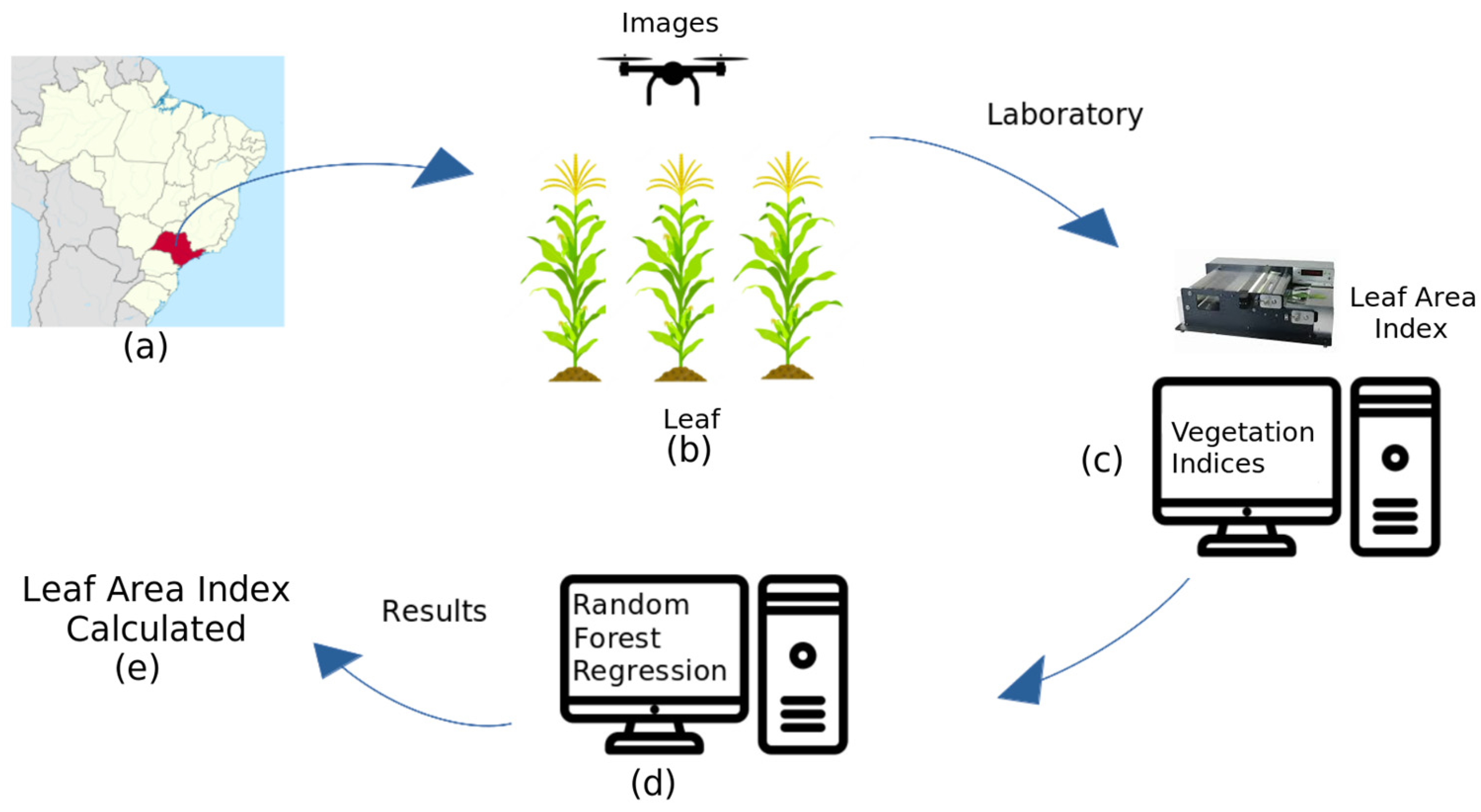
2. Materials and Methods
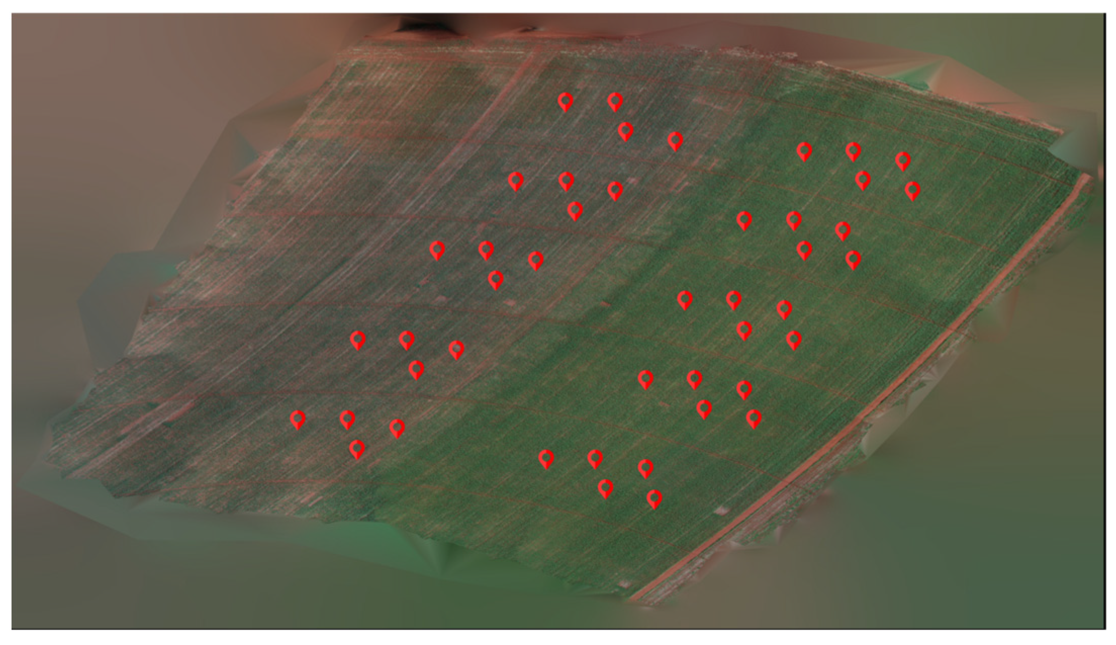
2.1. Field Experiments
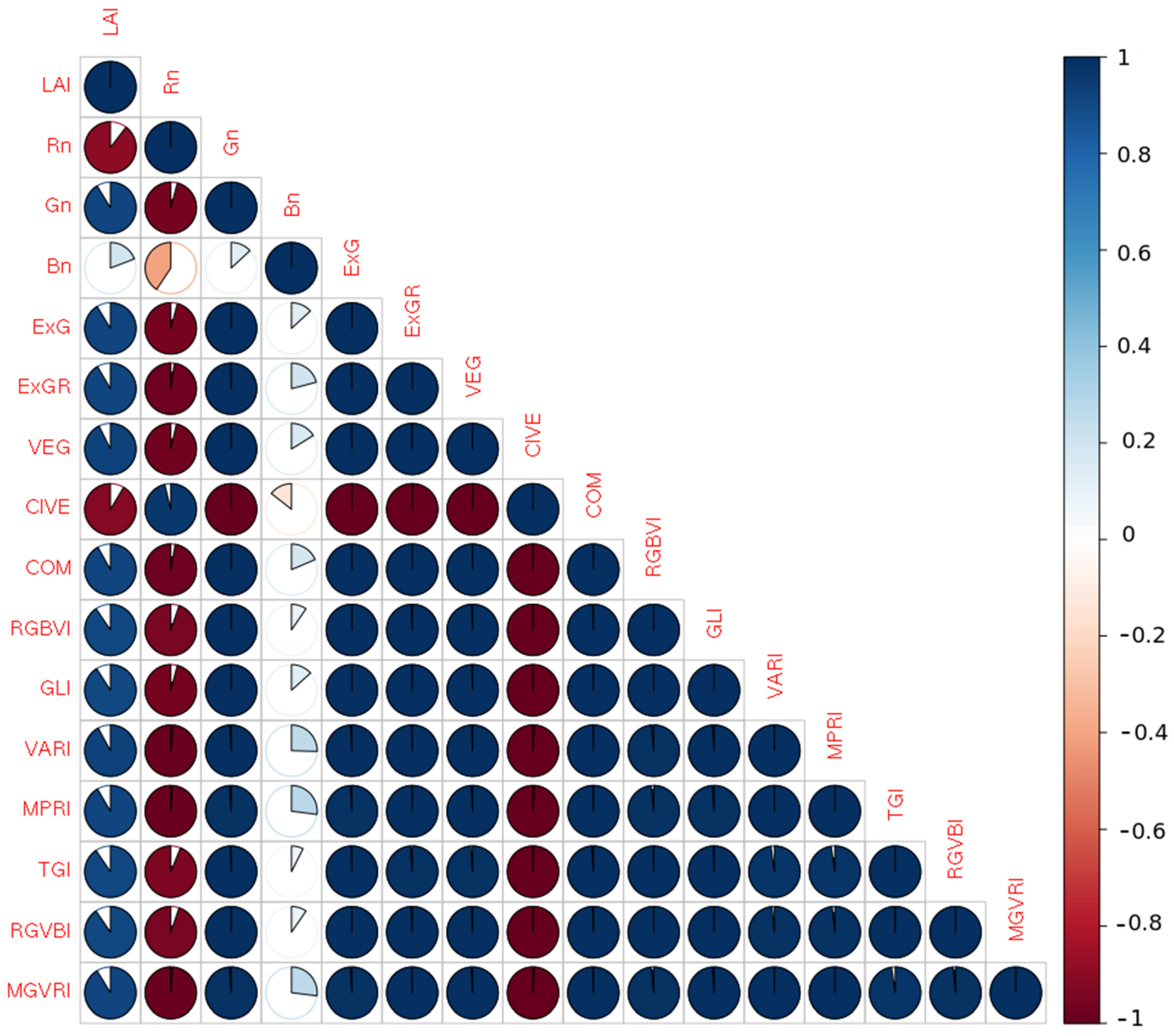
2.2. Statistical Analysis
3. Results
4. Discussion
5. Conclusions
Author Contributions
Funding
Data Availability Statement
Conflicts of Interest
References
- Gitelson, A.A.; Viña, A.; Arkebauer, T.J.; Rundquist, D.C.; Keydan, G.; Leavitt, B. Remote Estimation of Leaf Area Index and Green Leaf Biomass in Maize Canopies. Geophys. Res. Lett. 2003, 30, 1248. [Google Scholar] [CrossRef]
- Bian, M.; Chen, Z.; Fan, Y.; Ma, Y.; Liu, Y.; Chen, R.; Feng, H. Integrating Spectral, Textural, and Morphological Data for Potato LAI Estimation from UAV Images. Agronomy 2023, 13, 3070. [Google Scholar] [CrossRef]
- Rasti, S.; Bleakley, C.J.; Holden, N.M.; Whetton, R.; Langton, D.; O’Hare, G. A Survey of High Resolution Image Processing Techniques for Cereal Crop Growth Monitoring. Inf. Process. Agric. 2021, 9, 300–315. [Google Scholar] [CrossRef]
- Wang, Y.; Zhou, H.; Ma, X.; Liu, H. Combining Data Assimilation with Machine Learning to Predict the Regional Daily Leaf Area Index of Summer Maize (Zea mays L.). Agronomy 2023, 13, 2688. [Google Scholar] [CrossRef]
- Han, K.; Liu, B.; Liu, P.; Wang, Z. The Optimal Plant Density of Maize for Dairy Cow Forage Production. Agron. J. 2020, 112, 1849–1861. [Google Scholar] [CrossRef]
- Jia, Q.; Sun, L.; Mou, H.; Ali, S.; Liu, D.; Zhang, Y.; Zhang, P.; Ren, X.; Jia, Z. Effects of Planting Patterns and Sowing Densities on Grain-Filling, Radiation Use Efficiency and Yield of Maize (Zea mays L.) in Semi-Arid Regions. Agric. Water Manag. 2017, 201, 287–298. [Google Scholar] [CrossRef]
- Panigrahi, N.; Das, B.S. Evaluation of Regression Algorithms for Estimating Leaf Area Index and Canopy Water Content from Water Stressed Rice Canopy Reflectance. Inf. Process. Agric. 2021, 8, 284–298. [Google Scholar] [CrossRef]
- Fang, H.; Baret, F.; Plummer, S.; Schaepman-Strub, G. An Overview of Global Leaf Area Index (LAI): Methods, Products, Validation, and Applications. Rev. Geophys. 2019, 57, 739–799. [Google Scholar] [CrossRef]
- Bréda, N. Ground-based Measurements of Leaf Area Index: A Review of Methods, Instruments and Current Controversies. J. Exp. Bot. 2003, 54, 2403–2417. [Google Scholar] [CrossRef]
- Jonckheere, I.; Fleck, S.; Nackaerts, K.; Muys, B.; Coppin, P.; Weiss, M.; Baret, F. Review of Methods for in Situ Leaf Area Index Determination Part I. Theories, Sensors and Hemispherical Photography. Agric. For. Meteorol. 2004, 121, 19–35. [Google Scholar] [CrossRef]
- Weiss, M.; Baret, F.; Smith, G.; Jonckheere, I.; Coppin, P. Review of Methods for in Situ Leaf Area Index (LAI) Determination: Part II. Estimation of LAI, Errors and Sampling. Agric. For. Meteorol. 2004, 121, 37–53. [Google Scholar] [CrossRef]
- Zheng, G.; Moskal, L.M. Retrieving Leaf Area Index (LAI) Using Remote Sensing: Theories, Methods and Sensors. Sensors 2009, 9, 2719. [Google Scholar] [CrossRef] [PubMed]
- Verma, B.R.; Thakore, T.; Prasad, R.; Srivastava, P.K.; Yadav, S.A.; Singh, P.; Singh, R. Investigation of Optimal Vegetation Indices for Retrieval of Leaf Chlorophyll and Leaf Area Index Using Enhanced Learning Algorithms. Comput. Electron. Agric. 2022, 192, 106581. [Google Scholar] [CrossRef]
- Xue, J.; Su, B. Significant Remote Sensing Vegetation Indices: A Review of Developments and Applications. J. Sens. 2017, 2017, 1353691. [Google Scholar] [CrossRef]
- Abebe, G.; Tadesse, T.; Gessesse, B. Estimating Leaf Area Index and Biomass of Sugarcane Based on Gaussian Process Regression Using Landsat 8 and Sentinel 1A Observations. Int. J. Image Data Fusion 2022, 14, 58–88. [Google Scholar] [CrossRef]
- Mulla, D.J. Twenty Five Years of Remote Sensing in Precision Agriculture: Key Advances and Remaining Knowledge Gaps. Biosyst. Eng. 2013, 114, 358–371. [Google Scholar] [CrossRef]
- Yadav, S.A.; Prasad, R.; Yadav, V.P.; Verma, B.; Singh, S.; Sharma, J.; Srivastava, B.K. Far-field Bistatic Scattering Simulation for Rice Crop Biophysical Parameters Retrieval Using Modified Radiative Transfer Model at X- and C-band. Remote Sens. Environ. 2022, 272, 112959. [Google Scholar] [CrossRef]
- Yue, J.; Yang, G.; Tian, Q.; Feng, H.; Xu, K.; Zhou, C. Estimate of Winter-Wheat Above-Ground Biomass Based on UAV Ultrahigh-Ground-Resolution Image Textures and Vegetation Indices. ISPRS J. Photogramm. Remote Sens. 2019, 150, 226–244. [Google Scholar] [CrossRef]
- Hunt, E.R.; Cavigelli, M.A.; Daughtry, C.S.; McMurtrey, J.E.; Walthall, C.L. Evaluation of Digital Photography from Model Aircraft for Remote Sensing of Crop Biomass and Nitrogen Status. Precis. Agric. 2005, 6, 359–378. [Google Scholar] [CrossRef]
- Jin, X.; Zarco-Tejada, P.J.; Schmidhalter, U.; Reynolds, M.P.; Hawkesford, M.J.; Varshney, R.K.; Yang, T.; Nie, C.; Li, Z.; Ming, B.; et al. High-Throughput Estimation of Crop Traits: A Review of Ground and Aerial Phenotyping Platforms. IEEE Geosci. Remote Sens. Mag. 2021, 9, 200–231. [Google Scholar] [CrossRef]
- Prey, L.; von Bloh, M.; Schmidhalter, U. Evaluating RGB Imaging and Multispectral Active and Hyperspectral Passive Sensing for Assessing Early Plant Vigor in Winter Wheat. Sensors 2018, 18, 2931. [Google Scholar] [CrossRef]
- Li, X.; Xu, X.; Xiang, S.; He, S.; Wang, W.; Xu, M.; Liu, C.; Yu, L.; Liu, W.; Yang, W. Soybean Leaf Estimation Based on RGB Images and Machine Learning Methods. Plant Methods 2023, 19, 59. [Google Scholar] [CrossRef]
- Rasmussen, J.J.; Ntakos, G.; Nielsen, J.F.; Svensgaard, J.; Poulsen, R.; Christensen, S. Are Vegetation Indices Derived from Consumer-Grade Cameras Mounted on UAVs Sufficiently Reliable for Assessing Experimental Plots? Eur. J. Agron. 2016, 74, 75–92. [Google Scholar] [CrossRef]
- Du, L.; Yang, H.; Song, X.; Wei, N.; Yu, C.; Wang, W.; Zhao, Y. Estimating Leaf Area Index of Maize Using UAV-Based Digital Imagery and Machine Learning Methods. Sci. Rep. 2022, 12, 15937. [Google Scholar] [CrossRef]
- Siegmann, B.; Jarmer, T. Comparison of Different Regression Models and Validation Techniques for the Assessment of Wheat Leaf Area Index from Hyperspectral Data. Int. J. Remote Sens. 2015, 36, 4519–4534. [Google Scholar] [CrossRef]
- Breiman, L. Random forests. Mach. Learn. 2001, 45, 5–32. [Google Scholar] [CrossRef]
- Chemura, A.; Chemura, A.; Mutanga, O.; Dube, T. Separability of Coffee Leaf Rust Infection Levels with Machine Learning Methods at Sentinel-2 MSI Spectral Resolutions. Precis. Agric. 2017, 18, 859–881. [Google Scholar] [CrossRef]
- Akbarian, S.; Rahimi Jamnani, M.; Xu, C.-Y.; Wang, W.; Lim, S. Plot Level Sugarcane Yield Estimation by Machine Learning on Multispectral Images: A Case Study of Bundaberg, Australia. Inf. Process. Agric. 2023, in press. [Google Scholar] [CrossRef]
- Borup, D.; Christensen, B.J.; Mühlbach, N.S.; Nielsen, M.S. Targeting predictors in random forest regression. Int. J. Forecast. 2023, 39, 841–868. [Google Scholar] [CrossRef]
- Luo, P.; Liao, J.; Shen, G. Combining Spectral and Texture Features for Estimating Leaf Area Index and Biomass of Maize Using Sentinel-1/2, and Landsat-8 Data. IEEE Access 2020, 8, 53614–53626. [Google Scholar] [CrossRef]
- Chen, Y.; Ma, L.; Yu, D.; Feng, K.; Wang, X.; Song, J. Improving Leaf Area Index Retrieval Using Multi-Sensor Images and Stacking Learning in Subtropical Forests of China. Remote Sens. 2022, 14, 148. [Google Scholar] [CrossRef]
- Frost, T.; Lindon, J.C.; Tranter, G.E.; Koppenaal, D.W. Quantitative Analysis. In Encyclopedia of Spectroscopy and Spectrometry; Academic Press: Oxford, UK, 2017; pp. 811–815. [Google Scholar]
- Roy, K.; Kar, S.; Das, R.N. Selected Statistical Methods in QSAR. In Understanding the Basics of QSAR for Applications in Pharmaceutical Sciences and Risk Assessment; Academic Press: Oxford, UK, 2015; pp. 191–229. [Google Scholar]
- Verrelst, J.; Muñoz, J.; Alonso, L.; Delegido, J.; Rivera, J.P.; Camps-Valls, G.; Moreno, J. Machine Learning Regression Algorithms for Biophysical Parameter Retrieval: Opportunities for Sentinel-2 and -3. Remote Sens. Environ. 2012, 118, 127–139. [Google Scholar] [CrossRef]
- Ji, S.; Gu, C.; Xi, X.; Zhang, Z.; Hong, Q.; Huo, Z.; Zhao, H.; Zhang, R.; Li, B.; Tan, C. Quantitative Monitoring of Leaf Area Index in Rice Based on Hyperspectral Feature Bands and Ridge Regression Algorithm. Remote Sens. 2022, 14, 2777. [Google Scholar] [CrossRef]
- Kataoka, T.; Kaneko, T.; Okamoto, H.; Hata, S. Crop Growth Estimation System Using Machine Vision. In Proceedings of the 2003 IEEE/ASME International Conference on Advanced Intelligent Mechatronics (AIM 2003), Kobe, Japan, 20–24 July 2003. [Google Scholar] [CrossRef]
- Montalvo, M.; Guerrero, J.M.; Romeo, J.; Emmi, L.; Guijarro, M.; Pajares, G. Automatic Expert System for Weeds/Crops Identification in Images from Maize Fields. Expert Syst. Appl. 2013, 40, 75–82. [Google Scholar] [CrossRef]
- Woebbecke, D.M.; Meyer, G.; Von Bargen, K.; Mortensen, D.A. Shape Features for Identifying Young Weeds Using Image Analysis. Trans. ASAE 1995, 38, 271–281. [Google Scholar] [CrossRef]
- Meyer, G.E.; Neto, J.C. Verification of Color Vegetation Indices for Automated Crop Imaging Applications. Comput. Electron. Agric. 2008, 63, 282–293. [Google Scholar] [CrossRef]
- Louhaichi, M.; Borman, M.M.; Johnson, D.E. Spatially Located Platform and Aerial Photography for Documentation of Grazing Impacts on Wheat. Geocarto Int. 2001, 16, 65–70. [Google Scholar] [CrossRef]
- Yang, Z.; Willis, P.; Mueller, R. Impact of Band-Ratio Enhanced Awifs Image to Crop Classification Accuracy. 2008. Available online: http://www.asprs.org/a/publications/proceedings/pecora17/0041.pdf (accessed on 25 January 2024).
- Bendig, J.; Yu, K.; Aasen, H.; Bolten, A.; Bennertz, S.; Broscheit, J.; Gnyp, M.L.; Bareth, G. Combining UAV-Based Plant Height from Crop Surface Models, Visible, and near Infrared Vegetation Indices for Biomass Monitoring in Barley. Int. J. Appl. Earth Obs. Geoinf. 2015, 39, 79–87. [Google Scholar] [CrossRef]
- Hunt, E.R.; Doraiswamy, P.C.; McMurtrey, J.E.; Daughtry, C.S.T.; Perry, E.M.; Akhmedov, B. A Visible Band Index for Remote Sensing Leaf Chlorophyll Content at the Canopy Scale. Int. J. Appl. Earth Obs. Geoinf. 2013, 21, 103–112. [Google Scholar] [CrossRef]
- Gitelson, A.A.; Kaufman, Y.J.; Stark, R.; Rundquist, D. Novel Algorithms for Remote Estimation of Vegetation Fraction. Remote Sens. Environ. 2002, 80, 76–87. [Google Scholar] [CrossRef]
- Hague, T.; Tillett, N.D.; Wheeler, H. Automated Crop and Weed Monitoring in Widely Spaced Cereals. Precis. Agric. 2006, 7, 21–32. [Google Scholar] [CrossRef]
- Huete, A.R. Remote Sensing for Environmental Monitoring. Environ. Monit. Charact. 2004, 183–206. [Google Scholar] [CrossRef]
- Shao, G.; Han, W.; Zhang, H.; Liu, S.; Wang, Y.; Zhang, L.; Cui, X. Mapping Maize Crop Coefficient Kc Using Random Forest Algorithm Based on Leaf Area Index and UAV-Based Multispectral Vegetation Indices. Agric. Water Manag. 2021, 252, 106906. [Google Scholar] [CrossRef]
- Qiao, L.; Gao, D.; Zhao, R.; Tang, W.; An, L.; Li, M.; Sun, H. Improving Estimation of LAI Dynamic by Fusion of Morphological and Vegetation Indices Based on UAV Imagery. Comput. Electron. Agric. 2022, 192, 106603. [Google Scholar] [CrossRef]
- Smith, H.L.; McAusland, L.; Murchie, E.H. Don’t Ignore the Green Light: Exploring Diverse Roles in Plant Processes. J. Exp. Bot. 2017, 68, 2099–2110. [Google Scholar] [CrossRef] [PubMed]
- Zhang, Y.; Xu, Z.; Li, J.; Wang, R. Optimum Planting Density Improves Resource Use Efficiency and Yield Stability of Rainfed Maize in Semiarid Climate. Front. Plant Sci. 2021, 12, 752606. [Google Scholar] [CrossRef] [PubMed]
- Brewer, K.; Clulow, A.; Sibanda, M.; Gokool, S.; Naiken, V.; Mabhaudhi, T. Predicting the Chlorophyll Content of Maize over Phenotyping as a Proxy for Crop Health in Smallholder Farming Systems. Remote Sens. 2022, 14, 518. [Google Scholar] [CrossRef]
- Hasan, U.; Sawut, M.; Chen, S. Estimating the Leaf Area Index of Winter Wheat Based on Unmanned Aerial Vehicle RGB-Image Parameters. Sustainability 2019, 11, 6829. [Google Scholar] [CrossRef]
- Ballesteros, R.; Moreno, M.; Barroso, F.; González-Gómez, L.; Ortega, J. Assessment of Maize Growth and Development with High- and Medium-Resolution Remote Sensing Products. Agronomy 2021, 11, 940. [Google Scholar] [CrossRef]
- Marcial-Pablo, M.D.J.; Gonzalez-Sanchez, A.; Jimenez-Jimenez, S.I.; Ontiveros-Capurata, R.E.; Ojeda-Bustamante, W. Estimation of Vegetation Fraction Using RGB and Multispectral Images from UAV. Int. J. Remote Sens. 2018, 40, 420–438. [Google Scholar] [CrossRef]
- Sanches, G.M.; Duft, D.G.; Kölln, O.T.; Cláudia, A.; Quassi, G.; Okuno, F.M.; Henrique, C.J.F. The Potential for RGB Images Obtained Using Unmanned Aerial Vehicle to Assess and Predict Yield in Sugarcane Fields. Int. J. Remote Sens. 2018, 39, 5402–5414. [Google Scholar] [CrossRef]
- Chen, S.; Chen, Y.; Chen, J.; Zhang, Z.; Fu, Q.; Bian, J.; Cui, T.; Ma, Y. Retrieval of Cotton Plant Water Content by UAV-Based Vegetation Supply Water Index (VSWI). Int. J. Remote Sens. 2020, 41, 4389–4407. [Google Scholar] [CrossRef]
- Gholinejad, S.; Fatemi, S.B. Optimum Indices for Vegetation Cover Change Detection in the Zayandeh-Rud River Basin: A Fusion Approach. Int. J. Image Data Fusion 2019, 10, 199–216. [Google Scholar] [CrossRef]
- Liu, S.; Jin, X.; Nie, C.; Wang, S.; Yu, X.; Cheng, M.; Shao, M.; Wang, Z.; Tuohuti, N.; Bai, Y.; et al. Estimating Leaf Area Index Using Unmanned Aerial Vehicle Data: Shallow vs. Deep Machine Learning Algorithms. Plant Physiol. 2021, 187, 1551–1576. [Google Scholar] [CrossRef]
- Chai, T.; Draxler, R.R. Root Mean Square Error (RMSE) or Mean Absolute Error (MAE)? Geosci. Model Dev. Discuss. 2014, 7, 1525–1534. [Google Scholar] [CrossRef]
- Wolff, F.; Kolari, T.H.M.; Villoslada, M.; Tahvanainen, T.; Korpelainen, P.; Zamboni, P.A.P.; Kumpula, T. RGB Vs. Multispectral Imagery: Mapping Aapa Mire Plant Communities with Uavs. Ecol. Indic. 2023, 148, 110140. [Google Scholar] [CrossRef]
- Furukawa, F.; Laneng, L.A.; Ando, H.; Yoshimura, N.; Kaneko, M.; Morimoto, J. Comparison of RGB and Multispectral Unmanned Aerial Vehicle for Monitoring Vegetation Coverage Changes on a Landslide Area. Drones 2021, 5, 97. [Google Scholar] [CrossRef]


| Index | Equation |
|---|---|
| Bn (Normalized Blue) | B/(R + G + B) |
| Gn (Normalized Green) | G/(R + G + B) |
| Rn (Normalized Red) | R/(R + G + B) |
| CIVE (The index Color Index of Vegetation) | (0.441 × Rn) − (0.881 × Gn) + (0.385 × Bn) + 18.78745 |
| COM (Combination) | (0.25 × ExG) + (0.3 × ExGR) + (0.33 × CIVE) + (0.12 × VEG) |
| ExG (Excess of Green) | (2 × gn) − Rn − Bn |
| ExGR (Excess of Green and Red) | ExG − ((1.4 × Rn) − Gn) |
| GLI (Green Leaf Index) | ((2 × G) − R − B)/((2 × G) + R + B) |
| MGVRI (Modified Green Red Vegetation Index) | ((G × G) − (R × R))/((G × G) + (R × R)) |
| MPRI (or NDRI) (Modified Photochemical Reflectance Index) | G − R/G + R |
| RGBVI (Red–Green–Blue Vegetation Index) | ((G × G) − (R × B))/((G × G) + (R × B)) |
| RGVBI (Red–Green–Blue Vegetation Index) | (G − (B × R))/((G × G) + (B × R)) |
| TGI (Triangular Greenness Index) | G − (0.39 × R) − (0.61 × B) |
| VARI (Visible Atmospherically Resistant Index) | (G − R)/((G + R) − B) |
| VEG (Vegetative Index) | Gn/((Rn 0.667) × (Bn0.333)) |
| Date | Phenological Stage |
|---|---|
| 29 March 2021 | V6 |
| 5 April 2021 | V8 |
| 12 April 2021 | V9 |
| 19 April 2021 | V10 |
| 3 May 2021 | VT |
| Model Index | Predictors |
|---|---|
| 1 | VEG |
| 2 | MGVRI VARI |
| 3 | MGVRI MPRI TGI |
| 4 | ExGR COM TGI VEG |
| 5 | ExGR COM Rn TGI VEG |
| 6 | ExGR COM MGVRI TGI VARI VEG |
| 7 | ExGR COM MGVRI Rn TGI VARI VEG |
| 8 | ExGR COM MGVRI MPRI Rn TGI VARI VEG |
| R2 | MAE (m2 m−2) | RMSE (m2 m−2) | |
|---|---|---|---|
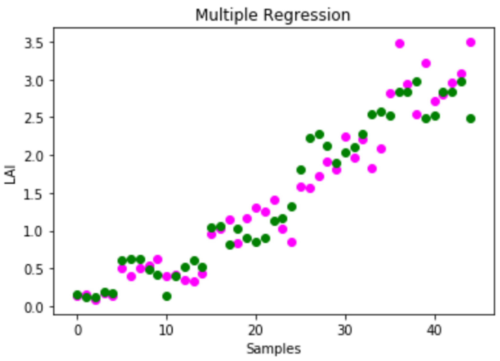
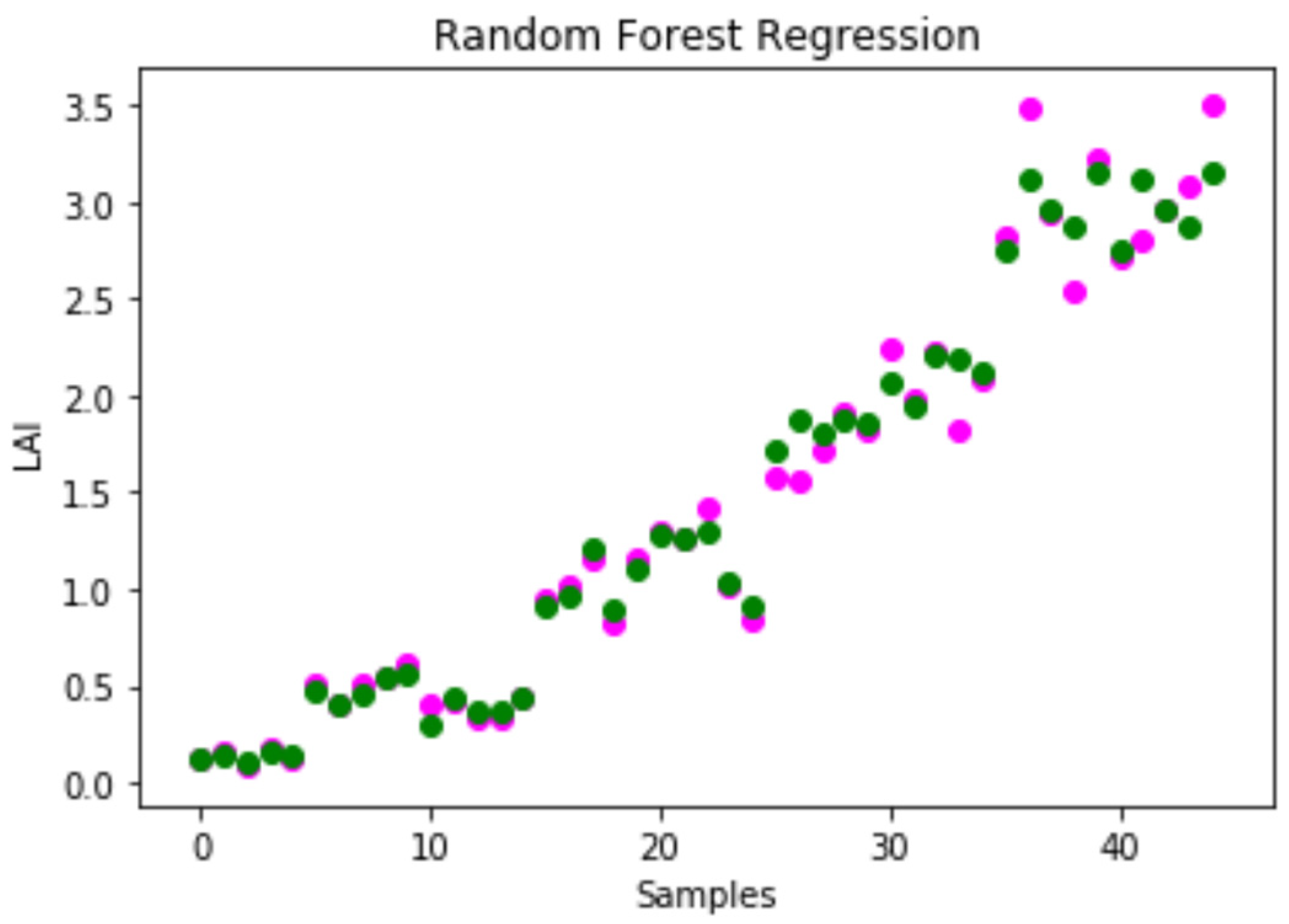
| MLR | 0.89 | 0.25 | 0.34 |
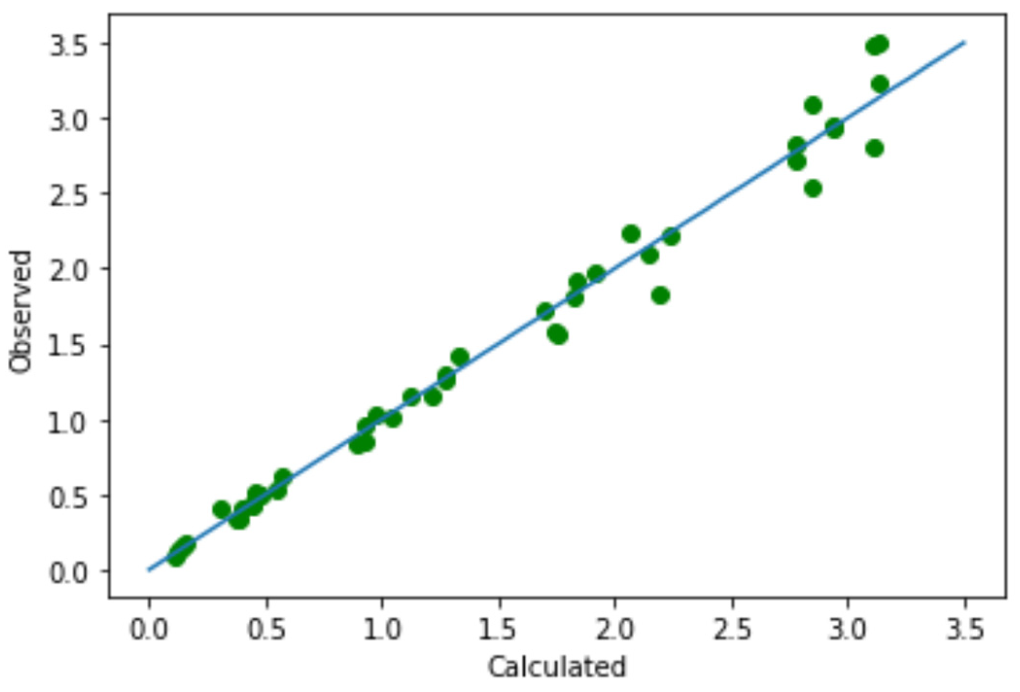
| RFR | 0.98 | 0.08 | 0.14 |
| RR | 0.86 | 0.27 | 0.37 |
| SVM | 0.90 | 0.23 | 0.32 |
| R2 | RMSE (m2 m−2) | |
|---|---|---|
| VEG | 0.86 | 0.39 |
| COM | 0.84 | 0.41 |
| ExGR | 0.84 | 0.41 |
| TGI | 0.82 | 0.44 |
Disclaimer/Publisher’s Note: The statements, opinions and data contained in all publications are solely those of the individual author(s) and contributor(s) and not of MDPI and/or the editor(s). MDPI and/or the editor(s) disclaim responsibility for any injury to people or property resulting from any ideas, methods, instructions or products referred to in the content. |
© 2024 by the authors. Licensee MDPI, Basel, Switzerland. This article is an open access article distributed under the terms and conditions of the Creative Commons Attribution (CC BY) license (https://creativecommons.org/licenses/by/4.0/).
Share and Cite
de Magalhães, L.P.; Rossi, F. Use of Indices in RGB and Random Forest Regression to Measure the Leaf Area Index in Maize. Agronomy 2024, 14, 750. https://doi.org/10.3390/agronomy14040750
de Magalhães LP, Rossi F. Use of Indices in RGB and Random Forest Regression to Measure the Leaf Area Index in Maize. Agronomy. 2024; 14(4):750. https://doi.org/10.3390/agronomy14040750
Chicago/Turabian Stylede Magalhães, Leonardo Pinto, and Fabrício Rossi. 2024. "Use of Indices in RGB and Random Forest Regression to Measure the Leaf Area Index in Maize" Agronomy 14, no. 4: 750. https://doi.org/10.3390/agronomy14040750
APA Stylede Magalhães, L. P., & Rossi, F. (2024). Use of Indices in RGB and Random Forest Regression to Measure the Leaf Area Index in Maize. Agronomy, 14(4), 750. https://doi.org/10.3390/agronomy14040750