Garlic Crops’ Mapping and Change Analysis in the Erhai Lake Basin Based on Google Earth Engine

Abstract

Garlic (Allium sativum) is an important economic crop in China. In terms of using remote sensing technology to identify it, there is still room for improvement, and the high-precision classification of garlic has become an important issue. However, to the best of our knowledge, few studies have focused on garlic area mapping. Here, we propose a method for identifying garlic crops using samples and a multi-feature dataset under limited conditions. The results indicate the following: (1) In the land-use classification of the Erhai Lake Basin, the importance ranking of the characteristic bands, from high to low, is as follows: spectral features, vegetation features, texture features, and terrain features. (2) The random forest method based on feature selection demonstrates high accuracy in land-use classification within the Erhai Lake Basin in Yunnan Province. The overall classification accuracy reached 95.79%, with a Kappa coefficient of 0.95. (3) From 1999 to 2023, the expansion of garlic cultivation in the Erhai Lake Basin showed a trend of initially strengthening from north to south, which was followed by weakening. The vertical development of garlic cultivation reached saturation, showing a slow trend toward horizontal expansion between 2005 and 2018. The planting distributions in various townships in the Erhai Lake Basin gradually shifted from relatively uniform distributions to upstream development. This study utilized the Google Earth Engine (GEE) cloud computing platform and machine learning algorithms to compensate for the lack of statistical data on garlic cultivation in the Erhai Lake Basin. Moreover, it accurately, rapidly, and efficiently extracted planting information, demonstrating significant potential for practical applications.

1. Introduction

Garlic (Allium sativum), as a globally significant economic crop and vegetable, is widely cultivated worldwide. With the growth of the global population and changes in dietary patterns, the cultivation area and production of garlic have been continually increasing. In the cultivation process of this crop, there is a significant demand for fertilizers and pesticides. With the global emphasis on ecological conservation and sustainable development in recent years, there has been a call for remote sensing identification to facilitate industry adjustments and precise management in garlic cultivation. However, the above-ground part of garlic is similar to other vegetation, making it difficult to extract its information directly from optical data and identify it with high precision.

Currently, remote sensing technology has been extensively utilized in the identification of crop growth, the monitoring of the growth status, and other processes related to crop development. Based on a series of remote sensing images, such as MODIS, Landsat, GF, Sentinel, etc. images, it is possible to support agricultural development and crop identification efficiently and intelligently [1,2]. Scholars collaborate using multi-source, high-resolution data, exploiting the abundant temporal information for crop classification [3]. Zhao et al. [4] utilized Landsat imagery combined with multitemporal data to create 30 m spatial resolution bamboo distribution maps for Uganda, Ethiopia, and Kenya. They proposed a composite hybrid evolution algorithm and a temporal similarity threshold to identify winter wheat, achieving an overall accuracy of 99% [5]. Additionally, researchers achieved the high-precision classification of rice by combining the phenological features into a time series curve [6]. Both pixel-based and object-oriented classification methods are commonly employed to enhance classification accuracy. For instance, Chen [7] developed a POK-based method integrating pixel- and object-oriented approaches, yielding favorable results. Wessel [8] successfully classified deciduous trees, oak trees, and others using both pixel-based and object-oriented methods. Mathieu [9] verified the high accuracy of object-oriented classification methods in mapping multiple tree species. However, these methods rely on local computer analysis, which leads to issues such as low efficiency, long processing times, and uncertain identification accuracy. As the volume of data increases, traditional computing models struggle to handle large-scale, high-resolution storage, leading to issues such as lag, data loss, etc. The emergence of remote sensing cloud computing platforms has successfully addressed these problems, enabling the processing and analysis of large-scale, extensive calculations. Currently, the most mature remote sensing cloud computing platform is Google Earth Engine (GEE), widely utilized both domestically and internationally [10]. Apart from classifying and extracting information on major crops such as rice, wheat, and maize, remote sensing can also be used for the identification of other crops like palm trees [11] and tea plantations [12], significantly enhancing the classification effectiveness and accuracy while further refining the remote sensing detection system for crop cultivation. Therefore, the garlic crop remote sensing extraction models supported by the GEE platform are crucial for achieving high-precision planting monitoring.

In this study, we classified garlic crops in the Erhai Lake Basin by utilizing Landsat images and constructing an optimal multidimensional feature set suitable for extraction through Google Earth Engine (GEE). The objectives of this study address the following questions: (1) Is the utilization of the KNDVI effective for garlic crop identification? (2) Are the feature dataset and random forest classification effective for the biodiversity of Yunnan’s cultivated crops? (3) Can we explore the spatiotemporal distribution of garlic crops in the Erhai Lake Basin and achieve satisfactory accuracy?

2. Materials and Methods

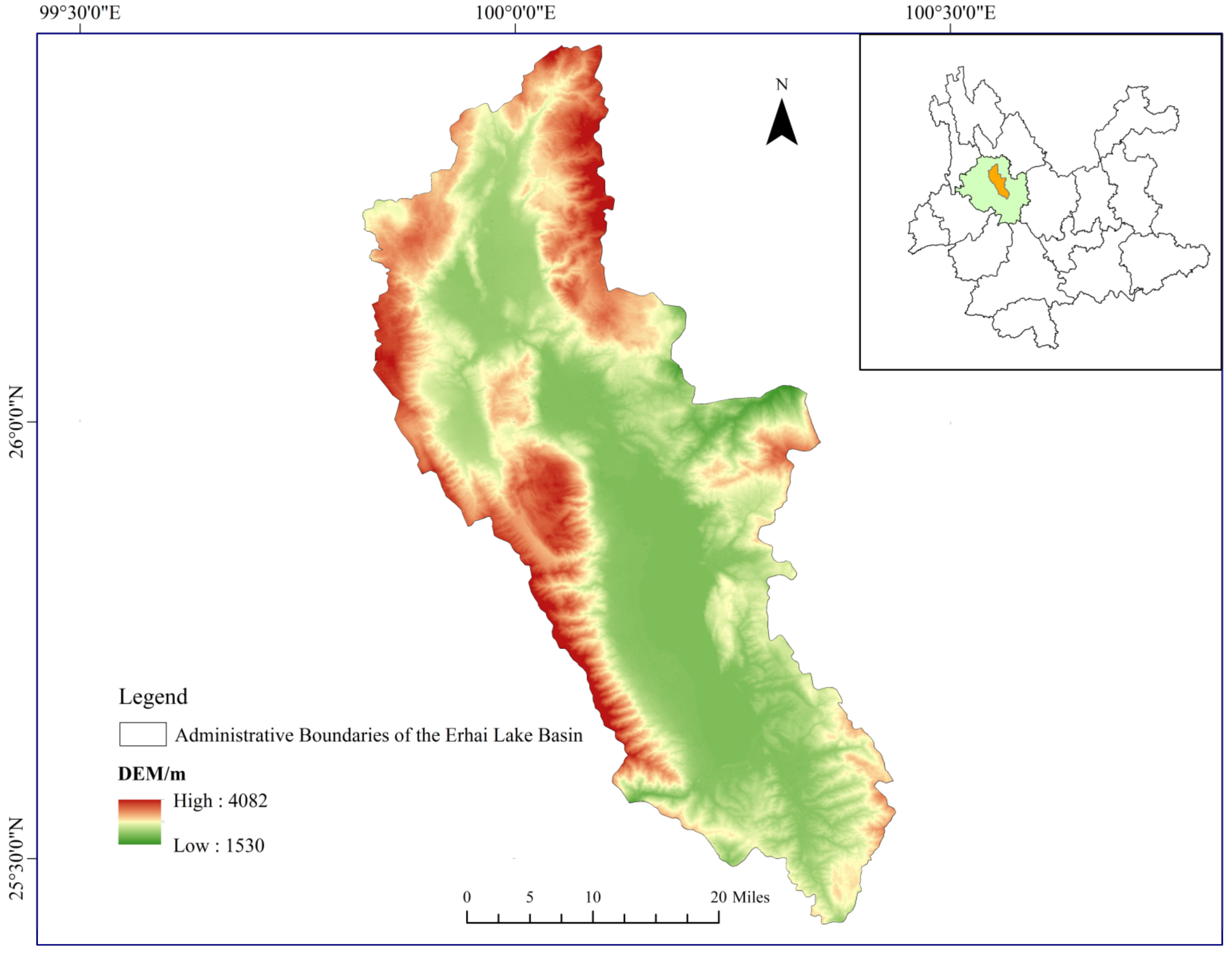
2.1. Study Area

Erhai Lake is the seventh-largest freshwater lake in China, situated on the Yunnan Plateau in the southwestern part of the country. It belongs to the southern end of the Hengduan Mountains, spanning from approximately 100°05′ to 100°17′ east longitude and from 25°36′ to 25°58′ north latitude. The total area of the lake is 2565 km². The Erhai Lake Basin has a subtropical plateau monsoon climate, characterized by mild temperatures and a distinct seasonality that resembles spring throughout the year. The annual average temperature is 15.5 °C, and the average annual precipitation is 1000 mm. The Erhai Lake Basin, as an important garlic-producing area in Yunnan Province, has a topographical trend of high in the west and low in the east, which undoubtedly has a profound impact on the garlic planting methods, irrigation, management, and other aspects. Based on the investigation, it was found that garlic cultivation occurs in low-altitude areas of the Erhai Lake Basin, represented by the light green section in the map. At the same time, different types of land covers, such as arable land, forest land, grassland, construction land, and water areas, also have direct or indirect impacts on the growth environments and yields of garlic, as shown in Figure 1.

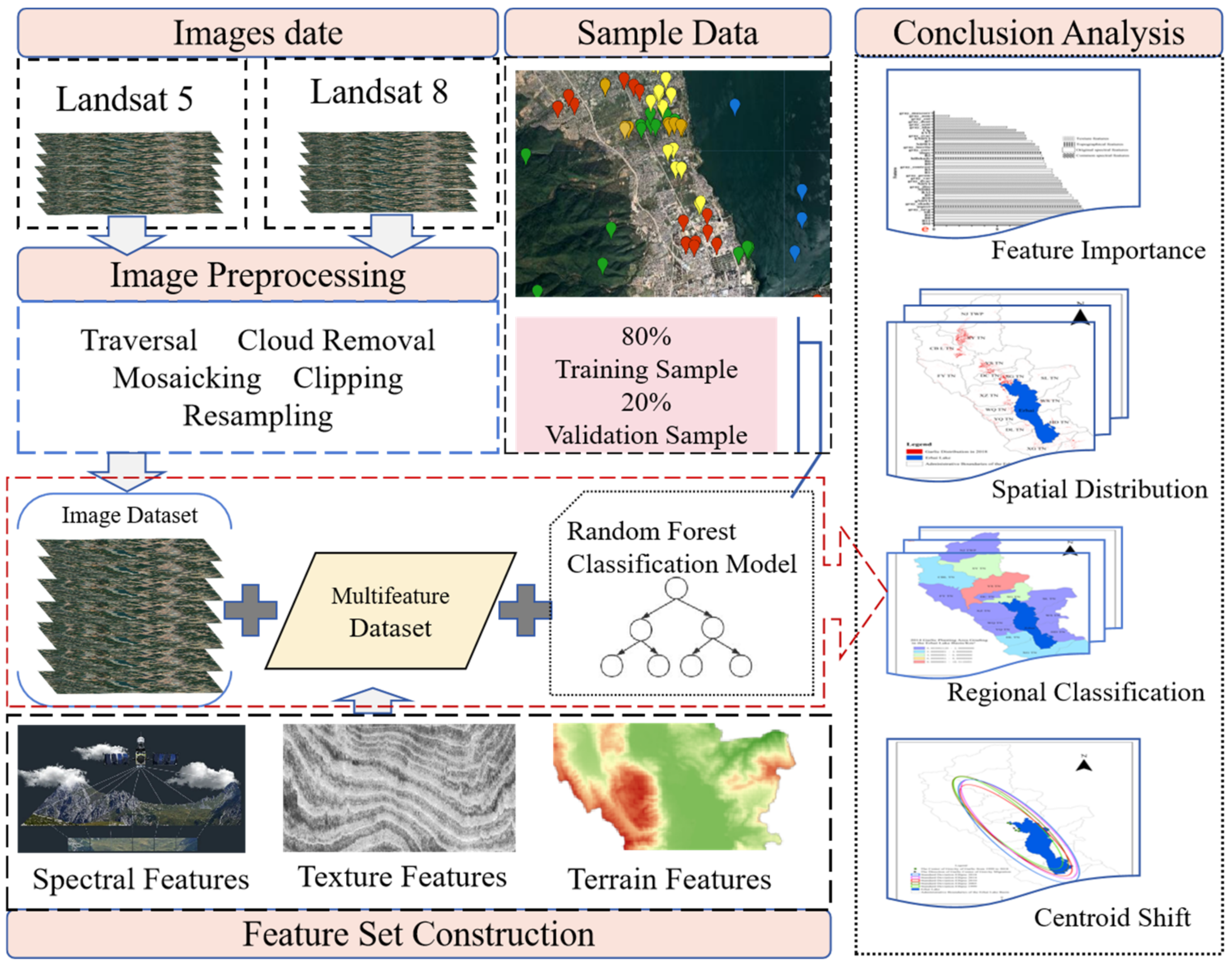
2.2. Methods

Garlic in the Erhai Lake Basin, as a geographical indication product, is one of the main sources of income for local farmers. Mapping the distribution of garlic can assist the government, farmers, and other stakeholders in better understanding the planting status and distribution of garlic, which, in turn, can facilitate the development of more effective agricultural policies, management measures, and market strategies. Initially, the image data are synthesized with the minimum cloud coverage, cropped, and resampled to the same resolution. Subsequently, terrain features and texture features are extracted by combining DEM data with the gray-level co-occurrence matrix algorithm. Finally, band synthesis is conducted to form a new remote sensing image.

This study analyzes the importance of the spectral, texture, and terrain features in crop identification. The multidimensional features were determined, the optimal features were selected, and the random forest algorithm was used to classify crops from 1999 to 2023. Then, the classification accuracy was evaluated using verification samples and statistical data, and the spatiotemporal changes in the garlic crops were analyzed, as shown in Figure 2.

2.3. Data Acquisition and Preprocessing

2.3.1. Image Data

This study was based on the Landsat 5 and Landsat 8 satellite image datasets provided by GEE. Image collections were created based on the planting and maturity time of the garlic, selecting images for the periods of 1999, 2005, 2010, 2014, 2018, and from January to February 2023. First, cloud and shadow pixels were masked using the Quality Assessment (QA) band. Cloud and shadow bits were identified by defining specific bit masks (cloudShadowBitMask and cloudsBitMask), and then these masks were applied to the QA band through bitwise operations to recognize and mask cloud and shadow pixels. Atmospheric correction and radiometric calibration were applied to the data. Images with a cloud coverage of no more than 30% were selected, followed by cropping and cloud removal operations. These steps aim to provide high-quality and accurate surface reflectance and radiance information for garlic identification.

The dataset consists of a total of 11 spectral bands. Bands B1–B9 were provided by the OLI sensor with a resolution of 30 m, whereas the panchromatic band (Band 8) has a resolution of 15 m and a swath width of 185 km. Bands B10 and B11 were provided by the TIRS sensor with a resolution of 100 m. It is worth noting that the information on the spectral bands is valid only for Landsat 8 and not for Landsat 5. To enhance the accuracy and coherence of the data, the image resolution is resampled to 30 m by defining the resampling function “var resampleImage = function(image) {…}”.

2.3.2. DEM Data

The Shuttle Radar Topography Mission Digital Elevation Model (SRTM DEM) is a DEM dataset jointly measured by the National Aeronautics and Space Administration (NASA) and the National Geospatial-Intelligence Agency (NGA), with a spatial resolution of 30 m. It is used to generate terrain parameters, including the elevation, slope, aspect, hill shade, elevation profile, and others.

2.3.3. Sample Data

Field surveys were conducted on the main garlic land cover types during the ripening period from January to February in the Erhai Lake Basin. Through visual interpretation and on-site investigation, areas with similar regional colors and texture features were marked as garlic and other crops. The annual sample point numbers and their classifications are shown in

Table 1. The number of sample points in the Erhai Lake Basin from 1999 to 2023.

Year	Garlic	Water	Construction Land	Woodland	Green House	Not Garlic	Grassland
1999	302	105	100	140	100	100	43
2005	307	102	105	143	100	100	40
2010	300	100	110	145	100	105	45
2014	306	104	105	140	100	100	47
2018	310	100	110	145	100	110	45
2023	305	100	110	140	100	103	46

. The sample collection work was carried out using the GEE cloud platform. In the Erhai Lake Basin, characterized by Cangshan Mountain and Erhai Lake, the land cover types can be divided into seven categories, taking 2018 as an example: construction land; garlic cultivation areas; greenhouses; non-garlic areas; water; forests; and grasslands. Among them, the built-up areas include 110 samples of houses, roads, factories, and mines. The non-garlic areas encompass 110 samples of cultivated land, succulent planting, flower planting, etc., excluding garlic and greenhouses. Additionally, there are 310 garlic samples, 100 waterbody samples, 145 forest samples, 100 greenhouse samples, and 45 grassland samples, totaling 920 sample points. To ensure an adequate number of validation samples for assessing the model’s performance and addressing overfitting issues, the training and validation ratio was set at 8:2. Splitting the dataset into training and testing sets and repeating the process multiple times for evaluation enable the assessment of model performance and consistency verification.

2.4. Feature Extraction

2.4.1. Feature Set Construction

The study area’s vegetation cover types, terrain characteristics, and vegetation maturity period guided the selection of features for garlic identification. Using Landsat 8 imagery, the calculations yielded 40 features comprising spectral indices, terrain characteristics, and texture features. These features, previously utilized in the land-use classification, were chosen based on their relevance to garlic identification [13]. The details of these features are provided in

Table 2. Characteristic variables and their calculation formulas.

Acronym	Formula
NDVI	(NIR − RED)/(NIR + RED)
NDWI	(Green − NIR) −/− (Green + NIR)
NDBI	(SWIR2 − NIR) −/− (SWIR2 + NIR)
BSI	((RED + SWIR1) − (NIR + BLUE)) −/− ((RED + SWIR1) + (NIR + BLUE))
BAI	(BLUE − NIR) −/− (NIR + BLUE)
g NDVI	(NIR − Green) −/− (NIR + Green)
EVI	2.5 * ((NIR − RED) −/− (NIR + 6 * RED − 7.5 * BLUE + 1))
SR	NIR −/− RED
Clg	(NIR/Green)/−1
kNDVI	Tanh(NDVI2)

, along with the original spectral features (B1–B11). These features include the Normalized Difference Vegetation Index (NDVI), Normalized Water Index (NDWI), Normalized Built-up Index (NDBI), Bare Soil Index (BSI), Enhanced Vegetation Index (EVI), and Spectral Ratio (SR). Different from sensors such as Sentinel, the dataset from Landsat 8 does not include the red-edge band and related vegetation indices mentioned by YOU et al. [14] during feature selection. When extracting texture features from the images, we used the gray-level co-occurrence matrix to compute the following 16 features: the entropy (ENT); inverse difference moment (IDM); angular second moment (ASM); variance (VAR); contrast (CONTRAST); correlation (CORR); dissimilarity (DISS); sum average (SAVG); shade (SHADE); difference variance (DVAR); profile (PROM); inertia (INTERTIA); sum variance (SVAR); spectral entropy (SENT); direction entropy (DENT); and maximum correlation (MAXCORR). To prevent overfitting and computational redundancy, only three terrain features were selected: slope (Slope), aspect (Aspect), and hill shade (Hill Shade).

2.4.2. Gray-Level Co-Occurrence Matrix (GLCM) Algorithm

The gray-level co-occurrence matrix (GLCM) is a statistical tool that is used to describe the texture features of digital images. The GLCM finds wide application in various fields, such as image processing, computer vision, and remote sensing image analysis. The gray-level co-occurrence matrix is based on the spatial relationships among the grayscale values in an image, capturing the statistical relationships between the pixel grayscale values in the image texture. In this study, the “glcm Texture()” function was utilized in GEE to calculate the texture features. The parameter “size” for the co-occurrence matrix’s neighborhood size was set to 1, and the “kernel” for calculating the offset of the center pixel was set to the default neighborhood kernel. Afterward, through the “gray.unitScale(0, 0.30)” operation, the pixel values of the grayscale image were normalized, bringing them within the range of 0–0.30. Following this, the “multiply” operation was applied to multiply the pixel values by 100, scaling the values to within the range of 0–30. Finally, the “toInt()” operation was used to convert the pixel values to the integer type.

In the calculation of the grayscale image, the original color composite image was created by linearly combining the red (R), green (G), and near-infrared (NIR) bands of the composite image with specific weights: 0.3, 0.59, and 0.11, respectively [15]. This linear combination is commonly used for extracting texture features after converting a color image to a grayscale image. The formula is as follows:

$$Gray=({0.3}^{\ast }NIR)+({0.59}^{\ast }R)+({0.11}^{\ast }G)$$

where INR is the near-infrared light, R is the infrared light, and G is the green light.

2.4.3. Random Forest Algorithm and Feature Selection

Leo Breiman introduced the random forest algorithm in his 2001 paper, “Random Forests” [16]. The random forest algorithm is an ensemble learning algorithm that consists of multiple decision trees. Multiple decision trees are created by performing random, with-replacement sampling on the training data (bootstrap sampling). Additionally, random feature selection is applied to each decision tree, enhancing the model’s diversity and generalization capability. Randomly selecting a subset of features at each node of every decision tree ensures that each tree is distinct, which thereby enhances the diversity of the random forest. This prevents certain features from dominating the model’s predictions. In this study, we applied the random forest algorithm to classify Landsat 5 and 8 images. In GEE, the advanced random forest classifiers can be constructed using the “ee.Classifier.randomForest()” and “ee.Classifier.smileRandomForest()” functions. These functions train and predict models by configuring the hyperparameters such as the number of decision trees, the method of feature selection, the maximum depth of the decision trees, and other relevant parameters. The selected number of decision trees for classification is 1000. The RMSE plot for decision trees is provided in Supplementary Figure S2. In this study, in addition to determining the number of decision trees, it was necessary to set five parameters for each branch: the number of variables per branch; the minimum leaf size; the input fraction per tree; the maximum number of leaf nodes; and the seed number. The number of variables per branch was set to have no limit on the number of variables for the sub-tree. The minimum leaf size represents the number of terminal nodes, which was set to 1 in this case, without limiting the number of leaf nodes for the decision trees. The input fraction per tree represents the proportion of the input to the bag for each tree, which was set to 0.5 in this case. The maximum number of leaf nodes was set to unlimited. The seed number represents the seeds used in the random number generator, a pseudorandom number, set to the default value (“Default”). Relevant studies have found that the classification performance may deteriorate after adding a certain number of feature variables [17,18]. To address issues such as overfitting due to excessive variables and poor classification performance caused by computational complexity, the random forest algorithm automatically leverages out-of-bag (OOB) data. The algorithm utilizes internal functions to perform importance ranking and selects the top-ranked features for classification, thereby achieving the optimal classification performance.

2.4.4. Accuracy Assessment

In GEE, the sample points are integrated into a test set named “Test” to compute the confusion matrix of the classifier. Subsequently, relevant metrics related to the classification performance are outputted. The confusion matrix is employed to assess the performance of the classifier, illustrating the correct and incorrect classifications on the test set to validate the classification accuracy. To evaluate the performance of the classifier, various evaluation metrics such as the consumer accuracy (CA), producer accuracy (PA), overall accuracy (OA), and Kappa coefficient are computed. The consumer accuracy (CA) represents the proportion of correctly classified samples by the classifier among all true samples, the producer accuracy (PA) represents the proportion of samples that actually belong to a certain class among all the samples that the classifier predicts to be of that class, and the overall accuracy (OA) represents the proportion of correctly classified samples over the entire test set. The Kappa coefficient, a crucial metric for assessing the overall performance of the classifier, is a measure of the consistency between the classifier and random classification. It accurately assesses the performance of the classifier in handling class imbalances and random predictions.

3. Results and Analysis

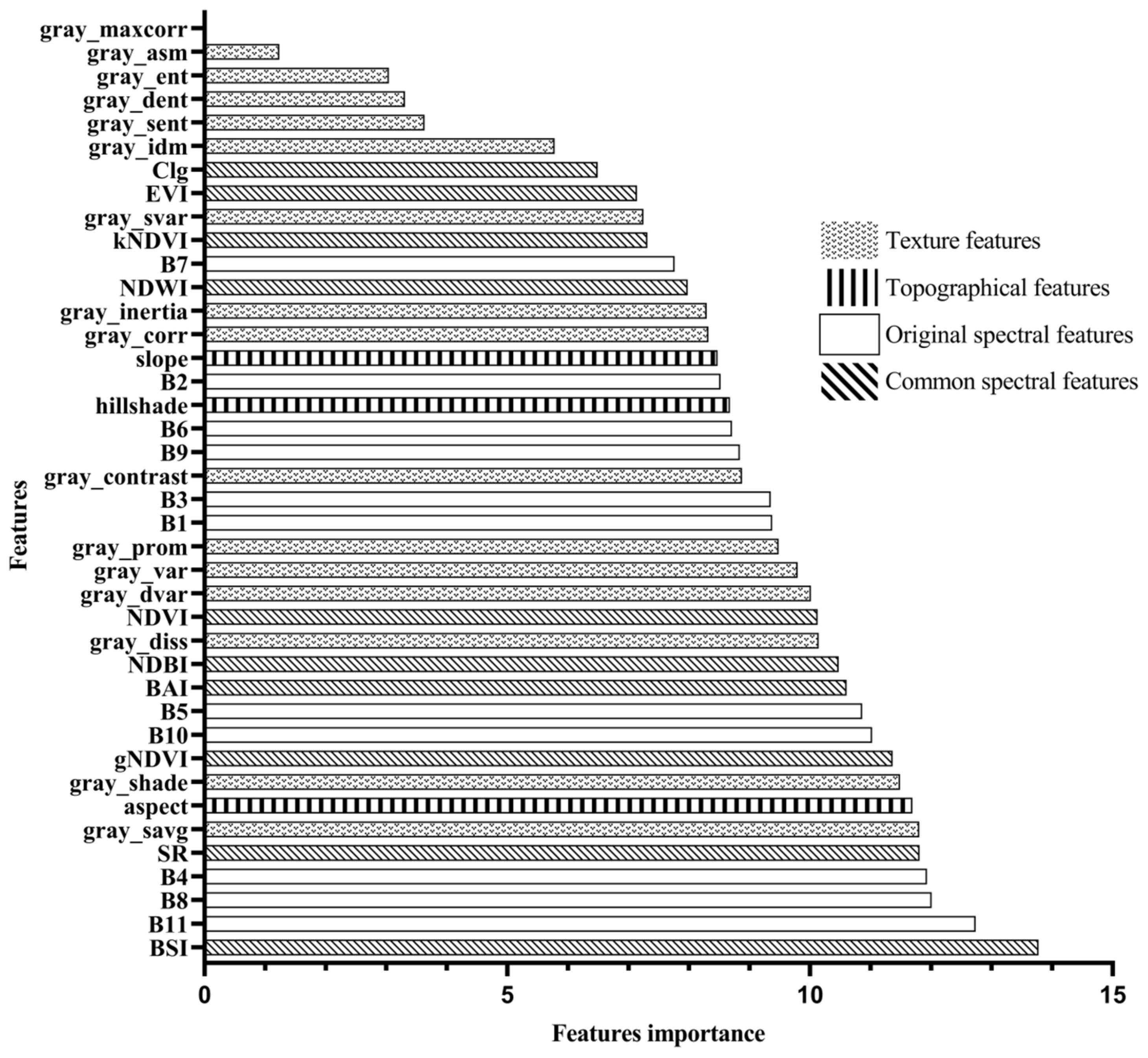
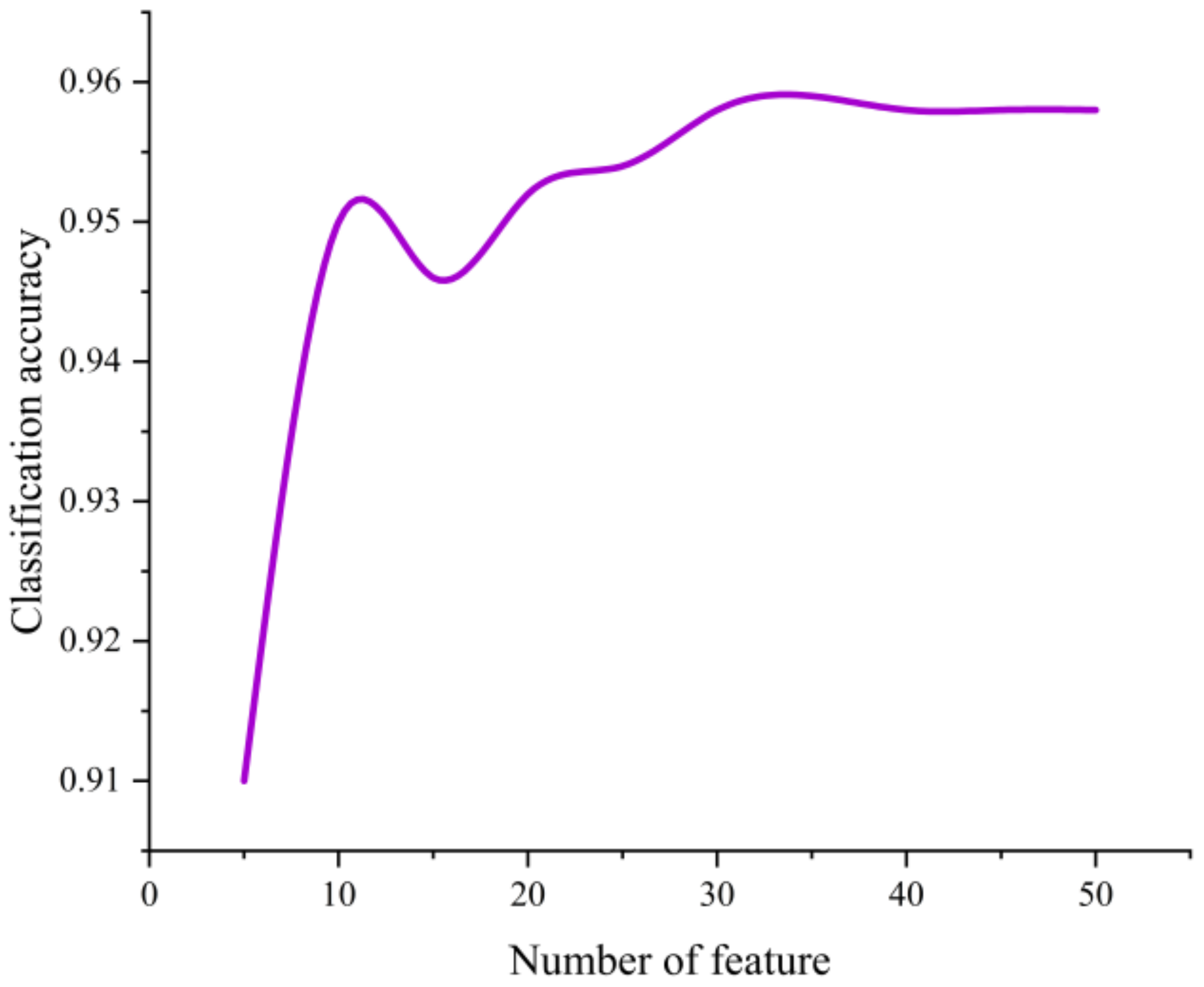
3.1. Feature Selection Analysis

Based on the remote sensing imagery of the Erhai Lake Basin in 2018, this study selected 40 feature variables. The random forest algorithm was then applied to rank the importance of each of these feature variables, and the results are presented in Figure 3. Figure 3 visually indicates that the importance of each feature variable is concentrated between 0% and 14%. Ordinary spectral features and raw spectral features are among the most important for land-use classification.

Among the texture features, the gray_savg band has the highest importance, reaching up to 11.81%. In contrast, the second-order moments of angles (gray_amxcorr) do not play a role in land-use classification. The BSI (Bare Soil Index) contributes the most to the ordinary spectral indices, reaching up to 13.75%. Among the terrain features, the aspect contributes the most, reaching up to 11.69%. Among the texture features, gray_maxcorr, gray_sent, gray_dent, gray_ent, and gray_asm have the least impact on the classification. Out of the 40 feature variables, 16 features have importance rankings of 10% or higher in the classification. Of course, like Kolluru V and others, we can also demonstrate how each variable helps predict the garlic distribution by plotting response curves [19]. Please refer to Supplementary Figure S1 for the variable importance for other years.

According to the relationship between the number of classification features and the classification accuracy, as shown in Figure 4, with the increase in the number of features, the classification accuracy initially rose and then decreased, which was followed by another increase before it gradually leveled off. The stability of the classification accuracy exhibited fluctuations with the number of features in the range of 10–30. As the number of features increased from 5 to 10, the classification accuracy increased from 0.910 to 0.950. However, after the number of features reached 35, the classification accuracy did not show a consistent increase but fluctuated with the increasing number of features. When the number of features reached 35, the classification accuracy peaked at 0.959. As the number of classification features exceeded 45, the accuracy gradually leveled off and stabilized at 0.958. Considering that the increase in the number of features could reduce computational efficiency, the top 35 features of importance were used. This included 11 original spectral features (B11; B8; B4; B10; B5; B1; B3; B9; B6; B2; B7), 10 spectral index features (BSI; SR; gNDVI; BAI; NDBI; NDVI; NDWI; kNDVI; EVI; Clg), 11 texture features (gray_savg; gray_shade; gray_diss; gray_dvar; gray_var; gray_prom; gray_corr; gray_intertia; gray_svar; gray_idm; gray_contrast), and 3 terrain features (aspect; hillshade; slope).

3.2. Accuracy Analysis

The confusion matrix, based on the 2018 classified data with feature selection, is presented in

Table 3. Confusion matrix for feature selection.

	Garlic	Waterbody	Construction Land	Woodland	Greenhouse	Not Garlic	Grassland
Garlic	235	0	2	0	0	0	0
Water	0	79	0	0	0	0	0
Construction land	4	0	82	0	1	2	1
Woodland	0	0	1	121	0	1	0
Green house	3	0	0	0	71	4	0
Not garlic	1	0	0	1	6	83	2
Grassland	0	1	0	0	0	1	34
Producer accuracy (%)	99.16	100.0	91.11	98.37	91.03	89.25	94.44
User accuracy (%)	96.71	98.75	96.47	99.18	91.02	91.21	91.89

Note: A total of 235 “Garlic” samples were correctly classified as “Garlic”, 4 “Construction land” samples were misclassified as “Garlic”, 99.16% of the samples that were actually garlic were correctly classified, and 96.71% of the samples predicted as “Garlic” by the model were indeed garlic.

. The overall accuracy is 95.79%, and the Kappa coefficient is 0.95. The user accuracy for each land-class classification is consistently above 90%. The producer accuracy, garlic, waterbodies, built-up areas, forests, greenhouses, and grasslands exhibit accuracies exceeding 90%. However, the producer accuracy for the non-garlic land class is relatively lower at 89.25%. The lower accuracy for the non-garlic land class is mainly attributed to the inclusion of cultivated land other than garlic and greenhouses, such as areas with succulent plants, flower cultivation areas, etc. During the collection of the sample points, the accurate classification of these specific land uses might not have been conducted. The spectral similarity reflected in the remote sensing imagery leads to mutual confusion, resulting in a comparatively lower accuracy for this category. The land classes that exhibit better classification results are mainly garlic, waterbodies, and forests. Specifically, the mapping accuracy and user accuracy for garlic are 99.16% and 96.71%, respectively, meeting high classification standards. Over the past five years, both the overall accuracy and Kappa coefficient have consistently remained above 90%, demonstrating a stable and satisfactory classification level. This indicates good model performance and effective training, as depicted in Figure 5.

3.3. Classification Analysis

Following the above steps, conducting feature selection analysis, and sequentially processing remote sensing imagery data from 1999, 2005, 2010, 2014, 2018, and 2023, the garlic planting distribution in the Erhai Lake Basin over the past 20 years was obtained, and it is illustrated in Figure 6. From the figure, it can be observed that from 1999 to 2005, the main garlic planting areas were upstream of the Erhai Lake Basin and in the western region. By 2010, with the decline in garlic prices, the planting area significantly decreased and was mainly concentrated in the western and northwest areas of the Erhai Lake Basin. By 2014, influenced by policies, the garlic planting area had shifted towards the northwest regions of the Erhai Lake Basin. This trend continued until 2018, forming a minor cultivation area in the western region. The primary concentration of garlic cultivation was observed in the northern part of the Erhai Lake Basin across five townships. By 2023, there was no longer any garlic cultivation within the Erhai Lake Basin. Based on the image recognition, the garlic cultivation area in 2023 was nearly zero.

To better illustrate the garlic cultivation areas in various townships within the Erhai Lake Basin, a classification map based on remote sensing image recognition was generated to show the statistical distribution of the garlic cultivation areas. The garlic cultivation area classification maps are presented in Figure 7. Considering the development history of garlic cultivation in the Erhai Lake Basin, in 1999, garlic planting was primarily concentrated in the northern and western parts of the basin, encompassing several townships. By 2005, the garlic cultivation area had gradually expanded. Townships with garlic cultivation areas exceeding 8 km² accounted for three-eighths of the total number of townships in the Erhai Lake Basin. By 2010, inflation led to a decline in garlic prices, resulting in decreases in the garlic cultivation areas across various townships in the Erhai Lake Basin, with none exceeding 6 km². In 2014, garlic cultivation gradually rebounded, and the planting distribution gradually shifted towards the northern part of the Erhai Lake Basin, with an increasing planting area. By 2018, garlic cultivation was predominantly concentrated in the northern part of the Erhai Lake Basin. Looking at the overall picture, garlic cultivation in the Erhai Lake Basin began in the western region and then spread towards the upstream areas of the Erhai Lake Basin. Comparatively, the eastern part of the Erhai Lake Basin had the smallest garlic cultivation area. From a geographical perspective, garlic is a crop that consumes significant amounts of water and fertilizer, and it is primarily cultivated in the areas surrounding Erhai Lake, where water resources are abundant.

The center of gravity analysis method [20] and standard deviation ellipse theory [21] were employed to calculate the center of gravity and standard deviation ellipse of garlic cultivation in the Erhai Lake Basin from 1999 to 2018 (see Figure 8 and

Table 4. Standard deviation ellipse parameters for garlic in the Erhai Lake Basin from 1999 to 2018.

Year	CenterX	CenterY	XStdDist	YStdDist	Rotation	XSid/YStd
1999	100.09	25.93	0.08	0.33	152.87	4.30
2005	100.09	25.93	0.08	0.34	152.51	4.01
2010	100.12	25.89	0.08	0.32	151.92	4.21
2014	100.13	25.89	0.09	0.35	153.56	3.98
2018	100.13	25.88	0.10	0.36	154.16	3.64

Note: CenterX: the coordinate of the center of the ellipse on the X-axis; CenterY: the coordinate of the center of the ellipse on the Y-axis; XStdDist: the standard deviation along the X-axis, indicating the spread of data in the X direction.; YStdDist: the standard deviation along the Y-axis, indicating the spread of data in the Y direction; Rotation: the rotation angle of the ellipse, representing the degree of rotation relative to the original coordinate axis; and XSid/YStd: the ratio of the standard deviation along the X-axis to the standard deviation along the Y-axis, describing the shape of the ellipse.

). According to the center of gravity analysis, from 1999 to 2010, garlic cultivation in the Erhai Lake Basin expanded towards the southeast. From 2010 to 2014, the center of gravity shifted towards the northeast. Between 2014 and 2018, the direction of garlic cultivation’s center of gravity was southwest. The eastward spread of garlic cultivation’s center of gravity in the Erhai Lake Basin slowed down from 2010 to 2018, and a change in direction occurred in 2014. In the standard deviation ellipse theory, the major axis represents the directional distribution, the minor axis represents the distribution range, and the major-to-minor-axis ratio indicates the directionality of the expansion. A ratio close to 1 suggests no clear directionality. During the period from 1999 to 2018, the ratio of the major-to-minor axis consistently exceeded 2, indicating a pronounced directionality. From 1999 to 2010, the ratio of the major-to-minor axis decreased from 4.3 to 4 and then increased to 4.2. This indicates that the directional expansion of garlic cultivation strengthened initially and then weakened during this period. By 2018, the major-to-minor-axis ratio further decreased to 3.64, indicating a continued weakening of the directional expansion. Furthermore, it was observed that the minor axis of the standard deviation ellipse elongated during the period from 2005 to 2018, indicating an increase in the distribution range of garlic cultivation.

4. Discussion

In agricultural remote sensing research, most studies primarily focus on the identification of cereal crops, while there is relatively less research domestically and internationally on the remote sensing identification of economic crops such as tobacco, rubber, tea, and garlic. Currently, the research on garlic extraction primarily combines phenological periods with machine learning algorithms. For example, Wu Shuang and others obtained Sentinel-2 remote sensing images covering the entire growth cycle of garlic. They made progress in garlic identification by utilizing different combinations of multiple temporal phases [22]. Additionally, some studies used convolutional neural networks to create garlic land classification models based on the growth stages. Through the use of high-resolution images and deep learning, they were able to detect the garlic yield throughout the entire growth stage [23].

In terms of classification methods, Indonesian scholars chose the k-nearest neighbor and maximum likelihood classification methods and compared them with pixel-based and image-based garlic classification results from previous studies, finding that the k-nearest neighbor classification method yields better classification results compared to support vector machine and maximum likelihood classification [24]. Based on the random forest algorithm and the object-oriented approach, Ma Zhanlin and colleagues added index features and utilized simple non-iterative clustering (SINC) to select the optimal segmentation scale for garlic extraction. The overall accuracy and Kappa coefficient reached 94.54% and 0.93, respectively. This achievement is consistent with the good classification results by Tian Haifeng and others in identifying garlic and winter wheat using active and passive remote sensing [25]. However, the research on garlic is mainly concentrated in northeastern China, such as in Shandong, and there is almost no research on the identification of garlic in Yunnan. This study utilized Landsat satellite imagery on the GEE platform for garlic identification in the Erhai Lake Basin. This approach significantly reduces data acquisition and preprocessing efforts. The classification performance was improved compared to those of previous studies. The overall accuracy was improved by approximately 1.3%, and the Kappa coefficient increased by around 2%. In addition to supplementing the literature references related to garlic in the Erhai Lake Basin, this study validates the applicability of feature selection combined with a random forest classification model based on the GEE platform for garlic determination.

In most articles related to feature selection, spectral features and vegetation index features play a dominant role. Spectral indices such as B8 and B11 hold higher positions in the feature importance ranking, followed by texture features, and lastly, red-edge spectral indices [26,27,28]. There are fewer articles in the literature that simultaneously incorporate texture features and terrain features in feature selection studies using Landsat imagery. However, related studies indicate that texture features, along with terrain features, play an important role in land-use classification [29]. The response to texture features becomes more pronounced as the land-use types become more complex [30]. In this study, four terrain features exhibited high correlation, which could impact the classification results. Therefore, only a subset of terrain features was included in the analysis. Considering interference from noise and other factors, a combination of median and Gaussian filtering was employed for elimination. Additionally, the kNDVI, which is better at handling noise, enhancing saturation, and reducing “background effects” (such as soil, sparse vegetation, and water) [31], was added. This approach effectively addresses the saturation mixing pixel issue encountered by traditional indices. The kNDVI plays a role in improving the quantification and understanding of photosynthesis on a global scale going beyond the scope of vegetation monitoring, including applications in change and anomaly detection, phenology, and greening studies, among others. This study also found that the kNDVI exhibits stronger stability and robustness under various environmental conditions, such as dense forests, grasslands, and mixed forests, compared to the traditional NDVI and NIRv [32,33]. In the classification conducted in this study, the kNDVI played a significant role, with a feature importance of 7.314%. However, its importance was relatively lower than that of the NDVI.

5. Conclusions

This study, leveraging the powerful data processing and computational capabilities of Google Earth Engine (GEE), utilized Landsat 5 and Landsat 8 satellite imagery as remote sensing data. By employing feature selection and the random forest (RF) algorithm, this study achieved the extraction of the spatial distribution information for garlic in the Erhai Lake Basin. Subsequently, the center of gravity analysis and the standard deviation ellipse theory were utilized to analyze the spatiotemporal evolution patterns of the garlic. The main conclusions are as follows:

(1)

In the land-use classification of the Erhai Lake Basin, the random forest algorithm selected feature bands with the following importance ranking: spectral features > vegetation features > texture features > terrain features. Through feature selection analysis, the number of features was reduced from 40 to 35. Having too many features can burden the model, making it prone to overfitting and decreasing the accuracy.

(2)

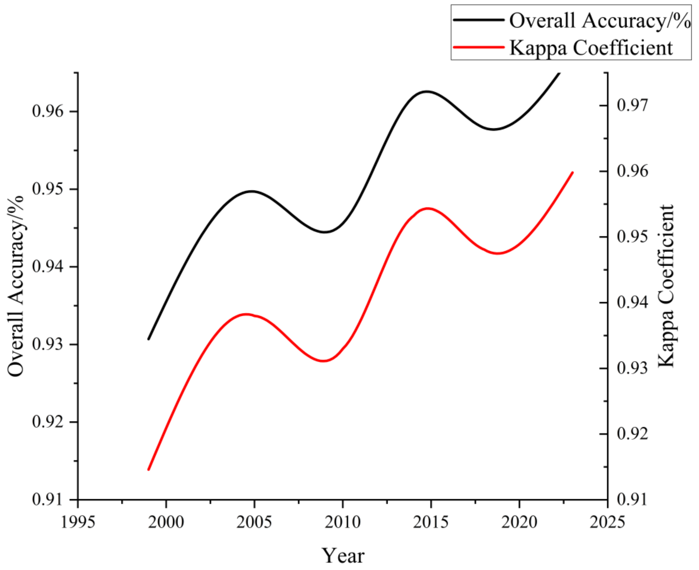
The random forest method based on feature selection achieved high accuracy in the land-use classification in the Erhai Lake Basin, Yunnan Province. The overall classification accuracy reached 95.79%, with a Kappa coefficient of 0.95. Specifically, the garlic mapping accuracy reached 99.16%, and the user accuracy reached 96.71%. The land-use classification accuracy from 1999 to 2018 consistently exceeded 93%, meeting the good classification standard.

(3)

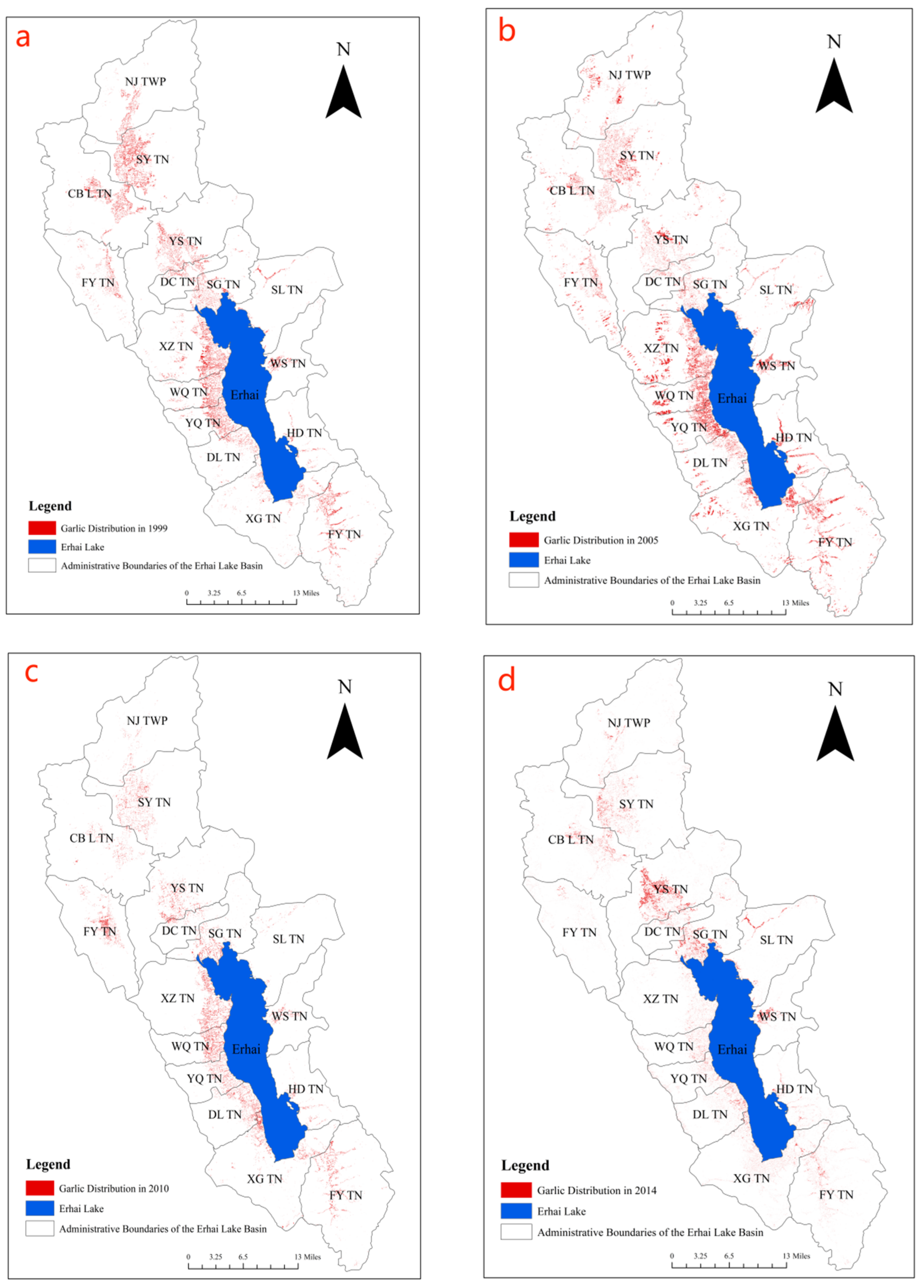
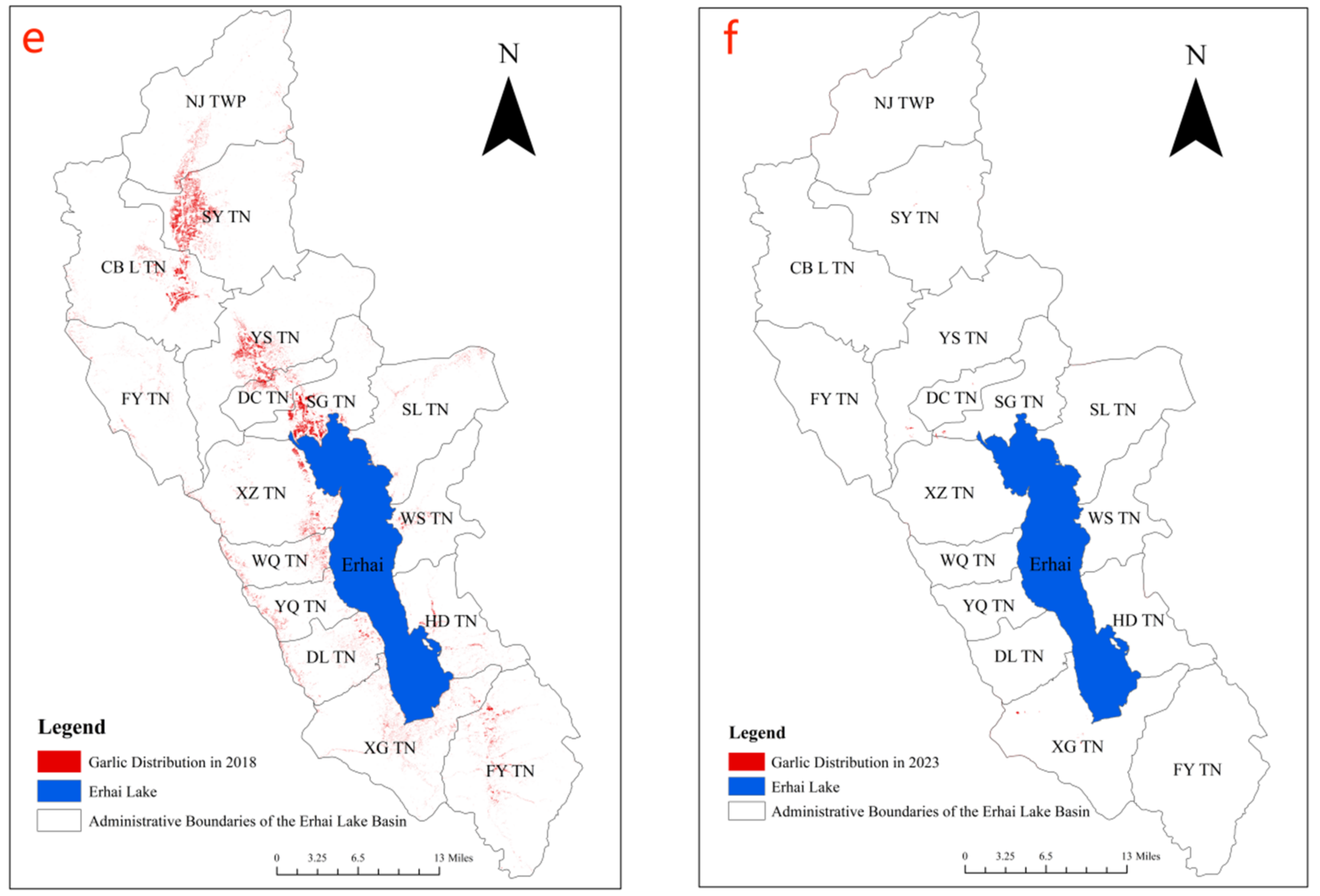
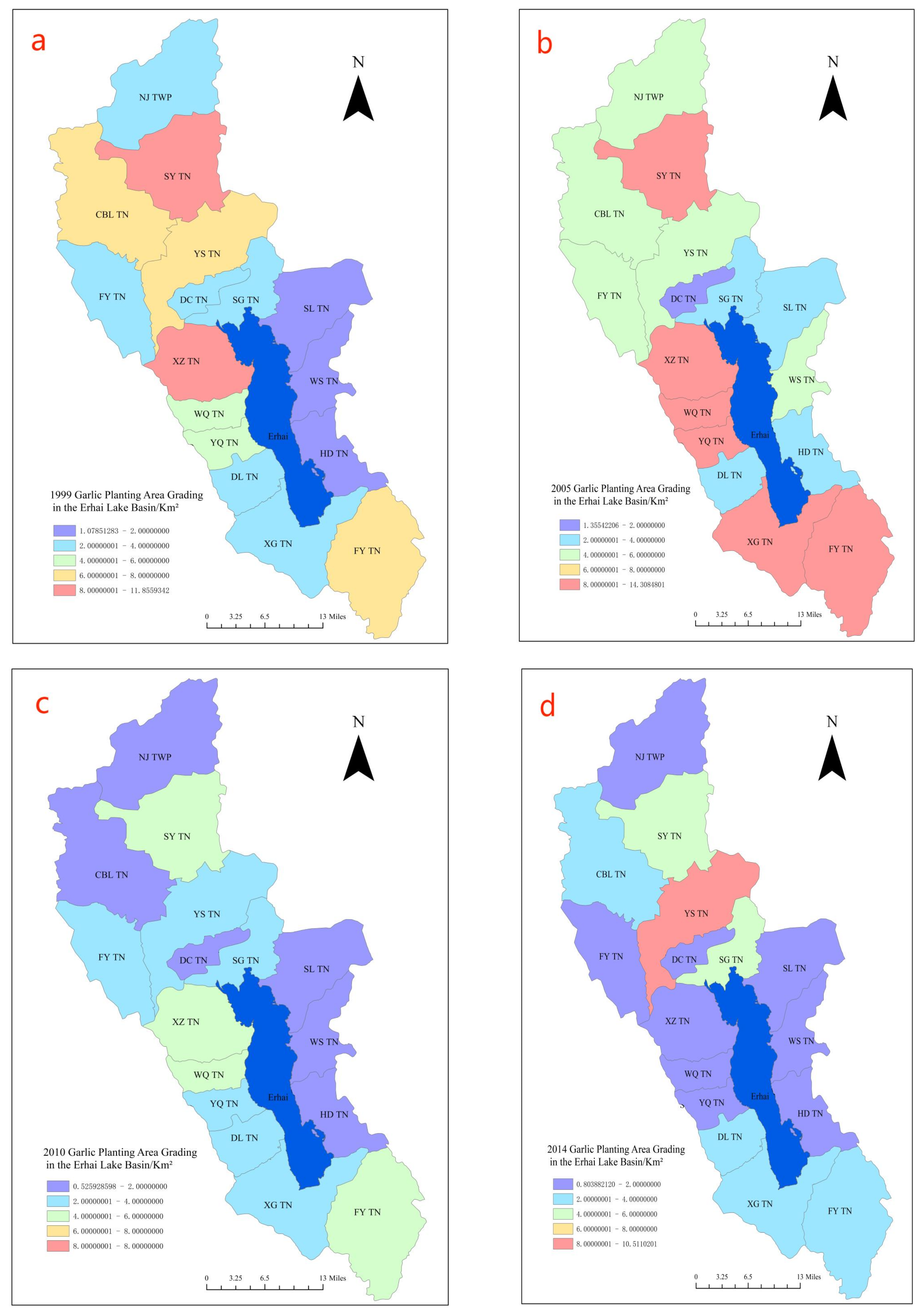
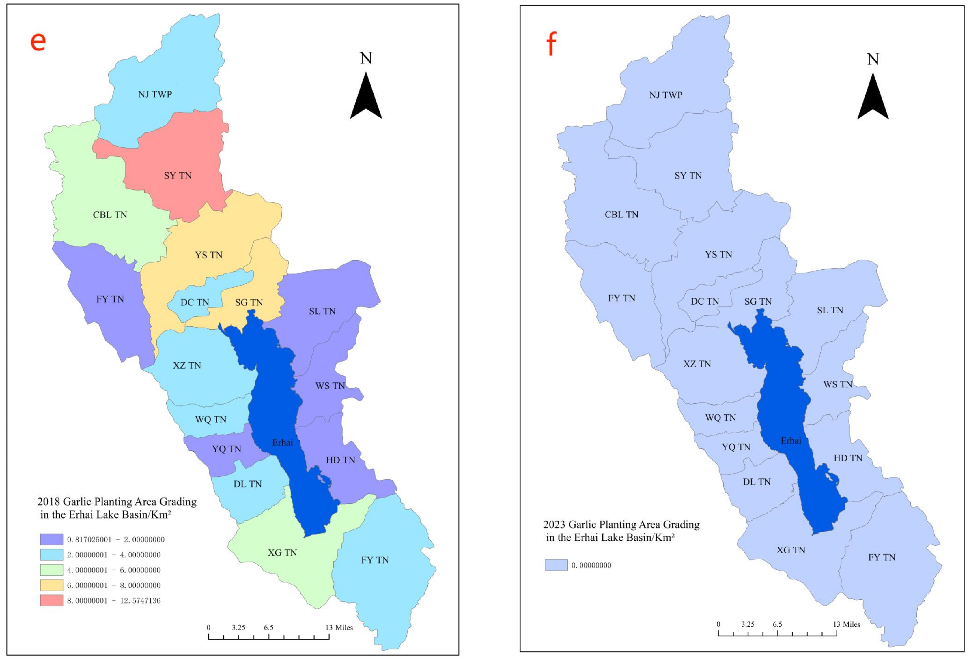
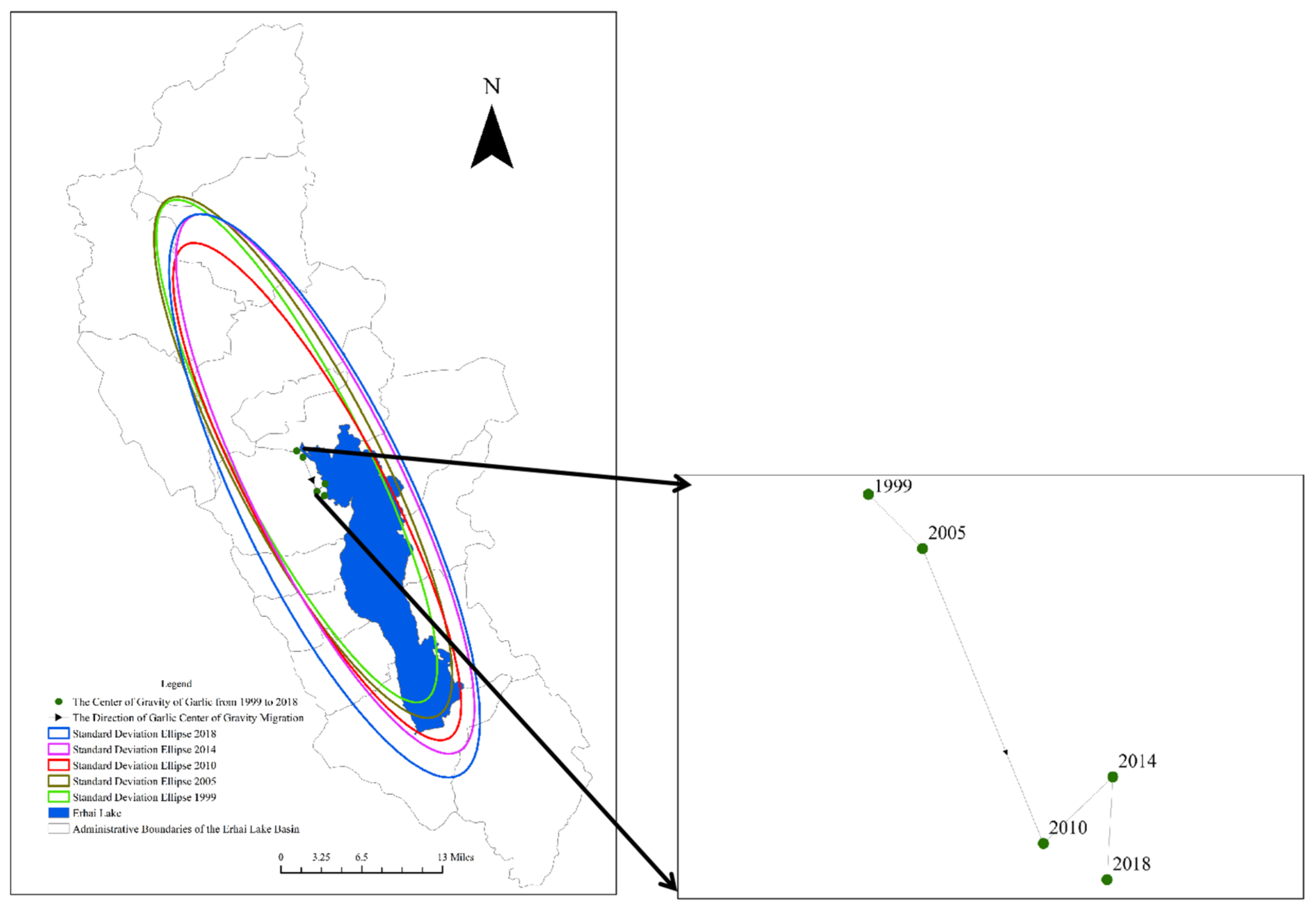
The expansion directionality of the garlic cultivation in the Erhai Lake Basin increased first and then decreased from 1999 to 2018. From 2005 to 2018, garlic cultivation showed a saturation trend in the longitudinal direction, slowly exhibiting a trend of lateral development. Over the past 20 years, the center of garlic cultivation has gradually shifted in the southeast direction, and garlic cultivation in various towns in the Erhai Lake Basin has gradually shifted from a relatively even distribution to a concentration in the upstream region of the Erhai Lake Basin.

Considering the interference that may occur when applying the pixel-based crop extraction and classification methods, such as “salt-and-pepper artifacts” and “salt-and-pepper noise”, this study employed a combination of median filtering and Gaussian filtering to eliminate the interference, with the aim of enhancing the classification accuracy. Additionally, the incorporation of the kNDVI was introduced to better handle the noise and reduce the impact of the interference on the classification results, thereby improving the accuracy to a certain extent.

References

- Weiss, M.; Jacob, F.; Duveiller, G. Remote sensing for agricultural applications: A meta-review. Remote Sens. Environ. 2020, 236, 111402. [Google Scholar] [CrossRef]
- Pan, H.; Chen, Z.; Ren, J.; Li, H.; Wu, S. Modeling winter wheat leaf area index and canopy water content with three different approaches using Sentinel-2 multispectral instrument data. IEEE J. Stars 2018, 12, 482–492. [Google Scholar] [CrossRef]
- Zhang, L.; Liu, Z.; Ren, T.W.; Liu, D.; Ma, Z.; Tong, L.; Zhang, C.; Zhou, T.; Zhang, X.; Li, S. Identification of seed maize fields with high spatial resolution and multiple spectral remote sensing using random forest classifier. Remote Sens. 2020, 12, 362. [Google Scholar] [CrossRef]
- Zhao, Y.Y.; Feng, D.L.; Jayaraman, D.; Belay, D.; Sebrala, H.; Ngugi, J.; Maina, E.; Akombo, R.; Otuoma, J.; Mutyaba, J.; et al. Bamboo mapping of Ethiopia, Kenya and Uganda for the year 2016 using multi-temporal Landsat imagery. Int. J. Appl. Earth Obs. Geoinf. 2018, 66, 116–125. [Google Scholar] [CrossRef]
- Li, F.; Ren, J.; Wu, S.; Zhang, N.; Zhao, H. Effects of NDVI time series similarity on the mapping accuracy controlled by the total planting area of winter wheat. Trans. Chin. Soc. Agric. Eng. 2021, 37, 127–239. [Google Scholar]
- Qiu, B.; Li, W.; Tang, Z.; Chen, C.; Qi, W. Mapping paddy rice areas based on vegetation phenology and surface moisture conditions. Ecol. Indic. 2015, 56, 79–86. [Google Scholar] [CrossRef]
- Chen, J.; Chen, J.; Liao, A.P.; Cao, X.; Chen, L.; Chen, X.; He, C.; Han, G.; Peng, S.; Lu, M.; et al. Global land cover map-ping at 30 m resolution: A POK-based operational approach. ISPRS J. Photogramm. Remote Sens. 2015, 103, 7–27. [Google Scholar] [CrossRef]
- Wessel, M.; Brandmeier, M.; Tiede, D. Evaluation of different machine learning algorithms for scalable classification of tree types and tree species based on Sentinel-2 Data. Remote Sens. 2018, 10, 1419. [Google Scholar] [CrossRef]
- Varin, M.; Chalghaf, B.; Joanisse, G. Object-based approach using very high spatial resolution 16-band Worldview-3 and LIDAR data for tree species classification in a broadleaf forest in Quebec, Canada. Remote Sens. 2020, 12, 3092. [Google Scholar] [CrossRef]
- Dong, J.; Xiao, X.; Menarguez, M.A.; Zhang, G.; Qin, Y.; Thau, D.; Biradar, C.; Moore, B., III. Mapping paddy rice planting area in northeastern Asia with Landsat 8 images, phenology-based algorithm and Google Earth Engine. Remote Sens. Environ. 2016, 185, 142–154. [Google Scholar] [CrossRef]
- Heng, Y.; Yu, L.; Cracknell, A.P.; Gong, P. Oil palm mapping using Landsat and PALSAR: A case study in Malaysia. Int. J. Remote Sens. 2016, 37, 5431–5442. [Google Scholar]
- Xu, W.Y.; Sun, R.; Jin, Z.F. Extracting tea plantations based on ZY- 3 satellite data. Trans. Chin. Soc. Agric. Eng. 2016, 32, 161–168. [Google Scholar]
- Ma, Z.; Xue, H.; Liu, C. Identification of garlic based on active and passive remote sensing data and object-oriented technology. Trans. Chin. Soc. Agric. Eng. 2022, 38, 210–222. [Google Scholar]
- You, H.T.; Huang, Y.W.; Qin, Z.G.; Chen, J.; Liu, Y. Forest Tree Species Classification based on Sentinel-2 images and auxiliary data. Forests 2022, 13, 1416. [Google Scholar] [CrossRef]
- Tassi, A.; Vizzari, M. Object-orientied LULC classification in Google earth engine combining SNIC, GLCM, and machine learning algorithms. Remote Sens. 2020, 12, 3776. [Google Scholar] [CrossRef]
- Breiman, L. Random Forests. Mach. Learn. 2001, 45, 5–32. [Google Scholar] [CrossRef]
- Stromann, O.; Nascetti, A.; Yousif, O.; Ban, Y. Di-mensionality reduction and feature selection for object-based land cover classification based on Sentinel-1 and Sentinel-2 time series using Google Earth Engine. Romote Sens. 2019, 12, 76. [Google Scholar] [CrossRef]
- Mitzer, M.; Atzberger, C.; Koukal, T. Treespecies classification with random forest using very high spatial resolution 8—Band World View—2 satellite data. Remote Sens. 2012, 4, 2661–2693. [Google Scholar] [CrossRef]
- Kolluru, V.; John, R.; Saraf, S.; Chen, J.; Hankerson, B.; Robinson, S.; Kussainova, M.; Jain, K. Gridded livestock density database and spatial trends for Kazakhstan. Sci. Data 2023, 10, 839. [Google Scholar] [CrossRef]
- Wang, J.Y.; Liu, Y.S. The changes of grain output center of gravity and its driving forces in China since 1990 to 2005. Resour. Sci. 2009, 31, 1188–1194. (In Chinese) [Google Scholar]
- Xiao, O.; Xiang, Z. Spatiotemporal Dynamics of Urban Land Expansion in Chinese Urban Agglomerations. Acta Geogr. Sin. 2020, 75, 571–588. [Google Scholar]
- Wu, S.; Lu, H.; Guan, H.; Chen, Y.; Qiao, D.; Deng, L. Optimal bands combination selection for extracting garlic planting area with multi-temporal sentinel-2 imagery. Sensors 2021, 21, 5556. [Google Scholar] [CrossRef] [PubMed]
- Mukhibah, D.; Imas, S.S. Classification of Garlic Land Based on Growth Phase using Convolutional Neural Network. Int. J. Adv. Comput. Sci. Appl. 2023, 14, 945–951. [Google Scholar] [CrossRef]
- Sitanggang, I.S.; Rahmani, I.A.; Caesarendra, W.; Agmalaro, M.A.; Annisa, A.; Sobir, S. Garlic Field Classification Using Machine Learning and Statistic Approaches. AgriEngineering 2023, 5, 631–645. [Google Scholar] [CrossRef]
- Tian, H.; Pei, J.; Huang, J.; Li, X.; Wang, J.; Zhou, B.; Qin, Y.; Wang, L. Garlic and winter wheat identification based on active and passive satellite imagery and the google earth engine in northern China. Remote Sens. 2020, 12, 3539. [Google Scholar] [CrossRef]
- Liu, Y.; Xiao, D.; Yang, W. An algorithm for early rice area mapping from satellite remote sensing data in southwestern Guangdong in China based on feature optimization and random Forest. Ecol. Inform. 2022, 72, 101853. [Google Scholar] [CrossRef]
- He, Y.; Huang, C.; Li, H.; Liu, Q.S.; Liu, G.H.; Zhou, Z.C.; Zhang, C.C. Land-cover classification of random forest based on Sentinel-2A image feature optimization. Resour. Sci. 2019, 41, 992–1001. [Google Scholar] [CrossRef]
- Zhang, Y.Q.; Ren, H.R. Remote sensing extraction of paddy rice in Northeast China from GF-6 images by combining feature optimization and random forest. Natl. Remote Sens. Bull. 2023, 27, 2153–2164. [Google Scholar] [CrossRef]
- Xie, Z.L.; Chen, Y.L.; Lu, D.S.; Li, G.; Chen, E. Classification of land cover, forest, and tree species classes with ZiYuan-3 multispectral and stereo data. Remote Sens. 2019, 11, 164. [Google Scholar] [CrossRef]
- Zhang, H.X.; Wangy, J.; Shang, J.L.; Liu, M.; Li, Q. Investigating the impact of classification features and classifiers on crop mapping performance in heterogeneous agricultural landscapes. Int. J. Appl. Earth Obs. Geo Inf. 2021, 102, 102388. [Google Scholar] [CrossRef]
- Camps-Valls, G.; Campos-Taberner, M.; Moreno-Martínez, Á.; Walther, S.; Duveiller, G.; Cescatti, A.; Mahecha, M.D.; Muñoz-Marí, J.; García-Haro, F.J.; Guanter, L.; et al. A unified vegetation index for quantifying the terrestrial biosphere. Sci. Adv. 2021, 7, eabc7447. [Google Scholar] [CrossRef] [PubMed]
- Wang, X.; Biederman, J.A.; Knowles, J.F.; Scott, R.L.; Turner, A.J.; Dannenberg, M.P.; Köhler, P.; Frankenberg, C.; Litvak, M.E.; Flerchinger, G.N.; et al. Satellite solar-induced chlorophyll fluorescence and near-infrared reflectance capture complementary aspects of dry-land vegetation productivity dynamics. Remote Sens. Environ. 2022, 270, 112858. [Google Scholar] [CrossRef]
- Wang, Q.; Moreno-Martínez, Á.; Muñoz-Marí, J.; Campos-Taberner, M.; Camps-Valls, G. Estimation of vegetation traits with kernel NDVI. ISPRS J. Photogramm. Remote Sens. 2023, 195, 408–417. [Google Scholar] [CrossRef]