Visible Near-Infrared Hyperspectral Soil Organic Matter Prediction Based on Combinatorial Modeling

Abstract

Non-destructive, fast, and accurate prediction of soil organic matter content in farmland is of great significance for soil fertility assessment and rational fertilization. In the process of soil organic matter prediction, it is important to give full play to the advantages of different prediction models and to integrate different prediction models to innovatively construct a combined prediction model of soil organic matter content so as to improve the prediction accuracy and generalization ability of the model. In this study, the soil organic matter content of agricultural soils was taken as the research object, and the visible near-infrared hyperspectral curves of soils were measured by the Starter Kit indoor mobile scanning platform (Headwall Photonics, Bolton, MA, USA), and the original spectral curves were firstly de-noised by Savitzky–Golay (S-G) smoothing. Secondly, the smoothed and denoised spectral data were subjected to a first-order differential transform, and the features were selected based on the first-order differential transformed spectral data using the L1-paradigm algorithm features. Then, secondly, eight algorithms based on the selected feature bands, such as LASSO Regression (LASSO) (Model 1), Multilayer Perceptron (MLP) (Model 2), Random Forest (RF) (Model 3), Gaussian Kernel Regression (GKR) (Model 4), Ridge Regression (Model 5), Long Short-Term Memory (LSTM) (Model 6), Convolutional Neural Networks (CNN) (Model 7), and Support Vector Regression (SVR) (Model 8), were applied to construct a single-prediction model of soil organic matter content. Finally, a superior linear combination-prediction model was proposed by the eight single-prediction models constructed, and the standard deviation-based prediction validity was added to test the model. The results showed the following: (1) the weights of the eight single-prediction models in the combined prediction model were ${\omega }_1^{*}=0.099$, ${\omega }_2^{*}=0.202$, ${\omega }_3^{*}=0.000$, ${\omega }_4^{*}=0.357$, ${\omega }_5^{*}=0.088$, ${\omega }_6^{*}=0.089$, ${\omega }_7^{*}=0.000$, ${\omega }_8^{*}=0.165$, respectively; (2) The average precision E of the predicted values of soil organic matter content constructed based on the eight single-prediction models was 0.856; the average standard deviation σ was 0.181, and the average prediction validity M was 0.702; (3) The accuracy E of the predicted value of soil organic matter content of the combined model was 0.893, which was 4.322% higher than the average accuracy of the single model; the standard deviation of the combined model was 0.129, which was 28.333% lower than the average standard deviation of the single model, and the prediction validity M of the combined model was 0.778, which was 10.826% higher than the average prediction validity of the single model. The combined model can be used for the effective estimation of soil organic matter content in farmland with visible near-infrared spectral data, which can provide a basis and reference for the rapid detection of soil organic matter content in farmland.

1. Introduction

Soil organic matter plays a vital role in soil health and crop growth and is a key factor in measuring soil fertility, maintaining soil ecosystem balance, and promoting sustainable agriculture [1].

When determining the organic matter content in traditional laboratories, it is often necessary to collect a large number of samples, which is destructive, costly, inefficient, discrete, etc. In the process of determining the organic matter content, it is necessary to carry out ablation treatment to destroy the complex structure of the soil and release the organic matter, and a large amount of waste liquid is generated in the process of ablation, which has a certain impact on the environment, and a large number of chemical reagents are used which pose a certain danger to the experimenter. The use of a large number of chemical reagents, to a certain degree, is harmful to the health of laboratory personnel and the environment [2].

Despite the continuous progress of IoT sensor technology, it is still difficult to accurately determine the content of soil organic matter. IoT sensors generate large amounts of real-time data, requiring powerful data processing and analysis capabilities and increasing cost and complexity. Sensors require stable communication connections with high energy and communication requirements. IoT sensors are costly to deploy and maintain and require regular calibration to ensure their accuracy, and soil organic matter data may contain sensitive information that requires appropriate encryption and security measures to protect data security and privacy [3].

The rapid development and effective application of hyperspectral technology provide favorable conditions for non-destructive, rapid, low-cost, and high spatial resolution determination of organic matter content [4]. Scholars conducted a great deal of research in the use of hyperspectral data to predict soil organic matter content, for one, by using different hyperspectral data, mainly high-resolution hyperspectral satellite/airborne data [5,6], visible, near-infrared hyperspectral data [7,8]. Secondly, due to the large number of hyperspectral data bands and the redundancy of information, there have been studies using different spectral transforms for the feature selection; spectral transforms mainly include S-G denoising, differential transforms, wavelet transforms, scattering correction, etc. [9,10,11,12], and feature selection or dimensionality reduction and other methods to screen the sensitive bands, mainly Competitive Adaptive Reweighted Sampling (CARS), Successive Projection Algorithms (SPA), Particle Swarm Optimization algorithms (PSO), Recursive Feature Elimination (RFE), Random Forest importance feature selection, PCA, and other dimensionality reduction [13,14,15,16,17,18]. Third, different prediction methods are used for the calculation of relevant parameters and model construction, mainly using a combination of various optimization algorithms and machine learning models, mainly genetic optimization, PSO, and other algorithms combined with machine learning and deep learning algorithms, such as Partial Least Squares Regression (PLSR), Random Forests (RF), Support Vector Machines (SVM), Decision Trees, Artificial Neural Network (ANN), Long Short-Term Memory (LSTM), Ridge regression, ensemble method and other machine learning and deep learning algorithms for model construction [16,17,18,19,20,21,22,23,24].

Studies have been conducted in the soil organic matter content prediction model selection mostly using a single model; each model has its advantages and disadvantages and may be affected by random factors in order to reduce the possible bias of a single model so as to obtain more accurate and stable prediction results. Researchers have explored prediction models constructed based on integrated learning methods such as Bagging, Boosting, Stacking, and fusion models constructed based on weighting methods to achieve more accurate prediction results by ensembling the advantages of different models. For example, Zhang Xiuquan et al. [16] demonstrated better accuracy in predicting soil organic matter content with a stacked generalization model constructed using four single-prediction models. Although the integrated learning model utilizes the degree of difference in structure and prediction of multiple single models, it does not consider the degree of contribution of multiple models in the integrated stacked model. Currently, common combined prediction models are constructed with the criterion that the sum of the squares of the absolute errors or the sum of the absolute values of the deviations is minimized [24], and because different time series sometimes have different magnitudes or different values that makes the sum of squares of absolute errors or the sum of absolute values of deviations not comparable. Therefore, this study proposes a combined forecasting model, which is built on the basis of multiple single forecasting models, constructs a combined model that considers the standard deviation of forecasting accuracy and takes the maximum of the constructed forecasting effectiveness model as the goal, and uses the planning and solving idea to obtain the weights of each single forecasting model, and then constructs a combined forecasting model with the weights weighted by these weights.

2. Materials and Methods

2.1. Datasets

2.1.1. Sample Collection and Measurement

Soil samples were collected from the test site, which has a warm temperate continental climate with four distinct seasons, an altitude of 776 m, an average annual temperature of 11.5 °C, an average annual rainfall of 456.7 mm, an annual sunshine hour of 2540.7 h, and a frost-free period of 176 days. The soil type of this test field is cinnamon soil, and the planting crop is soybean-corn strip compound planting; the corn variety is Qiangsheng 199, and the soybean variety is Zhonghuang 45, and the area of the test field is 3.333 ha, with a flat topography, and the organic matter content of the surface and deep soil varies greatly. The sampling time was in mid-October 2022, after the harvesting of farmland crops. During the sampling process, soil samples were collected at the relative center of each sampling unit in accordance with the principles of equal quantity, randomization, and 5-point mixing, and a total of 312 soil samples were collected. All the samples were brought back to the laboratory to remove debris, dried naturally, ground, sieved, and then divided into two parts, which were used for the determination of soil organic matter content and the collection of visible and near-infrared spectroscopic data, respectively.

The potassium dichromate external heating method was used for soil organic matter content determination [25]. Under the condition of oil bath (the temperature of oil bath was 170~180 °C, boiling for 5 min), a certain concentration of potassium dichromate–sulfuric acid solution was added to the soil samples; the carbon in the soil organic matter was oxidized to carbon dioxide by the potassium dichromate, and at the same time, the hexavalent chromium in the potassium dichromate was reduced to trivalent chromium; the remaining potassium dichromate was titrated with the standard solution of divalent iron; the amount of ferrous sulfate was calculated according to the potassium dichromate consumption before and after the oxidization of organic carbon, and the amount of ferrous sulfate consumed by potassium dichromate was calculated. Based on the amount of ferrous sulfate consumed by potassium dichromate before and after the organic carbon was oxidized, the organic carbon content was calculated; the measured result could only oxidize 90% of the organic carbon, so the measured organic carbon was multiplied by a correction factor of 1.1 to calculate the amount of organic carbon; ultimately, the organic matter content of the soil was obtained by multiplying the organic carbon content by a conversion factor of 1.724 [26].

The statistical results of its soil organic matter content are shown in

Table 1. Statistics of Organic Matter content in soil.

Organic Matter Content (g/kg)	Number of Samples	Minimum Value (g/kg)	Maximum Value (g/kg)	Mean Value (g/kg)	Standard Deviation (g/kg)	Coefficient of Variation (%)
(0.000, 5.000]	31	1.976	4.831	3.676	0.892	24.266
(5.000, 10.000]	67	5.051	9.882	7.901	1.335	16.897
(10.000, 15.000]	101	10.102	14.933	12.897	1.433	11.111
(15.000, 20.000]	92	15.153	19.984	17.068	1.335	7.822
(20.000, 32.228]	21	20.087	32.228	23.989	3.289	13.710
(0.000, 32.228]	312	1.976	32.228	12.885	5.441	42.227

; the minimum value of the organic matter content of 312 samples was 1.976 g/kg; the maximum value was 32.228 g/kg; the mean value was 12.885 g/kg; the standard deviation was 5.441 g/kg, and the coefficient of variation was 42.227%; 312 samples were divided into five intervals according to the organic matter content from low to high (0.000, 5.000], (5.000, 10.000], (10.000, 15.000], (15.000, 20.000], (20.000, 32.228]; the number of samples in the five intervals were 31, 67, 101, 92, 21, and the mean values of organic matter content were 3.676 g/kg, 7.901 g/kg, 12.897 g/kg, 17.068 g/kg, 23.989 g/kg, and the coefficients of variation were 24.266%, 16.897%, 11.111%, 7.822%, and 13.710%, respectively.

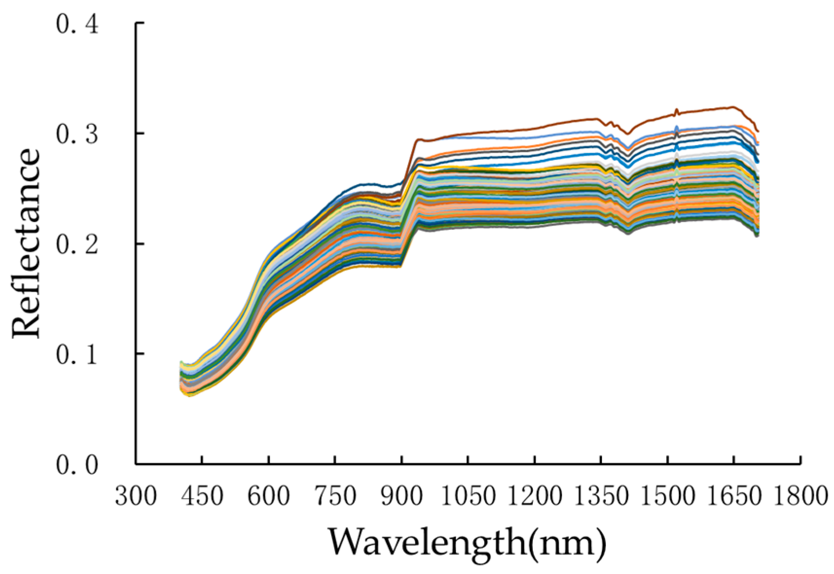
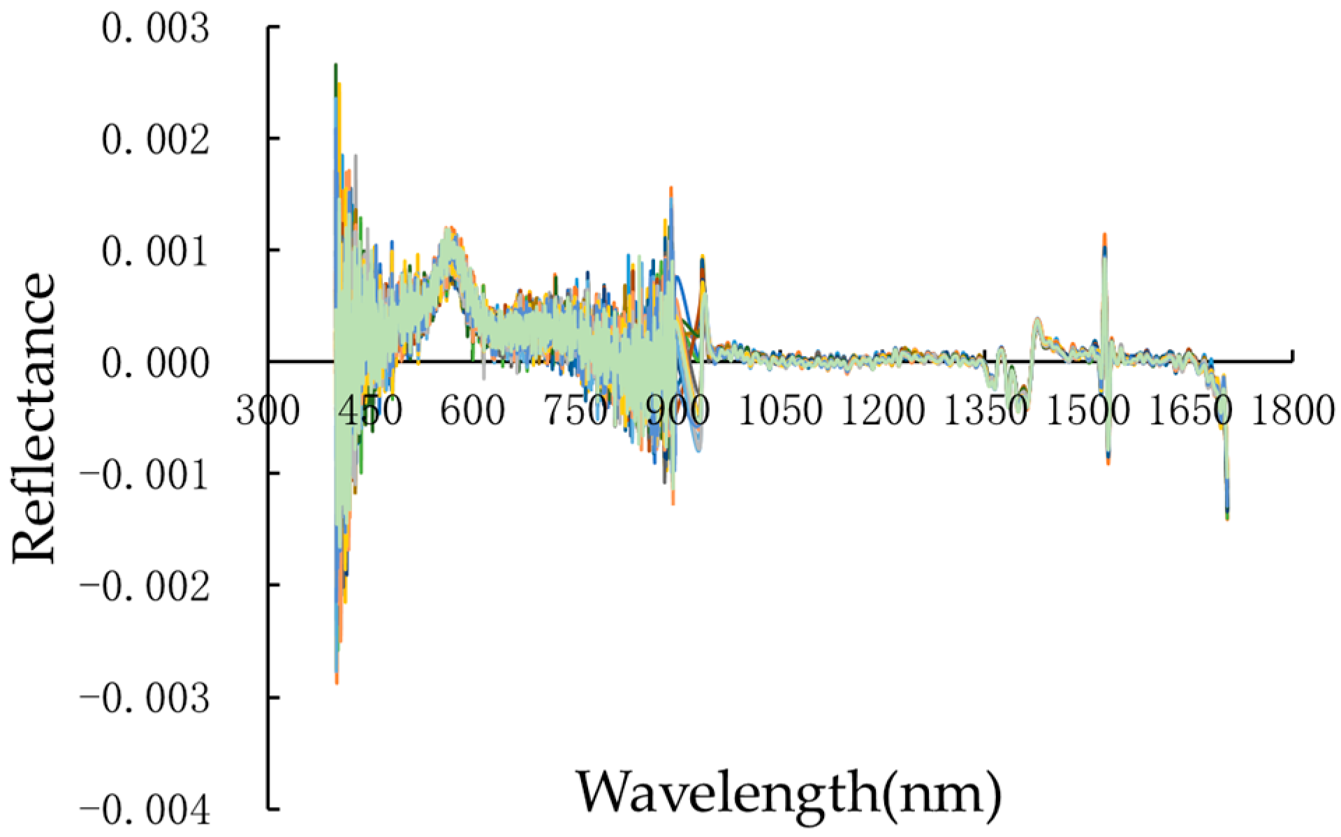
2.1.2. Hyperspectral Data Measurement and Preprocessing

The spectral data acquisition of soil samples was performed with a hyperspectral imager manufactured by Headwall Photonics, Fitchburg, MA, USA. The object distance of the platform was set to 20 nm; the moving speed was 15.55 nm/s; the exposure time was 0.9 ms; the spectral range was 379~1705 nm, and the spectral resolutions of the visible and near-infrared were 0.727 nm and 4.715 nm, respectively. The scanned hyperspectral images were based on the ENVI5.3 platform, and the desired soil sample part was cropped by selecting the region of interest; the spectral reflectance values were extracted by quick statistics from the cropped soil sample images, and the arithmetic mean was taken as the sample. The spectral reflectance value of the soil was extracted from the cropped soil sample image by fast statistics, and the arithmetic mean value was taken as the spectral curve of the sample, which was used as the basic data set for subsequent data processing. Due to the interference of instrumental noise, spectral scattering, and spectral covariance, the accuracy of predicting soil property content using raw spectral data is often low; in order to reduce the error caused by instrumental measurements, the spectral data between 390~1704 nm were selected; at the same time, in order to minimize the influence of noise, S-G smoothing was carried out. It has been shown that the spectral data of the S-G smoothing were effective, which could effectively remove high-frequency noise and interference signals and improve the quality of the data [12,13,14,16,22], and the denoising results are shown in Figure 1. As can be seen from Figure 1, the trends of spectral reflectance of soils with different contents of organic matter were similar. The size of the spectral reflectance of soil organic matter content increases with wavelength, but the growth rate of spectral reflectance decreases. In order to effectively eliminate or attenuate the effect of soil background and to highlight the subtle variations in the spectral curves over different organic matter contents, the S-G smoothing spectral curves were first-order differentiated, and the results of the first-order differential processing are shown in Figure 2. The difference features of the spectral curves after the first-order differential transform are more prominent and can be effectively used for subsequent spectral feature extraction. In order to solve the problem of many hyperspectral bands, large data volume, and redundancy, the arithmetic is reduced to enhance the generalization ability of the model. By adding the L1 paradigm as a penalty term to the loss function, the weight vectors in the model are sparsified, and the weights are compressed to 0, which helps to identify the features that contribute less to the model and, thus, removes redundant or irrelevant features. LASSO regression, by adjusting the strength of the L1 paradigm of the weight vectors, achieves a balance between complexity and overfitting [27,28]. For this reason, this experiment incorporates LASSO regression using L1-paradigm regularization for feature selection.

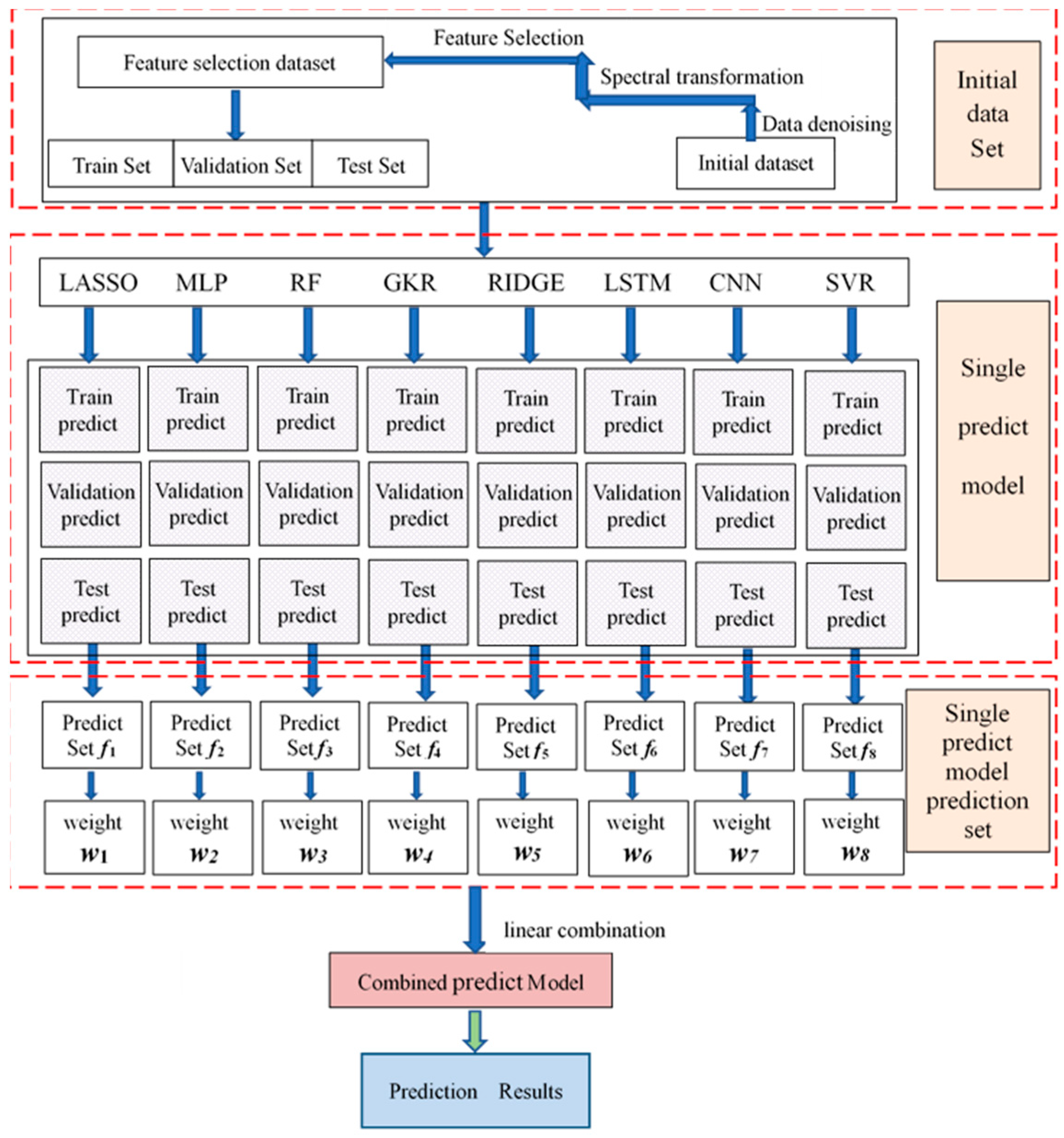
2.2. Construction of the Model

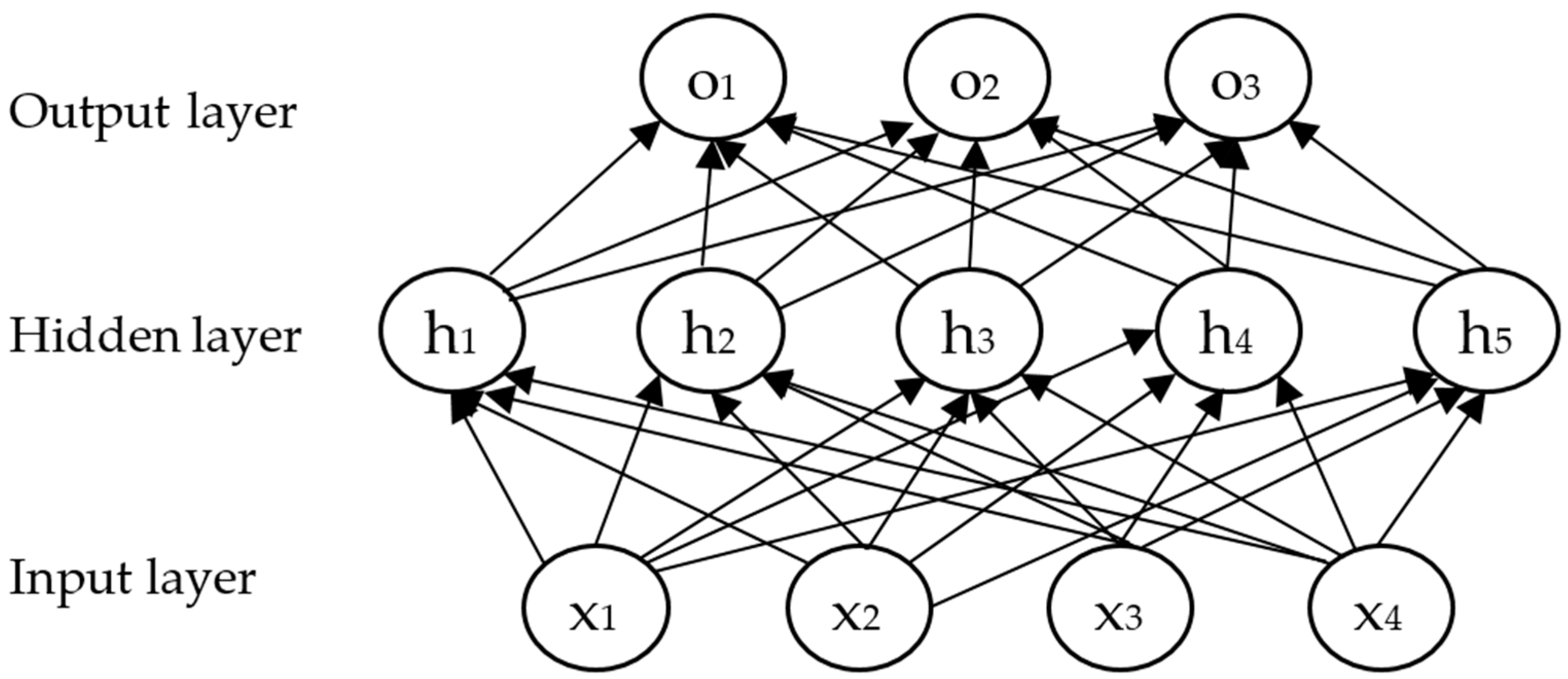
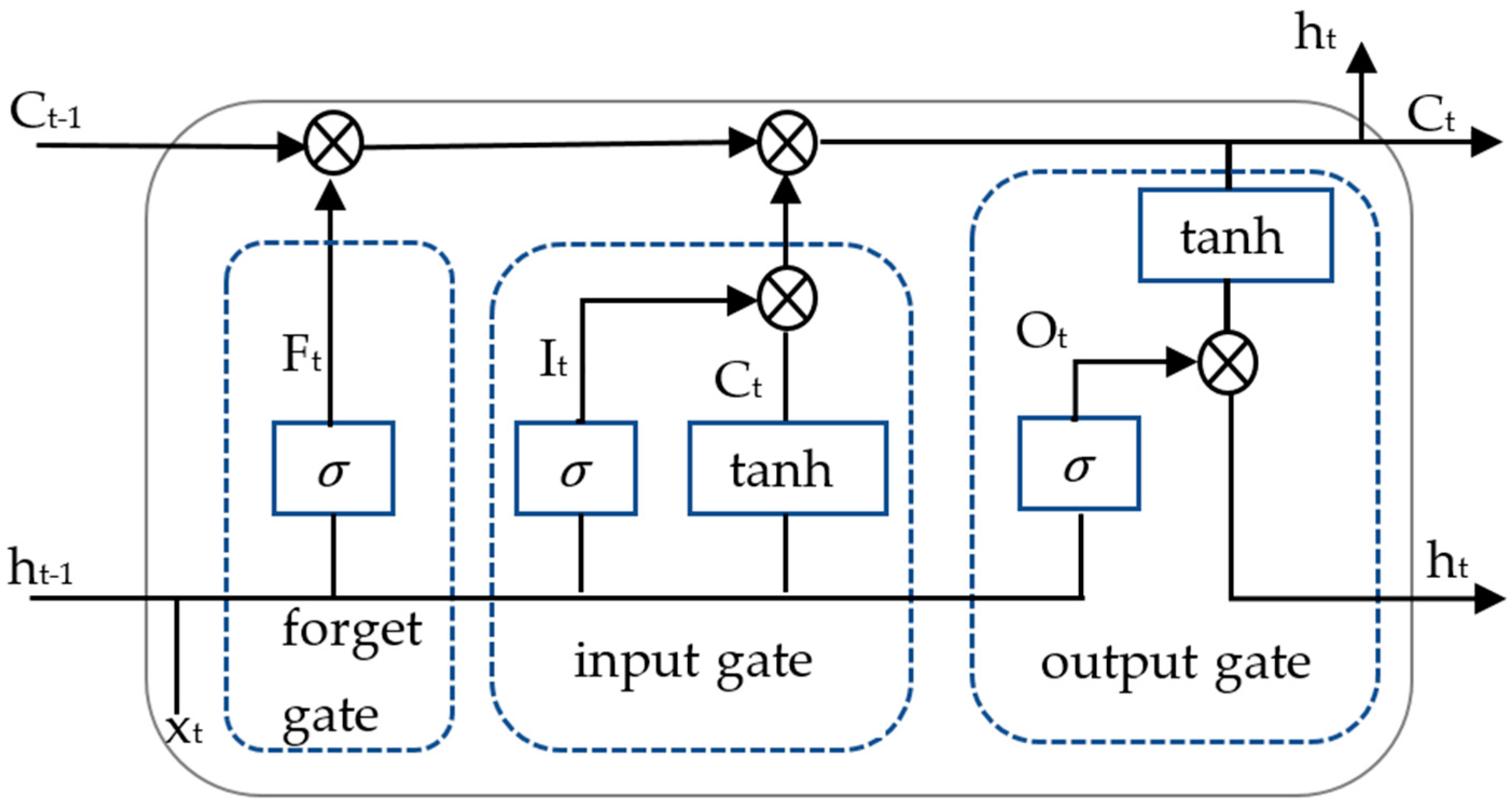
2.2.1. Single-Prediction Model Construction

The spectral dataset was divided into three parts, training set, validation set, and test set, in the ratio of 7:2:1, with 70 spectral data selected by features as the independent variable and soil organic matter content as the dependent variable, using 8 algorithms, such as LASSO Regression (LASSO) (Model 1), Multilayer Perceptron (MLP) (Model 2), Random Forest (RF) (Model 3), Gaussian Kernel Regression (GKR) (Model 4), Ridge Regression (Model 5), Long Short-Term Memory (LSTM) (Model 6), Convolutional Neural Networks (CNN) (Model 7), Support Vector Regression (SVR) (Model 8), to construct a single-prediction model for soil organic matter content, and a superiority of the 8 single-prediction models was proposed.

The LASSO regression [29] is a linear regression using the L1 regularization method that fits the data by minimizing the sum of squares of the residuals with a penalty term, where the penalty term is the L1 norm of the weight vector. By adjusting the strength of the penalty term, LASSO regression can find a balance between complexity and overfitting. In its mathematical formulation, it consists of a linear model with a ${\mathcal{l}}_1$ priori regular terms. Its minimized objective function is $\begin{array}{c}\mathrm{m}\mathrm{i}\mathrm{n}\\ w\end{array}\frac{1}{{2n}_{samples}}{‖X_w-y‖}_2^2+\alpha {‖w‖}_1$, where $\alpha$ is a constant, and ${‖w‖}_1$ is the norm of the parameter vector.

Multilayer Perceptron (MLP) [30] is a feed-forward neural network, including at least three layers of nodes: input layer; hidden layer; and output layer. Its basic structure is shown in Figure 3. In addition to the input nodes, each node is a neuron with nonlinear activation. The regression training process consists of two steps: forward propagation; and backpropagation. The input data for forward propagation are fed to the input layer, which is then passed on to the hidden layer and ultimately generates the output of the output layer. During the backpropagation training process, the outputs are compared to the desired outputs, and an error value is generated. This error is then backpropagated into the network, and the weights are updated accordingly. The MLP uses the mean squared error (MSE) as a loss function and train the model by minimizing this loss function. In the training process, in addition to adjusting the weights and bias terms, regularization techniques can be used to prevent overfitting and improve the generalization ability of the model.

Random Forest (RF) [31] regression is an algorithm based on integrated learning, which performs the regression task by constructing multiple decision trees and integrating their predictions. In Random Forest, each decision tree is independent and trained on a randomly selected subsample, which effectively reduces the risk of overfitting. Random Forests obtain the final regression result by averaging or weighted averaging the predictions of multiple decision trees.

Gaussian Kernel Regression (GKR) [32] is a nonlinear regression model based on the kernel function. It maps the input space to a high-dimensional feature space by introducing a Gaussian kernel function, thus realizing linear regression in a high-dimensional feature space. The Gaussian kernel function is a commonly used kernel function in the form of $\mathrm{K}\left(x,y\right)=\exp \left(-\frac{{‖x-y‖}^2}{{\mathsf{\sigma }}^2}\right)$, where $x$ and $y$ are the samples in the input space, and σ is the width parameter of the Gaussian kernel function, which determines the degree of smoothing of the function.

Ridge Regression [33] is based on the least squares estimation and constrains the size of the coefficient vectors by adding the L2 regularization term, thus solving the instability and inaccuracy of the least squares method on covariate data. The loss function of Ridge regression is as follows: Loss = $\mathrm{L}\mathrm{o}\mathrm{s}\mathrm{s}(y,\mathrm{f}(x;w\left)\right)$ + $\alpha \times \left(\sum {\beta }_i^2\right)$, where $y$ is the actual labeled value; $\mathrm{f}(x;w)$ is the predicted value of the model; w is the parameter of the model; β_i is the ith element of the coefficient vector β, and α is the regularization strength parameter (also known as the ridge parameter or the penalty parameter); by adjusting the value of α, a model complexity by adjusting the value of α, a trade-off can be made between model complexity and prediction accuracy.

Long Short-Term Memory (LSTM) [34] introduces input gate, forget gate, and forget gate on the basis of Recurrent Neural Network (RNN). These gates can selectively control the flow of information, aiming to solve the problem of gradient vanishing and gradient explosion in traditional RNNs while being able to better capture long-term dependencies. Its general structure is shown in Figure 4. The input gate determines how much new information is added to the cell; the forget gate controls whether the information is forgotten at each moment, and the output gate determines whether the information is output at each moment, which is calculated by the following formula (Equation (1)):

$$\begin{array}{c}{F}_t=\sigma \left(w_f\left[h_{t-1},x_t\right]+b_f\right)\\ I_t=\sigma (w_i\left[h_{t-1},x_t\right]+b_i)\\ \widetilde{C_t}=tanh(w_c\left[h_{t-1},x_t\right]+b_c)\\ C_t=F_t\times C_{t-1}+I_t\times \widetilde{C_t}\\ O_t=\sigma (w_o\left[h_{t-1},x_t\right]+b_o\\ h_t=O_t\times tanh\left(C_t\right)\end{array}$$

(1)

In Figure 4 and Equation (1), $w$ and $b$ denote the weights and bias vectors of the above gates, respectively; $C_t$ denotes the memory cell; $\sigma$ and $tanh$ denote the sigmoid activation function and hyperbolic tangent activation function, respectively. $F_t$ is called a forget gate, indicating which features of $C_{t-1}$ are used to calculate $C_t$. $F_t$ is a vector located within the range of [0, 1], typically using sigmoid as the activation function. ⊗ represents the unit multiplication relationship between $F_t$ and $C_{t-1}$. $\widetilde{C_t}$ represents the updated value of the unit state, which is obtained from the input data $x_t$ and hidden node $h_{t-1}$ through a neural network layer, The activation function for the updated value of the unit state is usually $tanh$. $I_t$ is called an input gate, which is a vector between [0, 1] intervals, calculated by $x_t$ and $h_{t-1}$ through the activation function sigmoid. $I_t$ is used to control which features of $\widetilde{C_t}$ are used to update $C_t$. $h_t$ is obtained from the output gate $O_t$ and the unit state $C_t$.

Convolutional Neural Networks (CNN) [34] are mainly based on convolutional operation and backpropagation algorithm; each convolutional layer consists of a number of convolutional units, and the parameters of each convolutional unit are optimized by the backpropagation algorithm. In the training process, the input data are processed by the convolutional layer and activation function to obtain the output result, and then, the output result is compared with the real value to calculate the error. According to the size of the error, the weights and bias terms of the neurons are adjusted layer by layer by the backpropagation algorithm to reduce the error and gradually improve the prediction accuracy.

The goal of Support Vector Regression (SVR) [35] aims to find a suitable $\epsilon -\mathrm{t}\mathrm{u}\mathrm{b}\mathrm{e}$ so that as many sample points as possible are within this tube, and a very small number of sample points outside the tube are considered outliers. When calculating the loss value, although there is a deviation between the sample points in the tube and the predicted value of the objective function, their loss is considered to be 0, which allows for an error of $\epsilon$ between $f\left(x\right)$ and $y$. When the absolute difference between the two is less than $\epsilon$, the loss is considered to be 0. SVR problem based on the training data pairs is as follows: $f\left(x\right)=w,x+b$, where $w$, x represents the dot product of the two vectors $w$ and x. If the regression function f(x) can estimate all the training sample points within the precision ε, the minimization problem could be transformed into the following optimization problem (Equation (2)):

$$\begin{array}{c}min\frac{1}{2}{w}^2\\ s.t.\left\{\begin{array}{c}y-w·x_i-b\le \epsilon \\ w·x_i+b-y\le \epsilon \end{array}i=1,2,\cdots N\right.\end{array}$$

(2)

2.2.2. Combinatorial Predictive Modeling

The combined prediction model is constructed using a linear combination of single-prediction methods [36,37], which is based on the principle (Equation (3)):

$$f_t=w_1{f}_{1t}+w_2{f}_{2t}+\cdots +w_m{f}_{mt}$$

(3)

where $f_t$ is the predicted value of the combined prediction model; f_it is the predicted value of the tth sample of the ith single-prediction method, a total of 8 (m = 8) single-prediction methods, 312 (t = 312) samples of the data selected for this experiment; $w_1{,w}_2{,\cdots , w}_m$ for the weighting coefficients of the m single-prediction methods, the weighting coefficients are obtained through the planning of the solution to the combination of the model as a superior prediction model and satisfy (Equation (4)):

$${\sum }_{i=1}^m{w}_i=1,w_i\ge 0,i=1,2,\cdots m$$

(4)

The process of constructing the combined prediction model is shown in Figure 5.

2.2.3. Calculation of Accuracy Validation Metrics

The model prediction validity is used for the evaluation of prediction accuracy, and its validity is calculated as follows (Equations (5)–(9)):

$$M_i=E\left(A_i\right)\left(1-\sigma \left(A_i\right)\right)$$

(5)

$$E\left(A_i\right)=\frac{1}{n}\sum _{t=1}^n{A}_{it}$$

(6)

$$\sigma \left(A_i\right)={\left[\frac{1}{n}\sum _{t=1}^n{\left(A_{it}-E\left(A_i\right)\right)}^2\right]}^{\frac{1}{2}},i=1,2,3\cdots ,m$$

(7)

$$A_{it}=\left\{\begin{array}{c}1-\left|e_{it}\right| \mathrm{w}\mathrm{h}\mathrm{e}\mathrm{n}\left|e_{it}\right|\le 1\\ 0 \mathrm{w}\mathrm{h}\mathrm{e}\mathrm{n}\left|e_{it}\right|\ge 1\end{array}\right.$$

(8)

$$e_{it}=(x_t-x_{it})/x_t$$

(9)

where $M_i$ is the predictive validity of the ith prediction method; the larger value indicates that the ith prediction method is more effective; $E\left(A_i\right)$ is the mathematical expectation of the sequence of prediction accuracy of the ith prediction method; the larger the value indicates the higher prediction accuracy; $\sigma \left(A_i\right)$ is the standard deviation of the sequence of prediction accuracy of the ith prediction method; the smaller value indicates that the prediction is more stable; i is the number of single-prediction methods, and this paper has used 8 prediction methods; t is the number of prediction samples, and the number of prediction samples in this paper is 312; $x_t$ is the measured value of t samples; $x_{it}$ is the predicted value of the tth sample of the ith prediction method; $e_{it}$ is the relative error of prediction of the tth sample of the ith prediction method; $A_{it}$ is the prediction accuracy of the ith prediction method in the tth sample. When $A_{it}=0$, it indicates that the prediction of the ith prediction method in the tth sample is invalid prediction. The combination-prediction model solution method and process are as follows (Equations (10)–(14)):

(1)

Calculate the combined predicted value of $\widehat{x_t}$

$$\widehat{x_t}=w_1{x}_{1t}+w_2{x}_{2t}+\cdots +w_m{x}_{mt}$$

(10)

where $w_1$, $w_2$, $\cdots$, $w_m$ are the weighting coefficients of m single-prediction methods and satisfy

$${\sum }_{i=1}^m{w}_i=1,w_i\ge 0,i=1,2,\cdots m$$

(11)

(2)

Calculate the relative error $e_t$ and the prediction accuracy $A_t$ of the combination prediction for the tth sample

$$A_t=1-\left|e_t\right|=1-\left|{(x}_t-\widehat{x_t})/x_t\right|=1-{\sum }_{i=1}^m{w}_i{e}_{it}$$

(12)

(3)

Calculate the combination-prediction validity M

$$M=E\left(A\right)\left(1-\sigma \left(A\right)\right)$$

(13)

where $E\left(A\right)$ is the mathematical expectation of the sequence of prediction accuracy of the combination of prediction methods; $\sigma \left(A\right)$ is the standard deviation of the sequence of prediction accuracy of the combination of prediction methods, which is calculated using Equations (5) and (6), and $E\left(A\right)$ and $\sigma \left(A\right)$ are the functions of weighting coefficients $w_1$, $w_2$, $\cdots$, $w_m$ of the various single-prediction methods, so that M is also a function of $w_1$, $w_2$, $\cdots$, $w_m$, denoted as M($w_1$, $w_2$, $\cdots$, $w_m$), denoted as M($w_1$, $w_2$, $\cdots$, $w_m$), and the larger value of M indicates that the combination-prediction method is more effective. The combination-prediction model is calculated and obtained as follows:

$$\begin{array}{l}\hspace{1em}\hspace{1em}\hspace{1em}\hspace{1em}\hspace{1em}\hspace{1em}\hspace{1em}\hspace{1em}\hspace{1em}\hspace{1em}\hspace{1em}\hspace{1em}max M\left(w_1,w_2,\cdots ,w_n\right)\\ \hspace{1em}\hspace{1em}\hspace{1em}\hspace{1em}\hspace{1em}\hspace{1em}\hspace{1em}=\frac{1}{n}{\displaystyle \sum _{t=1}^n}\left[1-\left|{\displaystyle \sum _{i=1}^m}{w}_i{e}_{it}\right|\right]\\ \hspace{1em}\hspace{1em}\hspace{1em}\hspace{1em}\hspace{1em}\hspace{1em}\hspace{1em}·\left\{1-{\left[\frac{1}{n}{\displaystyle \sum _{t=1}^n}{\left(1-\left|{\displaystyle \sum _{i=1}^m}{w}_i{e}_{it}\right|\right)}^2-\frac{1}{n^2}({\displaystyle \sum _{t=1}^n}{(1-\left|{\displaystyle \sum _{i=1}^m}{w}_i{e}_{it}\right|))}^2\right]}^{\frac{1}{2}}\right\}\\ s.t.\left\{\begin{array}{c}\sum _{i=1}^m{w}_i=1\\ w_{i\ge 0},i=1,2,\cdots ,m\end{array}\right.\end{array}$$

(14)

denoted as $M_{min}$ and $M_{max}$ are the minimum and maximum prediction validity of m prediction methods, respectively, and M is the prediction validity of the combination model. Then when M < $M_{min}$, the combination-prediction model is an inferior combination prediction; when $M_{min}$ < M < $M_{max}$, the combination-prediction model is a non-inferior combination prediction; when M > $M_{max}$, the combination-prediction model is a superior combination prediction;

(4)

Approximate solution of the combined prediction model. Since the objective function is not derivable, i.e., the model is non-frivolous nonlinear programming, coupled with the fact that the computational complexity of the model is larger when n and m are larger, the non-frivolous nonlinear programming is transformed into frivolous nonlinear programming to solve the problem. The combined prediction model is equivalent to the following model (Equation (15)):

$$\begin{array}{l}\mathit{max} M\left(w_1,w_2,\cdots ,w_m\right)\\ \hspace{1em}\hspace{1em}\hspace{1em}\hspace{1em}\hspace{1em}\hspace{1em}=\left[{\alpha }_0{\displaystyle \sum _{i=1}^m}{w}_{i}E\left(A_i\right)+(1-{\alpha }_0)\right]\\ \hspace{1em}\hspace{1em}\hspace{1em}\hspace{1em}\hspace{1em}\hspace{1em}·\left\{1-{\alpha }_0{\left[{\displaystyle \sum _{i=1}^m}{w}_i^2{\sigma }^2\left(A_i\right)+{\displaystyle \sum _{i\ne j}}{w}_i{\omega }_j{\rho }_{ij}\sigma (A_i)\sigma (A_j)\right]}^{\frac{1}{2}}\right\}\\ \hspace{1em}\hspace{1em}\hspace{1em}\hspace{1em}\hspace{1em}\hspace{1em}\hspace{1em}\hspace{1em}s.t.\left\{\begin{array}{l}{\displaystyle \sum _{i=1}^m}{w}_i=1\\ w_{i\ge 0},i=1,2,\cdots ,m\end{array}\right.\end{array}$$

(15)

where ${\alpha }_0\in \left[\mathrm{0,1}\right]$ is a constant. The degree of inconsistency of the sign of the relative error of each single-prediction method in the same sample t is taken as different ${\alpha }_0$. The more serious the degree of inconsistency of the sign of the relative error is, the smaller the value of ${\alpha }_0$, and if it is completely consistent, then the value of ${\alpha }_0$ is taken as 1. In this paper, the magnitude of ${\alpha }_0$ is determined according to the ratio of the positive number and the negative number of the relative error in each method and takes a value of 0.9; ${\rho }_{ij}$ is the correlation coefficient of the prediction accuracy sequence of the ith single-prediction method and the jth single-prediction method, and when ${\rho }_{ij}$ ∈ (−1,1), the optimal solution of the combination-prediction model corresponding to the combination-prediction method is the superiority combination prediction. The optimal solution of the combination-prediction model is obtained based on the idea of a nonlinear programming solution.

2.2.4. The Planning and Solving Algorithm for the Combinatorial Predictive Modeling

The optimal solution of the composite forecasting model is obtained based on the Nonlinear Generalized Reduced Gradient (GRG) algorithm [38]. The optimization problem can be simplified as follows (Equation (16)):

$$\left.\begin{array}{c}\min F\left(X\right) X\in E^n\\ s.t. H\left(X\right)=0\\ L\le x\le U L,U\in E^n\end{array}\right\}$$

(16)

where $H\left(x\right)={\left[h_1\left(X\right),h_2\left(X\right),\cdots ,h_m\left(X\right)\right]}^T$, $L={\left[l_1,l_2,\cdots ,l_n\right]}^T$, $U={\left[u_1,u_2,\cdots ,u_n\right]}^T$.

In the solution process, first, all components of X are decomposed into two parts, i.e., $X={\left[X_B,X_N\right]}^T$, where $X_B$ is the basis vector of dimension m, and $X_N$ is the non-basis vector of dimension n-m; correspondingly, $L={\left[L_B, L_N\right]}^T$; $U={\left[U_B, U_N\right]}^T$.

According to the implicit function theorem, it is known that there exists a continuous mapping $X_B=V\left(X_N\right)$; hence, the objective function $F\left(X\right)$ is transformed into $\left(X\right)=F\left(X_B, X_N\right)=f\left(X_N\right)$, making the original objective function $F\left(X\right)$ of n variables into a function $f\left(X_N\right)$ of n-m variables. Therefore, the gradient of $f\left(X_N\right)$ at $X^k$ with respect to $X_N$ is the reduced gradient; then, the reduced gradient of $f\left(X_N\right)$ with respect to $X_N$ is $\nabla f\left(X_N^k\right)={\nabla }_{N}F\left(X^k\right)-{\nabla }_{N}H\left(X^k\right){\left[{\nabla }_{B}H\left(X^k\right)\right]}^{-1}-{\nabla }_{B}F\left(X^2\right)$.

The reduced gradient is denoted briefly as $\nabla f\left(X_N^k\right)={\left[r_1,r_2,\cdots ,r_{n-m}\right]}^T$; define ${\mathrm{S}}^k={\left[s_1,s_2,\cdots ,s_{n-m}\right]}^T$; when $x_{m+j}^k=l_{m+j}$ and $r_j>0$ or when $x_{m+j}^k=u_{m+j}$ and $r_j<0$, then $s_j^k=0$; in other cases, $s_j^k=-r_j$. Make $X_N^{k+1}=X_N^k+{\mathsf{\alpha }\mathrm{S}}^k$, then let $Y_0=X_B^k$ and iterate using the following formula: $Y^{c+1}=Y^c-{\left[{\nabla }_{B}H\left(Y_0{X}_N^{k+1}\right)\right]}^{-1}H(Y^c,X_N^{k+1})$, where $c=1,2,\cdots$, finally obtaining $Y^{c+1}$ that satisfies $H\left(Y^{c+1},X_N^{k+1}\right)=0$ to obtain the optimized value.

3. Results

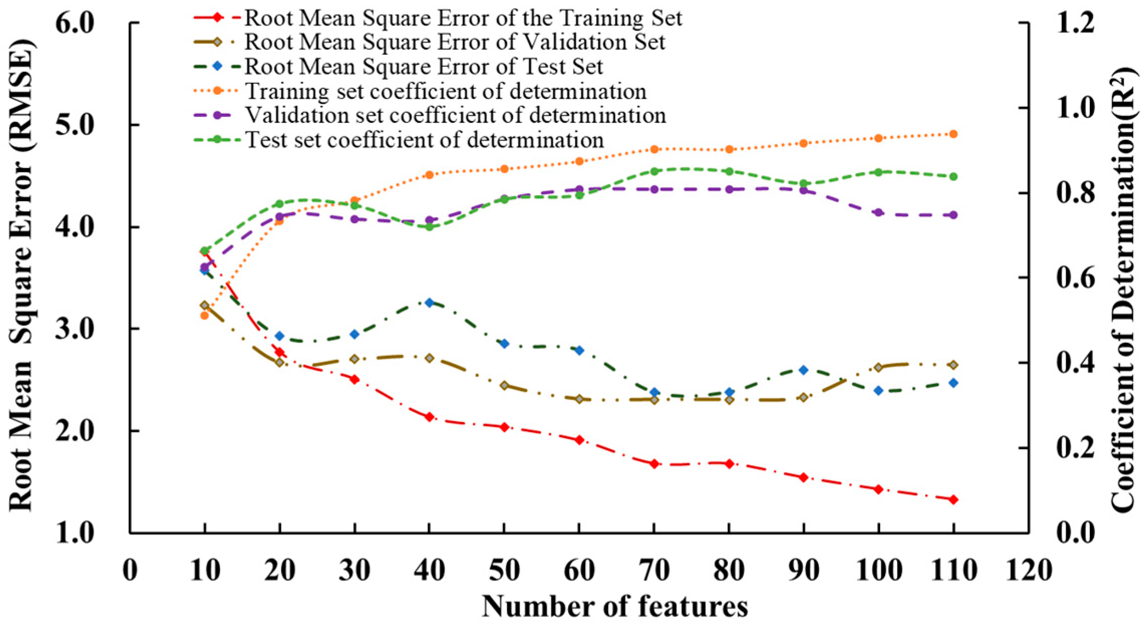
3.1. L1-Paradigm Hyperspectral Feature Selection

Feature selection is carried out by the L1 paradigm; the number of feature selection is set from 10 to 110 in steps of 10 with 11 gradients, and the coefficient of determination R² and the root mean square error RMSE of the training, validation, and test sets are used as the accuracy validations to analyze the optimal number of feature selection, and the results are shown in Figure 6. With the increase in the number of features, the coefficient of determination R² of the training set, validation set, and test set shows an overall increasing trend, and the root mean square error RMSE shows a decreasing trend, but after the number of features reaches 70, the upward trend of the coefficient of determination R² slows down, and the coefficient of determination of the validation set and the test set shows a decreasing trend, and the root mean square error shows a decreasing trend instead of an obvious increase after the number of features is 70, and the model’s performance is not as high as the number of features in the training set, showing the generalization ability of the model. Among the 70 bands selected, the sensitive bands are mainly located at 400–600 nm, 700–900 nm, 1000–1100 nm, and 1400–1600 nm, which is in general agreement with the results of many studies [3,5,16].

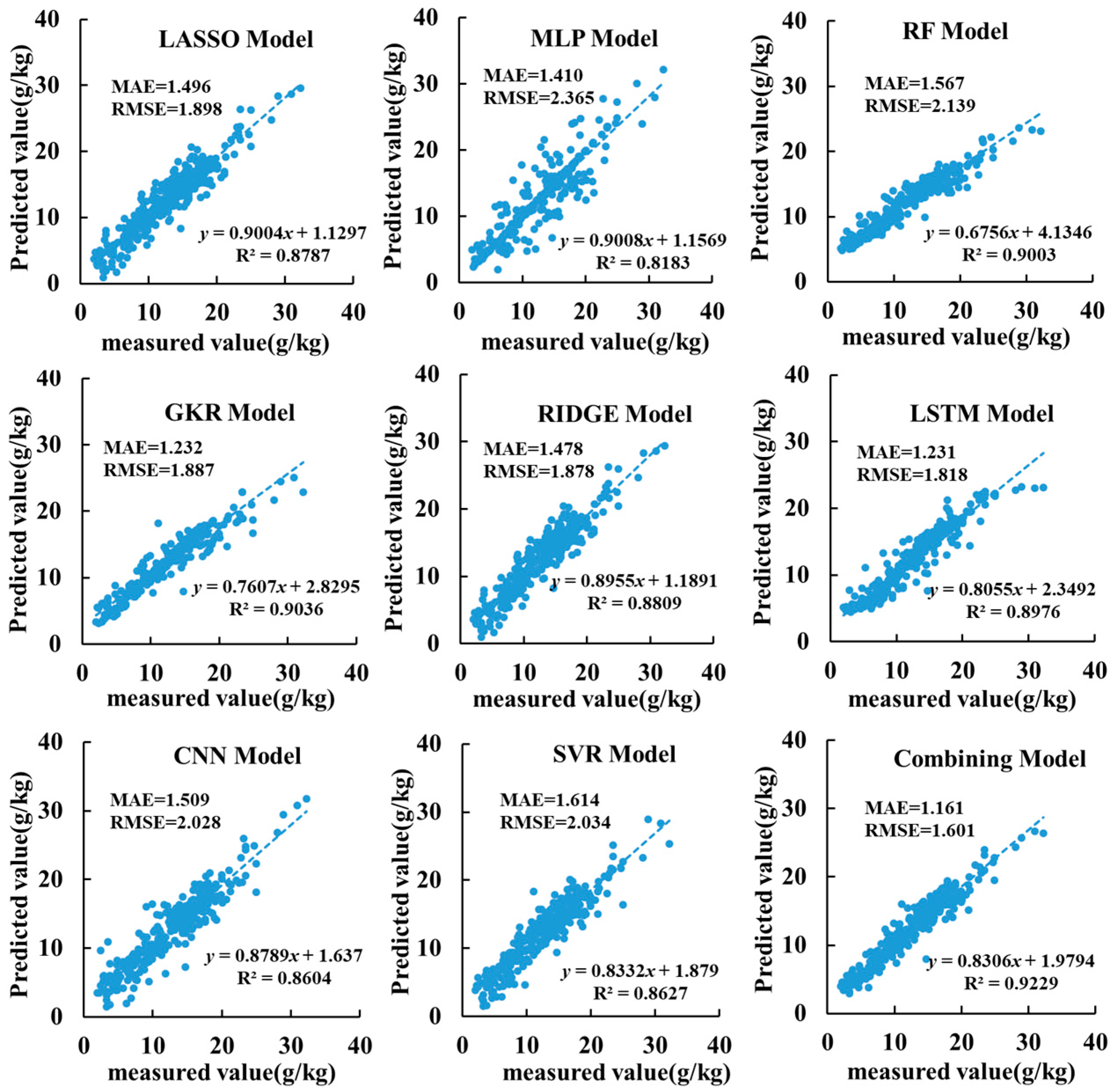
3.2. Results of Single-Prediction Model

Numerous studies have shown that the LASSO, Ridge, MLP, RF, LSTM, CNN, and SVR models used in this study have good prediction results in terms of soil nutrient content, but different spectral pre-processing, different selection of characteristic bands, and different settings of each model parameter in different soil types can affect the prediction accuracy of the model for soil nutrient content [12,17,39]. For example, Zhong Liang et al. [40] explored the prediction accuracy of SOM content of LeNet-5, MLP-5, RF, SVR, and CNN models under different pre-processing, and the results showed that CNN showed a good prediction effect, and SVR was poorer than the other models. Wang Haifeng et al. [41] investigated the organic matter content of desert soil based on the grayscale correlation–ridge regression, and the results showed the ridge regression model could realize a better inversion effect by using only 4% of the full-spectrum band after the transformation of standard normal variables. Deng Yun et al. [22] compared and analyzed the modeling effects of LSTM, PLSR, SVR, and time-convolution networks in different spectral pre-processing of the organic matter content of red soil. Adding self-attention layers to the residual structure of time-convolutional networks can improve learning ability.

The eight selected single-prediction models were used to predict the organic matter content, and the prediction accuracy results are shown in

Table 2. Prediction accuracy of single-prediction models.

Model	Train Set			Validation Set			Test Set			DataSet
	E	σ	M	E	σ	M	E	σ	M	E	σ	M
LASSO	0.865	0.155	0.731	0.836	0.153	0.708	0.802	0.220	0.626	0.853	0.163	0.714
MLP	0.908	0.179	0.746	0.777	0.201	0.621	0.773	0.163	0.647	0.869	0.192	0.702
RF	0.865	0.201	0.691	0.774	0.230	0.595	0.715	0.305	0.497	0.832	0.225	0.645
GKR	0.914	0.134	0.791	0.827	0.159	0.695	0.780	0.244	0.590	0.883	0.161	0.741
Ridge	0.865	0.155	0.731	0.839	0.152	0.712	0.805	0.218	0.630	0.854	0.163	0.715
LSTM	0.901	0.166	0.751	0.814	0.137	0.703	0.785	0.288	0.559	0.872	0.182	0.713
CNN	0.881	0.158	0.742	0.756	0.211	0.597	0.768	0.275	0.556	0.845	0.192	0.683
SVR	0.847	0.162	0.710	0.839	0.130	0.730	0.817	0.229	0.630	0.843	0.164	0.704

. As can be seen from Table 2, considering the three evaluation indexes in the training set E(A4) > E(A2) > E(A3) and σ(A4) < σ(A2) < σ(A3), GKR prediction method is the best, and the RF prediction method is the worst; in the validation set E(A5) > E(A1) > E(A4) > E(A2) > E(A3) and σ(A5) < σ(A1) < σ(A4) < σ(A2) < σ(A3), the ridge prediction method is optimal, and the RF method is the worst; in the test set E(A8) > E(A4) > E(A7) > E(A3) and σ(A8) < σ(A4) < σ(A7) < σ(A3), SVR prediction method is optimal, and the RF prediction method is the worst; in the all dataset E(A4) > E(A5) > E(A8) > E(A3) and σ(A4) < σ(A5) < σ(A8) < σ(A3), GKR prediction method is the best, and RF prediction method is the worst. It can be seen that each model exhibits different prediction accuracies in different datasets.

3.3. Combined Prediction Model

Based on the prediction results of eight single-prediction models, the mathematical expectation $E_i$, standard deviation ${\sigma }_i,$ and correlation coefficient ${\rho }_{ij}$ of the prediction accuracy series of each single-prediction model are calculated. Based on the principle of the combined prediction model and the solution process, the obtained mathematical expectation $E_i$, standard deviation ${\sigma }_i$, and correlation coefficient ${\rho }_{ij}$ are substituted into the optimization model to obtain the maximum prediction validity of the combined model. The objective function $max M\left(w_1,w_2,\cdots ,w_8\right)$ model is solved using the nonlinear Generalized Reduced Gradient (GRG) programming, and the results are as follows: $w_1^{*}=0.099$; $w_2^{*}=0.202$; $w_3^{*}=0.000$; $w_4^{*}=0.357$; $w_5^{*}=0.088$; $w_6^{*}=0.089$; $w_7^{*}=0.000$; $w_8^{*}=0.165$; $M\left(w_1^{\mathrm{*}},w_2^{\mathrm{*}},\cdots ,w_8^{\mathrm{*}}\right)$ = 0.784. The combined model is $f_t=0.099f_{1t}+0.202f_{2t}+0.357f_{4t}+0.088f_{5t}+0.089f_{6t}+0.165f_{8t}$.

The prediction results of the combined prediction model are shown in

Table 3. Prediction accuracy of combination-prediction model.

Evaluating Indicator	LASSO	MLP	RF	GKR	Ridge	LSTM	CNN	SVR	Combining Model
E	0.853	0.869	0.832	0.883	0.854	0.872	0.845	0.843	0.893
σ	0.163	0.192	0.225	0.161	0.163	0.182	0.192	0.164	0.129
M	0.714	0.702	0.645	0.741	0.715	0.713	0.683	0.704	0.778

. From Table 3, it can be seen that the mathematical expectation for the prediction accuracy of the combination model is 0.893, which is greater than the maximum prediction accuracy of a single model. The prediction standard deviation of the combination model is 0.129, which is smaller than the minimum value of the single model prediction standard deviation. The predictive validity of the combination model is 0.778, which is greater than the maximum predictive validity of a single model. Therefore, this combination model is an optimization model, which improves the prediction accuracy compared to a single-prediction model.

Further analysis was conducted on the fitting degree between the true and predicted soil organic matter content values of the eight established single and combination models, and the fitting degree was evaluated through Mean Absolute Error (MAE), Root Mean Square Error (RMSE), and Coefficient of determination (R²) (Figure 7). From Figure 7, it can be seen that the MAEs of the eight models are 1.496, 1.410, 1.567, 1.232, 1.478, 1.231, 1.509, and 1.614, respectively. The MAE of the combined prediction model is 1.161, which is smaller than the minimum MAE in a single model and a 19.487% decrease compared to the average MAE of the eight single models. The RMSE of the eight models are 1.898, 2.365, 2.139, 1.887, 1.878, 1.818, 2.028, and 2.034, respectively. The RMSE of the combined prediction model is 1.601, which is smaller than the minimum RMSE in a single model and a decrease of 20.189% compared to the average MAE of the eight single models. The R² values of the eight models were 0.879, 0.818, 0.900, 0.904, 0.881, 0.898, 0.860, and 0.863, respectively. The R² value of the combined prediction model reached 0.923, which was better than the maximum R² value in a single model and an increase of 5.486% in the average determination coefficient R² compared to the eight single models. The combination model has improved prediction accuracy compared to single models, which is consistent with the results of existing combination models [24].

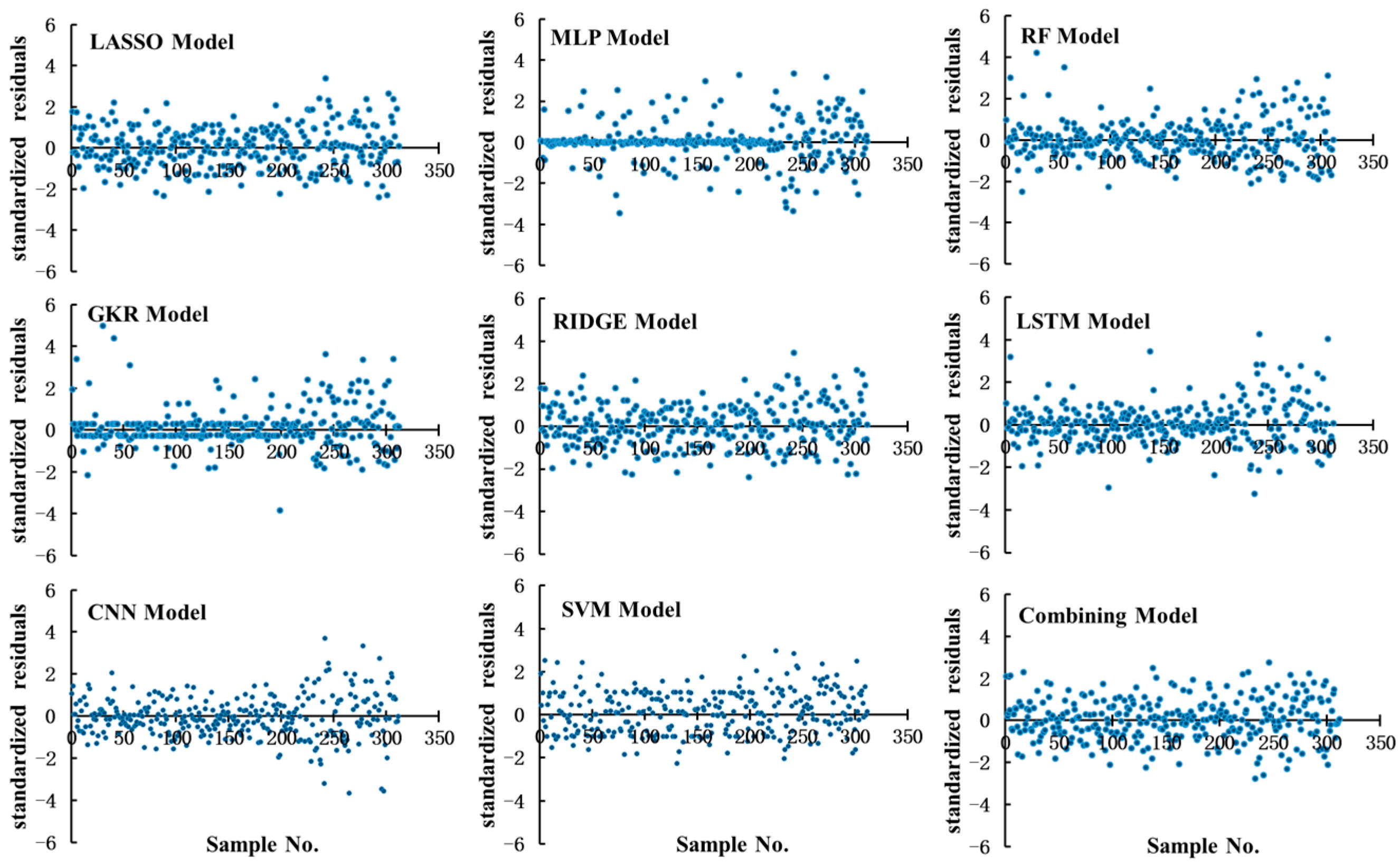
3.4. Residual Analysis

Randomness and unpredictability are key components of any regression model, and residual analysis is a statistical technique used to evaluate whether the regression model accurately predicts observed data. In regression analysis, the relationship between the independent and dependent variables is modeled, and the model is used to predict the value of the dependent variable [16]. Residual is the difference between observed values and model predictions, which can be used to evaluate the fit and prediction accuracy of the model. This study tested the rationality of the model and the reliability of the data through residual plots (Figure 8). From Figure 8, it can be seen that the residuals of the eight single-prediction models and combination-prediction models are all randomly distributed without heteroscedasticity features and do not contain trend information. Both single and combination models are reasonable prediction models, and the residuals of the combination-prediction model are less than eight single-prediction models; 94.23% of the standardized residuals fall between −2 and 2, and the standardized residuals follow a normal distribution.

4. Discussion

In this study, nine methods, L1-paradigm feature selection, L2-paradigm feature selection, tree model feature selection, Kendall feature selection, Pearson feature selection, PCA downscaling, SPE downscaling, t-SNE downscaling, and MDE feature selection, were firstly selected for prediction modeling based on the same dataset, and among the nine feature selection algorithms, L1-paradigm feature selection had the highest prediction accuracy, the main reason being that L1-paradigm minimization made the coefficients of some features become 0, automatically selecting the most important features and eliminating irrelevant or redundant features, and adopting efficient solution methods, such as coordinate descent method and minimum angle regression, etc. What is more, L1-paradigm regularization can efficiently prevent overfitting and improve the model’s generalization ability. For this reason, in this study based on the L1-paradigm feature selection method to select the appropriate number of features according to the trend of the model determination coefficient and the root mean square error with the number of features, a total of 70 sensitive bands were selected, accounting for 8.43% of the total number of bands. This greatly reduces the band information and solves the problem of a large number of bands and large computation in organic matter content prediction.

From the results of the prediction accuracy of single-prediction models (Table 2), it can be seen that for the same set of data sets, the prediction accuracy of different prediction methods on the prediction set, validation set, and training set shows inconsistent phenomena, and the phenomena of underfitting and overfitting may occur; for this reason, it is necessary to take advantage of the advantages of the individual single-prediction models, and innovatively construct the combination model of single models. In the single-prediction models for hyperspectral prediction of organic matter content, the evaluation of prediction accuracy is mostly based on the coefficient of determination, mean absolute error, root mean square error, and other indexes [15,16,17,18,19,20,21,22,23,24,25,26,27,28], and such evaluation indexes mainly take into account the size of the error of each sample, and for the combined prediction model, the sum of the squares of the error or the sum of the absolute value of the error is mostly used as the objective function, with less consideration of the distribution of the error. In this study, the error of prediction accuracy is considered along with the influence of the standard deviation of prediction accuracy on the effectiveness of prediction methods, and the corresponding combined prediction model of prediction effectiveness is established. When the average prediction accuracy of the ith single-prediction method in each sample is greater than the kth, and the standard deviation of the accuracy series of the ith single-prediction method is less than the kth, then the ith single-prediction method can be said to be better than the kth single-prediction method. Therefore, the prediction validity obtained by combining the error and standard deviation is used to evaluate the prediction accuracy of the model through the size of the validity; i.e., when the prediction validity of the ith single-prediction method is greater than the kth, the ith prediction method is said to be better than the kth prediction method. When the predictive validity of the combined prediction model is greater (less) than the predictive validity of each single-prediction model, this combined prediction model is a superior (inferior) combined model; when the predictive validity of the combined prediction model is between the predictive validity of each single-prediction model, this combined prediction model is a non-inferior combined model, and if it is an inferior (non-inferior) combined model, it fails to improve the prediction accuracy. Therefore, in the single-prediction model through the linear combination to build a combination of prediction models, only when the optimal solution of the combination of prediction models will be “better than” the single-prediction method of the “best” in the existing research for the combination of prediction models. The weight coefficients of each single-prediction model in the combination-prediction model are mostly determined by the principle of simple averaging method and inverse error method [24], which may cause the combination-prediction model not to reach the optimal solution; therefore, in this study, we take the maximum predictive validity of the combination-prediction model as the objective function, and the weight coefficients of the single-prediction model are non-negative, and the sum of the weights is 1 as the constraints to carry out the optimal objective planning to solve the optimality of the combination-prediction model, and then we can obtain the optimal combination-prediction model. The superiority of the combination-prediction model is obtained.

The prediction accuracy analysis results of this study show the prediction accuracy of eight single model prediction accuracy prediction validity M from low to high in order of GKR, Ridge, LASSO, LSTM, SVR, MLP, CNN, RF different prediction indexes; the same prediction model performance of the prediction accuracy is not consistent. In the optimal combination model obtained by goal programming solution $w_1^{*}=0.099$, $w_2^{*}=0.202$, $w_3^{*}=0.000$, $w_4^{*}=0.357$, $w_5^{*}=0.088$, $w_6^{*}=0.089$, $w_7^{*}=0.000$, $w_8^{*}=0.165$, $M\left(w_1^{*},w_2^{*},\cdots ,w_8^{*}\right)$ = 0.784 for the superiority model; the combination coefficients calculated by arithmetic averaging are $w_1^{*}=0.127$, $w_2^{*}=0.125$, $w_3^{*}=0.115$, $w_4^{*}=0.132$, $w_5^{*}=0.127$, $w_6^{*}=0.127$, $w_7^{*}=0.122$, $w_8^{*}=0.125$, $M\left(w_1^{*},w_2^{*},\cdots ,w_8^{*}\right)$ = 0.741; the combined prediction model validity of 0.741 is not significantly greater than the maximum value of the single-prediction model prediction validity of 0.741; the prediction accuracy E of 0.882 is less than the maximum value of the prediction accuracy of 0.883 in the single model, for the non-inferiority model; the combination of prediction model constructed by the inverse method of the error in $w_1^{*}=0.123$, $w_2^{*}=0.097$, $w_3^{*}=0.044$, $w_4^{*}=0.206$, $w_5^{*}=0.127$, $w_6^{*}=0.129$, $w_7^{*}=0.057$, $w_8^{*}=0.217$, $M\left(w_1^{*},w_2^{*},\cdots ,w_8^{*}\right)$ = 0.751, and the combined prediction model validity 0.751 is greater than the maximum value of the prediction validity of single-prediction model, but the prediction accuracy E is 0.881 less than the maximum value of the prediction accuracy in the single model 0.883, which is a non-inferior model; the weight coefficients of RF and CNN single-prediction models in the superior model are 0, which indicates that these two single-prediction models are redundant prediction methods compared to the combined prediction model obtained by the inverse error method, which is a good choice for improving the accuracy and generalization ability of the combined prediction model and also simplifying the complexity of the model. And the combined prediction model is at least a non-inferior prediction when the correlation coefficient ${\rho }_{ij}\in \left(-\mathrm{1,1}\right)$ of the prediction accuracy series of any two single-prediction models, the combined prediction method is superior combined prediction method, and the condition of correlation coefficient ${\rho }_{ij}\in \left(-\mathrm{1,1}\right)$ is easy to satisfy in general so that the combined prediction model makes use of information provided by the individual prediction models to a greater extent. This study is only a preliminary analysis of the combined prediction model in the prediction of organic matter content with respect to the prediction effectiveness indexes, and all the sample data selected in the construction of the combined prediction model are obtained by calculation, and the number of single-prediction models selected is also limited; the processing of the spectral data is also only first-order differentiation, and the feature extraction is only the L1-paradigm feature algorithm, and different fractional orders can be introduced in the next step. The next step could be to introduce different fractional-order differential processing techniques and multiple feature extraction and to select more single-prediction models for benchmarking in order to establish a more comprehensive and appropriate combined prediction model to improve the accuracy and generalization of prediction. A more comprehensive and appropriate combined prediction model is needed in the future to improve the accuracy of SOM prediction.

5. Conclusions

Compared with the single model, the combined forecasting model adopted in this paper can integrate the forecasting results of multiple single models, and make the final forecasting results more accurate through certain weight distribution. Because different models may be affected by different factors, the combined forecasting model can make full use of the advantages of each model to reduce the deviation of the prediction results of a single model.

Compared with the single model, the combination forecasting model adopted in this paper can reduce the risk of the single model by integrating multiple models, making the final forecasting results more stable and reliable.

The combination-prediction model based on prediction effectiveness used in this article is at least a non-inferiority combination model, which can determine whether a single-prediction model used in constructing a composite model is redundant, achieving higher prediction accuracy and model stability with fewer single models.

References

1. Liao, Y.; Wen, L.; Kong, X.; Zhang, L.; Cheng, J.; Sun, X. Spatio-temporal Variability and Influencing Factors of Soil Organic Matter in Cultivated Land of Daxing District in Recent 40 Years. Chin. J. Soil Sci. 2020, 51, 40–49. [Google Scholar]
2. Tao, Z.; Xu, Z.; Ding, J.; Zhang, Y. Determination of soil organic matter content under forest based on different methods. Sci. Technol. Eng. 2022, 22, 3892–3901. [Google Scholar]
3. Prathibha, S.R.; Hongal, A.; Jyothi, M.P. IOT Based Monitoring System in Smart Agriculture. In Proceedings of the 2017 International Conference on Recent Advances in Electronics and Communication Technology (ICRAECT), Bangalore, India, 16–17 March 2017; IEEE: Piscataway, NJ, USA, 2017. [Google Scholar]
4. Zhao, M.; Xie, Y.; Lu, L.; Li, D.; Wang, S. Modeling for Soil Organic Matter Content Based on Hyperspectral Feature Indices. Acta Pedol. Sin. 2021, 58, 42–54. [Google Scholar]
5. Guo, J.; Long, H.; He, J.; Mei, X.; Yang, G. Predicting soil organic matter contents in cultivated land using Google Earth Engine and machine learning. Trans. Chin. Soc. Agric. Eng. (Trans. CSAE) 2022, 38, 130–137. [Google Scholar]
6. Ou, D.; Tan, K.; Lai, J.; Jia, X.; Wang, X.; Chen, Y.; Li, J. Semi-supervised DNN regression on airborne hyperspectral imagery for improved spatial soil properties prediction. Geoderma 2021, 1, 114875. [Google Scholar] [CrossRef]
7. Jiao, C.; Zhen, G.; Xie, X.; Cui, X.; Shang, G. Prediction of Soil Organic Matter Using Visible-Short Near-Infrared Imaging Spectroscopy. Spectrosc. Spectr. Anal. 2020, 40, 3277–3281. [Google Scholar]
8. Tian, Y.; Zhang, J.; Yao, X.; Cao, W.; Zhu, Y. Laboratory assessment of three quantitative methods for estimating the organic matter content of soils in China based on visible/near-infrared reflectance spectra. Geoderma 2013, 202, 161–170. [Google Scholar] [CrossRef]
9. Zhang, T.; Yu, L.; Yi, J.; Nie, Y.; Zhou, Y. Determination of Soil Organic Matter Content Based on Hyperspectral Wavelet Energy Features. Spectrosc. Spectr. Anal. 2019, 39, 3217–3222. [Google Scholar]
10. Meng, X.; Bao, Y.; Ye, Q.; Liu, H.; Zhang, X.; Tang, H.; Zhang, X. Soil Organic Matter Prediction Model with Satellite Hyperspectral Image Based on Optimized Denoising Method. Remote Sens. 2021, 13, 2273. [Google Scholar] [CrossRef]
11. Zhang, Z.; Lao, C.; Wang, H.; Arnon, K.; Chen, J.; Li, Y. Estimation of Desert Soil Organic Matter through Hyperspectra Based on Fractional-Order Derivatives and SVMDA-RF. Trans. Chin. Soc. Agric. Mach. 2020, 51, 156–167. [Google Scholar]
12. Shang, T.; Chen, R.; Zhang, J.; Wang, Y. Estimation of soil organic matter content in Yinchuan Plain based on fractional derivative combined with spectral indices. Chin. J. Appl. Ecol. 2023, 34, 717–725. [Google Scholar]
13. Cai, H.; Zhou, L.; Shi, Z.; Ji, W.; Luo, D.; Peng, J.; Feng, C. Hyperspectral Inversion of soil organic matter in Jujube Orchard in Southern Xinjiang Using CARS-BPNN. Spectrosc. Spectr. Anal. 2023, 43, 2568–2573. [Google Scholar]
14. Ran, S.; Ding, J.; Ge, X.; Liu, B.; Zhang, J. Estimation Method of VIS-NIR Spectroscopy for Soil Organic Matter Based on Sparse Networks. Laser Optoelectron. 2020, 57, 381–389. [Google Scholar]
15. Tang, H.; Meng, X.; Su, X.; Ma, T.; Liu, H.; Bao, Y.; Zhang, M.; Zhang, X.; Huo, H. Hyperspectral prediction on soil organic matter of different types using CARS algorithm. Trans. Chin. Soc. Agric. Eng. 2021, 37, 105–113. [Google Scholar]
16. Zhang, X.; Li, Z.; Zheng, D.; Song, H.; Wang, G. VIS-NIR Hyperspectral Prediction of Soil Organic Matter Based on Stacking Generalization Model. Spectrosc. Spectr. Anal. 2023, 43, 909–910. [Google Scholar]
17. Zhou, W.; Xiao, J.; Li, H.; Chen, Q.; Wang, T.; Wang, Q.; Yue, T. Soil organic matter content prediction using Vis-NIRS based on different wavelength optimization algorithms and inversion models. J. Soils Sediments 2023, 23, 2506–2517. [Google Scholar] [CrossRef]
18. Lin, Z.D.; Wang, Y.B.; Wang, R.J.; Wang, L.S.; Lu, C.P.; Zhang, Z.Y.; Song, L.T.; Liu, Y. Improvements of the Vis-NIRS Model in the Prediction of Soil Organic Matter Content Using Spectral Pretreatments, Sample Selection, and Wavelength Optimization. J. Appl. Spectrosc. 2017, 84, 529–534. [Google Scholar] [CrossRef]
19. He, S.; Shen, L.; Xie, H. Hyperspectral Estimation Model of Soil Organic Matter Content Using Generative Adversarial Networks. Spectrosc. Spectr. Anal. 2021, 41, 1905–1911. [Google Scholar]
20. Zhou, H.; Li, X.; Shang, X.; Miao, C.; Huang, C.; Lu, J. Hyperspectral estimation of soil organic matter based on particle swarm optimization neural network. Sci. Surv. Mapp. 2019, 44, 146–150. [Google Scholar]
21. Wu, J.; Guo, D.; Li, G.; Guo, X.; Zhong, L.; Zhu, Q.; Guo, J.; Ye, Y. Prediction of Soil Organic Carbon Content in Jiangxi Province by Vis-NIR Spectroscopy Based on the CARS-BPNN Model. Sci. Agric. Sin. 2022, 55, 3738–3750. [Google Scholar]
22. Deng, Y.; Niu, Z.; Feng, Q.; Wang, Y. Anovel Hyperspectral prediction model of organic matter in red soil based on improved temporal convolutional network. Spectrosc. Spectr. Anal. 2023, 43, 2942–2951. [Google Scholar]
23. Chun, X.; Jing, H.; Yao, X.; Yong, B.; Zhe, Y. Modeling and Prediction of Soil Organic Matter Content Based on Visible-Near-Infrared Spectroscopy. Forests 2021, 12, 1809. [Google Scholar] [CrossRef]
24. Xie, W.; Zhao, X.; Guo, X.; Ye, Y.; Sun, X.; Kuang, L. Spectrum Based Estimation of the Content of Soil Organic Matters in Mountain Red Soil Using RBF Combination Model. Sci. Silvae Sinivae 2018, 54, 16–23. [Google Scholar]
25. Huang, X.; Du, L.; Hong, J.; Wang, S.; Lian, Z.; Zhang, G.; Jiang, L.; Zhang, L.; Ye, L. Correlation between potassium dichromate external heating method and ASI for the determination of soil organic matter. Hubei Agric. Sci. 2020, 15, 122–125. [Google Scholar]
26. Wang, Y.; Li, Z. Effect of potassium dichromate dosage on the determination of soil organic carbon by sulfur-chromium oxidation. Environ. Prot. Circ. Econ. 2011, 31, 57–58+65. [Google Scholar]
27. Liu, L.; Fan, X.; Liao, Z. Dimension Reduction Model via Joint L1-trace Norms and Optimization Algorithm. J. China Railw. Soc. 2013, 35, 69–74. [Google Scholar]
28. Liu, J.; Luan, X.; Liu, F. Near Infrared Spectroscopic Modelling of Sodium Content in Oil Sands Based on Lasso Algorithm. Spectrosc. Spectr. Anal. 2018, 38, 2274–2278. [Google Scholar]
29. Ranstam, J.; Cook, J.A. LASSO regression. J. Br. Surg. 2018, 105, 1348. [Google Scholar] [CrossRef]
30. Sun, Z.; Xue, L.; Xu, Y.; Wang, Z. Overview of deep learning. Appl. Res. Comput. 2012, 29, 2806–2810. [Google Scholar]
31. Liu, J.; Dong, Z.; Xia, J.; Wang, H.; Meng, T.; Zhang, R.; Han, J.; Wang, N.; Xie, J. Estimation of soil organic matter content based on CARS algorithm coupled with random forest. Spectrochim. Acta Part A Mol. Biomol. Spectrosc. 2021, 258, 119823. [Google Scholar] [CrossRef]
32. Huang, F.; Liu, Y.; Chen, B. Prediction model of network traffic based on combined kernel function Gaussian regression. Comput. Eng. Appl. 2015, 51, 93–97. [Google Scholar]
33. Wei, L.; Yuan, Z.; Wang, Z.; Zhao, L.; Zhang, Y.; Lu, X.; Cao, L. Hyperspectral Inversion of Soil Organic Matter Content Based on a Combined Spectral Index Model. Sensors 2020, 20, 2777. [Google Scholar] [CrossRef] [PubMed]
34. Wang, H.; Zhang, L.; Zhao, J.; Hu, X.; Ma, X. Application of Hyperspectral Technology Combined with Genetic Algorithm to Optimize Convolution Long- and Short-Memory Hybrid Neural Network Model in Soil Moisture and Organic Matter. Appl. Sci. 2022, 12, 10333. [Google Scholar] [CrossRef]
35. Rui, J.; Zhang, H.; Zhang, D.; Han, F.; Guo, Q. Total organic carbon content prediction based on support-vector-regression machine with particle swarm optimization. J. Pet. Sci. Eng. 2019, 180, 699–706. [Google Scholar] [CrossRef]
36. Chen, H.; Hou, D. Combination forecasting model based on forecasting effective measure with standard deviate. J. Syst. Eng. 2003, 18, 203–210. [Google Scholar]
37. Wang, Y.; Liao, Z.; Mathieu, S.; Bin, F.; Tu, X. Prediction and evaluation of plasma arc reforming of naphthalene using a hybrid machine learning model. J. Hazard. Mater. 2021, 404 Pt A, 123965. [Google Scholar] [CrossRef]
38. Ma, W.; Wang, H.; Rui, Q. Research on Model Updating for Tracked Vehicle Dynamic Model Based on Generalized Reduced Gradient Method. J. Syst. Simul. 2012, 24, 774–779. [Google Scholar]
39. Ma, Y.; Jiang, Q.; Meng, Z.; Liu, H. Black Soil Organic Matter Content Estimation Using Hybrid Selection Method Based on RF and GABPSO. Spectrosc. Spectr. Anal. 2018, 38, 181–187. [Google Scholar]
40. Zhong, L.; Guo, X.; Guo, J.; Xu, Z.; Zhu, Q.; Ding, M. Hyperspectral estimation of organic matter in red soil using different convolutional neural network models. Trans. Chin. Soc. Agric. Eng. (Trans. CSAE) 2021, 37, 203–212. [Google Scholar]
41. Wang, H.; Zhang, Z.; Arnon, K.; Chen, J.; Han, W. Hyperspectral estimation of desert soil organic matter content based on gray correlation-ridge regression model. Trans. Chin. Soc. Agric. Eng. 2018, 34, 124–131. [Google Scholar]
Figure 1. Spectral curve of S−G denoising.
Agronomy 14 00789 g001
Figure 2. Spectral curve of first−order differential transformation.
Agronomy 14 00789 g002
Figure 3. MLP structure.
Agronomy 14 00789 g003
Figure 4. LSTM neural network structure.
Agronomy 14 00789 g004
Figure 5. Combined prediction model construction process.
Agronomy 14 00789 g005
Figure 6. Accuracy verification of the number of different feature bands.
Agronomy 14 00789 g006
Figure 7. The degree of fit and error analysis between the predicted and measured values of each model.
Agronomy 14 00789 g007
Figure 8. Residual analysis results of the model.
Agronomy 14 00789 g008