Abstract
Accurate positioning at the inter-row canopy can provide data support for precision variable-rate spraying. Therefore, there is an urgent need to design a reliable positioning method for the inter-row canopy of closed orchards (planted forests). In the study, the Extended Kalman Filter (EKF) fusion positioning method (method C) was first constructed by calibrating the IMU and encoder with errors. Meanwhile, 3D Light Detection and Ranging (LiDAR) observations were introduced to be fused into Method C. An EKF fusion positioning method (method D) based on 3D LiDAR corrected detection was designed. The method starts or closes method C by the presence or absence of the canopy. The vertically installed 3D LiDAR detected the canopy body center, providing the vehicle with inter-row vertical distance and heading. They were obtained through the distance between the center of the body and fixed row spacing. This can provide an accurate initial position for method C and correct the positioning trajectory. Finally, the positioning and canopy length measurement experiments were designed using a GPS positioning system. The results show that the method proposed in this study can significantly improve the accuracy of length measurement and positioning at the inter-row canopy, which does not significantly change with the distance traveled. In the orchard experiment, the average positioning deviations of the lateral and vertical distances at the inter-row canopy are 0.1 m and 0.2 m, respectively, with an average heading deviation of 6.75°, and the average relative error of canopy length measurement was 4.35%. The method can provide a simple and reliable inter-row positioning method for current remote-controlled and manned agricultural machinery when working in standardized 3D crops. This can modify the above-mentioned machinery to improve its automation level.
1. Introduction
Orchards and planted forests are widely distributed worldwide [1]. Recently, precision variable-rate spraying has received much study in orchards and planted forests [2,3,4]. It requires precise canopy characteristics to provide data [5,6]. The geometric characteristics of plants are directly related to their growth and productivity. They can be used as indicators for estimating plant biomass and growth, yield, water consumption, health assessment, and long-term productivity testing [7,8]. Among them, canopy volume is the most commonly used canopy characteristic [9]. The canopy volume requires sensors to provide length, width and height [10]. The width and height are provided by distance sensors, and accurate canopy length requires highly accurate positioning sensors and methods [11].
At present, there are three main positioning methods: absolute, relative and fusion positioning [12]. The absolute positioning method actively or passively senses the surrounding information through its sensors, thereby achieving absolute positioning based on the external environment [13]. This is mainly the Global Navigation Satellite System (GNSS) positioning method. Because of its high positioning accuracy, it has been widely used in agriculture [14]. Many studies have shown that the positioning accuracy of GNSS in field crops is more than 95% [15]. However, it is susceptible to weather and cannot be used in rainy, snowy or foggy weather [13]. Due to tree occlusion, the GNSS signal in orchards and planted forests is weak even with no signal [16]. Hence, the mounted position of the GNSS antenna is raised to receive GNSS signals [13]. Nevertheless, its installation is too high, and is highly susceptible to vibration and terrain changes. This will greatly affect the positioning accuracy of GNSS. The relative positioning method mainly uses sensors such as the Inertial Measurement Unit (IMU) and encoder [12]. It requires an accurate initial position and motion estimation method, and the obtained position is relative. It does not need to perceive the external environment, but only its own motion state [17]. Therefore, it is not easily affected by the weather and the surroundings. It has been widely used in fields. There are inherent errors in each sensor so they cannot be eliminated and accumulate with time [13]. It has high positioning accuracy for a short time, but is not suitable for long time precise positioning [17,18,19].
The fusion positioning method combines the advantages of the absolute positioning method, which has high accuracy in perceiving the surroundings, and the relative positioning method, which does not rely on the external environment. [12,20,21]. Therefore, it has been widely used in recent years [22]. Among them, the most typical method is the Simultaneous Localization and Mapping (SLAM) [23]. The method obtains high positioning accuracy, but the algorithm is complex and requires high computing [24,25]. The sensors of the method to perceive the surroundings are mainly visual sensors and Light Detection and Ranging (LiDAR) [25,26,27]. The LiDAR has the advantages of high positioning accuracy, large data, and less susceptibility to weather [28]. This makes LiDAR widely used in crop detection and navigation [21,29,30]. Among them, horizontally mounted LiDAR is used for navigation and vertically mounted for crop detection [31,32]. The horizontal installation of 3D LiDAR has a narrow vertical field of view so that the entire plant canopy can be measured far away from the canopy [33]. While the vertical installation can obtain abundant plant information on both sides, providing massive data support for variable-rate spraying, the narrow horizontal view cannot be used for navigation.
In summary, absolute positioning methods are highly susceptible to surroundings. Relative positioning methods have high positioning accuracy in a short time and low positioning accuracy in a long time. The fusion positioning methods are complex, with high computing demand, and the LiDAR needs to be installed horizontally. To address the above issues, we use a single vertically installed 3D LiDAR and relative positioning sensors (encoder and IMU) to achieve high-precision positioning and canopy length measurement at the inter-row canopy. Thus, 3D LiDAR is used to detect the presence or absence of the canopy and determine the absolute inter-row positioning (heading and inter-row vertical coordinates) of the vehicle. This can correct the data acquired by the positioning method (method C) based on the Extended Kalman Filter (EKF) at the canopy. The method C and the sensor starts or closes according to the presence or absence of the canopy. When restarting, the inter-row lateral coordinates (0) between rows are acquired. Meanwhile, the advantages of the relative positioning method with high positioning accuracy for a short time are utilized. When the method C is restarted, it can provide high-precision positioning and canopy length measurement at the inter-row canopy. The above is the EKF fusion positioning method (method D) based on 3D LiDAR corrected detection. In this study, we make the following hypotheses:
- (1)
- Mechanical vibration has no effect on sensor accuracy.
- (2)
- There is no significant magnetic field change in the surroundings.
- (3)
- Temperature changes have no effect on the sensor.
It is limited because the method is mainly for modern orchards (planted forests) with fixed row spacing. Yet, it provides new methods and new ideas for the inter-row canopy positioning in modern orchards (planted forests) and can be extended to other 3D crops that are planted in a standardized manner. The method has a wide range of uses in 3D crops grown in fixed row spacing with weak and no GNSS signals. It is simple and reliable, and can be used to modify existing agricultural machinery into intelligent machinery.
2. Materials and Methods
2.1. Composition and Electronic Hardware System of Information Collection Vehicle
The hereby designed information collection vehicle (ICV), with dimensions of 1.2 m × 0.45 m × 1.5 m in length, width and height, respectively, and a maximum load of 200 kg, is shown in Figure 1a. The ICV mainly consists of an electronic hardware system, a chassis walking system, and a positioning system. The electronic hardware system is integrated, which can sense the surroundings in real-time, and obtain information about the ICV (Figure 1b). It is divided into a sensor module, processing module and power module in accordance with the functions. The chassis walking system is the vehicle shown in Figure 1a, which provides support for other systems. Meanwhile, the positioning system is the GPS shown in Figure 1b and can obtain the ICV trajectory.
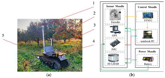
Figure 1.
Composition and electronic hardware system of ICV. (a) ICV, and (b) Electronic hardware system design. 1. 3D LiDAR, 2. GPS, 3. Notebook PC, 4. Battery, 5. Chassis walking system. The green line in (b) indicates the power supply, while the others represent the information transmission.
2.1.1. Chassis Walking System
The chassis walking system is a Bunker chassis produced by AgileX Robotics Co., Ltd. (Shenzhen, China), with dimensions of 1.2 m × 0.4 m × 0.45 m in length, width and height, respectively, powered by 48 V. The active wheels drive the rubber tracks that move the ICV forward, the eight loading wheels support the body weight, and four guiding wheels are used to guide and support the tracks and adjust the tightness of the tracks. The ICV achieves differential steering and 360° in-situ steering by means of different speeds of the left and right active wheels. The spring suspension was designed to give the ICV high ground clearance and good ground adaptation. When walking, the maximum moving speed of ICV is 3.0 m/s, the maximum climbing angle is 30°, and the minimum distance between the frame and the ground is 20 cm, which allows it to move flexibly in the orchard. We added a controller to its interior to realize the function of traveling at a certain speed. In this study, the ICV is implemented at a speed of 1 m/s. Operators only need to control the left and right directions of the ICV and prevent collisions and bumps.
2.1.2. Sensor Module
The sensor module mainly consists of 3D LiDAR, an encoder, an IMU, etc. LiDAR senses the surroundings of the ICV and provides data support for auxiliary positioning. The 16-wire mechanical LiDAR produced by RoboSense Technology Co., Ltd. in Shenzhen, China, can uninterruptedly scan the surrounding trees at 360° horizontally and 30° vertically (15° above and below the LiDAR level), and provide up to 300,000 points per second, with a maximum detection distance of 150 m, a detection accuracy of ±2 cm, and a vertical angle resolution of 2°. The horizontal angle resolution is 0.09°, 0.18° and 0.38° while working at 5 Hz, 10 Hz and 20 Hz, respectively (10 Hz is hereby adopted), with DC 12 V power supply and 100 M Ethernet communication with the notebook PC.
The encoder and IMU acquire the vehicle speed, heading angle and position information. The encoder is an E6B2-CWZ6C encoder (Omron, Osaka, Japan) with a resolution of 1000 P/R (pulse/ring), and is co-axially connected to the active wheel (diameter 22 cm) of the ICV via a connecting shaft. The IMU is a WT61C-RS485 IMU manufactured by Dongguan Weite Intelligent Technology Co., Ltd., Guangzhou, China, with a Kalman filter program, and provides stable and accurate data. The static accuracy is 0.05°/s; the dynamic accuracy is 0.2°/s in X and Y directions; the Z-axis accuracy is 1°/s without magnetic field interference; the acceleration accuracy is 0.0005 g; the gyroscope accuracy is 0.061°/s; and the maximum data output frequency is 200 Hz (100 Hz is hereby adopted).
2.1.3. Processing Module
With a data volume of 300,000 point clouds per second, the central processing unit (CPU) must be extremely powerful. For this reason, we chose a notebook PC equipped with an i7 8750H processor, 16 G of RAM, 128 G of SSD, NVIDIA GeForceGTX1050Ti GPU, 1 T of Mechanical hard drive, Windows 10 pre-installed, RS232, Ethernet, USB, and RS485 communication interfaces. This study requires MCU to take the encoder information and upload it to the notebook PC. In this paper, the M3S type STM32 MCU produced by QiXingChong Company in Dongguan, China is hereby selected, which has a chip of stm32f103zet6, cortex-M3 protocol, 144 pins, 512k flash memory, 72 MHz main frequency, and multiple communication interfaces such as CAN, USB, RS232 and RS485. The GPS module, MCU, and IMU are connected to the notebook PC through USB, RS232, and RS485 communication interfaces, respectively.
2.1.4. Power Module
In addition to the functional modules mentioned above, a power module is required to provide the power supply for each module. In this case, a 12 V ternary lithium battery (6S-12000mAh, Shenzhen, China) with a battery capacity of 12,000 mAh and a full charge voltage of about 22.2 V is selected. A voltage regulation module and a power display module are built-in, which can continuously supply power for 2–4.5 h under normal conditions and make automatic alarms when the voltage is lower than 11.5 V using a buzzer. It takes about 1.5 h to be fully charged. Meanwhile, there are voltage regulators installed to provide stable voltage for different functional modules (5 and 12 V power supply).
2.1.5. Positioning System
To verify the positioning performance of the ICV, the mobile trajectory measurement system needs to have a high accuracy so that it can be directly used as the reference true value. The “QFQ3” RTK GNSS positioning system produced by China Quanfang Navigation Company (Shenzhen, China), which is compatible with GLONASS, Galileo, QZSS, SBAS, BDS, and GPS, is hereby adopted. The positioning system incorporates real-time differential algorithms to provide centimeter positioning accuracy, ±1 cm horizontal positioning accuracy, initialization time < 5 s, data output frequency up to 20 Hz (20 Hz is used), and a power supply range of 5 to 24 V DC. The RTK GNSS mobile station (±2.5 cm movement accuracy) on the robot has a linear distance of 0.5 m from the center of the body and a vertical distance of 0.2 m.
2.2. The Fusion Positioning Method Based on EFK
There are inherent measurement errors in the encoder and IMU due to factors such as manufacturing and installation. The measurement error of the encoder was corrected by STM32 MCU encoder mode, whereas the IMU was corrected by the ellipsoid correction method (Appendix A).
2.2.1. Kinematic Model
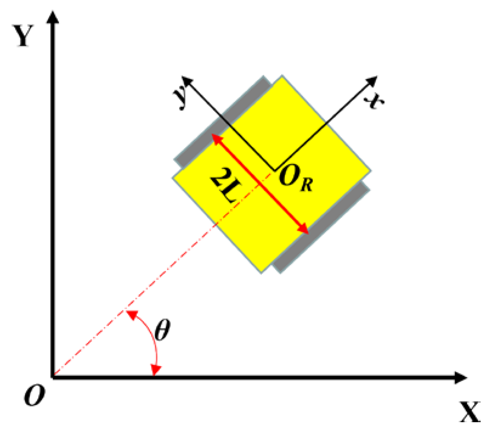
The ICV kinematic model was constructed from kinematic and relative positioning sensor (encoder and IMU) data (Figure 2).

Figure 2.
Kinematic model. Two coordinate systems are included in the figure, one is the world coordinate system and the other is the body coordinate system. The heading angle (), wheelbase (2L), and body center (OR) of the vehicle are also labeled in the figure.
The kinematic model of the relative positioning method is constructed from the initial position and the data provided by the sensors (Equation (1)).
where, is the current motion state of the ICV; is the previous motion state of the ICV; is the change of the motion state of the ICV within the moment; , , , , and are the X-axis displacement, Y-axis displacement, heading angle, X-axis velocity and Y-axis velocity of the ICV at the previous moment, respectively; , , , and are the change of X-axis displacement, Y-axis displacement, heading angle, X-axis velocity and Y-axis velocity of the ICV within the moment, respectively; , and are the current angular velocity, X-axis acceleration and Y-axis acceleration of the ICV, respectively.
Meanwhile, the expression form of and is as follows:
2.2.2. Measurement Model
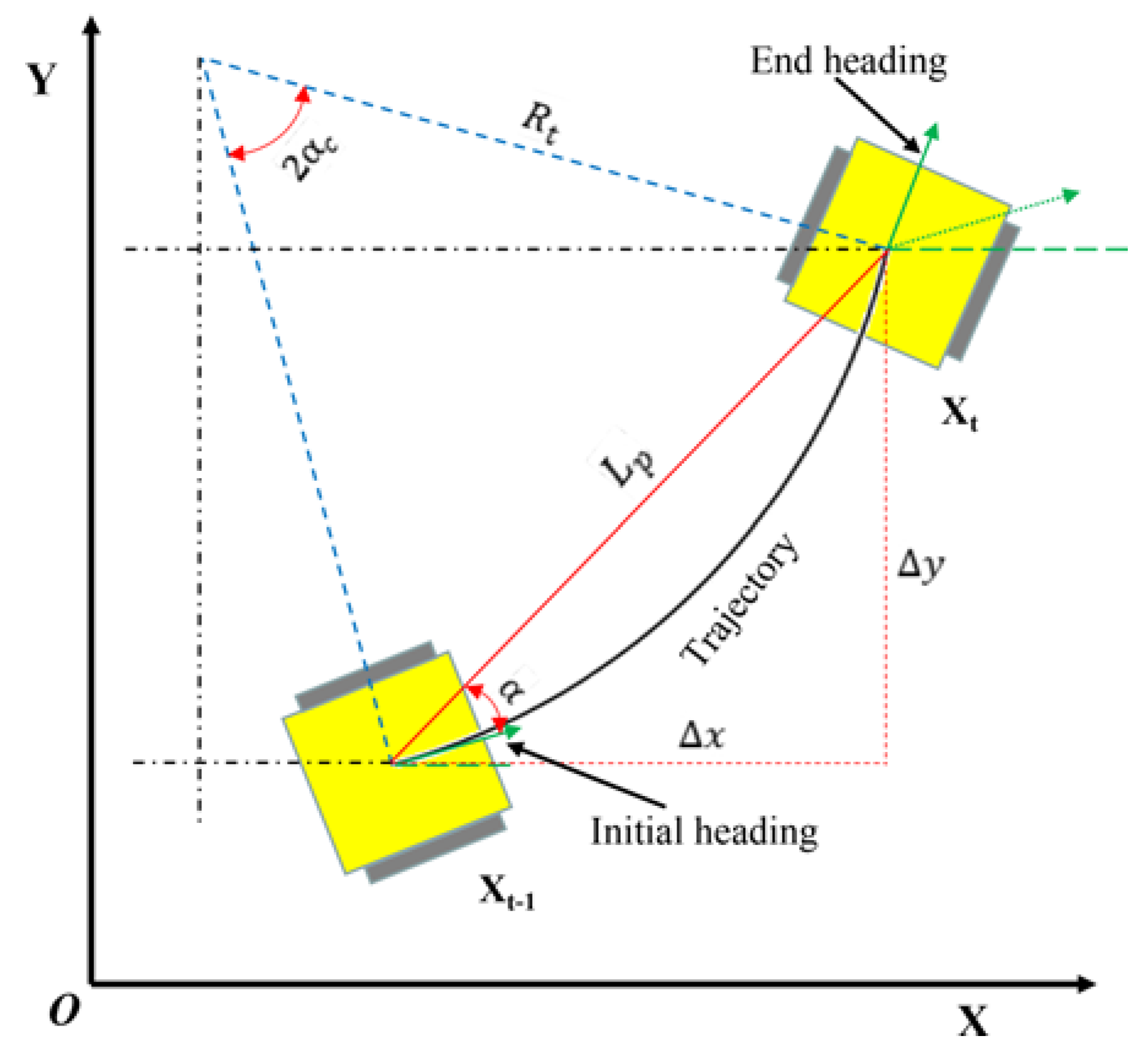
After the ICV kinematic model is determined, its measurement model needs to be constructed. The model should clearly represent the process of and the change of ICV motion through the encoder (Figure 3).
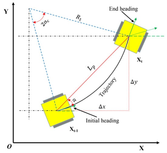
Figure 3.
Encoder measurement model based on the sine theorem. The ICV heading, trajectory, displacement (LP), displacement change ( and ) and heading deviation (2αc) are clearly shown. α is the chord tangent angle, so α = αc, which is half of the heading deviation.
According to the geometric relationship and the sine theorem (Figure 3), the displacement increment of the ICV in the world coordinate can be obtained. Therefore, the increment () of the X-axis in world coordinates is:
where, is the ICV displacement; is the initial heading angle; is the heading deviation; is the encoder pulses number for the left side of the ICV’s active wheel; is the encoder pulse number for the right side of the ICV’s active wheel; is half of the active wheel distance on both sides; and is the pulse in one rotation.
So, the increment () of the Y-axis in world coordinates is:
From this, the position and attitude of the ICV at any moment () is obtained as:
It is incomplete to construct the measurement model only by the encoder, and the measurement model constructed by the IMU is also required. When the ICV is moving, the measurement model of the ICV at the moment obtained by the IMU is:
where, and are the X-axis and Y-axis displacements at the moment , respectively, and obtained by integrating the acceleration twice; is the heading angle; are the X-axis and Y-axis velocities at the moment , respectively, and obtained by integrating the acceleration; are the X-axis and Y-axis angular velocities at the moment , respectively, and obtained by integrating the acceleration, respectively; are the X-axis and Y-axis accelerations at the moment , respectively.
2.2.3. EKF Fusion Positioning Method Based on Encoder and IMU Data
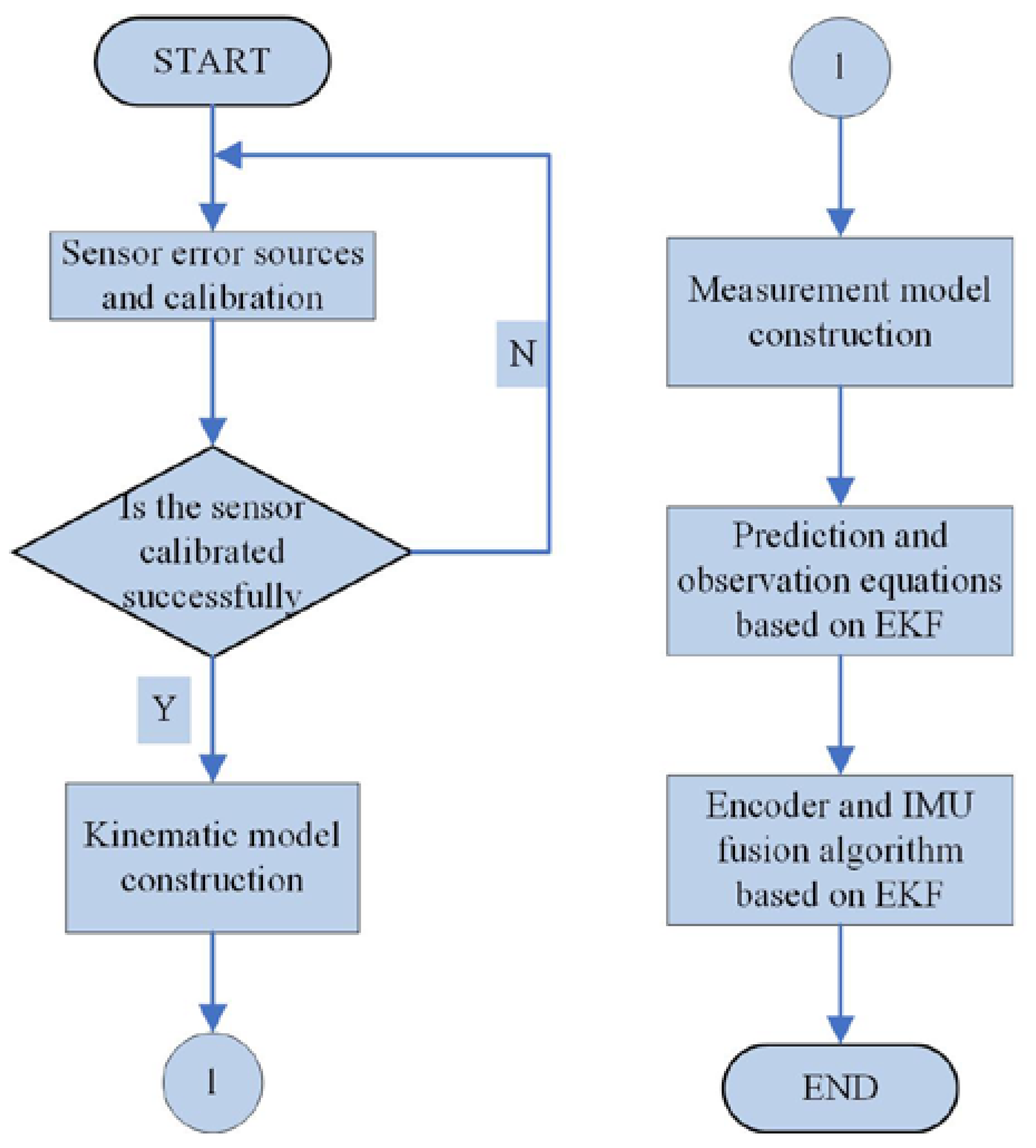
Multi-sensor fusion positioning needs to minimize the effect of sensor noise. The data from the encoder and IMU are fused, which are used to reduce errors and improve positioning accuracy. The encoder has high accuracy in measuring speed and determining displacement, whereas the IMU has high accuracy in angular velocity and acceleration measurement. Therefore, the measured data between the encoder and IMU can be complementary. In this study, the EKF algorithm is used to fuse the two measured data to realize the estimation, prediction and measurement of the real-time position of the ICV (Appendix B) [34]. The flowchart of the method C is shown in Figure 4.
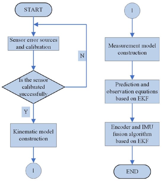
Figure 4.
Flowchart of method C.
2.3. Methods for Obtaining the Vertical Position of the Canopy Body Center
The tree canopy is normally distributed and its body center is a stump. Because the LiDAR in this study is installed vertically, only part of the canopy can be detected. The canopy body centers cannot be obtained in real time through the whole tree point cloud. In this study, a threshold (0.75 times the row spacing) was used to determine whether there was a canopy on both sides of the ICV. If not, the point cloud was removed. If there is, the point cloud within one frame (0.1 s) was sparsely processed to reduce computational difficulty. Then, the point cloud was transformed into a voxel point with a length of 2 cm. And the mean of the point cloud is obtained by Singular Value Decomposition (SVD). At the mean position, the plane was constructed perpendicular to the tree rows. The point cloud on the plane is fitted to a circle by the Least Squares method. The circle center is the canopy body center of the point cloud for that frame. The vertical coordinate of the circle center is the vertical distance of the body center.
2.4. Principle of Accurate Positioning at the Inter-Row Canopy
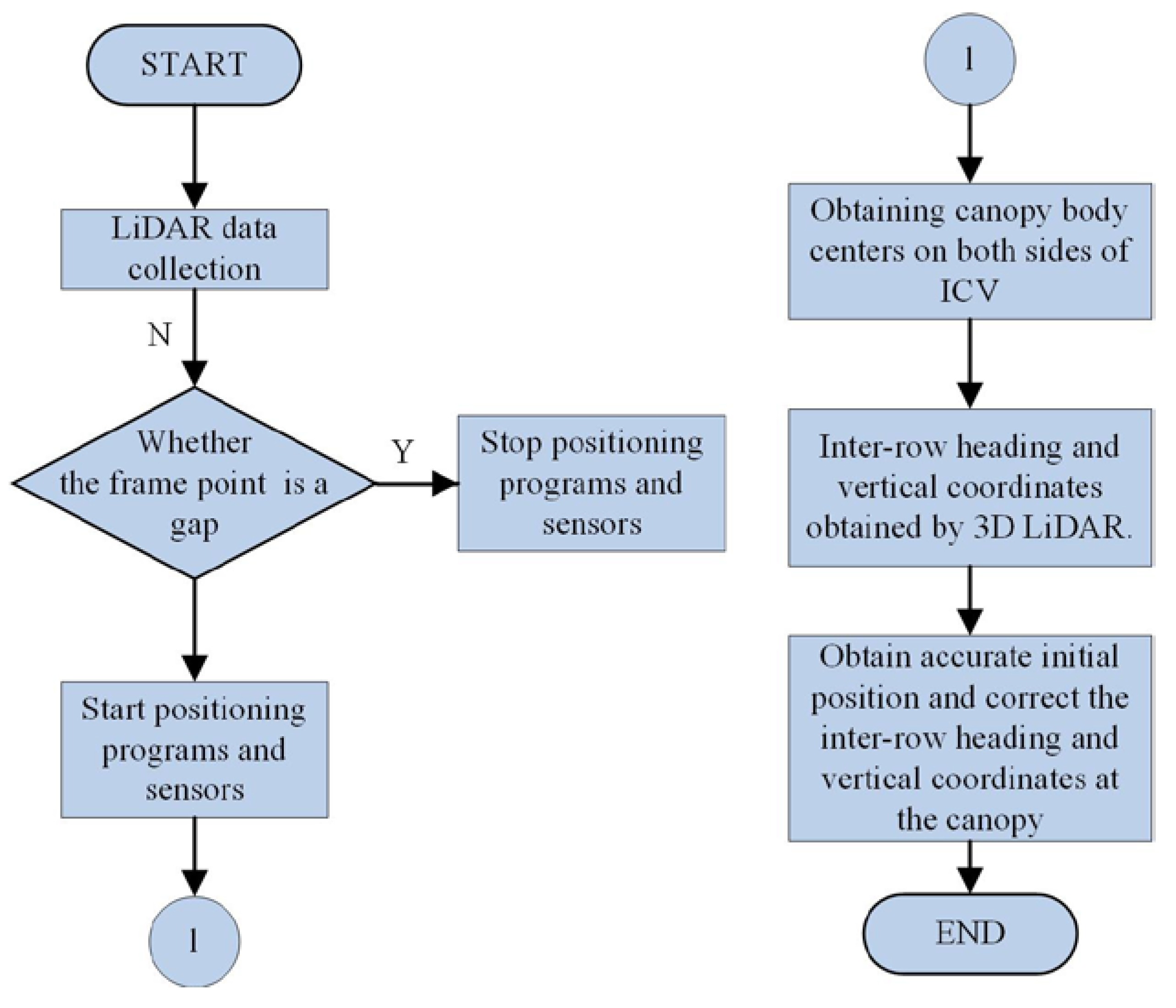
The relative positioning method has high positioning accuracy in a short time. There are gaps between canopies in some orchards and planted forests. According to the above characteristics, method D is designed (Figure 5). After the electronic hardware system is powered on, 3D LiDAR senses the surrounding information and processes it. It first determines whether the point cloud is a gap or not. If there is a gap, the IMU, encoder and the method C will stop. If there is a canopy, start. When restarting, the heading and inter-row vertical coordinates of the initial position are obtained (Figure 6). Additionally, the inter-row lateral coordinates of the initial position are 0. At the inter-row canopy, the heading and vertical coordinates are obtained by 3D LiDAR in real time. It can be corrected for the heading and vertical coordinates of the method C.
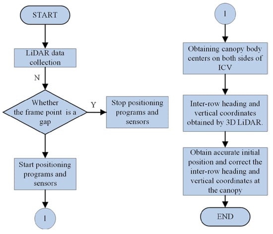
Figure 5.
Flowchart of method D.
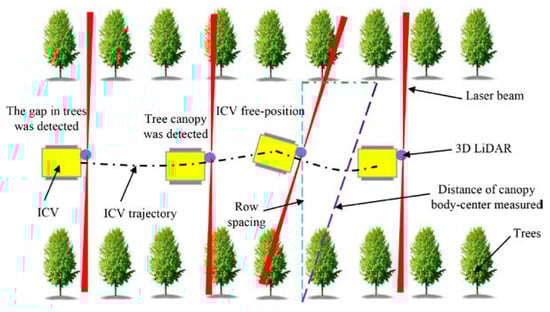
Figure 6.
Principle diagram of method D. The laser beam detects tree canopies or gaps on both sides when the ICV is traveling between rows.
When the ICV is driving in orchards (planted forests) with fixed row spacing, the gaps and canopies on both sides can be detected by 3D LiDAR (Figure 6). When the ICV travels to any position, its heading (Equation (7)) and the vertical coordinates (Equation (8)) at the inter-row canopy can be obtained. They are calculated by the distance of inter-row canopy body-centered vertical coordinates on both sides and the row spacing. The above is the method D designed in this study. As a result, the purpose of high-precision positioning of the ICV can be obtained at the inter-row canopy.
From the geometric relationship in Figure 6, we can get:
where, is the heading angle; is the row spacing; is the vertical distance of the canopy body centers on both sides detected by 3D LiDAR.
Based on the heading angle, row spacing and the vertical distance detected by 3D LiDAR, the inter-row vertical coordinate (Equation (8)) is obtained.
where, is the inter-row vertical coordinate; is the vertical distance detected by LiDAR from the body center to the left canopy; is the vertical installation distance between LiDAR and ICV axis.
2.5. Experimental Design
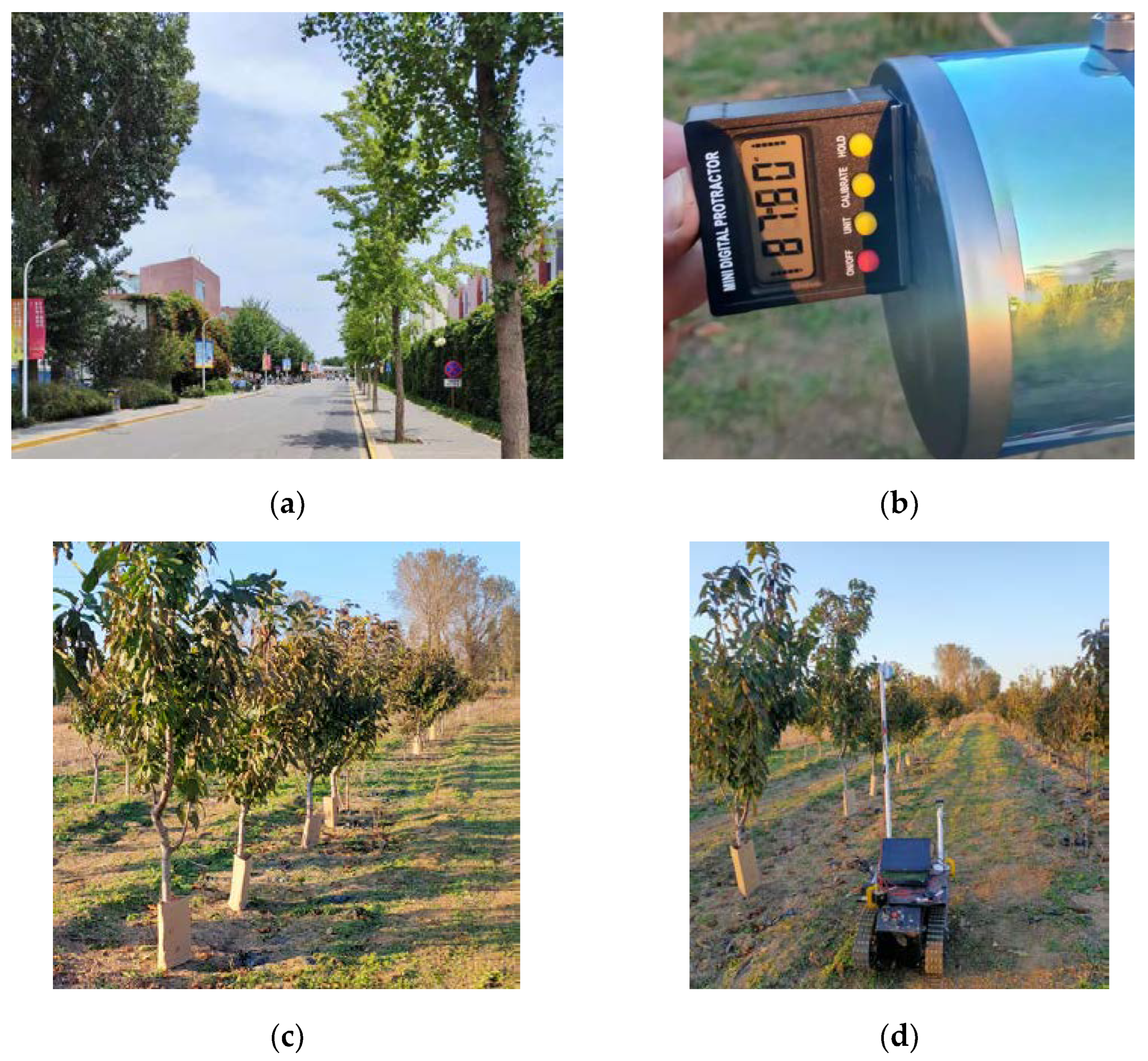
To verify the positioning and canopy length measurement accuracy of method D at the inter-row canopy, campus and orchard comparison experiments were designed. The encoder positioning method (method A), the weighted average fusion positioning method (method B) of the encoder and IMU data (the weighted proportion of encoder is 0.4, and IMU is 0.6), and method C are compared with method D. In this case, the method D uses GPS positioning at the gap to ensure the positioning integrity. On 12 October 2021, ginkgo trees on both sides of the road (Figure 7a) were selected for the experiment on the sidewalk of China Agricultural University (116.2915° E, 40.0357° N) with good GPS signals. The average tree height of the trees is 10.56 m, with a plant spacing of 7.5 m, a row spacing of 15 m, and an average maximum length of 3.58 m. The length of the test area is 40 m, with a total of 8 ginkgo trees on both sides, which are divided into 4 tree groups.
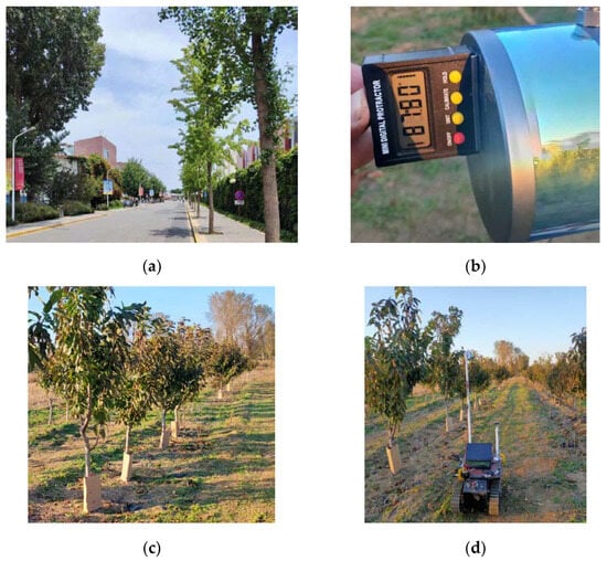
Figure 7.
Situation of the experimental campus and orchard. (a) Ginkgo trees on both sides of the sidewalk; (b) 3D LiDAR installation angle correction; (c) experimental orchard situation; (d) experimental site. The figures include both campus and orchard experimental site conditions. The two topographies are obviously different.
After each experiment, a digital inclinometer (PT180, produced by R&D Instruments, Shenzhen, China, with a measurement range of −90°~90° and an accuracy of 0.01°) is used to correct the 3D LiDAR installation angle (Figure 7b).
2.5.1. Positioning Accuracy
The GPS base station is placed in the middle of the tree row. Moreover, the GPS module is used to determine the latitude and longitude of the stumps and the boundary of the test area. The GPS mobile station is installed on the ICV to record its real-time trajectory. The ICV is controlled to move forward using a remote control. When it reaches the end point, the positioning algorithm program is stopped. The experiment is repeated 5 times.
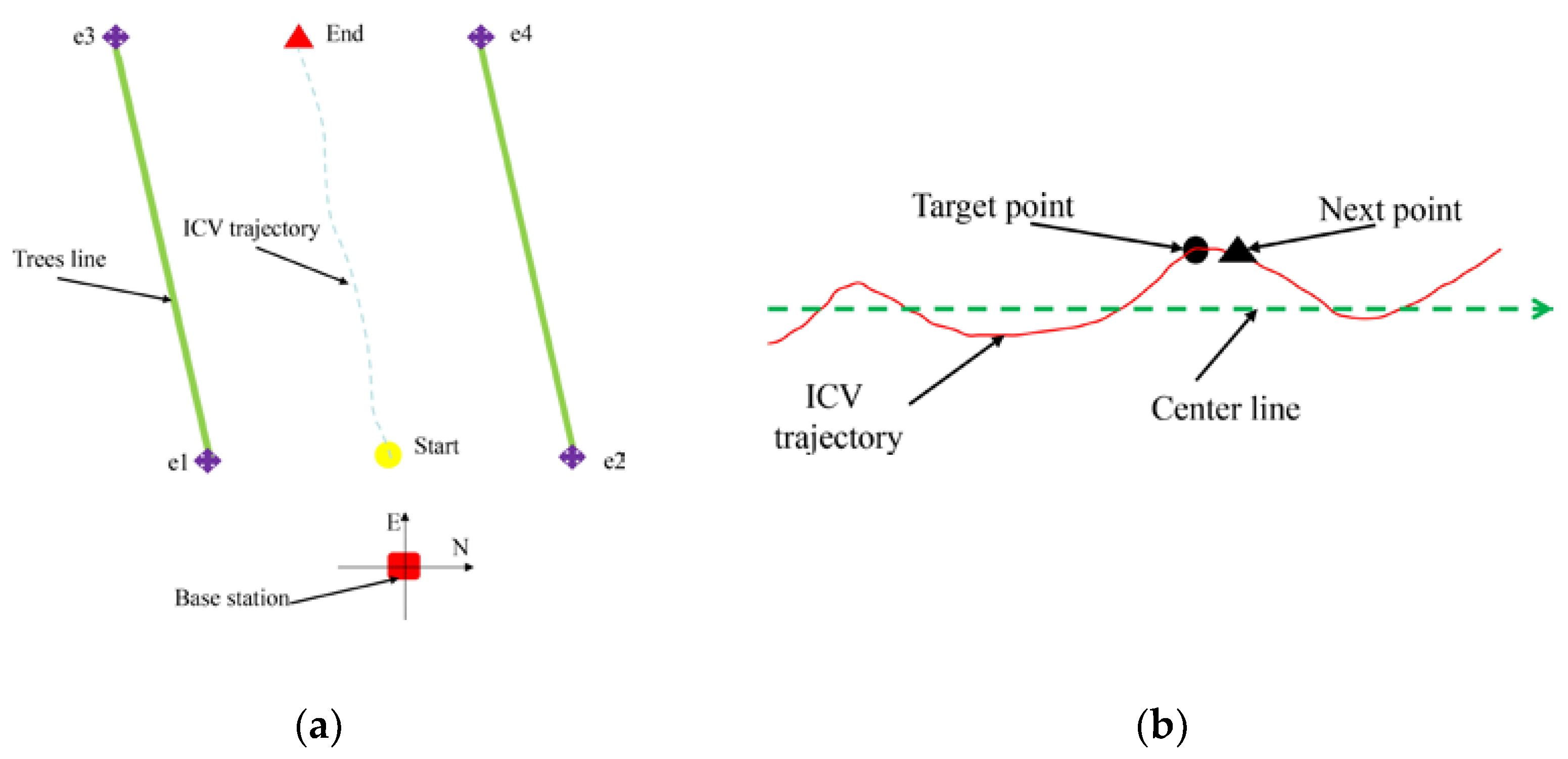
The heading angle of the ICV is obtained by real-time GPS trajectory and the center line of the tree row (Figure 8b), and the equation for the center line of the tree row can be obtained as follows:
where, e1(, ), e2(, ) are the initial coordinates of the boundaries of the boundary of the experimental area on both sides, respectively; e3(, ), e4(, ) are the end coordinates, respectively.
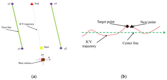
Figure 8.
Schematic diagram of positioning and heading angle measurement methods. (a) Schematic diagram of the positioning test. (b) Calculation method of heading angle.
Further simplification can be obtained:
From this, it can be seen that the slope of the center line of the tree row ( = /). We assume the current coordinates of the ICV are (x0, y0) and the coordinates of the next moment are (x0n, y0n). Consequently, the slope obtained from the two points should be = (y0n − y0)/(x0n − x0), and it can be seen that the heading angle () of the current ICV is:
2.5.2. Vertical Coordinates of Canopy Body Centers
To verify the accuracy of obtaining the vertical coordinates of the canopy body center, the vertical position of the canopy body center was compared with the value (stump positions) obtained by GPS. The experiment is repeated 5 times.
2.5.3. Canopy Length
A meter ruler with an accuracy of ±1 cm was used to measure the maximum length of the canopy of each tree on both sides of the test area. The data were measured 5 times and recorded in a notebook. The maximum length of the canopy was obtained by 4 positioning methods and 3D LiDAR calculations. The acquired lengths were compared with the lengths obtained from manual measurements to obtain the relative error of the canopy maximum length measurements. The experiment was repeated 5 times. And the canopy point cloud of group 4 with significant errors was selected for analysis.
2.5.4. Orchard Validation
To verify the high-precision positioning of method D at the inter-row canopy, the experiment was carried out in a 4-year-old cherry orchard (Figure 7c, 0.91 ha) at Shangzhuang Experimental Station of China Agricultural University (116.1923° E, 40.1478° N) in Haidian District, Beijing, with good GPS signal. The height of cherry trees is 2.95 m, with an average canopy length of 1.12 m, a plant spacing of 1.5 m, an average canopy length of 1.16 m, and a row spacing of 4 m. The selected test area is 30 m and contains 40 cherry trees. Six cherry trees at the end point are selected for the data analysis. The positioning and canopy length measurement accuracy of the 4 positioning methods at the inter-row canopy is obtained, and the experiment is repeated 5 times. The experiment was conducted on 25 October 2021. During the experiment, the weather was continuously rainless, the daytime temperature was kept at 20.6–30.4 °C, and the wind speed was lower than 1.2 m/s.
2.6. Data Processing
To facilitate the processing of the positioning data, the positioning errors of method D are compared directly using combined positioning (GPS positioning and self-positioning) and GPS positioning. Therefore, the maximum lateral positioning deviation at the inter-row single canopy for method D is roughly defined:
where, is the maximum positioning deviation at the inter-row single canopy; is maximum lateral positioning deviation between rows; and is the number of trees in the experimental area.
In the study, the deviation between measured data and actual data is represented by error (Equation (13)). In this case, both positioning deviation and heading deviation are obtained through the Equation.
where, is the error; is the measured value; is the actual value; is the number of calculations, which is taken as 25.
Given the variation of the measured positioning, the relative error (Equation (14)) can better represent the accuracy of the measured results.
where, is the relative error, %.
The canopy point clouds are displayed using Open3D 0.11.0 (Intel Inc., Santa Clara, CA, USA) by Python 3.8. The collected data were analyzed using SPSS Statistics Version 20 (IBM Inc., Armonk, NY, USA) for Windows, and plotted using OriginPro Version 2020 (OriginLab Inc., Northampton, MA, USA). All the test results were tested for normal distribution using SPSS and conformed to normal distribution.
Duncan’s post-hoc test was performed on the measured results using SPSS one-way analysis of variance (ANOVA) with a significance level of 0.05. In all cases, Duncan‘s post-hoc test was used to compare the positioning deviation, positioning relative error and the average value of the maximum canopy length of the 4 positioning methods at the 0.05 significance level.
3. Results
3.1. Motion Trajectories Obtained by the Four Positioning Methods
There are differences between the motion trajectories obtained by the four methods and the actual trajectory of the ICV obtained by GPS (Figure 9). The actual motion trajectory of the ICV is not a straight line due to the level of the operator and the ground conditions. The motion trajectories obtained by the four positioning methods are inferred relative positioning trajectories. Among them, method A only uses an encoder for position estimation of the motion trajectory, resulting in significant errors. This makes its trajectory differ from the actual trajectory. Methods B and C fuse the data from IMU and encoder for position estimation of motion trajectory, with relatively small errors. This makes its trajectory similar to the actual trajectory. Method D only performs position estimation and pose correction at the inter-row canopy, so its trajectory has a high similarity to the actual trajectory. There were significant differences between the actual trajectories of the ICV and methods A, B and C, but the differences with the method D were not significant. The actual trajectory of the ICV within the inter-row lateral distance (X-axis) of 2 m is almost the same as its motion trajectory obtained by the four positioning methods. It indicates that the positioning accuracy of the relative positioning sensor is high in a short time. As the inter-row lateral distance further increases, methods A, B, and C exhibit significant positioning deviations compared to the actual trajectory. Among them, method A showed significant positioning deviation in both inter-row lateral and vertical positioning (Y-axis). It has the largest positioning deviation. In addition, method C has a high positioning accuracy. It indicates that the EKF fusion positioning algorithm can maintain high positioning accuracy for a long time. Method D has the smallest positioning error. It indicates that method D has the highest positioning accuracy.
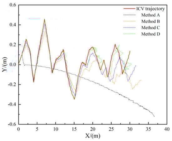
Figure 9.
Trajectories of the ICV obtained by the four methods. The figure clearly illustrates the actual trajectory of the ICV and the measured trajectories of the four methods. The X-axis represents the inter-row lateral distance and the Y-axis represents the inter-row vertical distance.
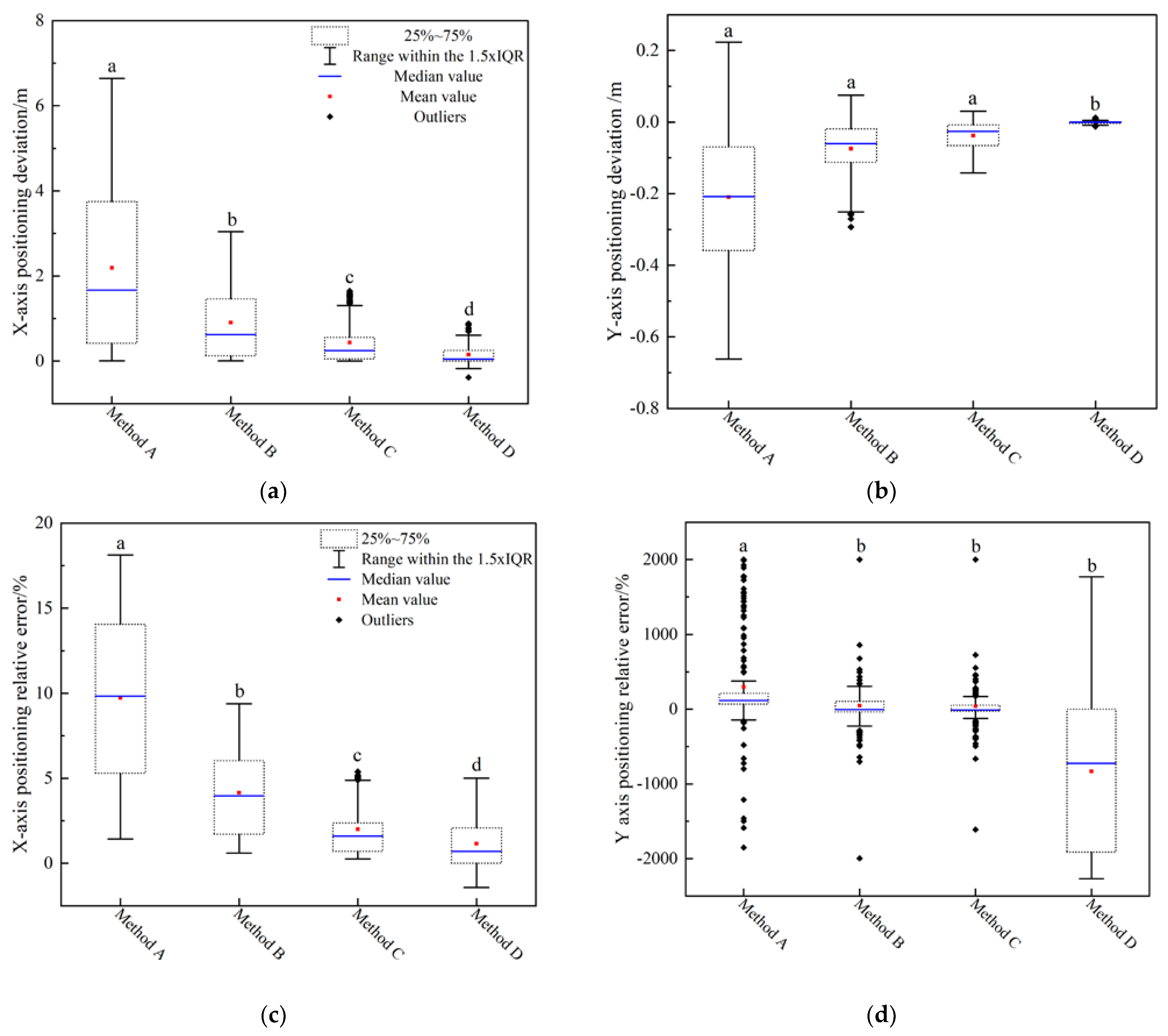
3.2. Deviation and Relative Error of Positioning
Although the ICV-measured trajectories of the four methods can be clearly obtained in Figure 9, the positioning deviations and relative errors between them and the actual trajectories cannot be quantitatively described. As far as the deviation and relative error of lateral distance positioning are concerned, there were significant differences among the four methods (Figure 10a,c). The mean positioning deviation and relative positioning error of method A (2.19 m, 10.58%), B (0.91 m, 4.80%), C (0.44 m, 2.32%), and D (0.15 m, 0.68%) decreased sequentially (Figure 10a,c). The maximum positioning deviation and relative error of methods A (6.65 m, 18.12%), B (3.04 m, 9.39%), C (1.64 m, 5.39%), and D (0.88 m, 5.02%) also decrease sequentially (Figure 10a,c). The maximum lateral positioning deviation at the inter-row canopy was calculated to be 0.22 m for method D ((Equation (12)). In terms of inter-row vertical positioning deviation, there is a significant difference between method D and the other three methods (Figure 10b). The average positioning deviation of method D is the smallest (0.05 m), with lower significance than methods A (0.66 m), B (0.29 m), and C (0.14 m). In terms of the relative error of inter-row vertical positioning, there is a significant difference between method A and the other three methods (Figure 10d). The average relative error of method A (298.35%) was the largest, which was significantly higher than that of method B (47.69%), C (39.27%) and D (−2.08%). After removing outliers, the average relative errors of methods A, B, C, and D were 40.37%, 24.45%, 16.86%, and −1.82%, respectively.
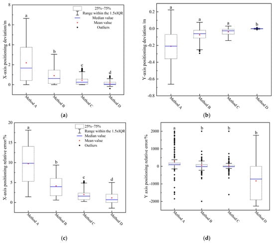
Figure 10.
Plots of the ICV positioning errors obtained by the four methods. (a) Inter-row lateral positioning deviation; (b) Inter-row vertical positioning deviation; (c) Relative error of inter-row lateral positioning; (d) Relative error of inter-row vertical positioning. For convenience of drawing, the values of method D in (d) were enlarged by 400 times. If the absolute relative error of methods A, B, and C is greater than 2000%, it should be equal to ±2000%. Different letters indicate significant differences (Duncan test, α = 0.05).
3.3. Heading Deviation
The maximum heading deviation for methods A, B, C and D were 25.4°, 66.4°, 32.75° and 4.35°, respectively. Among them, method D has the smallest heading deviation and the standard deviation (Table 1). It indicates that the method D has a significant correction for heading deviation.

Table 1.
Statistical data of heading deviation of the four positioning methods/°.
3.4. Body Center Vertical Coordinates
As shown in Figure 11, the canopy body centers (red points) of a certain plant were obtained, whereas green points represent the canopy point cloud. From the figure, it can be seen that the obtained partition canopy body centers are basically on the same plane and distributed relatively evenly. The relative error of the measured body center vertical distance is 2.36 ± 0.57%, indicating that this algorithm has high accuracy.
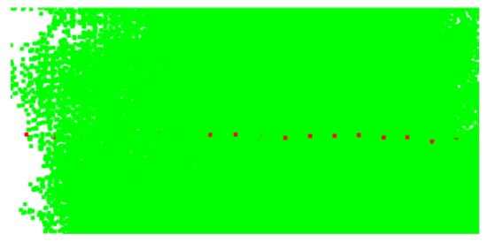
Figure 11.
Acquisition of body center locations. Green points in the figure represent the canopy and red points indicate the partitioned canopy body centers.
3.5. Relative Error of Maximum Canopy Length Measurement
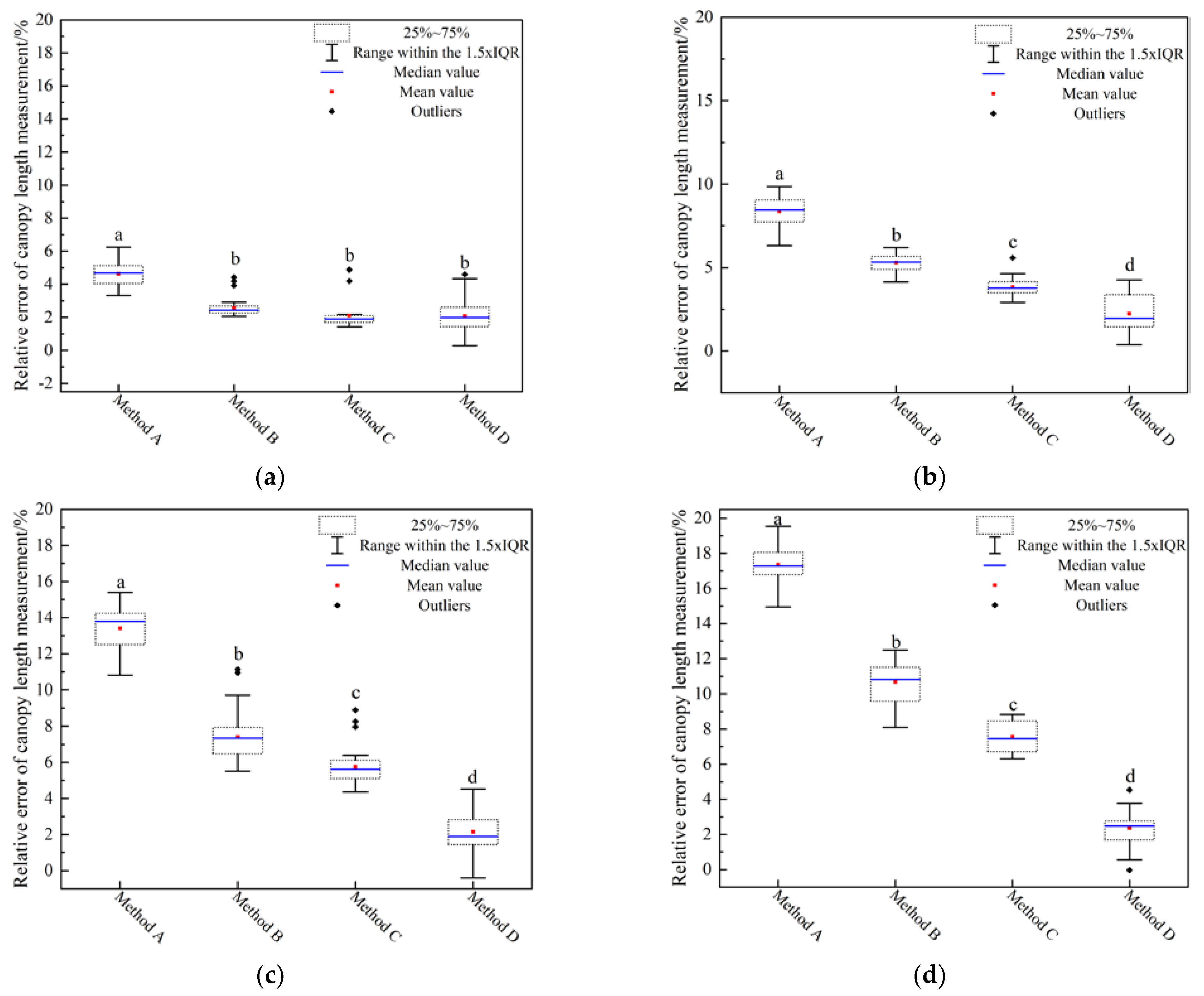
3.5.1. Relative Error of Maximum Canopy Length Measurements for the Four Positioning Methods
The relative measurement error of canopy length for methods A, B, and C increases with the increase of inter-row lateral distance, whereas the change was not significant for method D (Figure 12). In canopy group 1, the mean relative error of maximum canopy length measured by method A (4.63%) was significantly higher than that of methods B (2.57%), C (2.10%) and D (2.08%). The maximum relative measurement errors for methods A, B, C, and D were 6.24%, 4.42%, 4.89%, and 4.59%, respectively, and the difference was small. At canopy groups 2, 3, and 4, the relative errors (2.23, 2.15, and 2.36%) of canopy length measured by method D were significantly lower than those of methods A (8.37, 13.40, and 17.36%), B (5.30, 7.95, and 10.67%), and C (3.85, 5.76, and 7.57%) (Figure 12b–d). In canopy group 2, the maximum relative measurement errors of the four methods were 9.85%, 6.21%, 5.59%, and 4.26%, respectively. At this time, the relative measurement errors of method A are relatively large, while the relative measurement errors of methods B and C increase compared to method D (Figure 12b). With the further increase in traveling distance, when the ICV traveled to canopy group 3, their maximum measurement errors were 15.39%, 11.13%, 8.89% and 4.36%, respectively. At this time, the four methods are significantly different (Figure 12c). In canopy group 4, the maximum relative measurement errors were 19.54%, 12.49%, 8.84%, and 5.68%, respectively (Figure 12d).
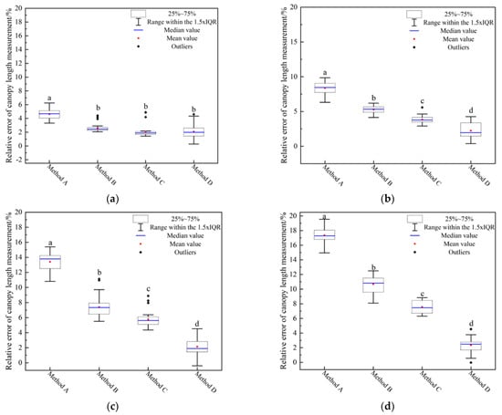
Figure 12.
Relative measurement errors of canopy length obtained by the four methods. (a) Group 1; (b) Group 2; (c) Group 3; (d) Group 4. The nearest distance from the initial point is the group 1, and the nearest distance from the end point is the group 4. Different letters indicate significant differences (Duncan test, α = 0.05).
3.5.2. Relative Errors of Maximum Canopy Length Measurements for the Four Positioning Methods
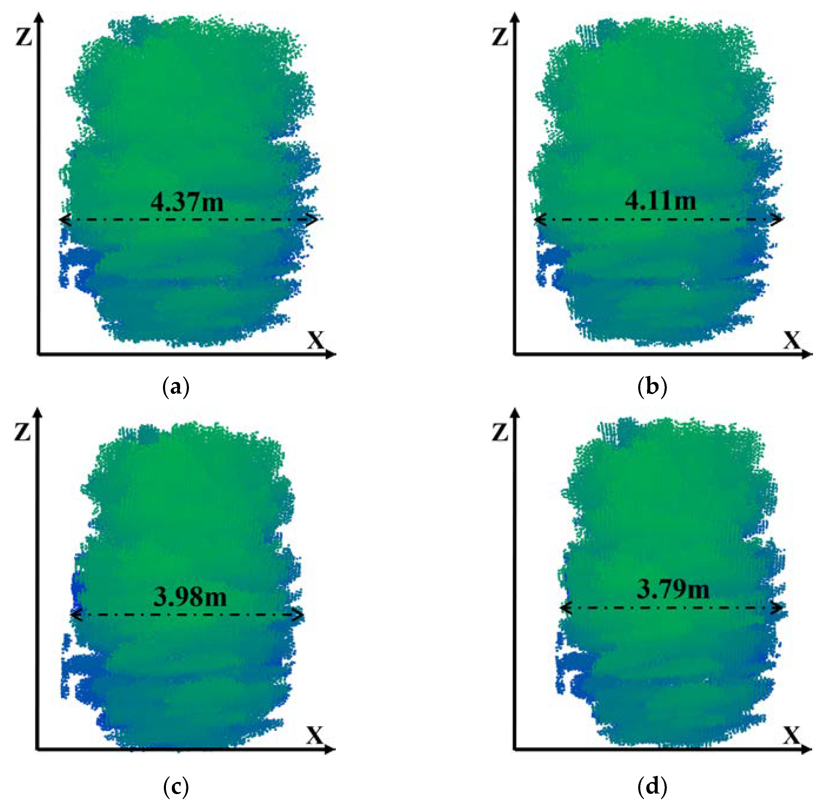
The maximum canopy lengths measured by the four positioning methods were not consistent (Figure 13). Among them, the maximum (Figure 13a, 4.37 m) was obtained by method A and the minimum (Figure 13d, 3.79 m) by method D. The maximum lengths of the canopy obtained by methods B and C were 4.11 m (Figure 13c) and 3.98 m (Figure 13d), respectively. The relative errors of the maximum length of the canopy measured by methods A, B, C and D were calculated to be 18.75%, 11.68%, 8.15% and 2.99%, respectively. It indicates that method D does not increase with increasing distance traveled in terms of measuring canopy length.

Figure 13.
Point clouds of group four ginkgo tree canopy obtained by the four methods. (a) Method A; (b) Method B; (c) Method C; (d) Method D. The X-axis represents the direction of the ICV, and the Z-axis represents vertical ground upward. The actual measured maximum canopy of the ginkgo tree was 3.69 m.
3.6. Orchard Experiment
The relative error of the positioning and the canopy measurement were calculated by removing outliers (Table 2). The positioning and maximum length of the canopy measured by the four methods were significantly different. The inter-row lateral and vertical positioning deviations (8.73 ± 2.53 m, 2.45 ± 0.91 m) and relative positioning errors (32.55 ± 9.43%, 52.35 ± 19.55%) were significantly higher in method A than those in methods B, C, and D. Among them, the inter-row lateral and vertical distances positioning deviations (0.31 ± 0.11 m, 0.15 ± 0.08 m) and relative positioning errors (4.07 ± 1.81%, 3.27 ± 1.27%) of method D were the lowest. Accordingly, method A has the worst positioning effect, whereas method D has the best positioning effect. The lateral positioning relative error of method D is lower than the vertical positioning relative error, which is different from other methods. Besides, the heading deviation (6.75 ± 1.89°) and the relative error (4.35 ± 1.09%) of canopy length measurement of method D were significantly lower than those of methods A, B and C.
Table 2.
Positioning statistics of the four positioning methods. The table includes the relative errors of the ICV’s positioning, heading and canopy measurements in the orchard.
4. Discussion
In this study, an EKF fusion positioning method (method D) based on 3D LiDAR detection correction is presented. The vertically installed 3D LiDAR (Figure 7b,d) was used to detect the presence or absence of the canopy. Based on this, it (method D) starts or closes the EKF fusion positioning method (method C) and relative positioning sensors (encoder and IMU). The inter-row initial heading and vertical position of method D were obtained through fixed row spacing and body canopy center (Figure 5 and Figure 6). The restarted method C provides the value of 0 for the initial lateral coordinates (Figure 5 and Figure 6). Consequently, the initial position of the method D is provided. It can take advantage of the short time positioning accuracy of relative positioning methods and sensors [12,35,36]. This characteristic was also demonstrated in this study (Figure 9). Furthermore, the lateral distance is corrected by the inter-row heading and vertical position acquired by 3D LiDAR. Hence, method D can accurately obtain the positioning at the inter-row canopy and the maximum length of the canopy (Figure 10, Figure 12 and Figure 13).
Since the IMU and encoder have inherent errors, the error of positioning methods cannot be eliminated and accumulates with time (driving distance) [36,37]. This is the reason why the deviations of positioning methods A, B, C and D gradually increase with time (Figure 9). Methods C and D utilize the advantageous information of encoders and IMU, which have high positioning accuracy for a longer time (Figure 9 and Figure 10) [34]. This is consistent with the findings of Cui et al. [38]. Although the sensor signals of the relative positioning method are less susceptible to receiving interference, they cannot sense the surroundings to correct the ICV position and pose [39]. The method requires a precise initial position, and usually only one [12,37]. With the increase in driving time, the error gradually accumulates, which will cause significant positioning errors [12]. Therefore, researchers have integrated positioning sensors such as machine vision, ultrasonic and sensors LiDAR into relative positioning methods [12,40,41]. It will provide fusion positioning for relative positioning methods, thereby improving positioning accuracy. However, such methods require large computational power [22].
On the basis of vertically installing 3D LiDAR to detect plant information, we also use the single 3D LiDAR to assist in positioning. It not only requires determining gaps, but also obtaining canopy information. The heading and vertical positioning at the inter-row canopy are obtained. As a result, the accuracy of inter-row heading and vertical positioning can be significantly improved (Table 1, Figure 10b). The acquisition of accurate inter-row vertical distance is a prerequisite for correcting the above parameters. The real-time canopy body center acquisition method proposed in this study has high accuracy (Figure 11). The inter-row vertical distance obtained by 3D LiDAR and lateral distance obtained by method C are both implemented on a plane. The ICV tilts or vibrates when the terrain is rough and bumpy. This can cause large errors in the calibration of method D and the lateral positioning of method C. This is the reason why the relative error of inter-row vertical positioning is negative for method D and positive for the others (Figure 10d). It is also the reason why the relative positioning error of the X-axis and Y-axis in the orchard experiment is larger than that of the sidewalk (Table 2, the length of the experimental area is consistent). Even so, method D had high positioning accuracy and canopy measurement accuracy in the orchard experiments.
Method D can provide multiple accurate initial positions within the experimental area. As a consequence, the canopy length measurements relative errors for the four groups’ canopy of method D are not significantly different, whereas those of methods A, B, and C increased with increasing inter-row lateral distance (Figure 12 and Figure 13). The maximum lateral positioning deviation at the inter-row canopy of a single tree calculated by Equation (12) is 0.22 m. The maximum canopy length obtained by method D is 0.1 m larger than the actual crown length (Figure 13d). It indicates that the calculation method for the maximum inter-row lateral positioning deviation at the canopy of a single tree is feasible. In addition, the maximum canopy lengths of the ginkgo trees (average maximum canopy length of 3.52 m) and the three cherry trees (average maximum canopy length of 1.16 m) on campus were essentially the same. But the lateral positioning error at the inter-row canopy of the ginkgo trees on campus was smaller than cherry trees. It indicates that the topography of the orchard has a significant impact on both positioning and canopy measurement accuracy.
In summary, it can be seen that high-precision positioning at the inter-row canopy is a prerequisite to ensure the accuracy of canopy length measurement. Yet, method D has significant limitations. It can only be used in orchards (planted forests) with fixed row spacing and large gaps and young or sparse orchards (planted forests). In the future, the gap above a standardized planted 3D crop could be utilized to close or start method C. Fixed row spacing is utilized through method D to provide inter-row heading and vertical positioning to extend the method use. Meanwhile, it is necessary to introduce the ICV roll angle to correct the point cloud and further improve positioning accuracy. Where the GNSS signal is good, its signal is incorporated into the method to provide accomplished positioning information. Moreover, the method is used to modify the existing manned and remote-controlled sprayers into precision variable-rate sprayers, providing new vitality for the old machines. Although it has achieved good positioning and canopy length measurement accuracy, it can only be used as an auxiliary positioning rather than a conventional positioning method. It can provide new ideas for inter-row vehicle positioning and canopy length measurement methods at the canopy for variable-rate spraying in planted forests and orchards. Additionally, the method is drawn upon to solve the problem of low positioning and canopy length measurement accuracy in agricultural surroundings with poor GPS signals.
5. Conclusions
The kinematics and measurement models of the ICV were constructed by IMU and encoder. The EKF fusion positioning method (method C) is designed by fusing the sensor data using the EKF filtering algorithm. The 3D LiDAR is fused into method C to achieve the EKF fusion positioning method (method D) based on 3D LiDAR detected correction. Method D eliminates the cumulative errors of the IMU and the encoder by closing gaps or starting method C at inter-row canopies. Furthermore, 3D LiDAR provides initial heading and inter-row vertical through body center and fixed row spacing and assists in positioning. As a result, the accuracy of inter-row positioning and canopy length measurement can be greatly improved. From the campus and orchard experiments and discussions, it can be concluded that:
- (1)
- In the campus test area, the positioning at the inter-row canopy for method D is relatively small and does not increase with inter-row travel distance. The lateral positioning at the individual tree canopies increased with the increase in driving distance. Among them, the deviation of inter-row lateral and vertical positioning at the canopy was less than 0.22 m and 0.15 m, respectively, the heading deviation was less than 4.35°, and the relative error of canopy length measurement was less than 5.68%. It indicates that the method has high positioning accuracy on flat terrain.
- (2)
- The orchard experiments showed that the positioning deviations were larger than those on the campus due to the influence of orchard terrain or mechanical vibration. Hence, the average inter-row lateral and vertical positioning deviations at the canopy were 0.1 m and 0.2 m, the average heading deviation was 6.75°, and the average relative error of canopy length measurement was 4.35%. It indicates that the positioning accuracy of the method is still very high on rugged terrain.
- (3)
- The method is suitable for 3D crops with standardized planting and gaps between canopies, which has significant limitations. The method can solve the problem of low accuracy of positioning and canopy length measurement in 3D crops with poor GPS signals. It has great potential for application.
Although the method proposed in this study solves the problem of inter-row canopy positioning and canopy measurement, there are still many problems. We will use IMU to acquire the rolling angle of the vehicle and improve the accuracy of 3D LiDAR to acquire the vertical coordinates of the body center. Moreover, the accuracy of method C in different terrains will be improved based on the acquired rolling angle. In addition, method D is extended from 2D to 3D to address many problems in actual operations. Furthermore, the method is applied to other crops with fixed row spacing, and gaps in the upper canopy, such as tomatoes in greenhouses.
Author Contributions
Conceptualization, L.L., S.W. and Z.Z.; methodology, L.L. and D.J.; software, L.L. and D.J.; validation, S.W. and Z.Z.; formal analysis, L.L., S.W. and Z.Z.; investigation, L.L., D.J., F.Z. and Z.Z.; resources, S.W. and Z.Z.; data curation, L.L., D.J., F.Z. and Z.Z.; writing—original draft, L.L., D.J., S.W. and F.Z.; visualization, L.L. and F.Z.; and funding Z.Z., S.W. and L.L.; acquisition, Z.Z. All authors have read and agreed to the published version of the manuscript.
Funding
This work was supported by Program for Innovative Research Team in SDAEU (sgykycxtd2020-03), and CCF- Baidu Apollo Joint Development Project Fund.
Data Availability Statement
The original contributions presented in the study are included in the article, further inquiries can be directed to the corresponding author.
Acknowledgments
The authors would like to give special thanks to Tian Zhong for providing the test orchard.
Conflicts of Interest
The authors declare no conflict of interest.
Appendix A
Appendix A.1. Error Sources and Calibration of Encoder
A rotary encoder is a sensor used to measure rotation angle, speed, and direction, which converts angular displacement or angular velocity into a series of electrical digital pulses. The incremental encoder is used in this study. Although incremental rotary encoders have many advantages, they are driven by mechanical transmission to rotate the encoder disk. It makes the encoder highly susceptible to mechanical vibration, resulting in the generation of burrs that affect the number of pulses generated. This ultimately leads to significant measurement errors. To ensure the computing power of the microcontroller, the use of software methods to improve the measurement accuracy of the encoder is abandoned. On the contrary, we used the encoder mode designed by ST company for the STM32 microcontroller. The method utilizes hardware to improve the measurement accuracy of the encoder used in this study.
The counting methods of the encoder mode are shown in Table A1, which are divided into three modes: counting only at TI1 (mode 1), counting only at TI2 (mode 2), and counting both at TI1 and TI2 (mode 3). When the encoder rotates forward, regardless of the mode, the count value increases. Similarly, when reversing, the count values are decreasing.
Table A1.
Relationship between counting direction and signal.
Table A1.
Relationship between counting direction and signal.
| Active Edge | Level of Opposite Signals * | TI1FP1 Signal | TI2FP2 Signal | ||
|---|---|---|---|---|---|
| Increase | Decrease | Increase | Decrease | ||
| Count only at TI1 | High | — | + | \ | \ |
| Lower | + | — | \ | \ | |
| Count only at TI2 | High | \ | \ | + | — |
| Lower | \ | \ | — | + | |
| Count at both TI1 and TI2 | High | — | + | + | — |
| Lower | + | — | — | + | |
Note: * TI1FP1 corresponds to TI2, and TI2FP2 corresponds to TI1. “+” Indicates an increasing count; “—” Indicates a decrease in count; “\” Indicates no counting.
From the three counting modes mentioned above, it can be seen that mode 1 and mode 2 are counting at 2 times the frequency, while mode 3 is counting at 4 times the frequency. As shown in Figure A1, the encoder generates four counts for every pulse counter generated, while effectively removing the impact caused by dithering. Compared to the other modes, mode 3 can better remove burrs and interference. Therefore this study chooses mode 3.
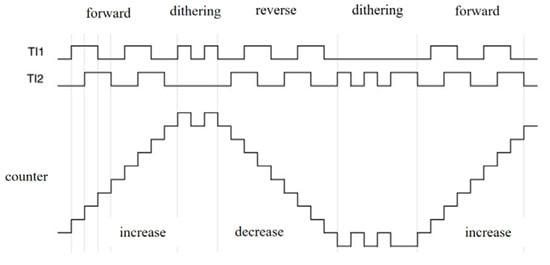
Figure A1.
Counter schematic for encoder mode 3.
Figure A1.
Counter schematic for encoder mode 3.

A comparison test was conducted using the number of pulses captured by A-phase and microcontroller external interrupts alone (method 1), and the number of pulses captured by the encoder software 4× technique (method 2) with the present method (method 3). This experiment was conducted five times, with eight measurements taken each time. One-way ANOVA analysis (Wall Duncan’s test) was performed using SPSS 26.0, and the results are shown in Table A2. The relative errors of the three methods were significantly differences, with method 1 having a relative error of approximately 4 times that of method 2. Compared to method 2, method 3 has a smaller relative error, indicating that encoder mode 3 has a good burr removal effect.
Table A2.
Relative Error of Three Measurement Methods.
Table A2.
Relative Error of Three Measurement Methods.
| Measuring Method | Method 1 | Method 2 | Method 3 |
|---|---|---|---|
| Data | 8.56 ± 0.73 a | 2.23 ± 0.21 b | 0.19 ± 0.03 c |
Note: The data in the table are described using mean and standard deviation, with different letters indicating significant differences at the 0.05 level.
Appendix A.2. Error Sources and Calibration of IMU
Due to production and processing reasons, IMUs are highly susceptible to factors such as installation, zero drift, and random noise. In addition to the aforementioned sources of error, scaling errors may also occur due to inconsistent physical parameters of components on magnetometers, accelerometers, and gyroscopes. In addition, sensors may experience certain drift and accumulate errors during long-term use. To improve measurement accuracy, it is necessary to calibrate the parameters of the geomagnetic pole and gyroscope before using them.
The accelerometer is in a stationary state, and each attitude is only affected by gravity. In three-dimensional space, the gravity points are all on a spherical surface. However, there may be deviations in the measurement units between the axes, and the gravity points of each attitude fall on an ellipsoid. The center of the ellipsoid is the offset of the acceleration, which is the calibration value. The magnetometer senses the same magnetic field intensity for each attitude in a constant environment, so there is no need to measure the magnetic field intensity in a stationary state. Instead, it is slowly rotated along the three axes, which ensures a more uniform distribution of the collected spatial attitude data from the magnetometer.
Due to the presence of errors, the measurement data of accelerometers and magnetometers will be distributed on an ellipsoid that is not centered around the zero point. The calibration process is the process of fitting the ellipsoid, and the model of the ellipsoid is as follows:
Because of the presence of errors, the measurement data of accelerometers and magnetometers will be distributed on an ellipsoid that is not centered around the zero point. The calibration process is the process of fitting the ellipsoid, and the model of the ellipsoid is as follows:
According to the ellipsoid fitting equation, there are six unknown variables, where (, , ) is the fitted ellipsoid center and also the zero bias on the accelerometer or gyroscope. (, , ) is the scaling factor on the three axes, and the above equation can be simplified into:
The center of the ellipsoid and the scale factor of the required solution, as well as , , , , and have the following relationship:
To obtain the values of , , , , and , samples of 7 or more magnetometers and accelerometers need to be measured. By inputting their values into Equation (A3), the calibrated error parameters of the magnetometer and accelerometer can be obtained.
This study uses PyCharm 2022 and Python 3.8 programming to collect data from accelerometers in a stationary state and magnetometers in a moving state. We use the above equation to solve for their ellipsoidal center coordinates and ellipsoidal radius lengths. As shown in Table A3, the center and half-axis lengths of the ellipsoids of the accelerometer and magnetometers obtained are similar. Among them, the half-axis lengths of the three ellipsoids of the magnetometer are not significantly different, and the fitted ellipsoids obtained are basically consistent with those of the sphere (Figure A2b). The length of the a and b axes of the accelerometer in this IMU is basically the same. The length of the c-axis is about 10 times that of the first two. The fitted shape is similar to a rugby (Figure A2a). From this, it can be seen that due to the presence of bias and error, the ellipsoidal centers of the accelerometer and magnetometers are not on the original (0 g, 0 g, 0 g) and (0, 0, 0). It is necessary to transfer the centers of each ellipsoid to the original center for correction, normalize the magnetometer, and convert the coordinates of all axes to a sphere with a radius length of 72.1410. Meanwhile, normalize the a and b axes of the accelerometer while keeping the c axis unchanged.
Table A3.
Ellipsoid calibration parameters.
Table A3.
Ellipsoid calibration parameters.
| Type | Elliptical Center Coordinates | Elliptical Half-Axis Length | ||||
|---|---|---|---|---|---|---|
| a | b | c | ||||
| Accelerometer | 0.0092 g | −0.0158 g | 1.0035 g | 0.0017 | 0.0019 | 0.0117 |
| Magnetometer | −2.4917 | 1.2728 | 0.6507 | 74.9957 | 72.1410 | 72.5667 |
As shown in Figure A2, the results of ellipsoidal fitting for accelerometer and magnetometers are shown. As mentioned earlier, one is similar to rugby, whereas the other is similar to a sphere. The ellipsoidal half-axis of the accelerometer is represented by a green line, whereas the ellipsoidal half-axis of the magnetometer is represented by a yellow line.
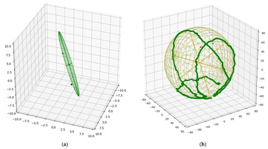
Figure A2.
Ellipsoid fitting results. (a) Ellipsoidal fitting results of the accelerometer. (b) Ellipsoidal fitting results of the magnetometer.
Figure A2.
Ellipsoid fitting results. (a) Ellipsoidal fitting results of the accelerometer. (b) Ellipsoidal fitting results of the magnetometer.
The measurement data on the three axes of the gyroscope will have zero bias due to the influence of power supply voltage and temperature. The existence of zero bias will lead to cumulative errors. This will result in a decrease in measurement accuracy, so it is necessary to calibrate the gyroscope. Place the IMU stationary on a horizontal plane, sample it, and take the average value of each axis to obtain the zero deviation on its axis.
By standing the IMU on flat outdoor ground for 1 min and using Python 3.8 programming to collect data, the entire process is repeated five times. The obtained values of , and are −1.0139, 1.2950, and 0.000030371 rad/s, respectively.
Appendix B
Appendix B.1. A Positioning Method Based on EKF
We use the EKF algorithm to fuse the data measured by IMU and encoder, and obtain real-time position estimation, prediction, and measurement.
Appendix B.2. Prediction and Observation Equations Based on EKF
EKF is an optimal estimate for linear Gaussian systems. However, in many positioning problems, state transformation and measurement are both nonlinear. EKF takes a first-order approximation for this nonlinear system using Taylor expansion. Then they use EKF to complete state estimation. Assuming that the prediction and observation equations of ICV are both nonlinear systems, the EKF algorithm is as follows:
where, and represent the states of the ICV at moment and moment, respectively; is the observed values of the ICV at moment; and are respectively state (process) noise and observation (measurement) noise; Both of them follow a Gaussian distribution or normal distribution; is the input control variables within moment to moment; and are the state transition matrix and observation matrix, respectively.
Expanding in Equation (A5) using Taylor equation at the mean of moment, taking a first-order approximation, we can obtain:
Meanwhile, the in Equation (A6) is expanded using the Taylor equation at the predicted mean , and taking a first-order approximation can obtain:
In Equations (A6) and (A7), and are Jacobian matrices:
Appendix B.3. Encoder and IMU Fusion Positioning Method Based on EKF
Based on the prediction and observation equations mentioned above and the principle of the EKF algorithm, the steps of the EKF algorithm using IMU and encoder are further obtained. The specific details are as follows:
The first step is to predict the motion state of ICV:
where, and represent the mean and variance of the state prediction; is process noise, it conforms to a normal distribution.
Simultaneously update the measured ICV motion status:
where, and represent the mean and variance of the state prediction; is process noise, it conforms to a normal distribution. is the Kalman gain; is measure noise; and are the mean and variance of the EKF, respectively; is unit matrices
In this study, the specific process of the measurement data fusion algorithm for two positioning sensors based on EKF will be described in the following. Assuming the motion state of ICV at moment is . The mean state at moment is , its state vector is Equation (1) in the formal manuscript. By incorporating the motion model Equation (2) into the ICV, the mean predicted state in Equation (A10) can be obtained as:
By taking the derivative of Equation (2) in the formal manuscript over in sequence, the Jacobian matrix can be obtained as:
The expression for and are as follows:
At this time, according to the EKF algorithm, the covariance () of the predicted state of ICV can be obtained by incorporating Equation (2) and process noise into Equation (1). However, the measurement error of the two positioning sensors is relatively large. If one is used for prediction and the other is used for correction, there will still be significant deviation in the position and attitude of the fused positioning. Therefore, combining the motion model of ICV with its motion state as prediction, and using the data from both sensors (the average of both) as measurement models. When the measurement error of one sensor is large, choose other measurement data.
References
- Chowdhury, M.; Thomas, E.V.; Jha, A.; Kushwah, A.; Kurmi, R.; Khura, T.K.; Sarkar, P.; Patra, K. An Automatic Pressure Control System for Precise Spray Pattern Analysis on Spray Patternator. Comput. Electron. Agric. 2023, 214, 108287. [Google Scholar] [CrossRef]
- Rogers, H.; De La Iglesia, B.; Zebin, T.; Cielniak, G.; Magri, B. An Automated Precision Spraying Evaluation System. In Proceedings of the Lecture Notes in Computer Science (Including Subseries Lecture Notes in Artificial Intelligence and Lecture Notes in Bioinformatics), Cambridge, UK, 5–8 September 2023; Volume 14136 LNAI. [Google Scholar]
- Kolendo, Ł.; Kozniewski, M.; Ksepko, M.; Chmur, S.; Neroj, B. Parameterization of the Individual Tree Detection Method Using Large Dataset from Ground Sample Plots and Airborne Laser Scanning for Stands Inventory in Coniferous Forest. Remote Sens. 2021, 13, 2753. [Google Scholar] [CrossRef]
- Wu, H.; Wang, S. Design and Optimization of Intelligent Orchard Frost Prevention Machine under Low-Carbon Emission Reduction. J. Clean. Prod. 2023, 433, 139808. [Google Scholar] [CrossRef]
- Li, L.; He, X.; Song, J.; Wang, X.; Jia, X.; Liu, C. Design and Experiment of Automatic Profiling Orchard Sprayer Based on Variable Air Volume and Flow Rate. Nongye Gongcheng Xuebao/Trans. Chin. Soc. Agric. Eng. 2017, 33, 70–76. [Google Scholar]
- Qin, J.; Wang, W.; Mao, W.; Yuan, M.; Liu, H.; Ren, Z.; Shi, S.; Yang, F. Research on a Map-Based Cooperative Navigation System for Spraying–Dosing Robot Group. Agronomy 2022, 12, 3114. [Google Scholar] [CrossRef]
- Gao, Z.-Q.; Zhao, C.-X.; Cheng, J.-J.; Zhang, X.-C. Tree Structure and 3-D Distribution of Radiation in Canopy of Apple Trees with Different Canopy Structures in China. Chin. J. Eco-Agric. 2012, 20, 63–68. [Google Scholar] [CrossRef]
- Khemira, H.; Schrader, L.E.; Peryea, F.J.; Kammereck, R.; Burrows, R. Effect of Rootstock on Nitrogen and Water Use in Apple Trees. HortScience 2019, 32, 486A-486. [Google Scholar] [CrossRef]
- Liu, L.; Wang, J.; Mao, W.; Shi, G.; Zhang, X.; Jiang, H. Canopy Information Acquisition Method of Fruit Trees Based on Fused Sensor Array. Nongye Jixie Xuebao/Trans. Chin. Soc. Agric. Mach. 2018, 49, 359. [Google Scholar]
- Jiang, H.; Liu, L.; Liu, P.; Wang, J.; Zhang, X.; Gao, D. Online Calculation Method of Fruit Trees Canopy Volume for Precision Spray. Nongye Jixie Xuebao/Trans. Chin. Soc. Agric. Mach. 2019, 50, 120–129. [Google Scholar]
- Lan, Y.; Yan, Y.; Wang, B.; Song, C.; Wang, G. Current Status and Future Development of the Key Technologies for Intelligent Pesticide Spraying Robots. Nongye Gongcheng Xuebao/Trans. Chin. Soc. Agric. Eng. 2022, 38, 30–40. [Google Scholar]
- Saqib, N. Positioning—A Literature Review. PSU Res. Rev. 2021, 5, 141–169. [Google Scholar] [CrossRef]
- Yao, H.; Liang, X.; Chen, R.; Wang, X.; Qi, H.; Chen, L.; Wang, Y. A Benchmark of Absolute and Relative Positioning Solutions in GNSS Denied Environments. IEEE Internet Things J. 2024, 11, 4243–4273. [Google Scholar] [CrossRef]
- Perez-Ruiz, M.; Upadhyaya, S. GNSS in Precision Agricultural Operations. In New Approach of Indoor and Outdoor Localization Systems; Intech: Houston, TX, USA, 2012. [Google Scholar]
- Jin, S.; Wang, Q.; Dardanelli, G. A Review on Multi-GNSS for Earth Observation and Emerging Applications. Remote Sens. 2022, 14, 3930. [Google Scholar] [CrossRef]
- Perez-Ruiz, M.; Martínez-Guanter, J.; Upadhyaya, S.K. High-Precision GNSS for Agricultural Operations. In GPS and GNSS Technology in Geosciences; Elsevier: Amsterdam, The Netherlands, 2021. [Google Scholar]
- de Ponte Müller, F. Survey on Ranging Sensors and Cooperative Techniques for Relative Positioning of Vehicles. Sensors 2017, 17, 271. [Google Scholar] [CrossRef]
- Mohanty, A.; Wu, A.; Bhamidipati, S.; Gao, G. Precise Relative Positioning via Tight-Coupling of GPS Carrier Phase and Multiple UWBs. IEEE Robot. Autom. Lett. 2022, 7, 5757–5762. [Google Scholar] [CrossRef]
- Teso-Fz-Betoño, D.; Zulueta, E.; Sanchez-Chica, A.; Fernandez-Gamiz, U.; Teso-Fz-Betoño, A.; Lopez-Guede, J.M. Neural Architecture Search for the Estimation of Relative Positioning of the Autonomous Mobile Robot. Log. J. IGPL 2023, 31, 634–647. [Google Scholar] [CrossRef]
- Xia, Y.; Lei, X.; Pan, J.; Chen, L.W.; Zhang, Z.; Lyu, X. Research on Orchard Navigation Method Based on Fusion of 3D SLAM and Point Cloud Positioning. Front. Plant Sci. 2023, 14, 1207742. [Google Scholar] [CrossRef]
- Chen, B.; Zhao, H.; Zhu, R.; Hu, Y. Marked-LIEO: Visual Marker-Aided LiDAR/IMU/Encoder Integrated Odometry. Sensors 2022, 22, 4749. [Google Scholar] [CrossRef]
- Liu, H.; Duan, Y.; Shen, Y. Real-Time Navigation Method of Orchard Mobile Robot Based on Laser Radar Dual Source Information Fusion. Nongye Jixie Xuebao/Trans. Chin. Soc. Agric. Mach. 2023, 54, 249–258. [Google Scholar]
- Chen, M.; Tang, Y.; Zou, X.; Huang, Z.; Zhou, H.; Chen, S. 3D Global Mapping of Large-Scale Unstructured Orchard Integrating Eye-in-Hand Stereo Vision and SLAM. Comput. Electron. Agric. 2021, 187, 106237. [Google Scholar] [CrossRef]
- Liu, W.; He, X.; Liu, Y.; Wu, Z.; Yuan, C.; Liu, L.; Qi, P.; Li, T. Navigation Method between Rows for Orchard Based on 3D LiDAR. Nongye Gongcheng Xuebao/Trans. Chin. Soc. Agric. Eng. 2021, 37, 165–174. [Google Scholar]
- Jiang, S.; Qi, P.; Han, L.; Liu, L.; Li, Y.; Huang, Z.; Liu, Y.; He, X. Navigation System for Orchard Spraying Robot Based on 3D LiDAR SLAM with NDT_ICP Point Cloud Registration. Comput. Electron. Agric. 2024, 220, 108870. [Google Scholar] [CrossRef]
- Jiang, A.; Ahamed, T. Navigation of an Autonomous Spraying Robot for Orchard Operations Using LiDAR for Tree Trunk Detection. Sensors 2023, 23, 4808. [Google Scholar] [CrossRef] [PubMed]
- Zhang, H.; Li, X.; Wang, L.; Liu, D.; Wang, S. Construction and Optimization of a Collaborative Harvesting System for Multiple Robotic Arms and an End-Picker in a Trellised Pear Orchard Environment. Agronomy 2024, 14, 80. [Google Scholar] [CrossRef]
- Guevara, J.; Auat Cheein, F.A.; Gené-Mola, J.; Rosell-Polo, J.R.; Gregorio, E. Analyzing and Overcoming the Effects of GNSS Error on LiDAR Based Orchard Parameters Estimation. Comput. Electron. Agric. 2020, 170, 105255. [Google Scholar] [CrossRef]
- Baltazar, A.R.; Santos, F.N.D.; De Sousa, M.L.; Moreira, A.P.; Cunha, J.B. 2D LiDAR-Based System for Canopy Sensing in Smart Spraying Applications. IEEE Access 2023, 11, 43583–43591. [Google Scholar] [CrossRef]
- Jiang, S.; Wang, S.; Yi, Z.; Zhang, M.; Lv, X. Autonomous Navigation System of Greenhouse Mobile Robot Based on 3D Lidar and 2D Lidar SLAM. Front. Plant Sci. 2022, 13, 5281. [Google Scholar] [CrossRef] [PubMed]
- Liu, L.; Liu, Y.; He, X.; Liu, W. Precision Variable-Rate Spraying Robot by Using Single 3D LIDAR in Orchards. Agronomy 2022, 12, 2509. [Google Scholar] [CrossRef]
- Liu, L.; He, X.; Liu, W.; Liu, Z.; Han, H.; Li, Y. Autonomous Navigation and Automatic Target Spraying Robot for Orchards. Smart Agric. 2022, 4, 63. [Google Scholar]
- Rivera, G.; Porras, R.; Florencia, R.; Sánchez-Solís, J.P. LiDAR Applications in Precision Agriculture for Cultivating Crops: A Review of Recent Advances. Comput. Electron. Agric. 2023, 207, 107737. [Google Scholar] [CrossRef]
- Hu, F.; Wu, G. Distributed Error Correction of EKF Algorithm in Multi-Sensor Fusion Localization Model. IEEE Access 2020, 8, 93211–93218. [Google Scholar] [CrossRef]
- Zheng, W.; Gong, G.; Tian, J.; Lu, S.; Wang, R.; Yin, Z.; Li, X.; Yin, L. Design of a Modified Transformer Architecture Based on Relative Position Coding. Int. J. Comput. Intell. Syst. 2023, 16, 168. [Google Scholar] [CrossRef]
- Sagar, A.S.M.S.; Kim, T.; Park, S.; Lee, H.S.; Kim, H.S. Relative-Position Estimation Based on Loosely Coupled UWB–IMU Fusion for Wearable IoT Devices. Comput. Mater. Contin. 2023, 75, 1941–1961. [Google Scholar] [CrossRef]
- Shaw, P.; Uszkoreit, J.; Vaswani, A. Self-Attention with Relative Position Representations. In Proceedings of the NAACL HLT 2018–2018 Conference of the North American Chapter of the Association for Computational Linguistics: Human Language Technologies—Proceedings of the Conference, New Orleans, LA, USA, 1–6 June 2018; Volume 2. [Google Scholar]
- Cui, Y.; Zhang, Y.; Huang, Y.; Wang, Z.; Fu, H. Novel WiFi/MEMS Integrated Indoor Navigation System Based on Two-Stage EKF. Micromachines 2019, 10, 198. [Google Scholar] [CrossRef] [PubMed]
- He, Y.; Wu, J.; Xie, G.; Hong, X.; Zhang, Y. Data-Driven Relative Position Detection Technology for High-Speed Maglev Train. Measurement 2021, 180, 109468. [Google Scholar] [CrossRef]
- Xue, H.; Fu, H.; Dai, B. IMU-Aided High-Frequency Lidar Odometry for Autonomous Driving. Appl. Sci. 2019, 9, 1506. [Google Scholar] [CrossRef]
- Petrović, I.; Sečnik, M.; Hočevar, M.; Berk, P. Vine Canopy Reconstruction and Assessment with Terrestrial Lidar and Aerial Imaging. Remote Sens. 2022, 14, 5894. [Google Scholar] [CrossRef]


Disclaimer/Publisher’s Note: The statements, opinions and data contained in all publications are solely those of the individual author(s) and contributor(s) and not of MDPI and/or the editor(s). MDPI and/or the editor(s) disclaim responsibility for any injury to people or property resulting from any ideas, methods, instructions or products referred to in the content. |
© 2024 by the authors. Licensee MDPI, Basel, Switzerland. This article is an open access article distributed under the terms and conditions of the Creative Commons Attribution (CC BY) license (https://creativecommons.org/licenses/by/4.0/).