Climate-Informed Management of Irrigated Cotton in Western Kansas to Reduce Groundwater Withdrawals

Abstract

The Ogallala aquifer, underlying eight states from South Dakota to Texas, is practically non-recharging south of Nebraska, and groundwater withdrawals for irrigation have lowered the aquifer in western Kansas. Subsequent well-yield declines encourage deficit irrigation, greater reliance on precipitation, and producing profitable drought-tolerant crops like upland cotton (Gossypium hirsutum (L.)). Our objective was to evaluate deficit irrigated cotton growth, yield, and water productivity (CWP) in northwest, west-central, and southwest Kansas in relation to El Niño southern oscillation (ENSO) phase effects on precipitation and growing season cumulative thermal energy (CGDD). Using the GOSSYM crop growth simulator with actual 1961–2000 location weather records partitioned by the ENSO phase, we modeled crop growth, yield, and evapotranspiration (ET) for irrigation capacities of 2.5, 3.75, and 5.0 mmd⁻¹ and periods of 4, 6, and 8 weeks. Regardless of location, the ENSO phase did not influence CGDD, but precipitation and lint yield decreased significantly in southwest Kansas during La Niña compared with the Neutral and El Niño phases. Simulated lint yields, ET, CWP, and leaf area index (LAI) increased with increasing irrigation capacity despite application duration. Southwestern Kansas producers may use ENSO phase information with deficit irrigation to reduce groundwater withdrawals while preserving desirable cotton yields.

1. Introduction

The semiarid US High Plains region receives approximately 450 mm mean annual precipitation that supplies as little as 40% of the potential crop evapotranspiration (ET) in the western Great Plains [1]. The remaining ET is typically supplied by irrigation of groundwater withdrawn from the High Plains or Ogallala aquifer at rates that grossly exceed the negligible aquifer recharge [2]. The resulting change in overall saturated thickness of the High Plains Aquifer since development in the 1950s from Texas to South Dakota averages a spatially weighted decline of 4.8 m, including 8.0 m in Kansas, which was second only to a 12.5 m decline in Texas [3]. Groundwater withdrawals from the Ogallala lowered the saturated thickness in western Kansas by an average of 0.16- to 0.51 m annually over the past 20 years [4]. Counter to negligible recharge, Whittemore et al. [4] determined sustainable irrigation, defined as water withdrawals for irrigation that do not lower the water table further, would require an average 30% reduction in pumping for western Kansas. Nevertheless, Haacker et al. [5] predicted the eventual depletion of the central and southern Ogallala Aquifer by 2100, thus eliminating continued unsustainable irrigated production in affected irrigated areas. An adequate and stable water source is fundamental to all sustainable irrigated crop production, but that will require extending the longevity of the Ogallala aquifer through reduced water withdrawals that combine more efficient irrigation, drought-tolerant alternative crops, and decreased irrigated land area.

Water use on the Texas High Plains was reduced by about 2–4% with improved irrigation scheduling and application technologies to increase irrigation efficiency [6,7]. Colaizzi et al. [7] went on to state that additional water savings averaging about 8% could be achieved by producing alternate crops that better tolerate water deficit stress. Cotton is an alternative crop gaining interest in Kansas because of its similar profitability to corn (Zea mays L.) and 30% lower estimated seasonal ET [8]. Based on an empirical growing season cumulative thermal energy (CGDD) model, Gowda et al. [9] concluded that well-watered cotton was a suitable alternative crop for southwest Kansas that could reduce water use. Using mechanistic crop growth simulation, Baumhardt et al. [10] estimated average water use of deficit irrigated cotton at ~460 mm in western Kansas, which is 30% less than the ~650 mm ET value for fully irrigated corn [11,12]. The relatively small cotton yields in the northwest and west-central areas of Kansas, regardless of the irrigation level, combined with costs for non-routine production, may be insufficient for risk-averse producers to change principal crops [10].

El Niño southern oscillation (ENSO) describes atmospheric coupling to the equatorial sea surface temperatures. In the southern Great Plains of North America, ENSO is climatically manifested as being warmer and drier in the La Niña phase compared with the cooler and wetter climate of an El Niño phase or having no effect in the Neutral phase [13]. By contrast, the northern Great Plains, including Canada and the northern U.S. Plains and mountain states, experience the opposite of those climate conditions of the southern Great Plains. The impact of the ENSO phase varies seasonally as they mature near December; for example, wheat production benefits from El Niño conditions in the southern Great Plains. A greater understanding of this phenomenon has improved weather forecasts [14] and may permit climate-informed crop irrigation management, which utilizes expected growing season conditions, including precipitation, to produce wheat crops during droughty El Niño conditions more efficiently in Australia [15,16]. We propose this strategic or climate-informed management may be extended to include cotton in Kansas. In southwest Kansas, cotton produced a 5-year mean lint yield of ~1.0 Mg ha⁻¹ on rain plus deficit irrigation at 2.5–5.0 mm d⁻¹ and essentially doubled crop value over the 6 Mg ha⁻¹ corn yield (L.A Haag unreported data). During those 5 years that included 3 La Niña and 1 El Niño ENSO phases, the growing season precipitation ranged from 130 to 550 mm.

Crop growth simulation with a validated model is an efficient means to evaluate cultural practices [17,18] and to improve production insight on practical management regarding grazing, irrigation, and climate conditions [19,20,21]. For ENSO phase years classified by sea surface temperature anomalies during September-October, Baumhardt et al. [22] used the crop growth simulator GOSSYM to relate cotton lint yield to initial available soil water, irrigation capacity, and ENSO phase. Crop management strategies of planted areas or allocation of irrigation assets may be optimized with respect to ENSO phase expectations and the related growing season conditions. During La Niña phase years that are consistently correlated to reduced precipitation that limits yields of dryland or deficit irrigated crops, for example, optimum management strategies may be to avoid planting any crops [23] or to focus a fixed irrigation amount on smaller areas [22].

Reduced groundwater withdrawals require reducing some combination of the irrigated area or application amounts by deficit irrigation. Deficit irrigation that partially meets crop water requirements variably depresses yields depending on growth stage [24] and, when compared with full irrigation, yields were decreased by up to 60% for determinate corn (Zea mays L.) and 17% for indeterminate cotton [25]. Crop water productivity generally decreases as crop ET replacement decreases [6,26]; however, Baumhardt et al. [27] increased overall average simulated yields with higher irrigation capacities of fixed application amounts using simple center-pivot irrigation splits irrigated with dryland production at I:D spatial ratios of 2:1 and 1:1. This means of preserving a higher ET replacement rate of a fixed water resource was further explored using four irrigation levels and multiple irrigated to dryland spatial combinations by Nair et al. [28]. They optimized lint yields by focusing irrigation on a fraction of the full pivot area that also varied with rainfall, concluding accurate and reliable rainfall forecasts would permit better partitioning of irrigated fractions. It was hypothesized that expected ENSO phase effects on growing season thermal energy and precipitation could permit climate-informed management of cotton irrigation. The objective was to evaluate the effects of the ENSO phase, scenario irrigation capacity, and period duration, and split center-pivot irrigation strategies on simulated cotton lint yield of the southwest, west-central, and northwest Kansas characterized by progressively limited growing season energy.

2. Materials and Methods

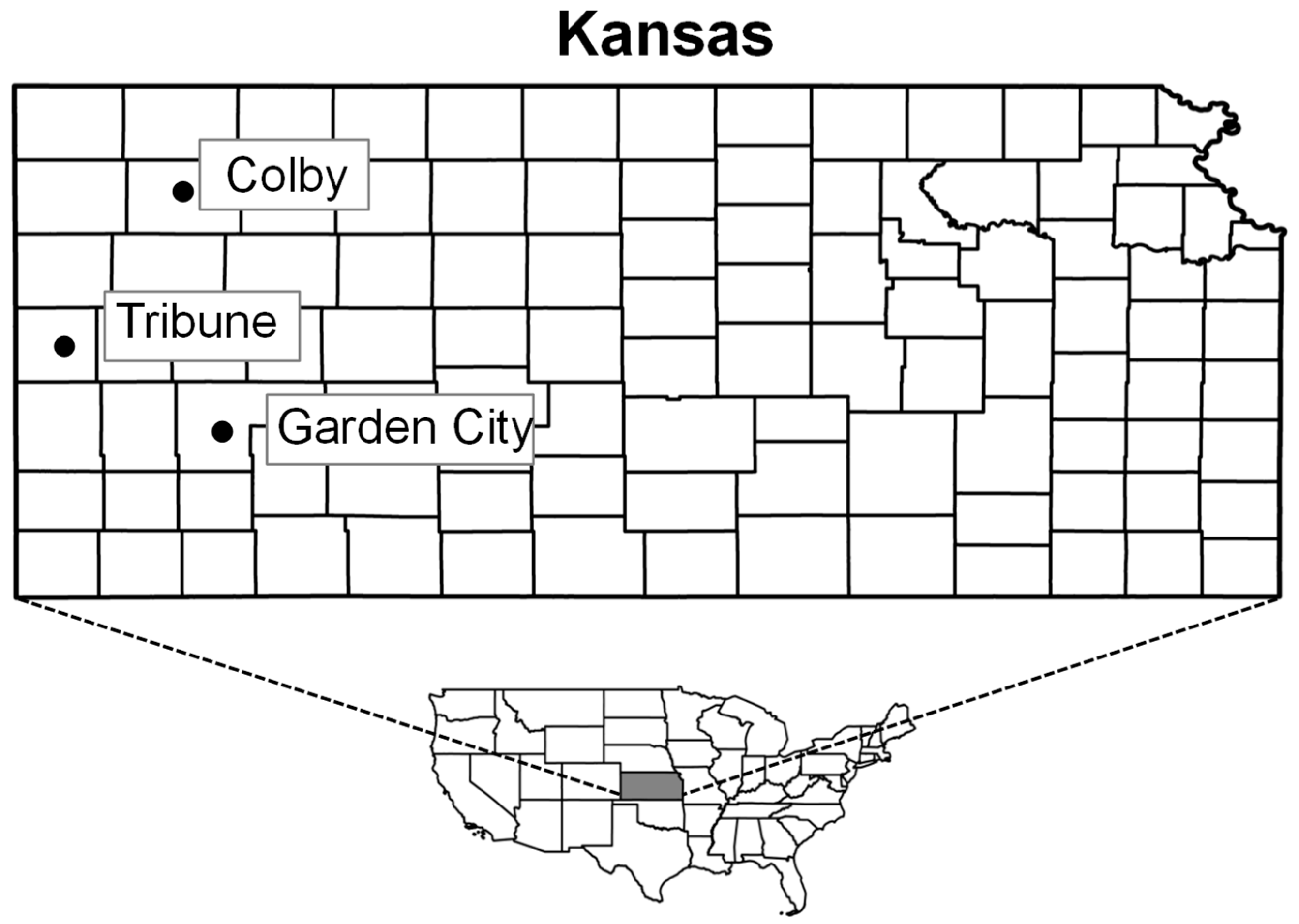
2.1. Cotton Growth Model and Site Characteristics

Because of its potential profitability, cotton growth and yield response to irrigation capacity and duration were modeled using the process-level cotton growth and yield simulation model GOSSYM ver. 4 [29]. GOSSYM required input parameters to describe daily weather, soil properties and conditions, agronomic management such as planting geometry or irrigation, elevation and geo-location, and cotton cultivar-specific factors governing growth and development in a variety file. Model uncertainty for plant height, leaf area index, and simulated water use was previously validated under semiarid conditions that showed calculated ET values were within 10% of measured use [30]. The model lint yield uncertainty under both dryland and irrigated conditions was validated for the Texas High Plains and in southwest Kansas, which indicated agreement between limited observed and modeled trials [10,31]. The 2006 to 2012 mean lint yields of multiple cultivars grown southwest of Garden City, near Hugoton, were regressed on the GOSSYM modeled cotton lint yield of one common variety file with good agreement, R² = 0.93, [10]. Observed higher, 1600–1800 kg ha⁻¹, yield levels were underestimated 10–20% by GOSSYM, possibly because the specified N fertility level was insufficient above 1200 kg ha⁻¹. Cotton growth and yield response to irrigation management as modified by climate for each ENSO phase was modeled for southwest Kansas at Garden City (37°58′ N, 100°51′ W; 865 m ASL), west-central Kansas at Tribune (38°28′ N, 101°45′ W; 1100 m ASL) and northwest Kansas at Colby (39°23′ N, 101°2′ W; 962 m ASL) (Figure 1).

Daily weather input parameters of solar irradiance (MJ m⁻²), maximum and minimum air temperature (°C), Ta, precipitation (mm), and wind run (km d⁻¹) required by the model were from long-term (1961–2000) weather records for each location. We confined simulations to the years 1961–2000 to avoid time series bias in weather input due to climate change as declared by IPCC [32], which insured random climate variability, i.e., a stationary time series [33], and no biased inferences for ENSO phase and irrigation effects. The 1961–2020 annual mean Ta for southwest Kansas, [34] with a best-fit line (dashed) in Figure 2 reveals a 0.16 °C decadal increase that would require detrending to remove bias. Compared with the 60-year Ta average of 12.8 °C (solid line), the 1961–2000 mean annual Ta was 12.6 °C with a decadal increase of 0.04 °C (red dotted line) or ¼ of the 1961–2020 trend, while the 2000–2020 mean annual Ta averaged 13.3 °C with no decadal trend (blue dotted line). The 0.7 °C step increase in Ta for years after 2000 causes the series climate data and, potentially, the dependent simulations to be non-stationary as required for unbiased inferences on treatment effects.

A 1.88-m deep Ulysses silt loam (Fine-silty, mixed, superactive, mesic Torriorthentic Haplustoll) was selected, and the required soil parameters used because it occurs in all three locations evaluated occupying county areas of at least 11% and increasing to 25%, but was not the dominant soil for any county [35,36,37]. The nearly level (~1.0% slope) Ulysses soil profile was divided into two layers that included a mollic epipedon (0.0–0.38 m) over a cambic horizon (0.38–1.88 m) above parent material with common bulk density, texture, and hydrologic properties adapted from pedon ID 89P0734 [38]. For all simulations, the soil profile had uniform initial plant available water content of 50% (~182 mm) that approximates the 197 mm available soil water at planting for deficit irrigated (127 mm application) corn, sorghum, or soybean in western Kansas [12]. Runoff of rain or irrigation in simulations was not permitted because the typical infiltration capacity into Ulysses soil is sufficient to produce negligible runoff [39]. Maximum modeled rooting depth was unrestricted within the 1.88 m Ulysses soil profile and was consistent with reported water extraction patterns for cotton grown in lysimeters with Ulysses soil at Bushland [40]. The typical Ulysses soil profile nitrogen of ~33 kg ha⁻¹ [38] was supplemented with 110 kg N ha⁻¹ to provide sufficient N to optimize crop water use for up to 700 mm [41] and potential lint yield of 1200 kg ha⁻¹ for growing seasons with desirable thermal energy [42]. When nutrients are deficient, the effect of fertilizer supplements on cotton performance would be expected but is unknown in Kansas. GOSSYM does not simulate the effects of nutrient deficiencies except for N on cotton growth, which would be near ideal.

2.2. ENSO Phase Classification

The ENSO phase was assigned for each year of simulation using the Niño 3.4 region (5° N–5° S, 120°–170° W) Oceanic Niño Index or ONI published by the National Weather Service Climate Prediction Center in monthly [43]. The ONI classifies ENSO phases based on a 3-month average deviation in observed equatorial sea surface temperatures from the corresponding 30-year reference temperature that is updated every 5 years to avoid climate change bias. The warm El Niño phase occurs when ONI exceeds 0.5 °C, and the cold La Niña phases have ONI values less than −0.5 °C while all exceptions to those conditions are ENSO phase Neutral. For each crop year, the ENSO phase was a same-year hindcast classification [44] based on the September through November (SON) ONI 3-month period that captures atmospheric coupling to sea surface temperature [45] of a maturing ENSO condition. Using the SON period ONI, we identified the ENSO phase for each year between 1961 and 2000 that comprised 13 years each for the El Niño and La Niña phases plus 14 years of Neutral phase conditions [46].

2.3. Simulations

Cotton growth, lint yield, and water use were simulated for dryland (precipitation only) and scenario deficit irrigation capacity and period duration using GOSSYM, currently available from USDA-ARS [47]. The modeled planting observed the regionally typical 0.76-m row spacing and 13 plants m⁻² population of a stripper type cultivar with an indeterminate growth habit similar to All-Tex Atlas (Levelland, TX, USA) as described in the variety file ST1 supplied with GOSSYM [30]. Simulations began two weeks before the designated DOY 145 emergence that followed 10 days after a 15 May target planting date. The growing season continued until plants reached physiological maturity (100% open bolls) or until the first freeze when lint yield and cumulative growing season ET were determined. Simulated crop growth parameters included, e.g., the number of open or green bolls at “first freeze” and leaf area index (LAI) captured at the first open boll.

Irrigations were applied every 7 days beginning 37 days after emergence or about the first square, i.e., flower bud initiation, which produced the earliest lint yield response to irrigation in the Texas South Plains [48]. Trial irrigation scenario periods were for 4, 6, or 8 weeks at rates of 2.5, 3.75, and 5.0 mm d⁻¹ or pumping capacities of ~0.29, 0.43, and 0.58 L s⁻¹ ha⁻¹ that represent regionally common weak, declining, or strong producing wells [49]. The combined effects of irrigation rate and duration produced a range of cumulative seasonal irrigation depths from 70 mm (4 weeks × 7 d/weeks × 2.5 mm/d) to 280 mm (8 weeks × 7 d/weeks × 5 mm/d), as shown in Figure 3. In summary, cotton growth and yield were simulated at three western Kansas sites for 10 irrigation scenarios that included all combinations of irrigation capacity (3 levels) and period (3 levels) plus dryland, 0.0 mm d⁻¹ evaluated during each of 40 years divided into three ENSO phases. Irrigation applications did not consider soil water storage capacity or precipitation because of the large profile potential storage capacity, ~180 mm, and low application rates with deficit irrigation.

2.4. Analyses

Cotton growth, lint yield (Y_L) in kg ha⁻¹, seasonal crop water use or ET (m³ ha⁻¹), and crop water productivity (CWP) calculated according to Zwart and Bastiaanssen [50] from the equation:

$$\mathrm{CWP}=\frac{{\mathrm{Y}}_{\mathrm{L}}}{\mathrm{ET}} (\mathrm{kg}·{\mathrm{m}}^{-3})$$

(1)

were compared in response to irrigation scenario and ENSO phase at each location. The growing seasons (1961–2000) provide normal climatic variability, e.g., rainfall and temperature, for the identified ENSO phase, as well as random experimental variability for comparing GOSSYM-modeled cotton performance. Annual climate variability affecting cotton growth and yield was parameterized in terms of cumulative CGDD from a calculated daily average of the maximum and minimum Ta minus the 15.6 °C base according to method 1 of McMaster and Wilhelm [51]. The ENSO phase-specific CGDD, precipitation, and lint yields were plotted by declining rank for the combined irrigation scenarios at each location as a function of the untransformed exceedance probability [52]. Simulated cotton growth, lint yield, and water use response to the ENSO phase and the scenario irrigation capacity and duration fixed effects together with observation years random effects were compared by a factorial arrangement of a completely randomized design using a SAS ver. 9.4 mixed model ANOVA [53]. As some exceedance probability plots appeared to show possible differences among these data series, a Wilcoxon nonparametric analysis with a Conover test was modeled by the SAS NPAR1WAY to corroborate ANOVA inferences. Locations were analyzed independently for better control of heteroscedastic variability. Unless otherwise specified, all statistical analysis effects were declared significant at the 0.05 probability level.

3. Results and Discussion

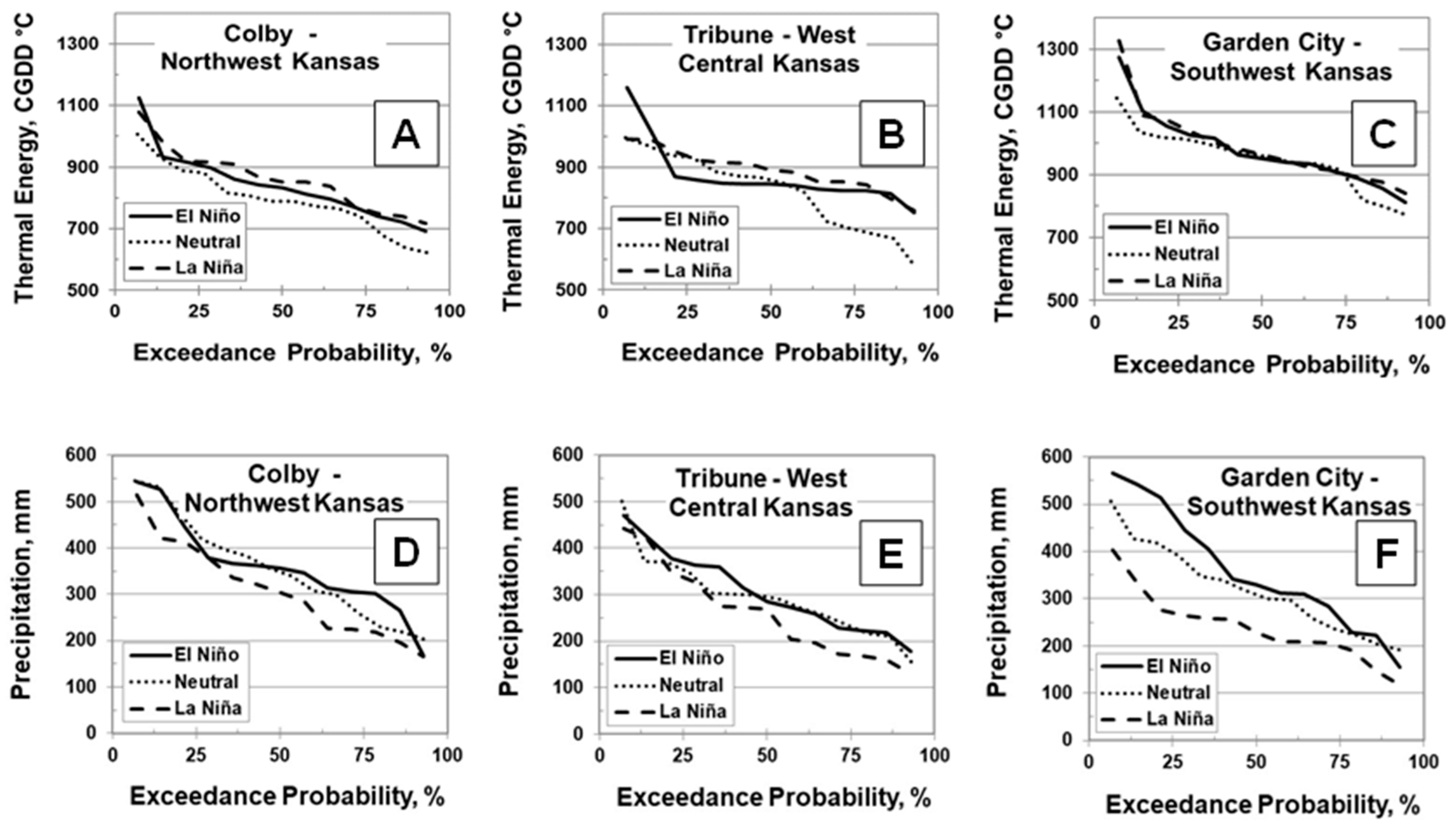
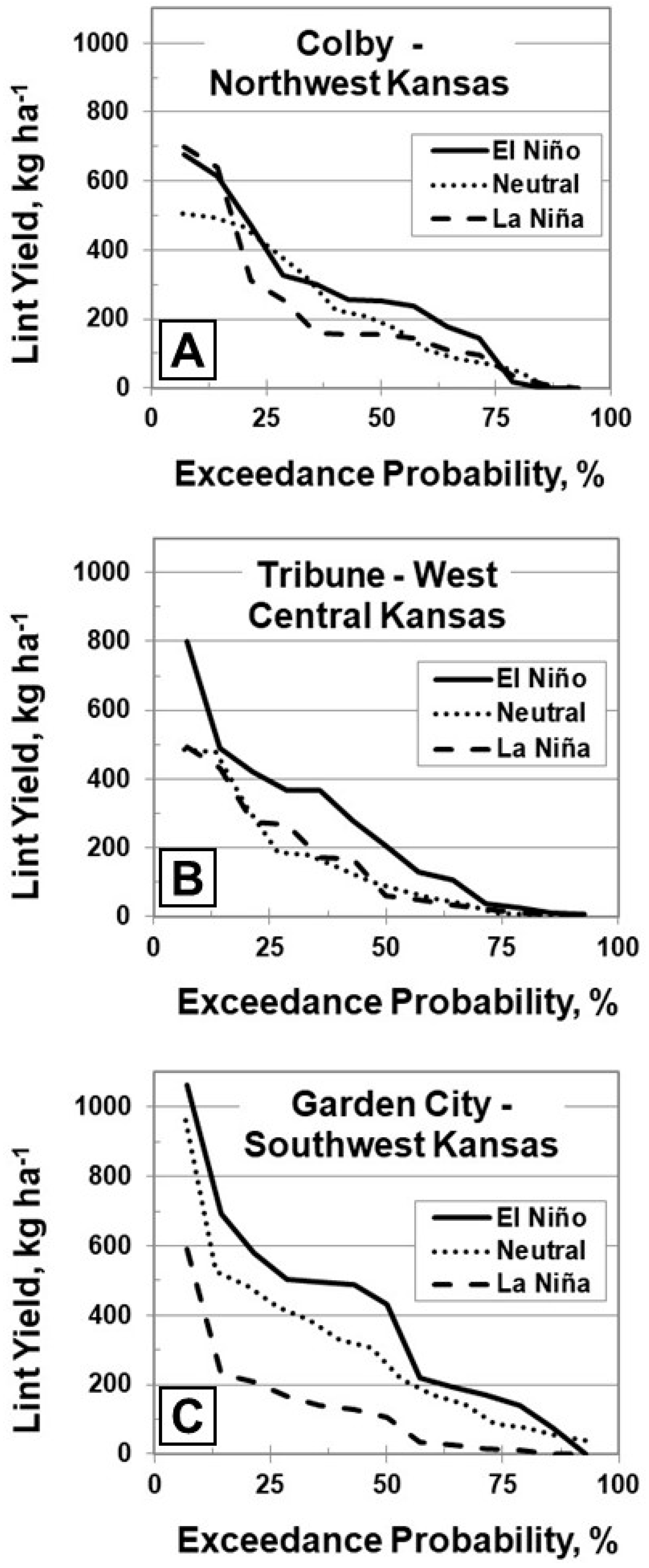
3.1. ENSO Phase Effects on Thermal Energy, Precipitation, and Lint Yield

The effect of the ENSO phase on Western Kansas climate was characterized by subsequent evaluation of potential cotton growth and yield response for various irrigation capacity and period scenarios. Annual variability of growing season energy and precipitation are plotted as a function of exceedance probability at Colby, Tribune, and Garden City for all ENSO phases (Figure 4A–F). The CGDD that generally governs cotton growth, fruit formation, and yield [54] averaged similar 832 CGDD°C at Colby in northwest Kansas and 860 CGDD°C at Tribune in west-central Kansas but increased significantly to 973 CGDD°C at Garden City in southwest Kansas. Thermal energy for Colby ranged from a high of 1124 CGDD°C down to 630 CGDD°C minimum (Figure 4A) with no significant (p > 0.36) differences among the ENSO phases that averaged 841 CGDD°C for El Niño, 795 CGDD°C for Neutral, and 867 CGDD°C for La Niña. The CGDD for west-central Kansas (Figure 4B) similarly ranged from a high 1159 to 573 CGDD°C, and the ENSO phase means 871 CGDD°C for El Niño, 820 CGDD°C for Neutral, and 889 CGDD°C for La Niña. No significant (p > 0.21) differences in CGDD among ENSO phases were identified using ANOVA, which was corroborated (p = 0.42) by Wilcoxon nonparametric methods. Further analysis of the noticeably lower thermal energy during Neutral compared with La Niña and El Niño phase years at exceedance p levels > 70% were significant (p = 0.03) according to the data dispersion sensitive Conover test. We, however, offer no explanation for it appearing only during the Neutral phase years. Southwest Kansas maximum CGDD (Figure 4C) ranged from 1144 for Neutral to 1327 CGDD°C for La Niña phase years with corresponding lows of 771 and 840 CGDD°C and seasonal means of 949 and 990 CGDD°C that did not differ (p > 0.64) from each other or the intervening 980 CGDD°C for El Niño. The expected greater temperatures and related increased thermal energy during drier years of La Niña with historically warmer air temperatures compared with Neutral or El Niño years [13,14] were not observed.

Western Kansas precipitation averaged 311 ± 27.5 mm during the 1961–2000 growing season, but the 341 mm precipitation for northwest Kansas at Colby was significantly greater than the 287 mm mean precipitation at Tribune, and 305 mm mean at Garden City. The ENSO phase mean precipitation of 360 mm for El Niño years, 355 mm for Neutral years, and the numerically lower but not significantly different 308 mm average for La Niña phase years. Nevertheless, 70% of the precipitation observations during the La Niña phase years at Colby were lower than the median precipitation values for the El Niño and Neutral (Figure 4D) phases. Seasonal precipitation for west-central Kansas at Tribune (Figure 4E) averaged 287 mm and included ENSO phase means of 306 mm for El Niño, 295 mm for neutral, and 260 mm for La Niña that did not differ (p > 0.42). The observed median precipitation during El Niño or Neutral phase years at Tribune, however, exceeded precipitation during La Niña phase years with exceedance probabilities > 30%. Precipitation for southwest Kansas at Garden City averaged 305 mm overall, ranging from a low precipitation mean of 238 mm for the La Niña phase years up to the significantly (p = 0.04) larger 319 mm and 358 mm totals for Neutral and El Niño phase years (Figure 4F). During the 1961–2000 test period, precipitation for northwest and west-central Kansas exhibited no differences due to the ENSO phase. Southwest Kansas exhibited more pronounced ENSO effects manifested as drier La Niña phase and wetter El Niño phase weather patterns.

Simulated dryland lint yields are plotted as a function of exceedance probability at each western Kansas location for all ENSO phases in Figure 5. Overall, the western Kansas 40-year dryland yield averaged 230 kg ha⁻¹ with site means that ranged from 272 kg ha⁻¹ at Garden City in southwest Kansas to 183 kg ha⁻¹ at Tribune in west-central Kansas and 235 kg ha⁻¹ at Colby in northwest Kansas. The lower yields at Tribune and Colby were attributed to decreased seasonal CGDD with increasing elevation and latitude, as previously reported [9,10]. During the El Niño phase years, the dryland lint yield across all western Kansas locations averaged 302 kg ha⁻¹ or 31% more than the overall yield due to 30 mm more precipitation (341 mm). By contrast, seasonal precipitation during drier La Niña years averaged 269 mm across western Kansas with a mean simulated dryland yield of 165 kg ha⁻¹ for a 28% yield reduction. In northwest Kansas, the simulated lint yields of 268 kg ha⁻¹ for El Niño and 222 kg ha⁻¹ for Neutral phase years were not significantly different (p = 0.78) from the 20% smaller mean lint yield of 214 kg ha⁻¹ during La Niña phase years. Nevertheless, the simulated lint yields for El Niño and Neutral phase years were not always greater than for La Niña (Figure 5A). For west-central Kansas at Tribune, the overall mean dryland yield of 183 kg ha⁻¹ used like mean yields of 152 kg ha⁻¹ for Neutral and 148 kg ha⁻¹ for La Niña phase years (Figure 5B) and the 66% larger but not significantly different 249 kg ha⁻¹ yield for El Niño phase years. These yields appear incongruent with the corresponding growing season precipitation of 295 mm and 306 mm for Neutral and El Niño phase years (respectively) that decreased to 260 mm for La Niña years. The impact of the ENSO phase on yield in southwest Kansas (Figure 5C) was attributed to precipitation amounts (Figure 4D–F) that, compared with La Niña phase years, increased by 120 mm for El Niño and 81 mm for Neutral phase years. The resulting simulated dryland yield for Garden City in southwestern Kansas averaged 389 kg ha⁻¹ for El Niño compared with the not significantly lower (p = 0.07) Neutral phase yield of 300 kg ha⁻¹ and the significantly lower (p = 0.03) 128 kg ha⁻¹ La Niña phase yield (Figure 5C). These ENSO phase hindcast yield responses show the observed precipitation amounts that may support climate-informed management of crop irrigation to improve yield and water productivity as described for the southern Great Plains [55].

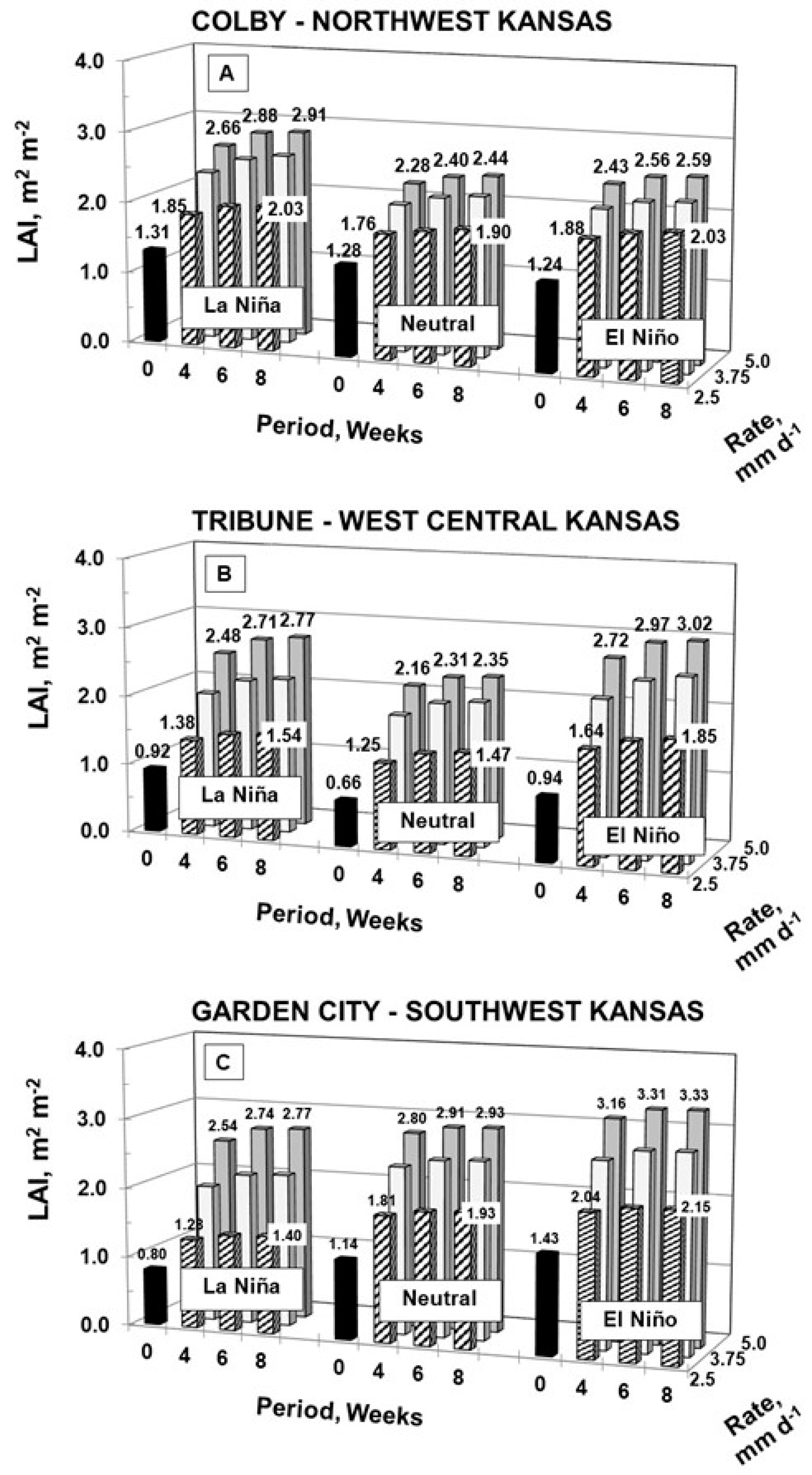
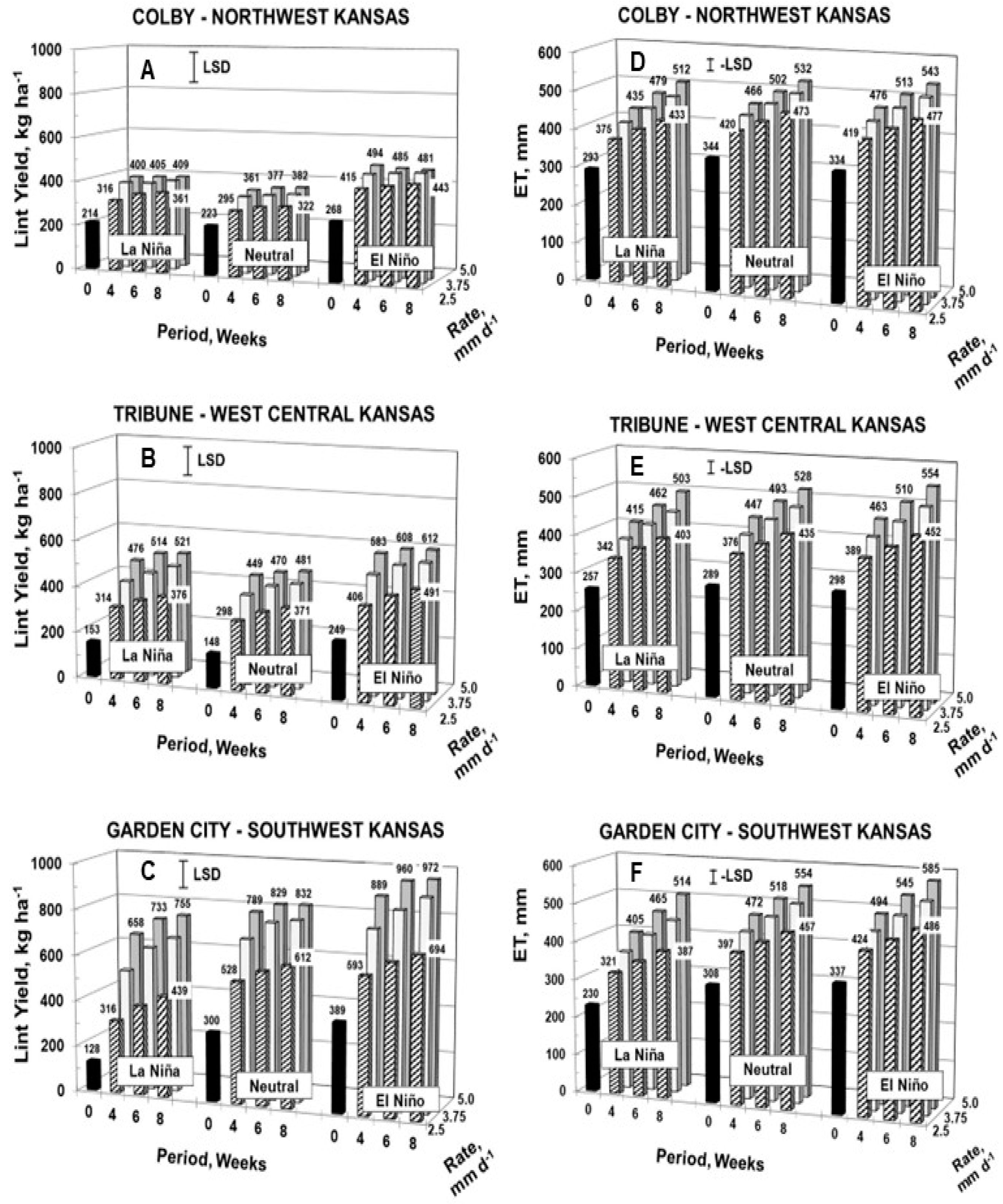
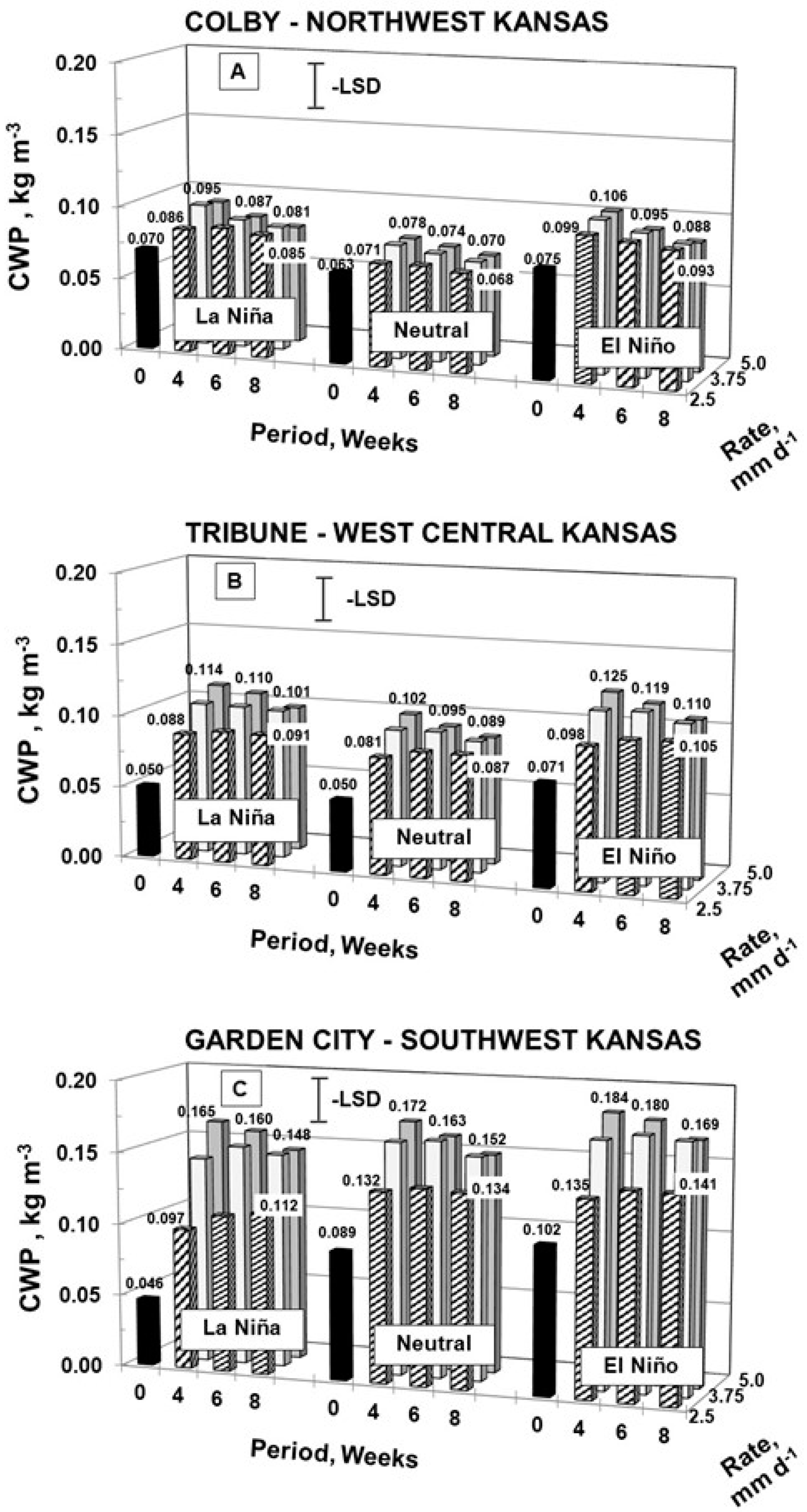
3.2. Crop Response to ENSO Phase and Scenario Irrigation Capacity and Duration Effects

Location-specific mean 1961–2000 simulated leaf area index (LAI) and the boll number at first open boll and the later fraction of open bolls at freeze are reported with the ANOVA results for ENSO phase and scenario irrigation capacity and duration fixed effects by site in

Table 1. Location-specific mean 1961–2000 simulated cotton leaf area index (LAI) at 1st open boll, final boll number, and the fraction of bolls that were open with the corresponding ANOVA significance levels for ENSO Phase (P) and scenario irrigation Capacity (C), and Period (D) fixed effects.

		LAI at 1st Open Boll			Boll Number at 1st Open Boll			Fraction of Bolls Opened
EFFECT †		Colby	Tribune	Garden City	Colby	Tribune	Garden City	Colby	Tribune	Garden City
ENSO Phase		m2 m−2			bolls m−2			%
El Niño		2.26 a †	2.38 a	2.72 a	37.5 a	42.4 a	48.6 a	47.2 a	53.8 a	74.5 a
Neutral		2.13 a	1.88 a	2.42 ab	35.7 a	37.0 a	46.0 a	33.4 a	41.6 a	64.4 a
La Niña		2.44 a	2.09 a	2.04 b	42.4 a	40.6 a	41.9 a	33.4 a	44.4 a	65.3 a
Irrigation Capacity, mm d−1
2.5		1.92 c	1.54 c	1.78 c	35.5 b	33.9 c	36.7 c	41.0 a	53.0 a	74.4 a
3.75		2.33 b	2.19 b	2.46 b	39.7 a	41.4 b	47.9 b	36.9 b	44.7 b	65.9 b
5.0		2.57 a	2.61 a	2.94 a	40.5 a	44.8 a	52.0 a	36.1 b	42.1 b	63.9 b
Irrigation Period, weeks
4		2.16 b	1.96 b	2.29 b	38.2 a	38.5 b	43.9 b	39.0 a	49.0 a	70.4 a
6		2.30 a	2.16 a	2.43 a	38.7 a	40.5 a	46.2 a	37.6 b	46.1 b	67.5 b
8		2.35 a	2.22 a	2.45 a	38.7 a	41.1 a	46.4 a	37.5 b	44.8 b	66.4 b
ENSO Phase × Irrigation Capacity
El Niño	×2.5	1.97 cd	1.76 de	2.11 cde	34.7 ab	36.0 bc	39.8bcd	51.3 a	61.8 a	80.8 a
El Niño	×3.75	2.28 bcd	2.46 bc	2.77 ab	37.8 ab	44.1 abc	51.1 abc	46.8 ab	51.1 ab	71.5 bc
El Niño	×5.0	2.53 ab	2.91 a	3.27 a	39.8 ab	47.3 a	54.9 a	43.6 abc	48.6 ab	71.1 bc
Neutral	×2.5	1.83 d	1.38 e	1.88 ef	32.3 b	31.8 c	38.0 cd	35.8 bc	47.4 b	69.9 bc
Neutral	×3.75	2.17 bcd	1.98 cd	2.50 bcd	36.7 ab	38.3 abc	48.3 abc	32.7 c	39.8 b	62.7 cd
Neutral	×5.0	2.37 abc	2.28 bc	2.88 a	38.1 ab	40.8 abc	51.9 ab	31.7 c	37.6 b	60.6 cd
La Niña	×2.5	1.96 cd	1.47 e	1.35 f	39.3 ab	34.0 c	32.2 d	35.9 bc	49.9 ab	72.5 ab
La Niña	×3.75	2.53 ab	2.14 cd	2.10 de	44.6 a	41.7 abc	44.4 abc	31.2 c	43.4 b	63.6 bcd
La Niña	×5.0	2.82 a	2.65 ab	2.68 abc	43.4 a	46.2 ab	49.2 abc	33.0 c	40.1 b	60.0 cd
EFFECT		P > F			P > F			P > F
ENSO Phase (P)		0.49	0.13	0.05	0.13	0.39	0.35	0.21	0.39	0.22
Irrigation Capacity (C)		<0.01	<0.01	<0.01	<0.01	<0.01	<0.01	<0.01	<0.01	<0.01
P × C		<0.01	<0.01	0.01	0.14	0.40	0.73	0.01	0.40	0.53
Irrigation Period (D)		<0.01	<0.01	<0.01	0.52	0.01	0.01	0.05	<0.01	<0.01
D × P		0.73	0.91	0.96	0.98	0.74	0.96	0.72	0.90	0.96
D × C		0.95	0.67	0.91	0.43	0.89	0.16	0.40	0.94	0.25
D × C × P		>0.99	0.99	>0.99	0.77	>0.99	0.91	0.95	>0.99	0.98

^† Effect means within columns followed by the same letter are not significantly different, p = 0.05.

. Simulated cotton LAI averaged 2.39 m² m⁻² in southwest Kansas at Garden City compared with the significantly smaller LAI means of 2.27 and 2.11 m² m⁻² at Colby and Tribune. The LAI decreased significantly with incrementally decreasing irrigation capacity at all locations (Figure 6A–C) because reduced water availability depressed plant growth and, as a result, the LAI. Continued canopy growth during extended irrigation periods resulted in significantly smaller LAI for the 4-week irrigation duration compared with 6- and 8-week durations for all three locations (Table 1). The significant phase by irrigation capacity interaction revealed no consistent trend on LAI along either fixed effect array and may be a further expression of irrigation capacity effects. Greater precipitation during the El Niño phase at Garden City, however, appeared to diminish irrigation capacity effects compared with La Niña. At Garden City, the increased precipitation during the El Niño phase increased LAI significantly over LAI during the drier La Niña phase (Figure 6C). When water availability is not limited, cotton directs assimilate to boll development and canopy expansion that increases these parameters as described over decades [56,57]. Our simulations show the LAI of an expanding cotton canopy increased with both increasing application capacities and durations over 4 weeks because irrigation better meets crop water demand; that is, the available water was sufficient to supply crop ET.

The simulated boll number at first freeze (Table 1) averaged 38.5- and 40.0- bolls m⁻² for Tribune and Colby Kansas, which was significantly fewer than the more numerous 45.5 bolls m⁻² at Garden City. Boll number was invariant among ENSO phases at any location, including Garden City, despite significantly greater precipitation during El Niño compared with La Niña phases, in contrast to the significant LAI differences at Garden City. At all locations, the boll number increased significantly as irrigation capacity exceeded 2.5 mm d⁻¹ and, again, after capacity exceeded 3.75 mm d⁻¹ at Tribune because of its lower precipitation and at Garden City, where CGDD extended cotton growth and water use. Boll number also increased significantly when irrigation durations exceeded 4 weeks at Tribune and Garden City, but the limited CGDD at Colby diminished boll number response to irrigation and precipitation [10]. Results show early growth and fruiting increased with increasing irrigation plus precipitation; that is, LAI and boll number increased at Garden City as precipitation increased during El Niño or as scenario irrigation capacity or period increased.

Cotton yield varies with both the total boll number and the fraction of those bolls that mature open for harvest. The simulated mean fraction of open bolls at first freeze ranged from 68% in southwest Kansas at Garden City to significantly lower values of 38% at Tribune and 47% at Colby in west-central and northwest Kansas. Although not differing significantly by ENSO phase, the fraction of open bolls during El Niño years was from 10% to 16% greater than for the similar Neutral or La Niña ENSO phases (Table 1). In contrast to either the simulated LAI or boll number, the fraction of open bolls improved significantly with reduced water applications, i.e., more bolls opened for the 2.5 mm d⁻¹ scenario irrigation capacity and 4-week period duration than for larger irrigation capacities or durations. The lower capacity and shorter duration scenario irrigation reduced fruiting and canopy expansion, but the reduced assimilate production was directed in priority to maturing harvestable bolls rather than producing green bolls, as suggested by Pabuayon et al. [57]. Also, longer scenario irrigation periods may delay maturation sufficiently for a limited CGDD growing season to reduce the fraction of open bolls and limit yield.

Mean simulated cotton lint yields are listed by location for each ENSO phase and scenario irrigation capacity and period duration in addition to their combinations with the corresponding ANOVA in

Table 2. Location-specific mean 1961–2000 simulated cotton lint yield, water use, and crop water productivity with the corresponding ANOVA significance levels for ENSO Phase (P) and scenario irrigation Capacity (C) and Period (D) fixed effects.

		Lint Yield			Crop Water Use—ET			Crop Water Productivity
EFFECT †		Colby	Tribune	Garden City	Colby	Tribune	Garden City	Colby	Tribune	Garden City
ENSO Phase		kg ha−1			mm			kg m−3
El Niño		463 a †	534 a	811 a	482 a	467 a	500 a	0.097 a	0.112 a	0.163 a
Neutral		346 a	409 a	712 ab	475 a	450 a	474 a	0.073 a	0.091 a	0.152 a
La Niña		380 a	432 a	567 b	442 a	418 a	409 b	0.088 a	0.101 a	0.137 a
Irrigation Capacity, mm d−1
2.5		361 b	379 c	534 c	433 c	400 c	412 c	0.084 b	0.092 b	0.126 b
3.75		407 a	473 b	732 b	471 b	449 b	464 b	0.088 a	0.105 a	0.160 a
5.0		421 a	524 a	824 a	495 a	486 a	506 a	0.086 ab	0.107 a	0.166 a
Irrigation Period, weeks
4		386 a	425 b	639 c	433 c	406 c	419 c	0.091 a	0.103 a	0.151 a
6		398 a	465 a	710 b	468 b	446 b	463 b	0.086 b	0.103 a	0.153 a
8		405 a	485 a	741 a	498 a	482 a	500 a	0.081 c	0.099 a	0.148 a
Irrigation Capacity by Period
2.5	×4	342 d	339 f	479 f	405 f	369 g	380 h	0.085 bc	0.089 e	0.121 d
2.5	×6	365 cd	384 e	542 e	434 e	400 f	413 g	0.085 bc	0.094 de	0.129 d
2.5	×8	375 bc	413 de	582 e	461 d	430 e	443 e	0.082cd	0.094 de	0.129 d
3.75	×4	399 ab	435 d	658 d	436 e	408 f	421 f	0.094 a	0.106 bc	0.158 bc
3.75	×6	406 a	481 c	749 c	473 c	451 c	466 c	0.087 b	0.106 bc	0.163 abc
3.75	×8	416 a	504 abc	790 bc	505 b	488 b	506 b	0.083 cd	0.102 bc	0.158 bc
5.0	×4	418 a	502 bc	779 c	459 d	442 d	457 d	0.093 a	0.114 a	0.174 a
5.0	×6	422 a	531 ab	840 ab	498 b	488 b	509 b	0.085 bc	0.108 ab	0.168 ab
5.0	×8	424 a	538 a	853 a	529 a	528 a	551 a	0.080 d	0.100 cd	0.156 c
EFFECT		P > F			P > F			P > F
ENSO Phase (P)		0.49	0.41	0.02	0.23	0.15	<0.01	0.54	0.59	0.42
Irrigation Capacity (C)		<0.01	<0.01	<0.01	<0.01	<0.01	<0.01	0.05	<0.01	<0.01
P × C		0.99	0.84	0.23	0.09	0.92	<0.01	0.81	0.65	0.06
Irrigation Period (D)		0.08	<0.01	<0.01	<0.01	<0.01	<0.01	<0.01	0.10	0.24
D × P		0.96	>0.99	0.74	0.64	0.82	0.09	0.60	>0.99	0.84
D × C		0.72	0.59	0.66	0.15	<0.01	<0.01	0.06	0.02	0.03
D × C × P		>0.99	>0.99	>0.99	>0.99	>0.99	0.95	0.99	>0.99	>0.99

^† Effect means within columns followed by the same letter are not significantly different, p = 0.05.

. Overall, simulated lint yields averaged 396 kg ha⁻¹ at Colby and 459 kg ha⁻¹ at Tribune compared with the significantly higher 697 kg ha⁻¹ lint yield at Garden City because the lower elevation and latitude favored the ~15% higher seasonal CGDD [9,10]. Greater simulated lint yields for sites with decreasing latitude and elevation, in addition to a pronounced ENSO effect in southwest Kansas, were observed (Figure 7A–C). While Colby and Tribune yields were numerically lowest for the neutral phase, those simulated lint yields for northwest and west-central Kansas did not differ significantly from the ENSO phase (Table 2). In southwest Kansas at Garden City, however, the lint yield of 811 kg ha⁻¹ for El Niño was significantly greater than the 567 kg ha⁻¹ yield for La Niña phase years (Table 2). Because mean growing season energy did not differ among ENSO phases at Garden City, the 30% lower lint yield for La Niña was attributed to the 120 mm reduction in growing season precipitation for La Niña compared with El Niño phase years. This significant yield difference mirrors the ENSO phase effects on precipitation (Figure 4D–F) and supports ENSO phase-dependent climate-informed management.

Crop response to greater CGDD and water availability was manifested as increasing lint yields following a gradient from higher to lower site latitudes and elevations combined with both ENSO phase and scenario irrigation capacity or duration effects (Figure 7A–C). At Colby, for example, increasing the irrigation capacity from 2.5 mm d⁻¹ to 3.75 or 5.0 mm d⁻¹ increased mean lint yield by 15% from 361 kg ha⁻¹ to a not statistically different 407 and 421 kg ha⁻¹ yield. Increasing irrigation periods from 4 to 8 weeks yielded lint totals that differed by < 20 kg ha⁻¹ or ~5% overall (Table 2). With the higher CGDD at Garden City, the overall average dryland yield of 272 kg ha⁻¹ nearly doubled to 534 kg ha⁻¹ when irrigated at the 2.5 mm d⁻¹ capacity, then further improved by 37% or 54% with 3.75 or 5.0 mm d⁻¹ capacities. Increasing the irrigation period from 4 up to 6 or 8 weeks also improved yields because of increased applied water. Likewise, simulated lint yields at Tribune increased significantly as scenario irrigation capacity increased and for durations exceeding 4 weeks.

The overall location mean simulated cotton ET ranged from a low of 445 mm at Tribune to significantly larger 461 mm and 467 mm ET observations at Garden City ET and Colby, Kansas (Table 2). No significant differences in ENSO phase-dependent ET were identified except for southwest Kansas, where reduced ET at Garden City during the drier La Niña phase was 75% to 80% of the seasonal precipitation differences for El Niño and Neutral phases (Figure 4D,E). That is, southwest Kansas received from 80 to 120 mm more precipitation during the Neutral and El Niño phases compared with the La Niña phase and probably contributed to the corresponding 65- and 91-mm increase in ET over the 409 mm ET observed for La Niña phase years. Also exclusive to southwest Kansas, a significant ENSO phase interaction with irrigation capacity revealed a 25% broader ET range across scenario capacities during the drier La Niña than for the El Niño or Neutral phases (Figure 7F) that we attribute to water deficit stresses met by irrigation. This is shown for each location by incrementally higher simulated ET in Figure 7D–F as scenario irrigation capacities and period durations governing total water applications increased.

Mean CWP (Figure 8) calculated from simulated lint yield and ET of 0.086 kg m⁻³ in northwest Kansas at Colby increased modestly to 0.101 kg m⁻³ in west-central Kansas at Tribune. The 50–75% larger CWP (p = 0.05) for southwest Kansas at Garden City of 0.151 kg m⁻³ (Table 2) reflects the impact of greater growing season energy increase. The CWP did not differ with the ENSO phase at any location, including Garden City, despite having 120 mm more rain and 30% higher lint yields for El Niño than the significantly smaller yield for La Niña phase years with a corresponding 20% reduction in ET. Consistent with yields, the CWP for the 2.5 mm d⁻¹ scenario irrigation capacity was significantly lower than for 3.75- or 5.0-mm d⁻¹ irrigation capacities that typically promote an earlier maturing crop. The equivalent CWP values listed for 2.5- and 5.0-mm d⁻¹ capacity irrigation at Colby probably reflect yield limitations under the prevailing growing season energy that may also explain why increasing scenario irrigation period reduced CWP significantly at Colby. The significant interacting scenario irrigation capacity and period effects on CWP for Colby, Tribune, and Garden City declined with increasing irrigation duration for the 5 mm d⁻¹ capacity but reversed at Tribune and Garden City for the 2.5 mm d⁻¹ capacity (Figure 8). We conclude that climate-informed irrigation management in Western Kansas must balance irrigation capacity and period duration application levels with crop demand as governed by the available CGDD to optimize CWP and lint yield.

3.3. Split Center-Pivot Irrigation and Water Conservation

Modeled yield response in western Kansas can be summarized as showing greater irrigation capacity and period length increased both applied water and yield, but the location CGDD limited the effectiveness of increased applied water to improve yield at higher latitudes or elevations. Except at Garden City during La Niña, full pivot simulated lint yields at all locations for the 4-week 140 mm irrigation exceeded or did not differ (p = 0.95) from yields for the 8-week irrigations (140 to 280 mm) during both La Niña and El Niño phases (

Table 3. Mean 1961–2000 simulated cotton lint yield during La Niña and El Niño years at Colby—Northwest Kansas, Tribune—West Central Kansas, and Garden City—Southwest Kansas for dryland (D) and uniform irrigation (I) at capacities of 2.5, 3.75, 5.0 mm d⁻¹. The uniform 2.5 mm d⁻¹ “Full” irrigation totaled 70 mm over 4 weeks and 140 mm over 8 weeks, as a basis, was compared with weighted-average yield for irrigated (I) to dryland (D) pivot split combinations I:D of 2:1 and 1:1.

			La Niña					El Niño
Irrigation			Full Pivot		Split Pivot Application Depth, mm			Full Pivot		Split Pivot Application Depth, mm
Capacity, mm d−1	Depth, mm, at		4- weeks	8- weeks		70	140	4- weeks	8- weeks		70	140
	4- weeks	8- weeks	Lint Yield, kg ha−1		I:D Split	Lint Yield, kg ha−1 (Base Fraction)		Lint Yield, kg ha−1		I:D Split	Lint Yield, kg ha−1 (Base Fraction)
Colby
Dryland	0	0	214	214				268	268
2.5	70	140	316 b †	361ab	F	316 (88%)	361 (100%)	415 c	443 bc	F	415 (94%)	443 (100%)
3.75	105	210	386 a	404 a	2:1	329 (91%)	341 (94%)	466 ab	480 a	2:1	400 (90%)	409 (92%)
5.0	140	280	400 a	409 a	1:1	307 (85%)	311 (86%)	494 a	481 a	1:1	381 (86%)	374 (85%)
					Across ENSO Phase LSD = 213 kg ha−1
Tribune
Dryland	0	0	153	153				249	249
2.5	70	140	314 c	376 bc	F	314 (83%)	376 (100%)	406 c	491 b	F	406 (82%)	491 (100%)
3.75	105	210	404 b	485 a	2:1	320 (85%)	375 (100%)	514 b	579 a	2:1	426 (87%)	469 (95%)
5.0	140	280	476 a	521a	1:1	314 (84%)	337 (90%)	583 a	612 a	1:1	416 (85%)	431 (88%)
					Across ENSO Phase LSD = 195 kg ha−1
Garden City
Dryland	0	0	128	128				389	389
2.5	70	140	316 e	439 d	F	316 (72%)	439 (100%)	593 c	694 b	F	593 (85%)	694 (100%)
3.75	105	210	516 c	673 b	2:1	387 (88%)	492 (112%)	768 b	912 a	2:1	642 (92%)	738 (106%)
5.0	140	280	658 b	755 a	1:1	393 (90%)	441 (101%)	889 a	972 a	1:1	639 (92%)	680 (98%)
					Across ENSO Phase LSD = 191 kg ha−1

^† Application strategy (uniform or split pivot) yield means within the same ENSO phase and location followed by the same letter are not significantly different, p = 0.05.

), because high irrigation capacities better met early ET needs. Our simple Split center-pivot irrigation adds dryland production at a 2:1 and 1:1 irrigated to dryland spatial partition to an otherwise uniformly irrigated pivot to decrease groundwater withdrawals. An expected consequence is a lower area-averaged yield, but increasing the irrigation capacity has increased crop productivity and may restore some of the reduced yields of a uniformly irrigated pivot.

For fixed 70- and 140-mm application amounts, we also list the area-averaged yields of 2:1 and 1:1 split center-pivot irrigation for the corresponding capacities of 3.75 and 5.0 mm d⁻¹ at all sites and both ENSO phases in Table 3. The 8-week by 2.5 mm d⁻¹, 140 mm, full center-pivot deficit irrigation represents a water spreading strategy that relies on precipitation to meet crop water demand that we used as a basis for comparison with split center-pivot options. Compared with those reference yields, the 70- and 140-mm irrigation levels at Colby in northwest Kansas during both ENSO phases ranged from 90% to 94% for the 2:1 and ~85% for the 1:1 split center-pivot irrigation strategies. When applying half the base irrigation amount, using either split-pivot strategy at Colby preserved > 85% of the simulated lint yield of the uniformly irrigated full pivot at 2.5 mm d⁻¹ capacity. Similarly, the yields for 70mm split center-pivot irrigation strategies at Tribune in west-central Kansas were from 84% to 87% of the base irrigation regardless of the ENSO phase. By contrast, the 140-mm irrigation yield fractions of 100% for the 2:1 and 90% for a 1:1 center-pivot split during La Niña decreased slightly to 95% and 88% for El Niño phase years, showing split center-pivot irrigation at Tribune had no great yield advantage. At Garden City, the calculated 70 mm split center-pivot irrigation yields for 2:1 and 1:1 irrigation strategies preserved from 88% to 92% of the uniform 2.5 mm d⁻¹ 140 mm reference yield on half the irrigation amount independent of the ENSO phase. Using the 2:1 split center-pivot application strategy for the 140 mm irrigation increased yield above the base uniform full-pivot irrigation yields by 12% during La Niña years and 6% for El Niño years. Compared with the 140 mm uniform full-pivot irrigation base yield, the 1:1 split center-pivot irrigation strategy yields were practically no different for the La Niña and El Niño phase years. These results show any yield benefit using split center-pivot irrigation strategies to divert uniformly applied water from a dryland fraction to irrigate the remaining area at a greater capacity is more pronounced in southwest Kansas during drier La Niña phase years. Irrigation plus precipitation in southwest Kansas produced and matured less fruit during La Niña than during El Niño phase years because greater precipitation with El Niño promoted robust plant growth and more matured bolls.

4. Summary and Conclusions

No ENSO phase effect on CGDD was identified for western Kansas. That is, warmer summer temperatures typically associated with the La Niña phase [13] were absent at the western Kansas sites, indicating no relief from CGDD limitations may be expected or exploited during this phase. Seasonal precipitation did not vary with the ENSO phase in west-central and northwest Kansas, possibly due to a weak ENSO phase signal or an ENSO climate pattern reversal between southern and northern latitudes that transitions in central or northern Kansas, if not Nebraska [13]. In southwest Kansas, greater seasonal precipitation manifested during El Niño phase years was greater and decreased for La Niña years, resulting in similar yield differences. It was concluded that, as ENSO phase-based seasonal climate predictions improve, ENSO climate information may permit successful adjustment of dryland or irrigated land allocations or related fertility levels for optimum cotton production in southwest Kansas.

Simulated mean lint yield of ~700 kg ha⁻¹ across all irrigation levels and durations in southwest Kansas at Garden City was 33% larger than at Tribune (460 kg ha⁻¹) in west-central Kansas and 43% larger than at Colby (~400 kg ha⁻¹) in northwest Kansas due to greater CGDD as elevation and latitude increased [9,10]. Yields ranged from a low of 316 kg ha⁻¹ for the 2.5 mm d⁻¹ by 4-week irrigation during La Niña up to a ~300% higher yield of 972 kg ha⁻¹ for 5.0 mm d⁻¹ by 8-week irrigation during El Niño at Garden City. By contrast to the yield range of 656 kg ha⁻¹ at Garden City, yield differences at Tribune decreased 52% to 314 kg ha⁻¹ and 70% to 199 kg ha⁻¹ at Colby because the CWP, like yield, depends on seasonal CGDD. Simulated lint yield and ET increased with increasing irrigation scenario capacity and duration at sites with sufficient seasonal CGDD, i.e., Garden City and, to a lesser extent, Tribune. As a result, irrigation strategies with greater application amounts earlier in the growing season generally benefitted from greater early boll formation, maturation, and increased lint yield. Water productivity did not differ with the ENSO phase at any site or increase consistently with greater yield, but it did increase with increasing irrigation capacity and with decreasing irrigation period duration.

Local Enhanced Management Areas (LEMA) are authorized to develop water conservation plans in Kansas, and one such 5-year plan restricted pumping to an annual rate of 280 mm, limited water withdrawals and nearly arrested the water table fall [58]. The simulated lint yields for 280 mm irrigation depth over 8 weeks at Garden City was 755 kg ha⁻¹ during La Niña and 972 kg ha⁻¹ during the El Niño phase years. Compared to that base, further reducing irrigation by half over 8-weeks at 2.5 mm d⁻¹ or 4-weeks at 5 mm d⁻¹ decreased mean simulated yields by 35% and 12% due to the benefits of higher capacity applications. The irrigated:dryland split center-pivot irrigation strategies with 2:1 (3.75 mm d⁻¹) or 1:1 (5.0 mm d⁻¹) partitions had ~70% of the full irrigated lint yield for El Niño years and 52% for La Niña years while using a quarter of the full irrigation withdrawals. In addition to water savings expected by irrigating cotton instead of corn, it was concluded that further water conservation may be achieved using split center-pivot irrigation during El Nino phase years with less severe yield reductions, i.e., climate-informed irrigation management.

References

1. Follett, R.F.; Stewart, C.E.; Pruessner, E.G.; Kimble, J.M. Effects of climate change on soil carbon and nitrogen storage in the US Great Plains. J. Soil Water Conserv. 2012, 67, 331–342. [Google Scholar] [CrossRef]
2. Stewart, B.A. Aquifers, Ogallala. In Encyclopedia of Water Science; Stewart, B.A., Howell, T.A., Eds.; Marcel Dekker Inc.: New York, NY, USA, 2003; pp. 43–44. [Google Scholar]
3. McGuire, V.L. Water-Level and Recoverable Water in Storage Changes, High Plains Aquifer, Predevelopment to 2015 and 2013–15; U.S. Geological Survey Scientific Investigations Report 2017-5040; U.S. Geological Survey: Reston, VA, USA, 2017; 14p. [CrossRef]
4. Whittemore, D.O.; Butler, J.J., Jr.; Wilson, B.B. Status of the High Plains Aquifer in Kansas; Technical Series 22; Kansas Geological Survey: Lawrence, KS, USA, 2018; 14p. [Google Scholar]
5. Haacker, E.M.K.; Kendall, A.D.; Hyndman, D.W. Water level declines in the High Plains Aquifer: Predevelopment to resource senescence. Groundwater 2016, 54, 231–242. [Google Scholar] [CrossRef] [PubMed]
6. Howell, T.A. Enhancing water use efficiency in irrigated agriculture. Agron. J. 2001, 93, 281–289. [Google Scholar] [CrossRef]
7. Colaizzi, P.D.; Gowda, P.H.; Marek, T.H.; Porter, D.O. Irrigation in the Texas High Plains: A brief history and potential reductions in demand. Irrig. Drain. 2009, 58, 257–274. [Google Scholar] [CrossRef]
8. Marek, G.W.; Gowda, P.H.; Marek, T.H.; Porter, D.O.; Baumhardt, R.L.; Brauer, D.K. Modeling long-term water use of irrigated cropping rotations in the Texas High Plains using SWAT. Irrig. Sci. 2017, 35, 111–123. [Google Scholar] [CrossRef]
9. Gowda, P.H.; Baumhardt, R.L.; Esparza, A.M.; Marek, T.H.; Howell, T.A. Suitability of cotton as an alternative crop in the Ogallala Aquifer Region. Agron. J. 2007, 99, 1397–1403. [Google Scholar] [CrossRef]
10. Baumhardt, R.L.; Haag, L.A.; Gowda, P.H.; Schwartz, R.C.; Marek, G.W.; Lamm, F.R. Modeling cotton growth and yield response to irrigation practices for thermally limited growing seasons in Kansas. Trans. ASABE 2021, 64, 1–12. [Google Scholar] [CrossRef]
11. Stone, L.R.; Schlegel, A.J.; Gwin, R.E.; Khan, A.H. Response of corn, grain sorghum, and sunflower to irrigation in the High Plains of Kansas. Agric. Water Manag. 1996, 30, 251–259. [Google Scholar] [CrossRef]
12. Schlegel, A.J.; Assefa, Y.; O’Brien, D.; Lamm, F.R.; Haag, L.A.; Stone, L.R. Comparison of Corn, Grain Sorghum, Soybean, and Sunflower under Limited Irrigation. Agron. J. 2016, 108, 670–679. [Google Scholar] [CrossRef]
13. Mauget, S.A.; Upchurch, D.R. El Niño and La Niña related climate and agricultural impacts over the Great Plains and Midwest. J. Prod. Agric. 1999, 12, 203–215. [Google Scholar] [CrossRef]
14. Pu, B.; Fu, R.; Dickinson, R.E.; Fernando, D.N. Why do summer droughts in the Southern Great Plains occur in some La Niña years but not others? J. Geophys. Res. Atmos. 2016, 121, 1120–1137. [Google Scholar] [CrossRef]
15. Meinke, H.; Stone, R.C. On tactical crop management using seasonal climate forecasts and simulation modelling—A case study for wheat. Sci. Agric. 1997, 54, 121–129. [Google Scholar] [CrossRef]
16. Potgieter, A.B.; Schepen, A.; Brider, J.; Hammer, G.L. Lead time and skill of Australian wheat yield forecasts based on ENSO-analogue or GCM-derived seasonal climate forecasts—A comparative analysis. Agric. For. Meteorol. 2022, 324, 109116. [Google Scholar] [CrossRef]
17. Whisler, F.D.; Acock, B.; Baker, D.N.; Fye, R.E.; Hodges, H.F.; Lambert, J.R.; Lemmon, H.E.; McKinion, J.M.; Reddy, V.R. Crop simulation models in agronomic systems. Adv. Agron. 1986, 40, 141–208. [Google Scholar] [CrossRef]
18. McKinion, J.M.; Baker, D.N.; Whisler, F.D.; Lambert, J.R. Application of the GOSSYM/COMAX system to cotton crop management. Agric. Syst. 1989, 31, 55–65. [Google Scholar] [CrossRef]
19. Harrison, M.T.; Evans, J.R.; Dove, H.; Moore, A.D. Dual-purpose cereals: Can the relative influences of management and environment on crop recovery and grain yield be dissected? Crop Pasture Sci. 2011, 62, 930–946. [Google Scholar] [CrossRef]
20. Thorp, K.R.; Ale, S.; Bange, M.P.; Barnes, E.M.; Hoogenboom, G.; Lascano, R.J.; McCarthy, A.C.; Nair, S.; Paz, J.O.; Rajan, N.; et al. Development and Application of Process-based Simulation Models for Cotton Production: A Review of Past, Present, and Future Directions. J. Cotton Sci. 2014, 18, 10–47. [Google Scholar]
21. Thorp, K.R.; Hunsaker, D.J.; Bronson, K.F.; Andrade-Sanchez, P.; Barnes, E.M. Cotton irrigation scheduling using the crop growth model and FAO-56 methods: Field and simulation studies. Trans. ASABE 2017, 60, 2023–2039. [Google Scholar] [CrossRef]
22. Baumhardt, R.L.; Mauget, S.A.; Gowda, P.H.; Brauer, D.K.; Marek, G.W. Optimizing cotton irrigation strategies as influenced by El Nino Southern Oscillation. Agron. J. 2015, 107, 1895–1904. [Google Scholar] [CrossRef]
23. Mauget, S.A.; Zhang, J.; Ko, J. The Value of ENSO Forecast Information to Dual-Purpose Winter Wheat Production in the U.S. Southern High Plains. J. Appl. Meteor. Climatol. 2009, 48, 2100–2117. [Google Scholar] [CrossRef]
24. Doorenbos, J.; Kassam, A.H. Yield Response to Water; Irrigation and Drainage Paper 33; FAO: Rome, Italy, 1979; p. 123. [Google Scholar]
25. Wanjura, D.F.; Upchurch, D.R. Canopy temperature characteristics of corn and cotton water status. Trans. ASAE 2000, 43, 867–875. [Google Scholar] [CrossRef]
26. Bordovsky, J.P.; Mustian, J.T.; Ritchie, G.L.; Lewis, K.L. Cotton irrigation timing with variable seasonal irrigation capacities in the Texas south plains. Appl. Eng. Agric. 2015, 31, 883–897. [Google Scholar] [CrossRef]
27. Baumhardt, R.L.; Staggenborg, S.A.; Gowda, P.H.; Colaizzi, P.D.; Howell, T.A. Modeling irrigation management strategies to maximize cotton lint yield and water use efficiency. Agron. J. 2009, 101, 460–468. [Google Scholar] [CrossRef]
28. Nair, S.; Maas, S.; Wang, C.; Mauget, S. Optimal field partitioning for center-pivot-irrigated cotton in the Texas High Plains. Agron. J. 2013, 105, 124–133. [Google Scholar] [CrossRef]
29. Baker, D.N.; Lambert, J.R.; McKinion, J.M. GOSSYM: A Simulator of Cotton Crop Growth and Yield; South Carolina Agricultural Experiment Station, Technical Bulletin 1089; Clemson University: Clemson, SC, USA, 1983; p. 134. [Google Scholar]
30. Staggenborg, S.A.; Lascano, R.J.; Krieg, D.R. Determining cotton water use in a semiarid climate with the GOSSYM cotton simulation model. Agron. J. 1996, 88, 740–745. [Google Scholar] [CrossRef]
31. Baumhardt, R.L.; Schwartz, R.C.; Marek, G.W.; Bell, J.M. Planting geometry effects on the growth and yield of dryland cotton. Agric. Sci. 2018, 9, 99–116. [Google Scholar] [CrossRef]
32. Allen, M.R.; Dube, O.P.; Solecki, W.; Aragón-Durand, F.; Cramer, W.; Humphreys, S.; Kainuma, M.; Kala, J.; Mahowald, N.; Mulugetta, Y.; et al. Chapter 1: Framing and context. In Global Warming of 1.5 °C. An IPCC Special Report on the Impacts of Global Warming of 1.5 °C above Pre-Industrial Levels and Related Global Greenhouse Gas Emission Pathways, in the Context of Strengthening the Global Response to the Threat of Climate Change, Sustainable Development, and Efforts to Eradicate Poverty; Masson-Delmotte, V., Zhai, P., Pörtner, H.-O., Roberts, D., Skea, J., Shukla, P.R., Pirani, A., Moufouma-Okia, W., Péan, C., Pidcock, R., et al., Eds.; Cambridge University Press: Cambridge, UK; New York, NY, USA, 2018; pp. 49–92. [Google Scholar] [CrossRef]
33. Haan, C.T. Statistical Methods in Hydrology; The Iowa State University Press: Ames, Iowa, USA, 1977. [Google Scholar]
34. NCEI (NOAA-National Centers for Environmental Information). Climate at a Glance: Divisional Time Series. Available online: https://www.ncdc.noaa.gov/cag/ (accessed on 11 March 2022).
35. USDA-NRCS (Natural Resources Conservation Service). Soil Survey for Thomas County, Kansas; USDA-NRCS; U.S. Government Printing Office: Washington, DC, USA, 1975.
36. USDA-NRCS. Soil Survey for Greeley County, Kansas; USDA-NRCS; U.S. Government Printing Office: Washington, DC, USA, 1961.
37. USDA-NRCS. Soil Survey for Finney County, Kansas; USDA-NRCS; U.S. Government Printing Office: Washington, DC, USA, 1965.
38. KSSL (Kellogg Soil Survey Laboratory). Pedon Description and Primary, Supplementary, and Taxonomy Characterization Data for Pedon No. 88P0864; USDA-NRCS National Soil Survey Lab.: Lincoln, NE, USA, 1989. Available online: https://ncsslabdatamart.sc.egov.usda.gov/rptExecute.aspx?p=15362&r=1&r=2&r=3&r=4&r=6&g=on& (accessed on 15 June 2024).
39. Klocke, N.L.; Currie, R.S.; Kisekka, I.; Stone, L.R. Corn and grain sorghum response to limited irrigation, drought, and hail. J. Appl. Eng. Agric. 2014, 23, 915–924. [Google Scholar] [CrossRef]
40. Tolk, J.A.; Evett, S.R. Lower limits of crop water use in three soil textural classes. Soil Sci. Soc. Am. J. 2012, 76, 607–616. [Google Scholar] [CrossRef]
41. Morrow, M.R.; Krieg, D.R. Cotton Management Strategies for a Short Growing Season Environment: Water-Nitrogen Considerations. Agron. J. 1990, 82, 52–56. [Google Scholar] [CrossRef]
42. Duncan, S.R.; Fjell, D.L.; Peterson, D.E.; Warmann, G.W. Cotton Production in Kansas; Agricultural Experiment Station and Cooperative Extension Service MF-1088; Kansas State University: Manhattan, KS, USA, 1993; p. 6. [Google Scholar]
43. CPC (Climate Prediction Center). Historical El Niño/La Niña Episodes (1950–Present) Cold and Warm Episodes by Season. Climate Prediction Ctr. 2018. Available online: https://www.cpc.ncep.noaa.gov/products/analysis_monitoring/ensostuff/ensoyears.shtml (accessed on 4 September 2018).
44. Hansen, J.W.; Potgieter, A.; Tippett, M.K. Linking dynamic seasonal climate forecasts with crop simulation for maize yield prediction in semi-arid Kenya. Agric. For. Meteorol. 2004, 127, 77–92. [Google Scholar] [CrossRef]
45. Galanti, E.; Tziperman, E. ENSO’s Phase Locking to the Seasonal Cycle in the Fast-SST, Fast-Wave, and Mixed-Mode Regimes. J. Atmos. Sci. 2000, 57, 2936–2950. [Google Scholar] [CrossRef]
46. Baumhardt, R.L.; Mauget, S.A.; Schwartz, R.C.; Jones, O.R. El Niño southern oscillation effects on dryland crop production in the Texas High Plains. Agron. J. 2016, 108, 736–744. [Google Scholar] [CrossRef]
47. USDA-ARS. GOSSYM. United States Department of Agriculture—Agricultural Research Service Ag Data Commons, 2019. Available online: https://data.nal.usda.gov/dataset/gossym (accessed on 6 January 2023).
48. Wanjura, D.F.; Upchurch, D.R.; Mahan, J.R.; Burke, J.J. Cotton yield and applied water relationships under drip irrigation. Agric. Water Manag. 2001, 55, 217–237. [Google Scholar] [CrossRef]
49. Schlegel, A.J.; Stone, L.R.; Dumler, T.J.; Lamm, F.R. Managing diminished irrigation capacity with preseason irrigation and plant density for corn production. Trans. ASABE 2012, 55, 525–531. [Google Scholar] [CrossRef]
50. Zwart, S.J.; Bastiaanssen, W.G.M. Review of measured crop water productivity values for irrigated wheat, rice, cotton and maize. Agric. Water Manag. 2004, 69, 115–133. [Google Scholar] [CrossRef]
51. McMaster, G.S.; Wilhelm, W.W. Growing degree days: One equation two interpretations. Agric. For. Meteorol. 1997, 87, 291–300. [Google Scholar] [CrossRef]
52. Barfield, B.J.; Warner, R.C.; Haan, C.T. Applied Hydrology and Sedimentology for Disturbed Areas; Oklahoma Technical Press: Stillwater, OK, USA, 1981. [Google Scholar]
53. SAS. SAS Version 9.4. User’s Guide; SAS Inst. Inc.: Cary, NC, USA, 2014. [Google Scholar]
54. Peng, S.; Krieg, D.R.; Hicks, S.K. Cotton lint yield response to accumulated heat units and soil water supply. Field Crops Res. 1989, 19, 253–262. [Google Scholar] [CrossRef]
55. Woli, P.; Smith, G.R.; Long, C.R.; Rouquette, F.M., Jr. The El Niño-Southern Oscillation (ENSO) Effects on Cowpea and Winter Wheat Yields in the Semi-Arid Region of the Southern US. Agric. Sci. 2023, 14, 154–175. [Google Scholar] [CrossRef]
56. Ashley, D.A.; Doss, B.D.; Bennett, O.L. Relation of Cotton Leaf Area Index to Plant Growth and Fruiting. Agron. J. 1965, 55, 584–585. [Google Scholar] [CrossRef]
57. Pabuayon, I.L.B.; Bordovsky, J.P.; Lewis, K.L.; Ritchie, G.L. Fruiting patterns impact carbon accumulation dynamics in cotton. Field Crops Res. 2023, 295, 108892. [Google Scholar] [CrossRef]
58. Golden, B.; Liebsh, K. Monitoring the Impacts of Sheridan County 6 Local Enhanced Management Area, Interim Report for 2013–2016. Available online: https://www.agmanager.info/sites/default/files/pdf/SheridanCounty6_LEMA_2013-2017.pdf (accessed on 14 June 2024).
Figure 1. Southwest, west-central, and northwest Kansas locations at Garden City, Tribune, and Colby (respectively) where cotton responses to irrigation period and capacity scenarios were modeled for El Niño, Neutral, and La Niña phases of the El Niño southern oscillation (ENSO).
Agronomy 14 01303 g001
Figure 2. Southwestern Kansas, Division 7, mean annual air temperatures, Ta, for 1961–2020 shows a pronounced +0.16 °C decadal trend (dashed line) with an overall 12.8 °C mean (solid line). The generally non-trending, <0.04 °C per decade, or stationary Ta series averaging 12.6 °C for the period 1961–2000 (red) compares with a static 13.3 °C for the 2000–2020 period (blue) following a temperature step increase around 2000 [34].
Agronomy 14 01303 g002
Figure 3. Incrementally larger total application depths are shown for irrigation capacities of 2.5, 3.75, and 5.0 mm d−1 and increasing period duration from 4 to 8 weeks that provide common depths for comparing capacity by period length effects.
Agronomy 14 01303 g003
Figure 4. Location-specific cumulative thermal energy, CGDD °C, (AC) and precipitation, mm, (DF) plotted as a function of exceedance probability for the 1961–2000 cotton growing seasons of variable length separated into El Niño, Neutral, and La Niña ENSO phases.
Agronomy 14 01303 g004
Figure 5. Mean simulated dryland cotton lint yield for the 1961–2000 El Niño, Neutral, and La Niña ENSO phases plotted as a function of exceedance probability for Colby, Tribune, and Garden City in northwestern (A), west-central (B), and southwestern (C) Kansas (respectively).
Agronomy 14 01303 g005
Figure 6. The 1961–2000 location-specific mean simulated cotton leaf area index, LAI, at first open boll plotted as a function of scenario irrigation periods and capacities for the El Niño, Neutral, and La Niña ENSO phases. Bar patterns for dryland or 0 weeks, and irrigation capacities of 2.5, 3.75, and 5.0 mm d−1 are solid black, hashed, solid white, and solid gray, respectively. Error bars are the LSD, p = 0.05, from the model-based standard error.
Agronomy 14 01303 g006
Figure 7. The 1961–2000 location-specific mean simulated cotton lint yield and crop water use or evapotranspiration, ET, plotted as a function of scenario irrigation periods and capacities for the El Niño, Neutral, and La Niña ENSO phases. Bar patterns for dryland or 0 weeks, and irrigation capacities of 2.5, 3.75, and 5.0 mm d−1 are solid black, hashed, solid white, and solid gray, respectively. The error bar represents a common LSD, p = 0.05, from the model-based standard error.
Agronomy 14 01303 g007
Figure 8. The 1961–2000 location-specific mean simulated cotton crop water productivity, CWP, plotted as a function of scenario irrigation periods and capacities for El Niño, Neutral, and La Niña ENSO phases. Bar patterns for dryland or 0 weeks, and irrigation capacities of 2.5, 3.75, and 5.0 mm d−1 are solid black, hashed, solid white, and solid gray, respectively. Error bars are the LSD, p = 0.05, from the model-based standard error.
Agronomy 14 01303 g008