


Predictors for Green Energy vs. Fossil Fuels: The Case of Industrial Waste and Biogases in European Union Context


Abstract
1. Introduction
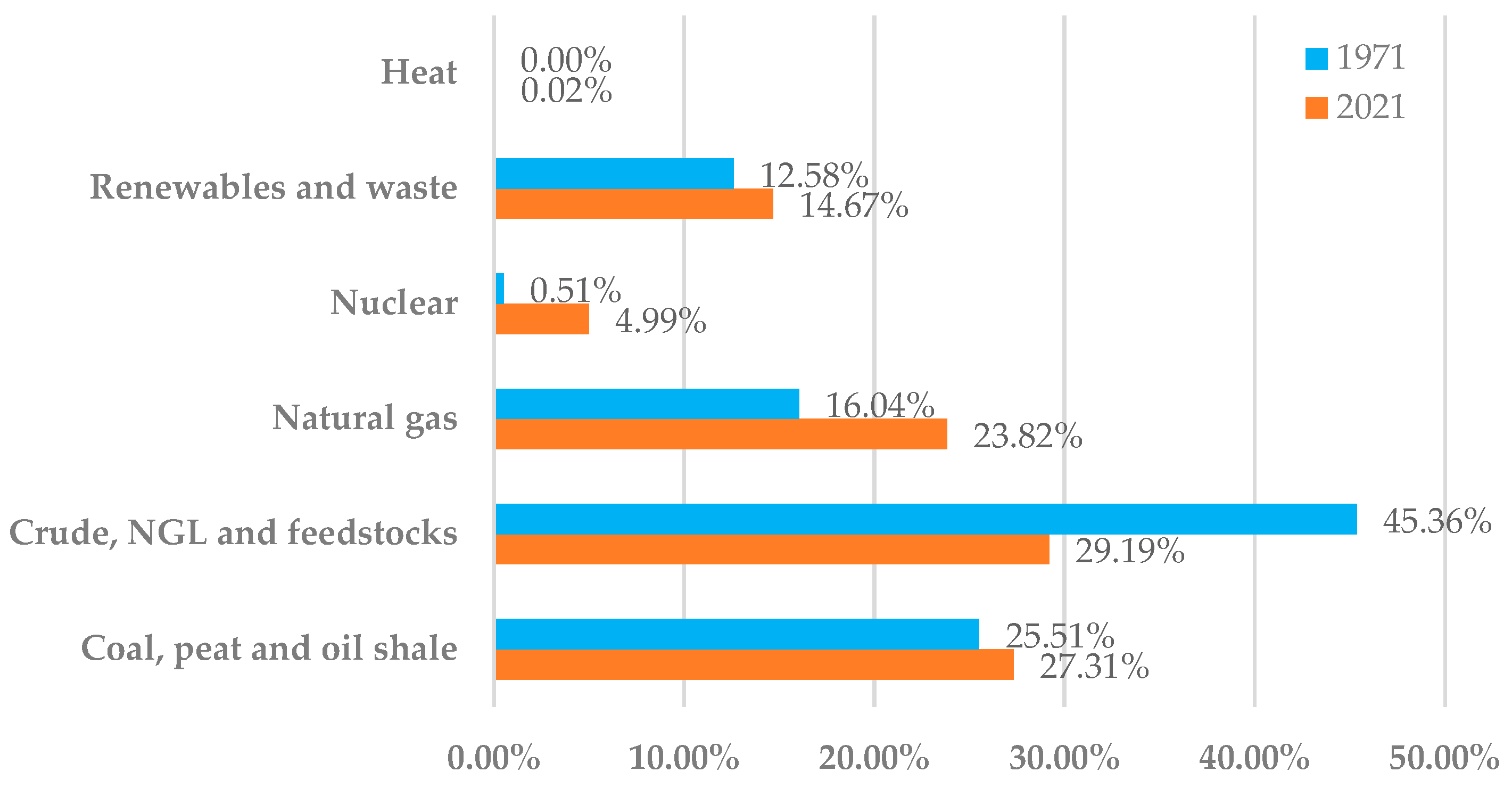
1.1. Types of Energy Resources
1.2. Industrial Waste
1.3. Biogas
1.4. Future Trends and Limitations of Bioenergy
2. Materials and Methods
- Categorical variable:
- ○
- Country from EU-27 (2020);
- ○
- Real GDP/capita (with the codification applied in SPSS 29.0 licensed software): 1 = below average EU yearly, 2 = above average EU yearly.
- Continuous variables:
- ○
- Real GDP/capita;
- ○
- Gross electricity production (GEP);
- ○
- Gross heat production (GHP);
- ○
- Production—total (PT);
- ○
- Production—imports (PI);
- ○
- Production—exports (PE);
- ○
- Production—stock exchange (PSE);
- ○
- Production—domestic supply (PDS);
- ○
- Transformation—total (TT);
- ○
- Transformation—electricity plants (TEP);
- ○
- Transformation—CHP plants (TCHPP);
- ○
- Transformation—heat plants (THP);
- ○
- Transformation—other transformation (TOT);
- ○
- Energy industry own use—total (EIOU);
- ○
- Final consumption—total (FC);
- ○
- Final consumption—industry (FCI);
- ○
- Final consumption—transport (FCT);
- ○
- Final consumption—residential (FCR);
- ○
- Final consumption—commercial and public services (FCCPC);
- ○
- Final consumption—agriculture/forestry (FCA).
- The descriptive statistics were used as mean ± standard deviation (minimum-maximum) for the continuous variables. By using descriptive statistics indicators, the extent to which differences and/or similarities occur can be observed, on the one hand, and the other hand, the chosen combination of statistical methods and machine learning methods is justified for the quantitative analysis as the core approach for all the research.
- To find out whether there is any statistically significant association between variables, the Pearson correlation coefficients were used to analyze the direction and intensity of the associations between these continuous variables inside each group of countries (</>EU average based on real GDP/capita), separately, for industrial waste and biogases. Only the statistical significance correlations were retained for p-value < 0.05.
- Inferential statistic tests were applied [58] to test whether there are statistically significant differences between the two groups of European Union countries (above average/below average of EU-27 based on real GDP/capita) referring to all variables from the study, separately, for industrial waste and biogases. The independent samples Mann–Whitney U test was used for the categorial variables used for comparisons, with p-value < 0.05.
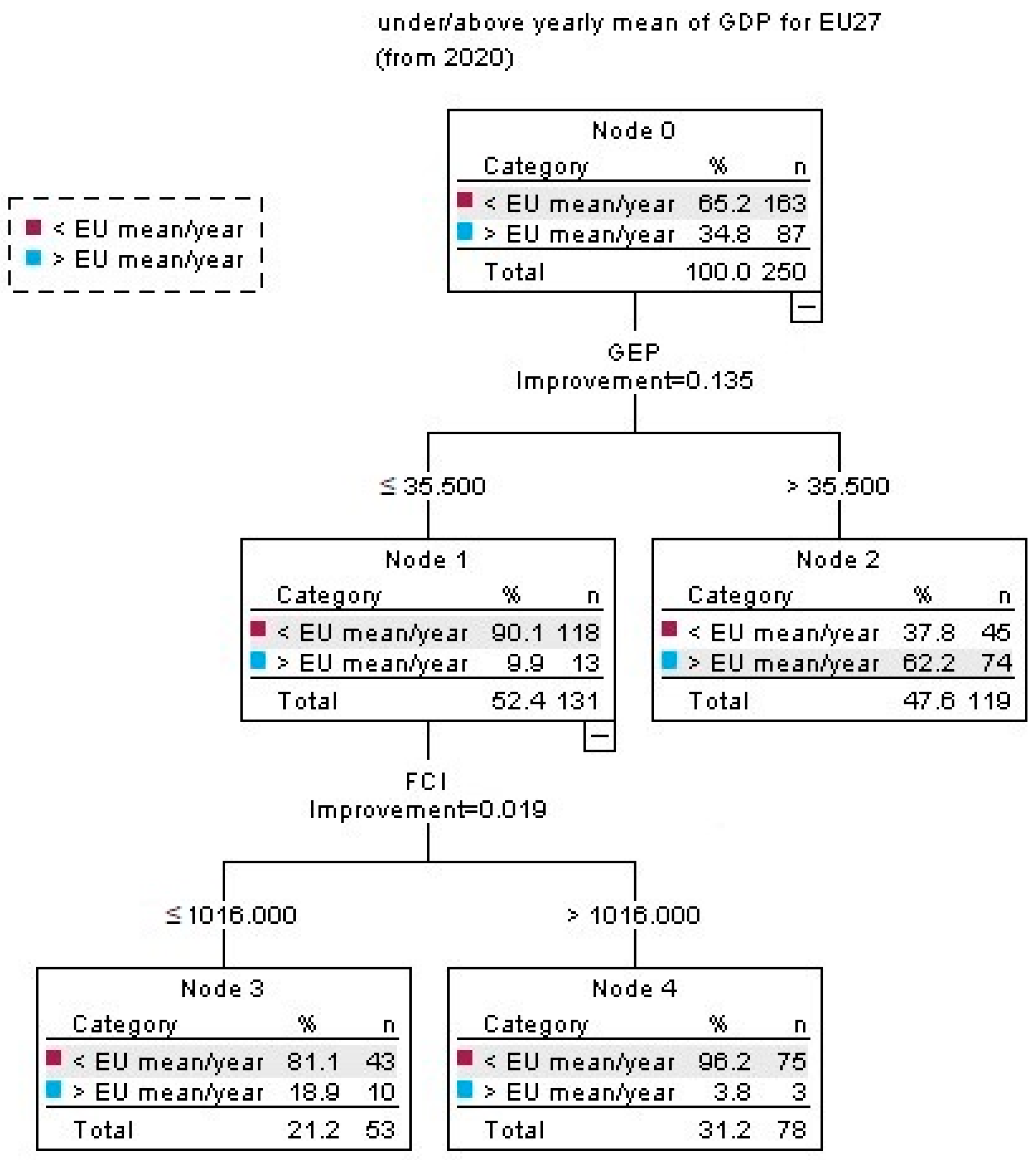
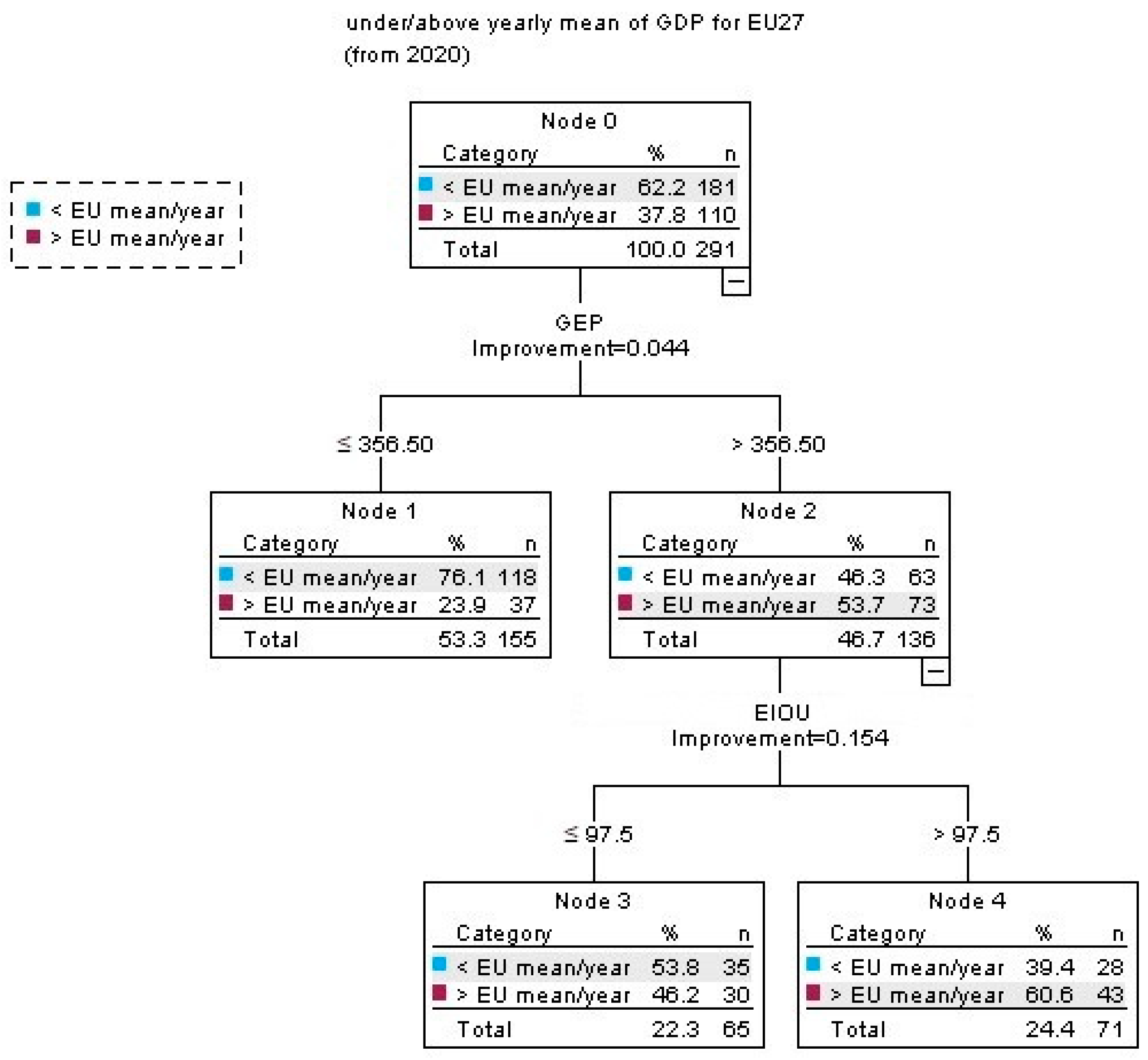
- A machine learning analysis based on the decision tree with CRT “growing method” was applied to find out which variables from the study could be grouped/separated better among EU-27 countries with real GDP/capita below/above the EU average. The statistical hypothesis for decision tree H0 is as follows: Variables are independent. The alternative hypothesis, H1, states the following: The variables are dependent. The main motivation for applying the decision tree with CRT is directly linked to the numerous advantages of this method, especially to the advantages of using decision tree compared to classical statistical methods [59,60,61,62], which are as follows: (1) the decision tree with CRT algorithm takes into consideration and presents the normalized importance of the independent variables; (2) it allows for the prediction of countries belonging to distinct categories based on their measures according to one or more predictor variables; (3) it allows for the utilization of both categorical or continuous types of data by using different algorithms (CHAID—Chi-square automatic interaction detection, CRT); (4) it groups/classifies the individuals/ideas into homogenous groups by one or more independent variables according to the importance of their contribution to the grouping process. Another important advantage of the decision tree is linked to the graphical representation of these groups and nodes based on the contribution of each independent variable to their formation.
3. Results and Discussion
- Data for these two variables are by far the most numerous and complete of all the other analyzed categories;
- The inclusion of all potential variables (already mentioned above) would require a very complicated analysis due to the nature of the data volume involved; in some places, the data cannot be unitarily compared to the other two components already included. This is the case when there is some missing information (in the case of some countries, some years, etc.), and this aspect can negatively influence the findings generated through the analysis for the industrial waste and biogas variables.
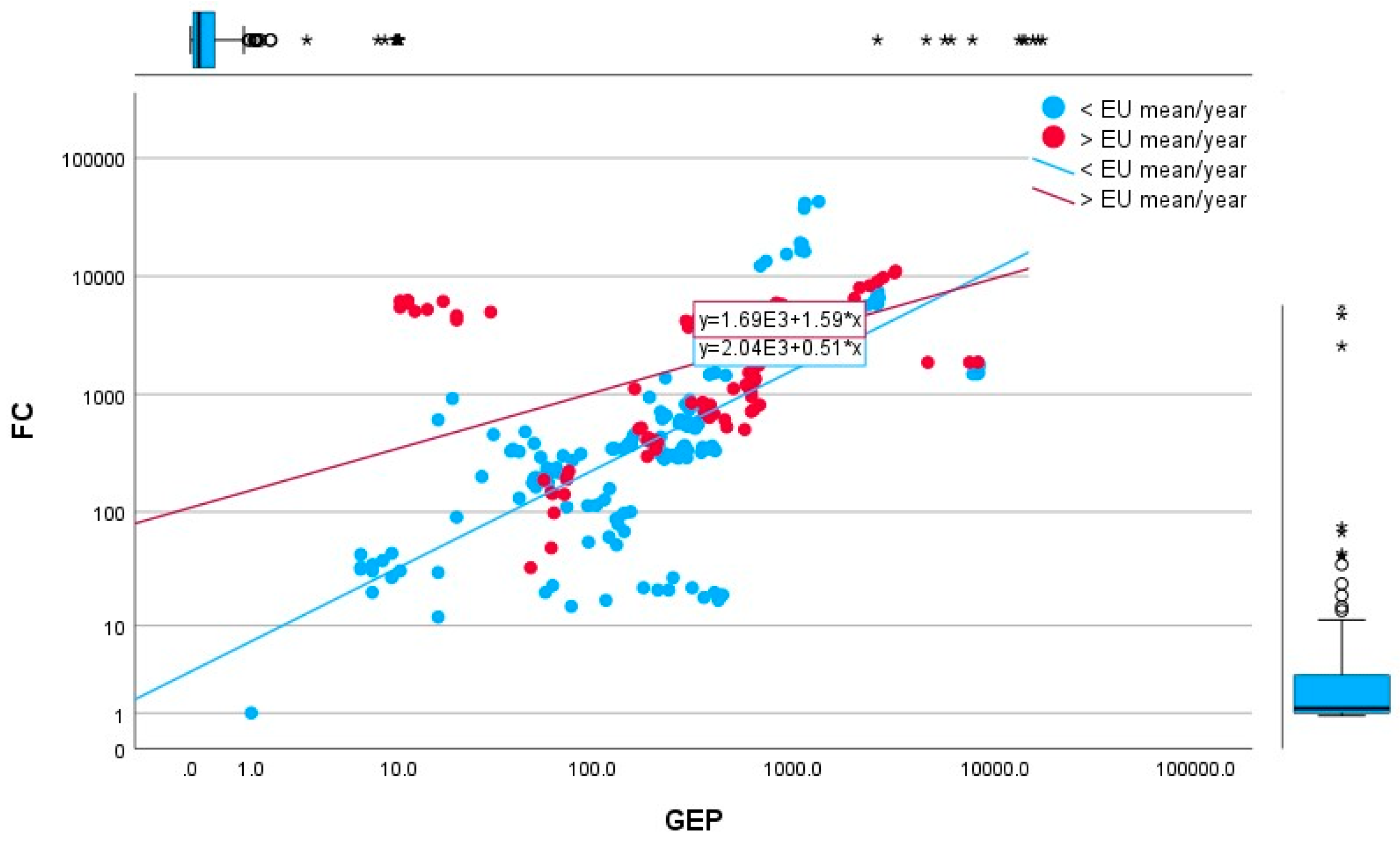
3.1. Industrial Waste
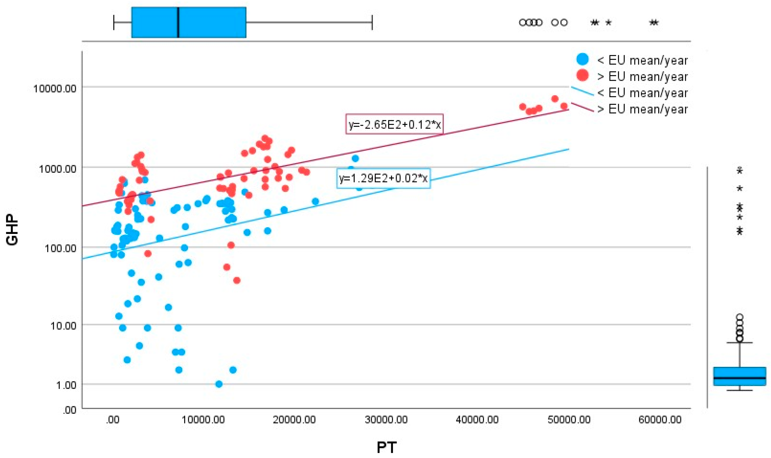
- Direct correlations of strong intensity between PT and FC (+0.993) and between GEP and TT (+0.873);
- Medium direct correlations between GHP and PT (+0.530), GHP and FC (+0.503), and real GDP/capita and TT (+0.442);
- Inverse correlations of medium intensity between real GDP/capita and EIOU (−0.424), GHP and EIOU (−0.485), and TT and EIOU (−0.418).
- Direct correlations of strong intensity between GEP and GHP (0.923), GEP and PT (0.934), GEP and FC (+0.814), GEP and TT (+0.883), GEP and EIOU (0.849), GHP and PT (0.917), GHP and FC (+0.833), PT and FC (+0.970), GHP and TT (+0.717), PT and TT (+0.799), and TT and EIOU (+0.751);
- Strong inverse correlations between real GDP/capita and EIOU (−0.804), GHP and EIOU (−0.753), PT and EIOU (−0.782), and EIOU and FC (−0.938).
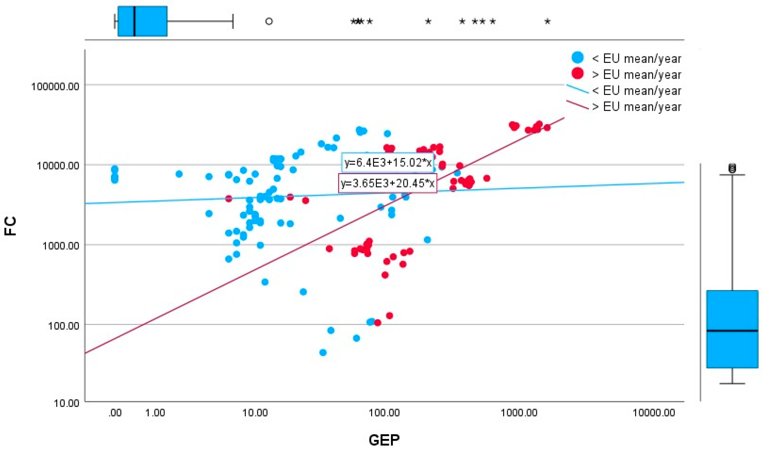
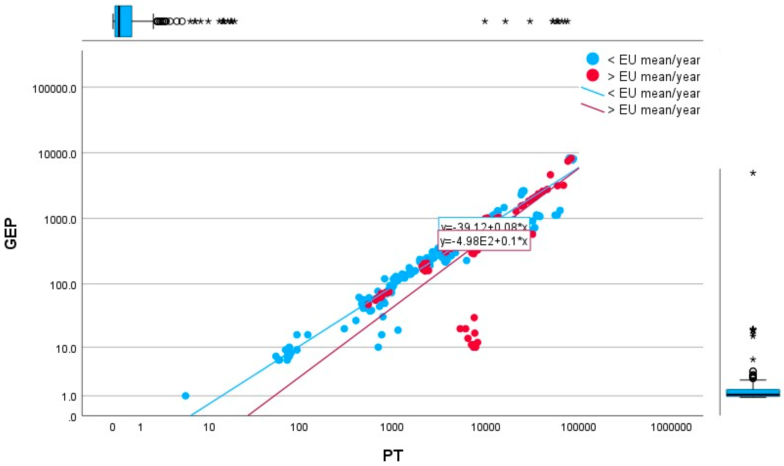
3.2. Biogases
4. Conclusions
- For industrial waste: FCI and FCCPS;
- For biogases: FCR, FCA, and TOT.
- For industrial waste: (1) for European countries with GDP/capita below the EU-27 average, there are direct and strong intensity correlations between PT and FC and between GEP and TT; (2) for European countries with GDP/capita higher the EU-27 average, there is a powerful direct correlation between most of the variables except for real GDP/capita and EIOU, with inverse medium to powerful correlations for all the rest of variables.
- For biogases: (1) for European countries with GDP/capita below the EU-27 average, there are strong direct correlations between GHP and GEP, GEP and PT, GEP and TT, GHP and PT, GHP, and TT, and PT and TT; (2) for European countries with GDP/capita higher the EU-27 average, there are direct and strong intensity correlations between all variables except real GDP/capita, but there is also an inverse correlation of strong intensity between real GDP/capita and EIOU.
- For industrial waste: the country distribution and the trend for the two groups of EU-27 countries are quite different, with a slow evolution for the group of EU-27 countries below average GDP, and a quite dynamic trend, with a positive slope for the group of EU-27 countries with higher GDP than average, with the exception of GHP depending by PT, where the evolution is quite similar.
- For biogases: the evolution and trend of GEP and GHP depending on PT is quite similar for both groups of countries, with a positive evolution. It is better for EU-27 countries with higher GDP/capita than for the group of EU-27 countries with lower GDP/capita for the distribution of GHP depending on PT. The trend for FC depending on GHP is also comparatively similar for the two groups of countries.
- The best predictor for groups of EU-27 countries with an average real GDP/capita per year higher/lower than the EU-27 average for both analyses for industrial waste is the GEP (with the cut-off = 35.5), followed by final consumption—industry (with a cut off = 1016.0), for countries with GEP < 35.5;
- The best predictor for groups of EU-27 countries with an average real GDP/capita per year higher/lower than the EU-27 average for both analyses for biogases is also the GEP (with the cut off = 356.5), followed by EIOU (with the cut off = 97.5), for countries with GEP > 356.5.
Author Contributions
Funding
Data Availability Statement
Conflicts of Interest
References
- The World Bank. Population Estimates and Projections 1971–2021. Available online: https://databank.worldbank.org/source/population-estimates-and-projections# (accessed on 1 April 2024).
- International Energy Agency. World Energy Balances 2023 Highlights. Available online: https://www.iea.org/data-and-statistics/data-product/world-energy-statistics-and-balances (accessed on 1 April 2024).
- UN Environment Programme. GOAL 7: Affordable and Clean Energy. Available online: https://www.unep.org/explore-topics/sustainable-development-goals/why-do-sustainable-development-goals-matter/goal-7 (accessed on 1 April 2024).
- International Energy Agency. Renewables 2023. Available online: https://www.iea.org/reports/renewables-2023 (accessed on 2 April 2024).
- International Energy Agency. Energy Statistics Data Browser 2023. Available online: https://www.iea.org/data-and-statistics/data-tools/energy-statistics-data-browser (accessed on 2 April 2024).
- International Energy Agency. Global Energy and Climate Model. Documentation—2023. Available online: https://www.iea.org/reports/global-energy-and-climate-model (accessed on 2 April 2024).
- Kalak, T. Potential Use of Industrial Biomass Waste as a Sustainable Energy Source in the Future. Energies 2023, 16, 1783. [Google Scholar] [CrossRef]
- Adeleke, O.; Akinlabi, S.A.; Jen, T.C.; Dunmade, I. Sustainable utilization of energy from waste: A review of potentials and challenges of Waste-to-energy in South Africa. Int. J. Green Energy 2021, 18, 1550–1564. [Google Scholar] [CrossRef]
- Odejobi, O.J.; Ajala, O.O.; Osuolale, F.N. Review on potential of using agricultural, municipal solid and industrial wastes as substrates for biogas production in Nigeria. Biomass Conv. Bioref. 2024, 14, 1567–1579. [Google Scholar] [CrossRef]
- Sharma, S.; Basu, S.; Shetti, N.P.; Aminabhavi, T.M. Waste-to-energy nexus for circular economy and environmental protection: Recent trends in hydrogen energy. Sci. Total Environ. 2020, 713, 136633. [Google Scholar] [CrossRef] [PubMed]
- Nomura, T.; Naimen, A.; Toyoda, S.; Kuriyama, Y.; Tokumoto, H.; Konishi, Y. Isolation and characterization of a novel hydrogen-producing strain Clostridium sp. suitable for immobilization. Int. J. Hydrogen Energy 2014, 39, 1280–1287. [Google Scholar] [CrossRef]
- Błaszczyk, A.; Sady, S.; Pachołek, B.; Jakubowska, D.; Grzybowska-Brzezińska, M.; Krzywonos, M.; Popek, S. Sustainable Management Strategies for Fruit Processing Byproducts for Biorefineries: A Review. Sustainability 2024, 16, 1717. [Google Scholar] [CrossRef]
- Feng, X.; Wang, H.; Wang, Y.; Wang, X.; Huang, J. Biohydrogen production from apple pomace by anaerobic fermentation with river sludge. Int. J. Hydrogen Energy 2010, 35, 3058–3064. [Google Scholar] [CrossRef]
- Singh, T.; Alhazmi, A.; Mohammad, A.; Srivastava, N.; Haque, S.; Sharma, S.; Singh, R.; Yoon, T.; Gupta, V.K. Integrated biohydrogen production via lignocellulosic waste: Opportunity, challenges & future prospects. Bioresour. Technol. 2021, 338, 125511. [Google Scholar] [CrossRef]
- Yaashikaa, P.R.; Senthil Kumar, P.; Varjani, S. Valorization of agro-industrial wastes for biorefinery process and circular bioeconomy: A critical review. Bioresour. Technol. 2022, 343, 126126. [Google Scholar] [CrossRef]
- Chung, T.H.; Dhar, B.R. A multi-perspective review on microbial electrochemical technologies for food waste valorisation. Bioresour. Technol. 2021, 342, 125950. [Google Scholar] [CrossRef]
- Gupta, S.; Patro, A.; Mittal, Y.; Dwivedi, S.; Saket, P.; Panja, R.; Saeed, T.; Martínez, F.; Yadav, A.K. The race between classical microbial fuel cells, sediment-microbial fuel cells, plant-microbial fuel cells, and constructed wetlands-microbial fuel cells: Applications and technology readiness level. Sci. Total Environ. 2023, 879, 162757. [Google Scholar] [CrossRef] [PubMed]
- Goren, A.Y.; Okten, H.E. Energy production from treatment of industrial wastewater and boron removal in aqueous solutions using microbial desalination cell. Chemosphere 2021, 285, 131370. [Google Scholar] [CrossRef]
- Zahid, M.; Savla, N.; Pandit, S.; Thakur, V.K.; Jung, S.P.; Gupta, P.K.; Prasad, R.; Marsili, E. Microbial desalination cell: Desalination through conserving energy. Desalination 2022, 521, 115381. [Google Scholar] [CrossRef]
- Cusick, R.D.; Kim, Y.; Logan, B.E. Energy Capture from Thermolytic Solutions in Microbial Reverse-Electrodialysis Cells. Science 2012, 335, 1474–1477. [Google Scholar] [CrossRef] [PubMed]
- Jung, S.; Shetti, N.P.; Reddy, K.R.; Nadagouda, M.N.; Park, Y.-K.; Aminabhavi, T.M.; Kwon, E.E. Synthesis of different biofuels from livestock waste materials and their potential as sustainable feedstocks—A review. Energy Convers. Manag. 2021, 236, 114038. [Google Scholar] [CrossRef]
- Purnomo, C.W.; Kurniawan, W.; Aziz, M. Technological review on thermochemical conversion of COVID-19-related medical wastes. Resour. Conserv. Recycl. 2021, 167, 105429. [Google Scholar] [CrossRef]
- Felix, C.B.; Ubando, A.T.; Chen, W.-H.; Goodarzi, V.; Ashokkumar, V. COVID-19 and industrial waste mitigation via thermochemical technologies towards a circular economy: A state-of-the-art review. J. Hazard. Mater. 2022, 423, 127215. [Google Scholar] [CrossRef]
- Rafiee, A.; Khalilpour, K.R.; Prest, J.; Skryabin, I. Biogas as an energy vector. Biomass Bioenergy 2021, 144, 105935. [Google Scholar] [CrossRef]
- Nwokolo, N.; Mukumba, P.; Obileke, K.; Enebe, M. Waste to Energy: A Focus on the Impact of Substrate Type in Biogas Production. Processes 2020, 8, 1224. [Google Scholar] [CrossRef]
- Ignatowicz, K.; Filipczak, G.; Dybek, B.; Wałowski, G. Biogas Production Depending on the Substrate Used: A Review and Evaluation Study—European Examples. Energies 2023, 16, 798. [Google Scholar] [CrossRef]
- AL-Huqail, A.A.; Kumar, V.; Kumar, R.; Eid, E.M.; Taher, M.A.; Adelodun, B.; Abou Fayssal, S.; Mioč, B.; Držaić, V.; Goala, M.; et al. Sustainable Valorization of Four Types of Fruit Peel Waste for Biogas Recovery and Use of Digestate for Radish (Raphanus sativus L. cv. Pusa Himani) Cultivation. Sustainability 2022, 14, 10224. [Google Scholar] [CrossRef]
- Mavridis, S.; Voudrias, E.A. Using biogas from municipal solid waste for energy production: Comparison between anaerobic digestion and sanitary landfilling. Energy Convers. Manag. 2021, 247, 114613. [Google Scholar] [CrossRef]
- Kasinath, A.; Fudala-Ksiazek, S.; Szopinska, M.; Bylinski, H.; Artichowicz, W.; Remiszewska-Skwarek, A.; Luczkiewicz, A. Biomass in biogas production: Pretreatment and codigestion. Renew. Sustain. Energy Rev. 2021, 150, 111509. [Google Scholar] [CrossRef]
- Stürmer, B.; Leiers, D.; Anspach, V.; Brügging, E.; Scharfy, D.; Wissel, T. Agricultural biogas production: A regional comparison of technical parameters. Renew. Energy 2021, 164, 171–182. [Google Scholar] [CrossRef]
- O’Connor, S.; Ehimen, E.; Pillai, S.C.; Black, A.; Tormey, D.; Bartlett, J. Biogas production from small-scale anaerobic digestion plants on European farms. Renew. Sustain. Energy Rev. 2021, 139, 110580. [Google Scholar] [CrossRef]
- Ceylan, A.B.; Aydın, L.; Nil, M.; Mamur, H.; Polatoğlu, İ.; Sözen, H. A new hybrid approach in selection of optimum establishment location of the biogas energy production plant. Biomass Convers. Biorefin. 2023, 13, 5771–5786. [Google Scholar] [CrossRef]
- Afotey, B.; Sarpong, G.T. Estimation of biogas production potential and greenhouse gas emissions reduction for sustainable energy management using intelligent computing technique. Meas. Sens. 2023, 25, 100650. [Google Scholar] [CrossRef]
- Kamalov, F.; Santandreu Calonge, D.; Gurrib, I. New Era of Artificial Intelligence in Education: Towards a Sustainable Multifaceted Revolution. Sustainability 2023, 15, 12451. [Google Scholar] [CrossRef]
- Rosca, C.M.; Ariciu, A.V. Unlocking Customer Sentiment Insights with Azure Sentiment Analysis: A Comprehensive Review and Analysis. Rom. J. Pet. Gas Technol. 2023, IV, 173–182. [Google Scholar] [CrossRef]
- Oluleye, B.I.; Chan, D.W.M.; Antwi-Afari, P. Adopting Artificial Intelligence for enhancing the implementation of systemic circularity in the construction industry: A critical review. Sustain. Prod. Consum. 2023, 35, 509–524. [Google Scholar] [CrossRef]
- Lăzăroiu, G.; Bogdan, M.; Geamănu, M.; Hurloiu, L.; Luminița, L.; Ștefănescu, R. Artificial intelligence algorithms and cloud computing technologies in blockchain-based fintech management. Oecon. Copernic. 2023, 14, 707–730. [Google Scholar] [CrossRef]
- Androniceanu, A. The new trends of digital transformation and artificial intelligence in public administration. Adm. Si Manag. Public 2023, 40, 147–155. [Google Scholar] [CrossRef]
- Al-Antari, M.A. Artificial Intelligence for Medical Diagnostics—Existing and Future AI Technology! Diagnostics 2023, 13, 688. [Google Scholar] [CrossRef] [PubMed]
- Rosca, C.M. Comparative Analysis of Object Classification Algorithms: Traditional Image Processing Versus Artificial Intelligence—Based Approach. Rom. J. Pet. Gas Technol. 2023, IV, 169–180. [Google Scholar] [CrossRef]
- Huang, Q.; Peng, S.; Deng, J.; Zeng, H.; Zhang, Z.; Liu, Y.; Yuan, P. A review of the application of artificial intelligence to nuclear reactors: Where we are and what’s next. Heliyon 2023, 9, e13883. [Google Scholar] [CrossRef] [PubMed]
- Jin, H.; Kim, Y.-G.; Jin, Z.; Rushchitc, A.A.; Al-Shati, A.S. Optimization and analysis of bioenergy production using machine learning modeling: Multi-layer perceptron, Gaussian processes regression, K-nearest neighbors, and Artificial neural network models. Energy Rep. 2022, 8, 13979–13996. [Google Scholar] [CrossRef]
- Senocak, A.A.; Guner Goren, H. Forecasting the biomass-based energy potential using artificial intelligence and geographic information systems: A case study. Eng. Sci. Technol. Int. J. 2022, 26, 100992. [Google Scholar] [CrossRef]
- Sahoo, A.; Saini, K.; Negi, S.; Kumar, J.; Pant, K.K.; Bhaskar, T. Inspecting the bioenergy potential of noxious Vachellia nilotica weed via pyrolysis: Thermo-kinetic study, neural network modeling and response surface optimization. Renew. Energy 2022, 185, 386–402. [Google Scholar] [CrossRef]
- Singh, P.K.; Chauhan, S.S.; Sharma, A.; Prakash, S.; Singh, Y. Prediction of higher heating values based on imminent analysis by using regression analysis and artificial neural network for bioenergy resources. Proc. Inst. Mech. Eng. Part E J. Process Mech. Eng. 2023, 09544089231175046. [Google Scholar] [CrossRef]
- Pereira, R.D.; Badino, A.C.; Cruz, A.J.G. Framework Based on Artificial Intelligence to Increase Industrial Bioethanol Production. Energy Fuels 2020, 34, 4670–4677. [Google Scholar] [CrossRef]
- Carrijo, J.V.N.; Miguel, E.P.; Teixeira Do Vale, A.; Matricardi, E.A.T.; Monteiro, T.C.; Rezende, A.V.; Inkotte, J. Artificial intelligence associated with satellite data in predicting energy potential in the Brazilian savanna woodland area. iForest—Biogeosciences For. 2020, 13, 48–55. [Google Scholar] [CrossRef]
- Cinar, S.; Cinar, S.O.; Wieczorek, N.; Sohoo, I.; Kuchta, K. Integration of Artificial Intelligence into Biogas Plant Operation. Processes 2021, 9, 85. [Google Scholar] [CrossRef]
- Huang, Y.; Partha, D.B.; Harper, K.; Heyes, C. Impacts of Global Solid Biofuel Stove Emissions on Ambient Air Quality and Human Health. Geohealth 2021, 5, e2020GH000362. [Google Scholar] [CrossRef]
- Irmak, S. Challenges of Biomass Utilization for Biofuels. In Biomass for Bioenergy—Recent Trends and Future Challenges; Abomohra, A.E., Ed.; IntechOpen: London, UK, 2019; pp. 1–11. [Google Scholar]
- Torkashvand, M.; Hasan-Zadeh, A.; Torkashvand, A. Mini Review on Importance, Application, Advantages and Disadvantages of Biofuels. J. Mater. Environ. Sci. 2022, 13, 612–630. [Google Scholar]
- Matei, M.; Done, I.; Andrei, J.-V.; Ene, C.; Stancu, A. Some Disadvantages of Biofuels Production Using Agricultural Products. In Proceedings of the International Scientific Meeting “Multifunctional Agriculture and Rural Development (III)—Rural Development and (Un)Limited Resources”, Belgrade, Serbia, 4–5 December 2008; First Book. Institute of Agricultural Economics Belgrade: Belgrade, Serbia, 2008; pp. 97–103. [Google Scholar]
- Das, J.; Ravishankar, H.; Lens, P.N.L. Biological biogas purification: Recent developments, challenges and future prospects. J. Environ. Manag. 2022, 304, 114198. [Google Scholar] [CrossRef]
- Ocak, S.; Acar, S. Biofuels from wastes in Marmara Region, Turkey: Potentials and constraints. Environ. Sci. Pollut. Res. 2021, 28, 66026–66042. [Google Scholar] [CrossRef]
- Ene, C.; Stancu, A. Impact of Biofuels Production on Food Security on Selected African Countries. In Energy Transition. Economic, Social and Environmental Dimensions; Khan, S.A.R., Panait, M., Puime Guillen, F., Raimi, L., Eds.; Springer: Singapore, 2022; pp. 215–248. ISBN 978-981-19-3539-8. [Google Scholar] [CrossRef]
- International Energy Agency. Energy Statistics Manual 2004. Available online: https://iea.blob.core.windows.net/assets/67fb0049-ec99-470d-8412-1ed9201e576f/EnergyStatisticsManual.pdf (accessed on 15 April 2024).
- Eurostat. Real GDP per Capita, 2024. Available online: https://ec.europa.eu/eurostat/databrowser/view/sdg_08_10/default/table (accessed on 15 April 2024).
- Gabor, M.R. Analiza și Inferența Datelor de Marketing (Analysis and Inference of Marketing Data); C.H. Beck: Bucharest, Romania, 2016. [Google Scholar]
- McCormik, K.; Salcedo, J.; Peck, J.; Wheeler, A. SPSS Statistics for Data Analysis and Visualization; John Wiley & Sons: Indianapolis, IN, USA, 2017; pp. 355–392. [Google Scholar]
- Petcu, N. Tehnici de Data Mining Rezolvate in SPSS Clementine; Albastra: Cluj-Napoca, Romania, 2010; p. 81. [Google Scholar]
- Gorunescu, F. Data Mining—Concepte, Modele și Tehnici; Albastra: Cluj-Napoca, Romania, 2006; p. 142. [Google Scholar]
- Rakotomalala, R. Les Methodes d’Induction d’Arbres; Laboratoire ERIC: Lyon, France, 2005. [Google Scholar]


| Variables | <EU-27 Average | >EU-27 Average | ||||||||
|---|---|---|---|---|---|---|---|---|---|---|
| Mean | Median | Std. Deviation | Minimum | Maximum | Mean | Median | Std. Deviation | Minimum | Maximum | |
| Real GDP/capita | 15,632.06 | 14,920.00 | 7508.82 | 5390.00 | 81,940 | 41,793.10 | 36,220.00 | 15,768.19 | 25,620.00 | 86,540.00 |
| GEP | 51.89 | 16.00 | 69.22 | 0.00 | 345.00 | 312.14 | 181.00 | 378.95 | 6.00 | 1604.00 |
| GHP | 245.52 | 184.50 | 217.08 | 1.00 | 1281.00 | 1595.04 | 748.00 | 2114.85 | 38.00 | 9741.00 |
| PT | 5004.83 | 2395.00 | 6241.03 | 9.00 | 28,437.00 | 13,739.40 | 12,156.00 | 15,844.16 | 546.00 | 59,472.00 |
| PI | 742.79 | 330.00 | 842.65 | 1.00 | 3369.00 | |||||
| PSE | 5.20 | 1.00 | 57.73 | −142.00 | 171.00 | 50,887.00 | 49,437.00 | 5212.80 | 44,922.00 | 59,472.00 |
| PDS | 5215.65 | 2597.00 | 6203.12 | 11.00 | 28,437.00 | 9989.49 | 12,156.00 | 8246.19 | 546.00 | 30,439.00 |
| TT | 733.45 | 410.00 | 801.48 | 1.00 | 4811.00 | 3964.65 | 3274.50 | 2710.18 | 126.00 | 11,569.00 |
| TEP | 560.64 | 274.50 | 915.92 | 0.00 | 4806.00 | 2511.30 | 848.00 | 3794.81 | 0.00 | 15,764.00 |
| TCHPP | 439.34 | 335.00 | 362.27 | 5.00 | 1758.00 | 2420.88 | 1735.00 | 1877.04 | 222.00 | 6253.00 |
| THP | 238.20 | 178.50 | 240.92 | 1.00 | 938.00 | 546.38 | 605.00 | 439.68 | 27.00 | 1367.00 |
| EIOU | 524.15 | 284.00 | 711.87 | 1.00 | 2828.00 | 3691.83 | 1936.00 | 2653.37 | 597.00 | 7564.00 |
| FC | 5118.27 | 2702.00 | 6020.05 | 2.00 | 27,296.00 | 9410.53 | 6349.00 | 9706.78 | 105.00 | 32,173.00 |
| FCI | 6340.35 | 4005.00 | 6229.20 | 44.00 | 27,159.00 | 9657.76 | 7411.50 | 10,128.03 | 105.00 | 32,173.00 |
| FCCPS | 3280.58 | 167.00 | 4522.79 | 1.00 | 11,291.00 | 396.36 | 111.00 | 504.74 | 8.00 | 1200.00 |
| Null Hypothesis | Test | Sig. a,b | Decision |
|---|---|---|---|
| The distribution of FCI is the same across categories under/above the yearly mean of GDP for EU-27 (from 2020). | Independent samples Mann–Whitney U test | 0.160 | Retain the null hypothesis. |
| The distribution of FCCPS is the same across categories under/above the yearly mean of GDP for EU-27 (from 2020). | Independent samples Mann–Whitney U test | 0.050 | Retain the null hypothesis. |
| Under/Above the Yearly Mean of GDP for EU-27 (from 2020) | Real GDP/Capita | GEP | GHP | PT | TT | EIOU | FC | ||
|---|---|---|---|---|---|---|---|---|---|
| <EU mean/year | Real GDP/capita | Pearson Correlation | 1 | 0.233 * | 0.212 * | 0.102 | 0.442 ** | −0.424 ** | 0.078 |
| Sig. (2-tailed) | 0.014 | 0.045 | 0.193 | <0.001 | 0.003 | 0.351 | |||
| N | 165 | 110 | 90 | 163 | 112 | 48 | 147 | ||
| GEP | Pearson Correlation | 1 | 0.533 ** | 0.151 | 0.873 ** | −0.485 * | 0.149 | ||
| Sig. (2-tailed) | <0.001 | 0.116 | <0.001 | 0.041 | 0.149 | ||||
| N | 110 | 77 | 110 | 99 | 18 | 95 | |||
| GHP | Pearson Correlation | 1 | 0.530 ** | 0.706 ** | −0.283 | 0.503 ** | |||
| Sig. (2-tailed) | <0.001 | <0.001 | 0.227 | <0.001 | |||||
| N | 90 | 90 | 85 | 20 | 83 | ||||
| PT | Pearson Correlation | 1 | 0.332 ** | −0.334 * | 0.993 ** | ||||
| Sig. (2-tailed) | <0.001 | 0.020 | <0.001 | ||||||
| N | 163 | 112 | 48 | 147 | |||||
| TT | Pearson Correlation | 1 | −0.418 | 0.240 * | |||||
| Sig. (2-tailed) | 0.084 | 0.016 | |||||||
| N | 112 | 18 | 100 | ||||||
| EIOU | Pearson Correlation | 1 | −0.351 * | ||||||
| Sig. (2-tailed) | 0.015 | ||||||||
| N | 48 | 47 | |||||||
| FC | Pearson Correlation | 1 | |||||||
| Sig. (2-tailed) | |||||||||
| N | 147 | ||||||||
| >EU mean/year | Real GDP/capita | Pearson Correlation | 1 | −0.262 * | −0.145 | −0.386 ** | −0.232 | −0.804 ** | −0.416 ** |
| Sig. (2-tailed) | 0.022 | 0.209 | <0.001 | 0.057 | <0.001 | <0.001 | |||
| N | 87 | 77 | 77 | 87 | 68 | 18 | 79 | ||
| GEP | Pearson Correlation | 1 | 0.923 ** | 0.934 ** | 0.883 ** | 0.849 ** | 0.814 ** | ||
| Sig. (2-tailed) | <0.001 | <0.001 | <0.001 | <0.001 | <0.001 | ||||
| N | 77 | 77 | 77 | 68 | 18 | 69 | |||
| GHP | Pearson Correlation | 1 | 0.917 ** | 0.717 ** | −0.753 ** | 0.833 ** | |||
| Sig. (2-tailed) | <0.001 | <0.001 | <0.001 | <0.001 | |||||
| N | 77 | 77 | 68 | 18 | 69 | ||||
| PT | Pearson Correlation | 1 | 0.799 ** | −0.782 ** | 0.970 ** | ||||
| Sig. (2-tailed) | <0.001 | <0.001 | <0.001 | ||||||
| N | 87 | 68 | 18 | 79 | |||||
| TT | Pearson Correlation | 1 | 0.751 ** | 0.669 ** | |||||
| Sig. (2-tailed) | <0.001 | <0.001 | |||||||
| N | 68 | 18 | 68 | ||||||
| EIOU | Pearson Correlation | 1 | −0.938 ** | ||||||
| Sig. (2-tailed) | <0.001 | ||||||||
| N | 18 | 18 | |||||||
| FC | Pearson Correlation | 1 | |||||||
| Sig. (2-tailed) | |||||||||
| N | 79 | ||||||||
| Variables | <EU-27 Average | >EU-27 Average | ||||||||
|---|---|---|---|---|---|---|---|---|---|---|
| Mean | Median | Std. Deviation | Minimum | Maximum | Mean | Median | Std. Deviation | Minimum | Maximum | |
| GHP | 1221.96 | 186.00 | 2648.447 | 1 | 12,177 | 2036.45 | 526.00 | 3655.369 | 46 | 18,103 |
| PT | 10,342.46 | 3323.00 | 18,900.855 | 5 | 87,007 | 42,728.31 | 9089.00 | 90,514.681 | 548 | 325,115 |
| PI | 193.58 | 33.00 | 337.356 | 3 | 1000 | 79.00 | 79.00 | 79 | 79 | |
| PE | −510.40 | −491.00 | 87.500 | −687 | −393 | |||||
| PSE | −15.40 | 31.50 | 161.305 | −410 | 158 | |||||
| PDS | 10,326.24 | 3323.00 | 18,865.954 | 5 | 87,007 | 42,729.03 | 9089.00 | 90,514.393 | 548 | 325,115 |
| TT | 7856.56 | 2474.00 | 16,723.638 | 4 | 85,520 | 32,383.95 | 5841.00 | 68,811.016 | 358 | 248,072 |
| TEP | 3014.78 | 527.00 | 6831.503 | 3 | 30,711 | 12,635.93 | 1648.50 | 24,206.839 | 1 | 90,483 |
| TCHPP | 5353.52 | 1223.00 | 10,689.690 | 28 | 55,291 | 18,352.02 | 3432.00 | 43,862.868 | 182 | 179,407 |
| THP | 503.51 | 17.00 | 1022.021 | 1 | 2953 | 192.63 | 139.00 | 150.076 | 1 | 588 |
| TOT | 1094.32 | 303.00 | 2002.054 | 25 | 7769 | 3726.01 | 467.50 | 7235.062 | 2 | 33,549 |
| EIOU | 281.08 | 38.00 | 713.252 | 1 | 4597 | 7216.65 | 756.00 | 9306.207 | 56 | 21,429 |
| FC | 2464.67 | 345.50 | 6073.278 | 1 | 42,861 | 7995.70 | 3679.00 | 15,282.926 | 33 | 59,721 |
| FCI | 1331.04 | 217.00 | 3562.582 | 1 | 17,055 | 1276.93 | 1230.00 | 942.790 | 22 | 3672 |
| FCT | 205.64 | 1.00 | 331.896 | 1 | 1,000 | 1138.98 | 59.00 | 1575.262 | 1 | 4960 |
| FCR | 8715.80 | 1543.00 | 11,825.152 | 1021 | 28,680 | 4839.61 | 1586.50 | 5300.883 | 1 | 13,156 |
| FCCPC | 497.18 | 129.00 | 746.924 | 1 | 2899 | 2660.24 | 770.50 | 4732.878 | 2 | 17,268 |
| FCA | 812.57 | 183.00 | 1628.567 | 1 | 5741 | 3540.49 | 183.00 | 7364.856 | 1 | 25,594 |
| Null Hypothesis | Test | Sig. a,b | Decision |
|---|---|---|---|
| The distribution of TOT is the same across categories under/above the yearly mean of GDP for EU-27 (from 2020). | Independent samples Mann–Whitney U test | 0.169 | Retain the null hypothesis. |
| The distribution of FCR is the same across categories under/above the yearly mean of GDP for EU-27 (from 2020). | Independent samples Mann–Whitney U test | 0.272 | Retain the null hypothesis. |
| The distribution of FCA is the same across categories under/above the yearly mean of GDP for EU27 (from 2020). | Independent samples Mann–Whitney U test | 0.174 | Retain the null hypothesis. |
| Under/Above the Yearly Mean of GDP for EU-27 (from 2020) | Real GDP/Capita | GEP | GHP | PT | TT | EIOU | FC | ||
|---|---|---|---|---|---|---|---|---|---|
| <EU mean/year | Real GDP/capita | Pearson Correlation | -- | ||||||
| Sig. (2-tailed) | |||||||||
| N | 181 | ||||||||
| GEP | Pearson Correlation | 0.317 ** | -- | ||||||
| Sig. (2-tailed) | <0.001 | ||||||||
| N | 181 | 181 | |||||||
| GHP | Pearson Correlation | 0.283 ** | 0.840 ** | -- | |||||
| Sig. (2-tailed) | <0.001 | <0.001 | |||||||
| N | 144 | 144 | 144 | ||||||
| PT | Pearson Correlation | 0.280 ** | 0.914 ** | 0.946 ** | -- | ||||
| Sig. (2-tailed) | <0.001 | <0.001 | <0.001 | ||||||
| N | 181 | 181 | 144 | 181 | |||||
| PP | Pearson Correlation | 0.315 ** | 0.986 ** | 0.916 ** | 0.948 ** | -- | |||
| Sig. (2-tailed) | <0.001 | <0.001 | <0.001 | <0.001 | |||||
| N | 179 | 179 | 142 | 179 | 179 | ||||
| EIOU | Pearson Correlation | 0.251 | 0.274 | −0.318 | 0.137 | 0.105 | -- | ||
| Sig. (2-tailed) | 0.082 | 0.057 | 0.076 | 0.347 | 0.472 | ||||
| N | 49 | 49 | 32 | 49 | 49 | 49 | |||
| FC | Pearson Correlation | 0.007 | 0.144 | 0.418 ** | 0.511 ** | 0.212 ** | 0.023 | -- | |
| Sig. (2-tailed) | 0.928 | 0.054 | <0.001 | <0.001 | 0.004 | 0.873 | |||
| N | 178 | 178 | 141 | 178 | 178 | 49 | 178 | ||
| >EU mean/year | Real GDP/capita | Pearson Correlation | -- | ||||||
| Sig. (2-tailed) | |||||||||
| N | 110 | ||||||||
| GEP | Pearson Correlation | −0.236 * | -- | ||||||
| Sig. (2-tailed) | 0.013 | ||||||||
| N | 110 | 110 | |||||||
| GHP | Pearson Correlation | −0.261 ** | 0.876 ** | -- | |||||
| Sig. (2-tailed) | 0.009 | <0.001 | |||||||
| N | 99 | 99 | 99 | ||||||
| PT | Pearson Correlation | −0.252 ** | 0.997 ** | 0.884 ** | -- | ||||
| Sig. (2-tailed) | 0.008 | <0.001 | <0.001 | ||||||
| N | 110 | 110 | 99 | 110 | |||||
| TT | Pearson Correlation | −0.252 ** | 0.994 ** | 0.892 ** | 0.999 ** | -- | |||
| Sig. (2-tailed) | 0.008 | <0.001 | <0.001 | <0.001 | |||||
| N | 110 | 110 | 99 | 110 | 110 | ||||
| EIOU | Pearson Correlation | −0.895 ** | 0.998 ** | 0.848 ** | 0.996 ** | 0.993 ** | -- | ||
| Sig. (2-tailed) | <0.001 | <0.001 | <0.001 | <0.001 | <0.001 | ||||
| N | 31 | 31 | 31 | 31 | 31 | 31 | |||
| FC | Pearson Correlation | −0.266 ** | 0.983 ** | 0.852 ** | 0.983 ** | 0.972 ** | 0.991 ** | -- | |
| Sig. (2-tailed) | 0.005 | <0.001 | <0.001 | <0.001 | <0.001 | <0.001 | |||
| N | 109 | 109 | 99 | 109 | 109 | 31 | 109 | ||
Disclaimer/Publisher’s Note: The statements, opinions and data contained in all publications are solely those of the individual author(s) and contributor(s) and not of MDPI and/or the editor(s). MDPI and/or the editor(s) disclaim responsibility for any injury to people or property resulting from any ideas, methods, instructions or products referred to in the content. |
© 2024 by the authors. Licensee MDPI, Basel, Switzerland. This article is an open access article distributed under the terms and conditions of the Creative Commons Attribution (CC BY) license (https://creativecommons.org/licenses/by/4.0/).
Share and Cite
Popescu, C.; Gabor, M.R.; Stancu, A. Predictors for Green Energy vs. Fossil Fuels: The Case of Industrial Waste and Biogases in European Union Context. Agronomy 2024, 14, 1459. https://doi.org/10.3390/agronomy14071459
Popescu C, Gabor MR, Stancu A. Predictors for Green Energy vs. Fossil Fuels: The Case of Industrial Waste and Biogases in European Union Context. Agronomy. 2024; 14(7):1459. https://doi.org/10.3390/agronomy14071459
Chicago/Turabian StylePopescu, Catalin, Manuela Rozalia Gabor, and Adrian Stancu. 2024. "Predictors for Green Energy vs. Fossil Fuels: The Case of Industrial Waste and Biogases in European Union Context" Agronomy 14, no. 7: 1459. https://doi.org/10.3390/agronomy14071459
APA StylePopescu, C., Gabor, M. R., & Stancu, A. (2024). Predictors for Green Energy vs. Fossil Fuels: The Case of Industrial Waste and Biogases in European Union Context. Agronomy, 14(7), 1459. https://doi.org/10.3390/agronomy14071459