Can Rural Digitization and the Efficiency of Agricultural Carbon Emissions Be Coupled and Harmonized under the “Dual-Carbon” Goal?

Abstract

A major driving force behind China’s low-carbon, environmentally friendly development of agriculture and the accomplishment of the “dual-carbon” goal is the digital transformation of rural areas. In this study, on the basis of clarifying the degree of rural digitization and agricultural carbon emissions efficiency in China from 2010 to 2021, the degree of coupled coordination and the spatiotemporal pattern characteristics between the two are examined using the coupled coordination model. Then, the influencing factors are analyzed in depth using the spatial Durbin model. Our findings reveal that, first, in terms of the degree of rural digitization, the index increases overall and the spatial imbalance is obvious, with a spatial distribution pattern of “high in the east and low in the west”. Regarding the efficiency of agricultural carbon emissions, there is an overall “N-shaped” change, which is mainly influenced by technological progress in agricultural production, and the regional annual averages are, in descending order, the Western, Eastern, Northeastern, and Central regions, with obvious regional differences. Second, the coupling coordination index shows a fluctuating upward trend, from “extreme disorder” to “high-level coordination”. Furthermore, there are obvious regional characteristics. The regional growth rates are, in descending order, the Western, Eastern, Central, and Northeastern regions. Third, coupling coordination is jointly influenced by a variety of factors, including government input, educational level, industrial structure, energy use, urbanization rate, living standards, driving temporal patterns, and regional differences. This study not only helps to clarify the relationship between the two, offering a reference for the realization of the “dual-carbon” goal, but also broadens the concepts of the low-carbon and environmentally friendly development of agriculture.

1. Introduction

In recent years, the global climate system has been extremely unstable, with rising sea levels, an intensifying urban heat island effect, and destruction of biodiversity. This series of “butterfly effects” triggered by global warming should not be ignored. In order to cope with the adverse impacts of climate change, at the 75th session of the United Nations General Assembly, the Chinese government explicitly proposed making efforts to reach the goal of Carbon Peak (peak of carbon emissions before 2030) and Carbon Neutrality (carbon neutrality before 2060) (i.e., the “dual-carbon” goal), making a solemn “green commitment” to all countries of the world. There is also a global consensus on this goal, and many governments are practicing green production. For instance, the EU implements green subsidies for agriculture, and the USA regulates agricultural enterprises that reduce greenhouse gas emissions and sequester carbon. In this context, as a major agricultural nation, in addition to paying attention to energy conservation and emission reduction in secondary and tertiary industries, China should not overlook the important role that agriculture can play. For one thing, the traditional model of crude agricultural production has resulted in the excessive use of fertilizers and pesticides during agricultural production, low production efficiency, and irrational resource allocation, which have made agriculture a significant contributor to carbon emissions in China [1]. For another, agriculture absorbs carbon dioxide and releases oxygen during photosynthesis, which is characterized by both carbon source and sink effects [2]. Thus, the incorporation of carbon sinks into the measurement system of the agricultural carbon emission efficiency (ACEE) holds significant practical implications [3]. Accordingly, the Ministry of Agriculture and Rural Affairs and the National Development and Reform Commission jointly released the “Implementation Plan for Emission Reduction and Carbon Sequestration in Agriculture and Rural Areas” in May 2022. This plan underscores the urgent need for technological innovation to support green and low-carbon development in agriculture and rural areas. Digital technology, as a core technology for reducing greenhouse gas emissions from agriculture, provides an effective solution for agricultural carbon efficiency. For example, the application of information technology, network technology and automatic control technology to agricultural production can improve the production efficiency and the level of intelligent and precise management, reduce the wasting of resources, and lower the input of “high-carbon” factors of production such as chemical fertilizers, pesticides and agricultural films, thereby reducing greenhouse gas emissions. The Initiative on Green and Low Carbon Action in Digital Space, the White Paper on Digital Carbon Neutrality, and the Implementation Plan for Carbon Neutrality with Scientific and Technological Support for Peak Carbon Reach (2022–2030) all emphasize the use of digital technology to explore the path of digital carbon neutrality and to digitally assist the greening transformation, indicating that digital technology has become a new impetus for achieving the “dual-carbon” goal. Therefore, it is also necessary to integrate the digital economy and sustainable development into a unified analytical framework under the “dual-carbon” goal at the rural level. Are there interactions between the improvement of ACEE and the digital transformation of rural areas that have important implications for both environmental protection and sustainable economic and social development? If so, what are the trends in these interactions? What are the factors influencing these trends? Reflections and arguments on these issues are of great practical significance for promoting the digital transformation of rural areas, tapping the potential for emission reduction, and promoting the coordinated development of the digital transformation of rural areas and the energy conservation and emission reduction in agriculture, as well as contributing to the realization of the “dual-carbon” goal and the construction of a win–win pattern of harmonious co-progress.

Previous studies have addressed various facets of ACEE, including, firstly, the measurement of ACEE and the exploration of change trends. The concept of “carbon productivity” proposed by Kaya et al. (1997) is the earliest origin of ACEE [4]. Scholars have defined it as the ratio of carbon emissions to nominal GDP after discussing and analyzing the theoretical underpinnings and practical implications. Guo et al. (2022) refined the assessment indicators, weight allocation, and other aspects on this basis [5]. However, with the refinement and depth of research, scholars believe that this single-factor measurement has certain limitations. This is because it ignores the energy structure and the substitution of input factors. Therefore, based on the total factor perspective, the concept of “carbon emission efficiency” has been introduced. It is defined as follows: to achieve as much economic output as possible under the condition of the output of as few inputs and carbon emissions as possible [6]. Accordingly, using the capital stock, labor, land, and agricultural resources as input indicators, the agricultural gross output value as the desired output, and carbon emissions as the non-desired output indicator, relevant scholars have constructed a system of indicators for measuring ACEE. They have successively measured ACEE in the national [7], geographic [8], economic [9], and provincial divisions [10]. The common measurement methods included data envelopment analysis (DEA) [11], stochastic frontier analysis (SFA) [12], the Malmquist index [10], and so on. A DEA-SBM model based on slack variables proposed by Tone (2001) became the mainstream model [13]. This is due to the fact that it solves the problem of factor “crowding” or “slack”, which results from the discrepancy between the radial and angle selections. Secondly, the influencing factors. The current influencing factors concerning ACEE can be summarized as follows: agricultural industry structure [14], agricultural technical efficiency and technological advancement [15], digital inclusive finance [9], agricultural mechanization [16], digital economy [17], and so on. It can be seen that a substantial amount of research has been conducted on this topic, but scholars have also focused on how the digital economy and agricultural technology affect ACEE. The specific analysis is summarized as follows:

In reference to the studies examining how the digital economy affects ACEE, existing studies have formed three key perspectives. (i) The digital economy, which contributes to improving ACEE. Through adjustments to the structure of input factors and resource allocation optimization, the digital economy may be able to increase ACEE [18], and this improvement had spatial spillovers [19]. (ii) Conversely, the digital economy may impede efforts to improve ACEE. Based on the digital inclusion perspective, Jin et al. (2023) found that the growth of digital inclusion had a detrimental effect on ACEE, where the depth of use and digitization hindered efficiency gains, while the breadth of coverage had the opposite effect [9]. (iii) The digital economy and ACEE have a non-linear relationship as well. Taking 277 Chinese cities and five major urban agglomerations as research samples, the relationship between digital financial inclusion and carbon emission efficiency was discovered to be represented by a “U” shape, as noted by Lee et al. (2022) [20] and Wu et al. (2023) [21]. This conclusion holds true in agriculture as well. According to Hou et al.’s (2024) research, the growth of the digital economy only significantly increased ACEE when the degree of low-carbon technical innovation exceeded a certain threshold [17]. Expanding the relationship between the digital economy and ACEE has been made possible by the strong foundation established by the current research findings, even though the two are still disputed due to disparities in study viewpoints and methodologies.

While previous studies have indeed provided noteworthy findings concerning the digital economy and ACEE, certain shortcomings remain to be addressed:

(i) When calculating ACEE, existing studies tend to focus on only agricultural carbon sources, with less consideration given to agricultural carbon sinks.

(ii) For the exploration of the relationship between the two, most studies only analyze the unidirectional driving effect of rural digitization (RDIG) on ACEE through empirical tests and pay less attention to the bi-directional synergistic relationship between them.

Based on this, we constructed an indicator framework for assessing the levels of RDIG and ACEE. Leveraging the coupling coordination model, we delved into the spatiotemporal attributes and evolutionary patterns of their coupling coordination. In addition, the influencing factors were explored with the help of the spatial Durbin model. This research provides empirical evidence for optimizing policy formulation and contributes to the promotion of environmentally friendly agriculture development.

2. Mechanism Analysis of Coupling Coordination between the Degree of RDIG and ACEE

Coupling coordination is a state in which two or multiple systems interact with each other to achieve a virtuous cycle [22]. Generally speaking, the degree of RDIG and ACEE interact accordingly due to the flow and allocation of the factors of production and the optimization and upgrading of industries between the two systems. For one thing, the digital transformation of rural areas can effectively sustain green functions and provide new opportunities to improve ACEE [23]. The digital transformation of rural areas has created new avenues for traditional factors to flow freely. Reduced resource waste and efficiency loss in the agricultural production process, increased economic output with less input, and improved ACEE are all achieved by lowering the search, transaction, and matching costs in relation to farmers’ production and operations. Furthermore, big data platforms can precisely forecast inputs and outputs using aggregated data and provide real-time production monitoring. This initiative can promote a harmonized and virtuous combination of the digital economy and ACEE.

For another, ACEE provides a material basis for the transformation and upgrading of RDIG [24], which has a feedback-driven effect on it. From the supply side, an improvement in digital management tools and low-carbon, environmentally friendly agriculture technology is implied by a rise in ACEE. This improvement helps to ensure that digital infrastructure is reliable and that digital technology is deeply ingrained in traditional agriculture, thereby facilitating the evolution and enhancement of RDIG. From the demand side, the shift toward eco-friendly agriculture generates a fundamental need for agricultural technology and communal services, creating a vast market for digital industry growth. This, in turn, propels digital industrialization and industrial digitalization in tandem, fostering the evolution of RDIG. Meanwhile, when ACEE is affected by economic activity, there is a feedback effect on the economy. In particular, problems such as energy constraints and resource scarcity can, in turn, constrain economic development when agricultural operations cause pollution and damage to the environment. Agriculture will not be able to supply a sustainable material source for economic activities until it achieves low-carbon green development and boosts ACEE.

In addition, the coupling coordination is jointly affected by multiple factors that cannot be ignored. As long as the sensible distribution of factor resources and the optimal and modernization of industrial structure within the two systems are achieved in the context of comprehensive consideration of the relevant influencing factors, the degree of RDIG and ACEE can be promoted to complement and synergize with each other. Figure 1 illustrates the specific coupling coordination mechanism.

3. Materials and Methodology

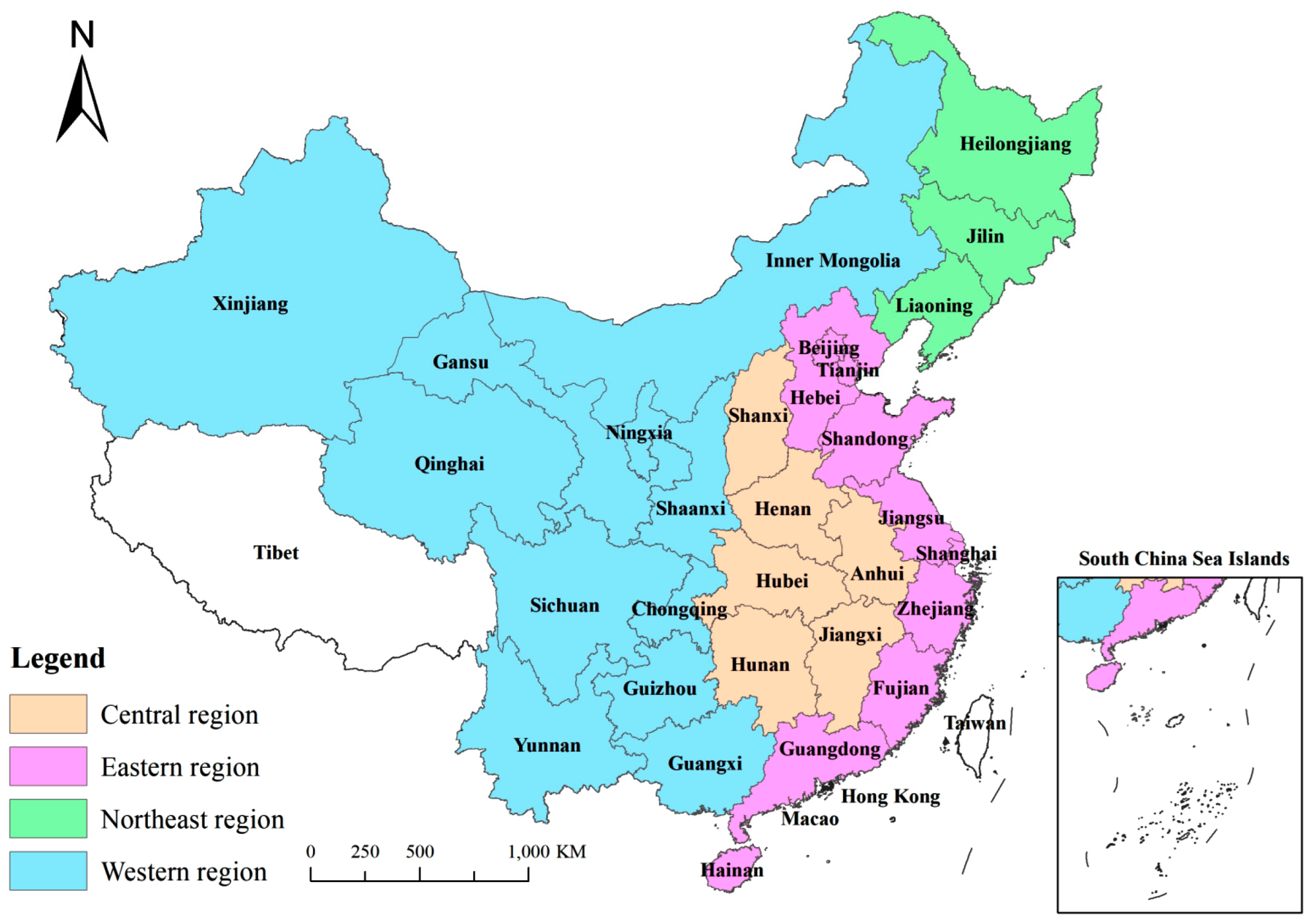
3.1. Research Region and Data Declaration

Considering data availability, 30 provinces in China were delineated as the research region in this paper. Simultaneously, for the purpose of regional heterogeneity analysis, we also separated 30 provinces in China into four major regions according to the divisions of the National Bureau of Statistics: Eastern region, Central region, Western region, and Northeast region (Figure 2).

The data used in this paper were sourced from the National Bureau of Statistics of China (https://www.stats.gov.cn/), China Rural Statistical Yearbook, and provincial statistical yearbooks. Additionally, the data involved in the degree of RDIG were gathered from the China Tertiary Industry Statistical Yearbook, Alibaba Research Institute report, China Economic Net statistical database, Peking University Digital Inclusive Finance Index (2011–2022), and official websites of departments such as the Ministry of Agriculture and Rural Affairs, National Development and Reform Commission.

Linear interpolation and neighboring means were employed to address missing data. To exclude the interference of prices, the total amount of money invested in agricultural fixed assets and the total value of agricultural output were deflated using 2010 as the base period.

3.2. Methodology

3.2.1. Super-Efficient Non-Expected Output SBM-ML Model

The traditional DEA model has several limitations, including, first, the inability to accurately measure efficiency in the presence of undesirable outputs. Second, it is not possible to make further comparisons of effective decision units with efficiency values of 1. Third, the slackness of input and output variables is not considered [25]. Simultaneously, taking into account the green development assertions of non-desired output drop and desired output rise, this paper constructed a global Malmquist–Luenberger productivity index to measure ACEE, which contains undesired outputs by using the relaxation variable model (SBM)-based directional distance function [26]. It can be expressed as:

$${GML}_{\mathrm{t},t+1}=\frac{1+S_G\left(x_{it},y_{it},z_{it};g_x,g_y,g_z\right)}{1+S_G\left(x_{i(t+1)},y_{i(t+1)},z_{i(t+1)};g_x,g_y,g_z\right)}={GEC}_{\mathrm{t},t+1}\times {GTC}_{\mathrm{t},t+1}$$

(1)

where GML denotes the index of ACEE; S_G is the SBM directional distance function with variable returns to scale; x, y, and z are the inputs, desired outputs, and non-desired outputs, respectively; g_x, g_y, and g_z represent the corresponding changes.

Meanwhile, ${GML}_{\mathrm{t},t+1}$ can be decomposed into the product of the technical efficiency index (${GEC}_{\mathrm{t},t+1}$) and the technical progress index (${GTC}_{\mathrm{t},t+1}$).

$${GEC}_{\mathrm{t},t+1}=\frac{1+S_t\left(x_t,y_t,z_t;g\right)}{1+S_{t+1}\left(x_{t+1},y_{t+1},z_{t+1};g\right)}$$

(2)

$${GTC}_{\mathrm{t},t+1}=\frac{1+S_G\left(x_t,y_t,z_t;g\right)}{1+S_t\left(x_t,y_t,z_t;g\right)}\times \frac{1+S_{t+1}\left(x_{t+1},y_{t+1},z_{t+1};g\right)}{1+S_G\left(x_{t+1},y_{t+1},z_{t+1};g\right)}$$

(3)

3.2.2. The Entropy Method

The entropy method, as an objective assignment method, is commonly used in the comprehensive evaluation of multiple indicators. The principle is to determine the weights based on the size of the indicator data, and the greater the weight, the greater the influence on the evaluation system. Compared with other methods, it can eliminate subjective and artificial interference, objectively reflect the information of the original data itself, and make the measurement results more scientific and reasonable. It can be expressed as follows:

(1) Standardized processing

As the units and attributes of the indicators are different, the data need to be standardized to eliminate the effect of the scale. It should be noted that the larger the positive indicator, the better, and the smaller the negative indicator, the better.

$$X_{ij}=\frac{x_{ij}-\min (x_{ij})}{\max (x_{ij})-\min (x_{ij})}$$

(4)

$$x_{ij}=\frac{\max (x_{ij})-x_{ij}}{\max (x_{ij})-\min (x_{ij})}$$

(5)

where x_ij represents the raw value of the jth-indicator in the ith-region; and X_ij is the result after standardization. Formulas (4) and (5) are used to calculate the positive and negative indicators, respectively.

(2) The normalization matrix P

$$P_{ij}=\frac{X_{ij}}{\left({\displaystyle \sum _{i=1}^n{X}_{ij}}\right)}$$

(6)

(3) Entropy value and information entropy redundancy of the jth-indicator

$$e_j=-\frac{1}{\ln (n)}{\displaystyle \sum _{i=1}^n{P}_{ij}\ln (P_{ij})}$$

(7)

$$d_j=1-e_j$$

(8)

(4) The weight of the jth-indicator

$$w_j=\frac{\left(1-d_j\right)}{\left({\displaystyle \sum _{j=1}^m{d}_j}\right)}$$

(9)

(5) The degree of RDIG in the ith-region

$${RDIG}_i={\displaystyle \sum _{j=1}^m{w}_j{P}_{ij}}$$

(10)

3.2.3. Coupling Coordination Model

The degree of coupling coordination is an indicator used to measure the synergistic effect and the degree of synergy between systems. In order to scientifically investigate the degree of coordination between the degree of RDIG (x₁) and ACEE (x₂) in the development process, a coupled coordination model was introduced [27].

$$C=\sqrt[2]{x_1\times x_2}/\left(x_1+x_2\right)$$

(11)

$$T=\alpha x_1+\beta x_2$$

(12)

$$D=\sqrt{C\times T}$$

(13)

where C is the coupling degree, D is the degree of coordination, and T is the comprehensive development index, which is derived by adding the two variables with equal weights. That is, α = β = 0.5. This is because in the coupling and coordinated development process, the two systems are equally important.

Additionally, to ensure comparability, in this paper, x₁ and x₂ were normalized by the polar deviation to make T ∈ [0, 1], which in turn controls D ∈ [0, 1]. In general, there are ten different forms of D [28] (

Table 1. Classification criteria and types of coupling coordination degree.

Coupling Coordination Degree	Coordination Type	Level	Coupling Coordination Degree	Coordination Type	Level
0.000~0.100	Extreme disorder	I	0.500~0.600	Barely coordinated	VI
0.100~0.200	Severe disorder	II	0.600~0.700	Primary coordination	VII
0.200~0.300	Moderate disorder	III	0.700~0.800	Mid-level coordination	VIII
0.300~0.400	Mild disorder	IV	0.800~0.900	Good coordination	IX
0.400~0.500	Near disorder	V	0.900~1.000	High-level coordination	X

).

3.2.4. Spatial Econometric Model

The influencing factors of the coupled coordination degree of RDIG and ACEE in different areas have some degree of spatial correlation because of the input–output correlation and the knowledge spillover effect. Linear regression analysis may not adequately address spatial dependence issues, which can be effectively tackled using spatial econometric models [29]. The commonly used spatial econometric models include the spatial lag model (SAR), spatial error model (SEM), and spatial Durbin model (SDM). Among them, the SDM is more frequently applied to investigate the spatial correlation of geographical units, offering a more comprehensive framework than an SAR or SEM as it contains both the independent and dependent variables’ spatial dependence effects [28].

$$Y_{it}=\rho {\displaystyle \sum _{j=1}^n{W}_{ij}{Y}_{jt}+\delta X_{it}+\phi }{\displaystyle \sum _{j=1}^n{W}_{ij}{X}_{jt}}+{\mu }_i+{\nu }_t+{\epsilon }_{it}$$

(14)

where Y_it is the coupled coordination of RDIG and ACEE; X_it is the influencing factor. ρ is the spatial regression coefficient; W_ij is the normalized spatial weight matrix; and φ represents the spatial correlation error coefficient. μ_i and ν_t represent spatial and temporal effects, respectively; and ε_it is the random error term.

3.3. Establishment of an Indicator System

3.3.1. Indicator System for Measuring ACEE

Based on relevant studies, the four aspects of capital, land, labor, and agricultural resources were used to generate the input indicators, while the desired and non-desired outputs were included in the outputs for measuring ACEE (

Table 2. Indicator system for measuring ACEE.

Indicator Type	First-Level Indicator	Second-Level Indicator	Unit
Input indicators	Capital	Investment stock in agricultural fixed assets	108 yuan
	Land	Total sown area of crops	103 hm2
	Labor	Agricultural employees	104 people
	Agricultural resources	Application amount of fertilizer	104 t
		Application amount of pesticide	t
		Application amount of agricultural film	t
		Total power of agricultural machinery	104 kW
		Effective irrigation area	103 hm2
Output indicators	Economic output	Agricultural total output	108 yuan
	Ecological output	Agricultural carbon sinks	104 t
	Unexpected output	Agricultural carbon emissions	104 t

).

(1) Input indicators

① Capital: Expressed as investment stock in agricultural fixed assets. Since the investment in agricultural fixed assets is a flow indicator in the statistical data, the perpetual inventory method was followed [30], and the investment in agricultural fixed assets in the strict sense was selected. The calculation formula is:

$$K_i^t=\left(1-\rho \right)K_i^{t-1}+I_i^t$$

(15)

where K is the capital stock; ρ is the capital depreciation rate; and I is the investment amount.

② Land: The total sown area of crops was used as a measure, taking into account differences in the replanting index and the effect of the existence of fallow periods in some areas [31].

③ Labor: Represented as agricultural employees. Since data on agricultural employees are not directly available, this paper referred to Tan’s approach and estimated them by using the number of employees in agriculture, forestry, livestock, and fisheries × (total agricultural output value/total agricultural, forestry, livestock, and fisheries output value) [32].

④ Agricultural resources: In light of the current situation of general agricultural production, agricultural resources were examined in five areas: fertilizer, pesticides, agricultural film, agricultural machinery, and irrigation.

(2) Output indicators

① Expected output: Characterized by economic output (total agricultural output) and ecological output (agricultural carbon sinks). Among them, agricultural carbon sinks took into account carbon sequestration during the whole life cycle of the growth of major crops, which was calculated by the formula:

$$C={\displaystyle \sum _{i=1}^n{C}_i}\times Q_i\times \left(1-w\right)/{\lambda }_i$$

(16)

where C represents the total agricultural carbon sink; C_i is the carbon absorption rate per unit of crop; Q_i represents the crop economic yield; w is the water content; and λ_i denotes the crop economic coefficient [3] (

Table 3. Carbon uptake rate, economic coefficient and water content of major crops.

Variety	Economic Coefficient	Water Content	Carbon Uptake Rate	Variety	Economic Coefficient	Water Content	Carbon Uptake Rate
Rice	0.45	12	0.414	Potato	0.70	70	0.423
Wheat	0.40	12	0.485	Sugar cane	0.50	50	0.450
Corn	0.40	13	0.471	Beet	0.70	75	0.407
Legume	0.34	13	0.450	Vegetable	0.60	90	0.450
Rapeseed	0.25	10	0.450	Melon	0.70	90	0.450
Peanut	0.43	10	0.450	Tobacco	0.55	85	0.450
Sunflower	0.30	10	0.450	Other	0.40	12	0.450
Cotton	0.10	8	0.450

).

② Unexpected output: Characterized by agricultural carbon emissions. It includes emissions from implicit carbon sources of agricultural chemical inputs (e.g., fertilizer, pesticides, films) and carbon sources stemming from agricultural activities (e.g., machinery, plowing, and irrigation).

$$E={\displaystyle \sum _{i=1}^n{E}_k=}{\displaystyle \sum _{i=1}^n{T}_k\times {\delta }_k}$$

(17)

where E is agricultural carbon emissions; E_k is the kth-carbon source’s total carbon emissions; T_k is its absolute amount; and δ_k is its carbon emission coefficient, which is as follows: fertilizer (0.896 kg·kg⁻¹), pesticide (4.934 kg·kg⁻¹), film (5.180 kg·kg⁻¹), agricultural diesel (0.593 kg·kg⁻¹), plowing (312.600 kg·km⁻²), and irrigation (25.000 kg·km⁻²) [33].

3.3.2. Indicator System for the Development of RDIG

Based on relevant research [34], we selected 15 indicators to construct the index system from three aspects: digital infrastructure, rural digital industrialization, and rural industrial digitization (

Table 4. Index system for the development of RDIG.

Guideline Layer	Indicator Layer	Calculation Method (Attribute)	Unit
Digital infrastructure	Rural Internet penetration rate (X1)	Users of broadband connectivity in rural areas as a percentage of all rural users (+)	%
	Rural mobile phone penetration rate (X2)	Per 100 rural families, the average number of mobile phones owned (+)	a
	Rural computer penetration rate (X3)	Average computer ownership per hundred rural households (+)	a
	Broadcasting and television network coverage (X4)	Number of rural cable broadcasting and television/total number of rural households (+)	%
	Number of agricultural meteorological observation stations (X5)	The quantity of weather observation stations for agriculture (+)	a
Rural digital industrialization	Number of rural digital bases (X6)	Number of Taobao villages (+)	a
	Consumer level of digital products and services (X7)	Rural Engel’s coefficient (−)	%
	The quantity and scale of rural online payments (X8)	Rural digital inclusive finance index (the mean of different county-level indices in the Peking University Digital Inclusive Finance Index reflects the quantity and scale of rural online payments) (+)	/
	National Modern Agriculture Demonstration Project (X9)	Number of national key leading enterprises in agricultural industrialization (+)	a
Rural industrial digitization	Scale of agricultural digitization (X10)	Digital activities’ added value in the primary industry (we used an input–output table data to obtain the digital economy adjustment coefficient of the primary industry, i.e., the ratio of intermediate investment in digital products and services in the primary industry to the total intermediate investment in the primary industry. The added value of digital activities in the primary industry was calculated as the digital economic adjustment coefficient of the primary industry multiplied by the added value of the primary industry) (+)	108 yuan
	Digital trading of agricultural products (X11)	Agriculture-related products sold in retail online (the “online retail sales of physical goods” measures the degree of digital trading of agricultural products) (+)	108 yuan
	Service scope of information technology applications such as the Internet of Things (X12)	Route length for rural deliveries (+)	km
	Postal communication service level (X13)	Average weekly delivery frequency in rural areas (+)	a
	Digital service consumption level (X14)	Per capita transportation and communication consumption expenditure of rural households (+)	yuan
	Digital service talent team (X15)	Number of agricultural technicians (+)	104 people

). Finally, the entropy method was used to assign weights to each indicator, so as to find out the degree of RDIG in each province.

4. Spatial-Temporal Differences of Coupling Coordination

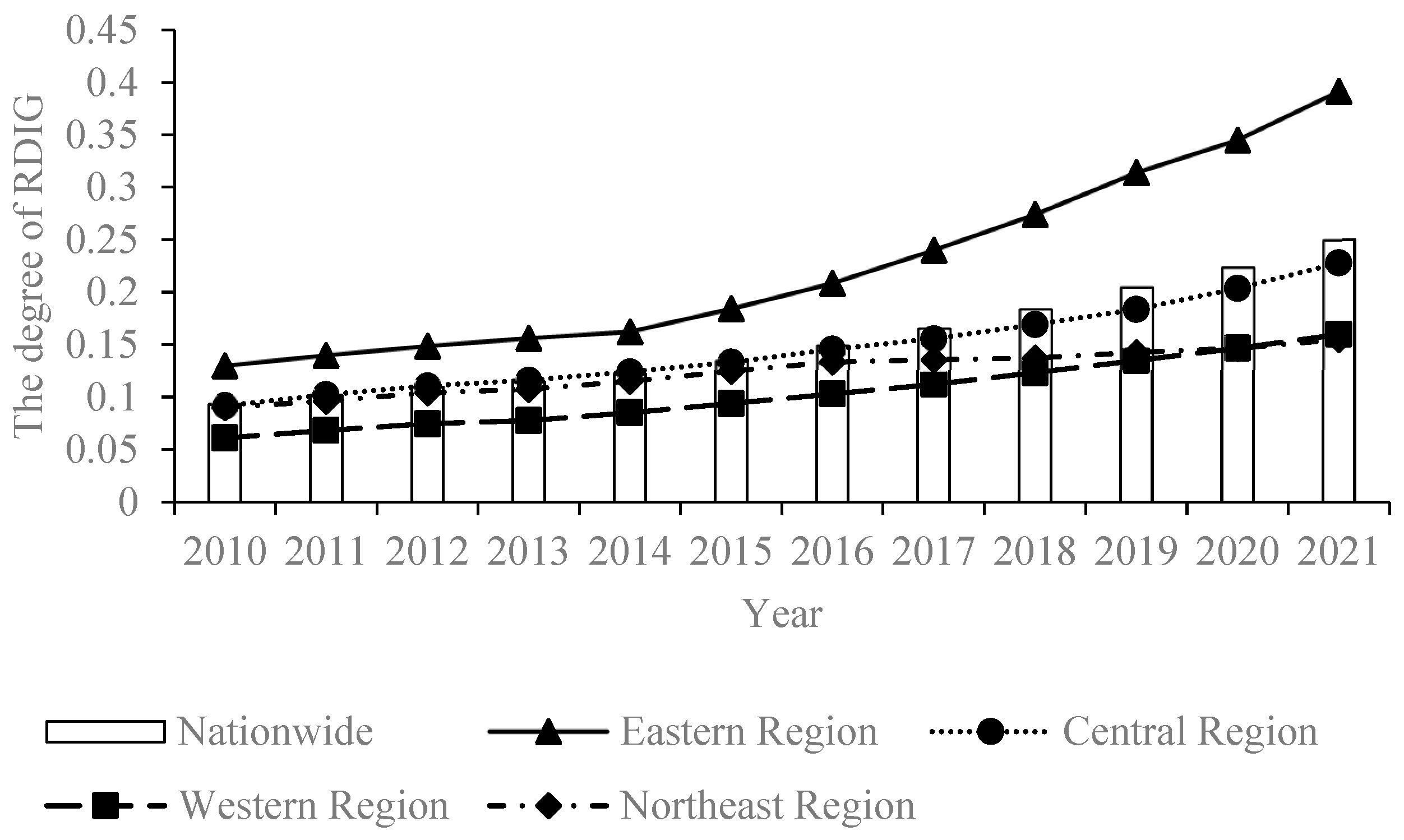
4.1. Spatial-Temporal Features of the Degree of RDIG

(1) The degree of RDIG is increasing in the temporal dimension, both nationally and at the level of the four regions (Figure 3). Specifically, the average value of China’s degree of RDIG at the beginning of the period is 0.093, and the average value at the end of the period is 0.250, exhibiting a 9.41% average yearly growth rate, which shows that the transformation of RDIG is highly effective. Regionally, the Eastern region has the greatest degree of RDIG, with a mean value of 0.225 and an average annual growth rate of 10.55%. The Central and Northeastern regions are next in line, with mean values of 0.147 and 0.124, correspondingly, and yearly growth rates of 8.61% and 5.06% on average. The Western region has the lowest level of RDIG, with a mean value of 0.103 and an average annual growth rate of 9.11%. As a result, there is still a long way to go to deepen the degree of RDIG, and the average annual growth rate in the Western region is second only to that in the East, with a “catching-up effect” thanks to the tilting of national policies in recent years and the support of the Eastern region.

(2) In the spatial dimension, whether in the four regions or in each province, the unevenness of the rural digital space is obvious, and the problem of the regional “digital divide” is serious. Regionally, the degree of RDIG shows a “stepped” spatial distribution pattern of decreasing from the Eastern coastal areas to the Western inland areas, with significant regional differences. This is consistent with the results of the “County Digital Rural Index Research Report (2020)” released by the Digital Rural Project Team of the Institute of New Rural Development of Peking University [34]. The geographical location, resource endowment, and economic level of the Eastern region are better than those of the other regions, and there are realistic conditions for “promoting agriculture with industry and bringing the rural to the city”, and the RDIG is gradually deepening. In contrast, the Central–West and Northeastern regions lack a strong impetus for development due to the weak digital infrastructure and lack of development funds. Therefore, there is still a need to follow up on such strategies as the development of the Western region, the rise of the Central region, and the revitalization of the Northeastern region, as well as precise regional support, so as to achieve coordinated regional development. For the provinces, Zhejiang, Guangdong, Jiangsu, Shandong, and Fujian rank among the top five in China when it comes to RDIG. They are all in the Eastern region, with measured means of 0.381, 0.351, 0.319, 0.271, and 0.216, respectively (

Table 5. RDIG and decomposition results of ACEE.

Area	Province	RDIG	ML	EC	TC	Area	Province	RDIG	ML	EC	TC
Eastern Region	Beijing	0.191	1.050	0.956	1.098	Western Region	Inner Mongolia	0.107	1.067	0.998	1.069
	Tianjin	0.098	1.099	1.012	1.086		Guangxi	0.121	1.002	0.994	1.008
	Hebei	0.197	1.056	1.005	1.051		Chongqing	0.094	1.081	1.004	1.077
	Shanghai	0.144	1.021	0.987	1.034		Sichuan	0.171	1.055	0.997	1.058
	Jiangsu	0.319	1.034	0.996	1.038		Guizhou	0.091	1.029	1.010	1.019
	Zhejiang	0.381	1.061	0.973	1.090		Yunnan	0.101	1.071	1.046	1.024
	Fujian	0.216	1.090	1.001	1.089		Shaanxi	0.128	1.060	0.993	1.067
	Shandong	0.271	1.042	0.982	1.061		Gansu	0.094	1.057	1.015	1.041
	Guangdong	0.351	1.060	1.003	1.057		Qinghai	0.059	1.184	1.043	1.135
	Hainan	0.079	1.058	1.004	1.054		Ningxia	0.066	1.082	0.998	1.084
	Average	0.225	1.057	0.992	1.066		Xinjiang	0.106	1.013	1.002	1.011
Central Region	Shanxi	0.106	1.042	0.999	1.043		Average	0.103	1.063	1.009	1.054
	Anhui	0.149	1.028	1.010	1.018	Northeast Region	Liaoning	0.130	1.066	1.025	1.040
	Jiangxi	0.125	1.038	1.016	1.022		Jilin	0.113	1.047	1.006	1.041
	Henan	0.176	1.033	0.997	1.036		Heilongjiang	0.129	1.038	1.014	1.024
	Hubei	0.180	1.064	1.002	1.062		Average	0.124	1.051	1.015	1.035
	Hunan	0.146	1.025	0.977	1.049	Average		0.150	1.052	1.004	1.048
	Average	0.147	1.038	1.000	1.038

Note: ML = EC × TC, where ML refers to ACEE, EC represents technological efficiency, and TC represents technological advancement.

). This is because the Eastern region, as a “pioneer zone” for opening up and a “testing ground” for reform, often comes out on top in terms of the economic growth rate, and its quickly expanding financial investment offers robust assistance for rural areas’ digital transformation. However, the average values of RDIG in Qinghai, Ningxia, and Guizhou are all lower than the national average and rank relatively low. This indicates that there is still much room for improvement, which can be attributed to the remote location and backward level of economic development in the Western region.

4.2. Spatial-Temporal Features of ACEE

(1) In the time dimension, from 2010 to 2021, China’s ACEE as a whole shows an “N-shaped” change, that is, it first rises, then falls, and finally, rises voluntarily (Figure 4). In detail, the ACEE shows an increase between 2010 and 2011. From 2011 to 2017, there is a downward trend, reaching a trough in 2017. This is due to the strong burden on the environment caused by China’s long-standing “rough” production methods, which have invested heavily in agricultural chemicals and relied excessively on agricultural machinery and energy. Accordingly, the General Offices of the Central Committee of the CPC and the State Council released the “Opinions on Innovative Institutional Mechanisms to Promote Green Agricultural Development” in 2017 [34]. This initiative underscores the cyclic and low-carbon development of agriculture, and it creates a methodical framework for agriculture’s transition to a more ecological and green industry. Over the period 2017–2021, ACEE achieves a significant increase of about 17.9% per year.

As far as internal decomposition is concerned, the trend of China’s ACEE is co-determined by technological efficiency and technological advancement. This trend is highly similar to that of technical progress. In other words, the development of agricultural production technology is primarily responsible for China’s increase in ACEE over the research period. Nevertheless, the technical efficiency of agricultural production has shown a fluctuating and slightly decreasing trend, and its contribution to ACEE has been insufficient. This suggests that there is still much room for improvement in the current rationing of input resources and equipment efficiency in agricultural production.

(2) In the spatial dimension, whether in the four regions or in each province, the ACEE is differentiated and regionalized. Regionally, the overall spatial distribution pattern of ACEE is “high in the West, followed by the East and Northeast, and low in the Middle”, with obvious regional differences. The improvement of ACEE in the Western region is mainly due to the strategy of “Western Development”. With the adjustment of the agricultural structure and the inflow of capital and technology under this strategy, the Western region vigorously develops characteristic agriculture by virtue of its advantages in terms of natural resources and actively realizes the construction of modern agriculture, thus continuously improving the technical level and efficiency of agricultural production. For the provinces, Qinghai, Tianjin, Fujian, Ningxia, and Chongqing rank among the top five in China, mainly in the Eastern and Western regions (Table 5). While Guangxi, Xinjiang, and Shanghai rank relatively low, their ACEE is below the average for the country. Looking at the internal decomposition of each province, 17 provinces belong to a “dual-driven” growth model, which is characterized by both technological advancement and increased technical efficiency. The remaining 13 provinces, conversely, embrace a “single-driver” growth model that depends on advancements in technology at the expense of technical efficiency. Although these provinces have made significant strides in implementing new technologies, the application of current technologies has not kept up with the expansion of production frontiers, which has led to a sluggish increase in ACEE.

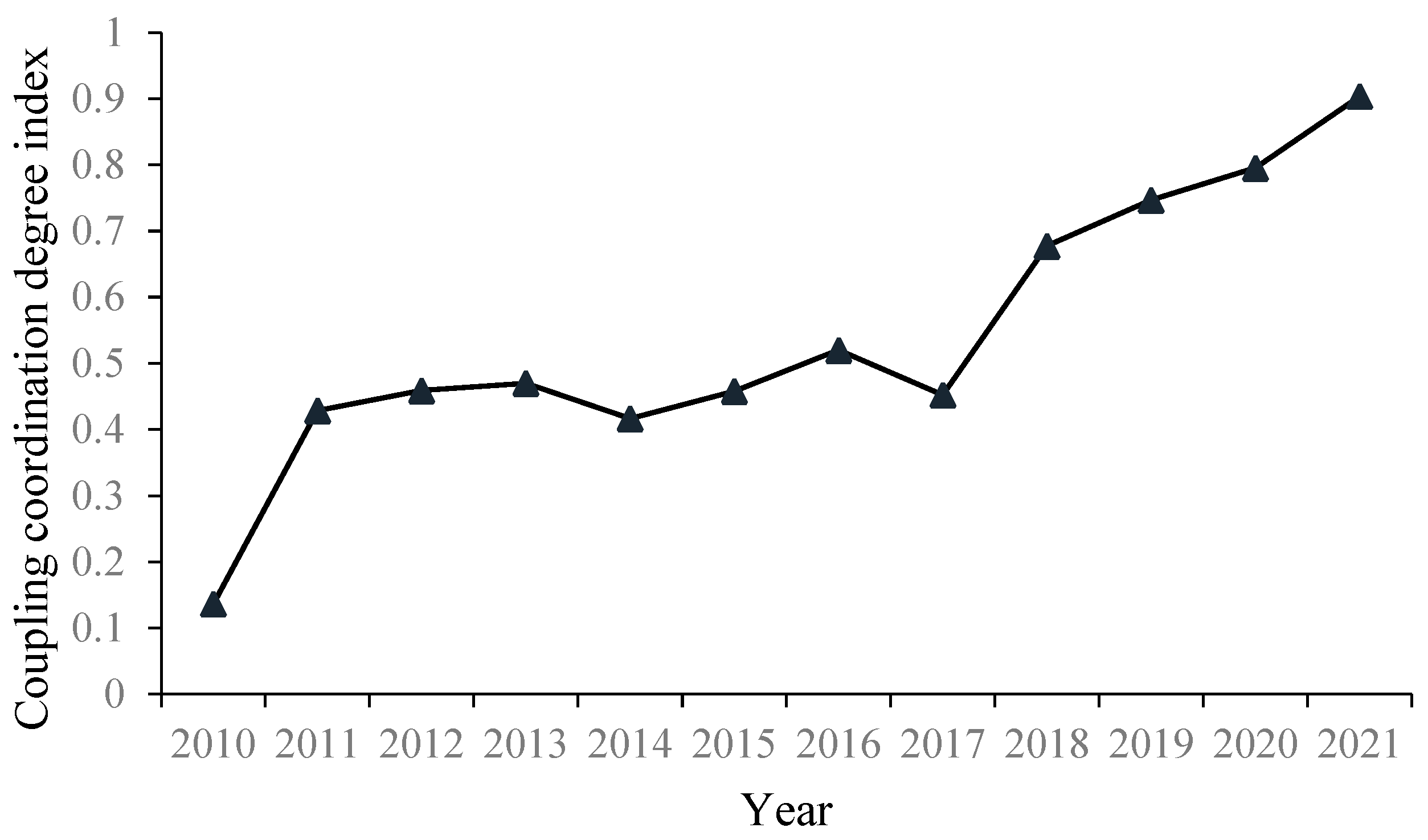
4.3. Spatial-Temporal Features of Coupling Coordination

(1) In terms of the temporal features, the coupling coordination in China shows a fluctuating growth process overall from 2010 to 2021. Specifically, it rises from 0.137 to 0.904, exhibiting an annual growth rate averaging as high as 18.73%, and rising from “extreme disorder” to “high-level coordination” (Figure 5). The coupling coordination index shows a slight decrease from 2013 to 2014 and from 2016 to 2017. The former coordination type remains “near disorder”, while the latter decreases from “barely coordinated” to “near disorder”. This shows that with the development of the digital economy and the dissemination of the concept of green low-carbon, the coupling coordination of the two as a whole is improving, but we still need to adopt targeted measures to improve and regulate.

(2) In terms of the spatial features, the coupled coordination between the degree of RDIG and ACEE shows obvious spatial characteristics. Regionally, the average values of the coupling coordination in 2010, from high to low, are the Northeast (0.170), Eastern (0.156), Central (0.137), and Western region (0.110). In 2021, the ranking is the Eastern (0.911), Western (0.907), Northeastern (0.899), and Central region (0.888) (

Table 6. Coupling coordination degree index and type in China.

Area	Province	2010	Level	2021	Level	Area	Province	2010	Level	2021	Level
Eastern Region	Beijing	0.155	II	0.999	X	Western Region	Inner Mongolia	0.137	II	0.531	VI
	Tianjin	0.153	II	1.000	X		Guangxi	0.032	I	0.970	X
	Hebei	0.169	II	0.911	X		Chongqing	0.115	II	0.942	X
	Shanghai	0.191	II	0.887	IX		Sichuan	0.139	II	1.000	X
	Jiangsu	0.136	II	0.685	VII		Guizhou	0.032	I	0.876	IX
	Zhejiang	0.178	II	0.992	X		Yunnan	0.032	I	1.000	X
	Fujian	0.135	II	1.000	X		Shaanxi	0.173	II	0.909	X
	Shandong	0.145	II	1.000	X		Gansu	0.160	II	1.000	X
	Guangdong	0.161	II	0.745	VIII		Qinghai	0.122	II	1.000	X
	Hainan	0.136	II	0.892	IX		Ningxia	0.140	II	0.750	VIII
	Average	0.156	II	0.911	X		Xinjiang	0.131	II	1.000	X
Central Region	Shanxi	0.178	II	0.958	X		Average	0.110	II	0.907	X
	Anhui	0.163	II	0.853	IX	Northeast Region	Liaoning	0.167	II	1.000	X
	Jiangxi	0.032	I	0.734	VIII		Jilin	0.164	II	0.938	X
	Henan	0.137	II	0.834	IX		Heilongjiang	0.178	II	0.758	VIII
	Hubei	0.139	II	1.000	X		Average	0.170	II	0.899	IX
	Hunan	0.175	II	0.948	X	Average		0.143	II	0.901	X
	Average	0.137	II	0.888	IX

). It can be seen that from 2010 to 2021, the four regions’ coupling coordination indexes have achieved different degrees of growth. For the provinces, in 2010, the coupling coordination degree of each province in China ranges from 0.032 to 0.191, all of which are at the stage of “extreme dissonance” and “serious dissonance”, with “serious dissonance” dominating. In 2021, it ranges from 0.531 to 1.000, with a predominance of “high-level coordination” (Figure 6). This indicates that each province has realized a significant increase in coupling coordination, especially Yunnan, Guangxi, and Qinghai. This is mostly because pertinent policies like building digital villages, and promoting green and high-quality development of agriculture have strong support.

5. Influencing Factors and Discussion

5.1. Selection of Influencing Factors

(1) Government input—GI (10⁸ yuan): Expressed as local finance expenditure on agriculture, forestry, and water affairs. Government financing and regulation are needed for rural digital development. Moreover, ACEE cannot be improved without the administrative functions of the government. However, government inputs may distort the structure of factor inputs and stimulate farmers to increase chemical inputs [35], which in turn is detrimental to ACEE.

(2) Educational level—EL (year): Expressed as the average years of education. The digital development of rural areas is driven by technological innovation and has a certain threshold requirement for the level of education. Increased levels of education can promote continuous innovation in agricultural technology, which in turn affects ACEE. For example, advances in agricultural pollution management technologies can reduce the pollution emissions generated by agricultural production factors, thereby enhancing ACEE [36].

(3) Industrial structure—IS (%): Denoted by the proportion of the total value of agricultural production to the combined value of agricultural, forestry, livestock, and fisheries output. The industrial structure holds the potential for the digitalization of production and consumption, which affects the demand and layout of different types of digital infrastructure. However, China’s “extensive production mode” has not been fundamentally reversed and agricultural cultivation in many regions still relies on high inputs of chemical fertilizers and pesticides [37], which is detrimental to agricultural carbon reduction.

(4) Energy use—EU (kW·h): Expressed by rural electricity consumption. Agricultural development relies on infrastructure such as rural electricity grids, especially for irrigation operations. Although electricity consumption generates carbon emissions, compared with the carbon emissions resulting from energy consumption, the former is significantly less. Therefore, rural electricity consumption contributes, to some extent, to ACEE.

(5) Urbanization rate—UR (%): Expressed by the proportion of the total population living in urban areas. The development of new urbanization needs the support of digital infrastructure, especially the construction of smart cities, which is rather inseparable from digital technology [38]. With the increase in urbanization rates, agricultural infrastructure development has proliferated in the short term, which has resulted in a marked increase in the use of resources in rural areas, contamination of the environment, and carbon emissions from agriculture [39].

(6) Living standards—LS (yuan): Expressed as the per capita disposable income of rural residents. The digital transformation of rural areas can boost entrepreneurial activity and the scale of non-farm employment, thus helping farmers increase their income. However, the stimulation of farmers’ entrepreneurial willingness and enthusiasm has in turn led to a low level of attention to agricultural cultivation and a low level of participation in agricultural carbon emission reduction efforts, thus hindering the improvement of ACEE.

5.2. Regression Results

To select an appropriate spatial econometric model, the LM test, the Hausman test, the Wald test, and the LR test were conducted in this paper. The test results revealed that the SDM model with time-fixed effects was the best choice. Therefore, to process the SDM model, an inverse geographic weight matrix was employed.

In

Table 7. Spatial panel regression results.

Variable	SDM	Direct Effect	Indirect Effect	Total Effect	WX	Interaction Effect
GI	−0.071 ** (0.032)	−0.069 ** (0.032)	−0.044 (0.152)	−0.113 (0.155)	W*GI	−0.091 (0.204)
EL	0.072 *** (0.022)	0.074 *** (0.021)	−0.101 (0.116)	−0.027 (0.125)	W*EL	−0.106 (0.177)
IS	−0.113 (0.130)	−0.102 (0.129)	−0.064 (0.835)	−0.166 (0.835)	W*IS	−0.262 (1.180)
EU	0.028 ** (0.013)	0.026 ** (0.013)	0.052 (0.059)	0.078 (0.062)	W*EU	0.083 (0.081)
UR	−0.005 ** (0.002)	−0.005 ** (0.002)	0.025 ** (0.010)	0.019 ** (0.009)	W*UR	0.032 ** (0.014)
LS	−0.155 ** (0.068)	−0.127 * (0.068)	−0.884 ** (0.350)	−1.012 *** (0.346)	W*LS	−1.328 *** (0.461)
μi	Yes
νt	Yes
Rho/λ (Rho/λ reflects the magnitude and direction of the spatial hysteresis effect, with a value between −1 and 1. When Rho/λ is equal to 0, the spatial lag value of each factor has no effect on the degree of coupling coordination; when Rho/λ is positive, the increase of each factor in neighboring regions has a positive effect on the increase of coupling coordination; when Rho/λ is negative, the increase of each factor in neighboring regions has a negative effect on the improvement of coupling coordination)	−0.438 ** (0.219)
sigma2_e (In the regression results of the SDM model, sigma2_e represents the variance of the spatial error term, which is the degree of spatial autocorrelation error. If sigma2_e is small, then the spatial autocorrelation error is small and the SDM model fits well. If sigma2_e is large, then the spatial autocorrelation error is large and the fitting effect of SDM model is poor)	0.021 *** (0.002)
R2	0.422
Log-likelihood	183.380
Moran’s I (The Moran’s I index is commonly used to measure the spatial correlation between variables. Its value range is [−1,1]. A closer value to 1 or −1 indicates a stronger spatial correlation in the sample space. When closer to 0, this index indicates lower spatial autocorrelation among sample enterprises)	17.232 ***
LM-error (Lagrange multiplier (LM) and robust Lagrange multiplier (Robust LM) tests are used to determine the necessity of using spatial econometric models. The LM test passes significance, indicating that there is a certain spatial correlation between the explained variable and the explanatory variable; it was necessary to introduce a spatial econometric model)	253.281 ***
Robust LM-error	11.649 ***
LM-lag	302.512 ***
Robust LM-lag	60.880 ***
Wald-spatial lag	10.86 *
LR-spatial lag (LR and Wald tests are used to diagnose whether the SDM model will be simplified into the SAR model and SEM model. The LR and Wald tests pass significance, indicating that the fitting effect of the SDM was superior to the SAR and SEM in our case)	12.24 *
Wald-spatial error	12.17 *
LR-spatial error	11.68 *
Hausman (The Hausman test is used to determine whether the study applies to fixed or random effects. The Hausman test passes significance, indicating that the null hypothesis should be rejected and fixed effects should be selected)	30.84 ***

Note: *, **, *** denote significant at the 10%, 5%, 1% level respectively. The values in brackets indicate the robust standard error of each coefficient.

, Moran’s I is 17.232 and significant at the 1% level. This suggests a strong spatial dependence of the coupling coordination degree. Thus, the decomposition effect (e.g., direct effect and indirect effect (the direct effect represents the impact of local factors on the local coupling coordination and the indirect effect represents the impact of local factors on the degree of coupling coordination in the neighborhood)) of the SDM must be the main focus, and the marginal effects of each influencing factors must be examined.

In terms of the direct effects, the order of the contribution intensity of each factor is: LS # > EL > GI # > EU > UR # (“#” stands for a negative effect). This suggests that higher levels of both education and energy use are conducive to improving the local coupled coordination. On the contrary, improved living standards, increased government investment, and higher urbanization rates can reduce the local coupling coordination. The order of spatial spillovers is: LS # > UR. This suggests that an increase in the local urbanization rate improves the coupling coordination of neighboring regions, unlike the improvement in the living standards of local rural residents, which has a negative attenuating effect. Furthermore, there are no appreciable geographical spillover effects of the remaining factors on the coupling coordination. Table 7 also shows the coefficient estimates that characterize the exogenous interaction effect (WX). W × UR and W × LS all show relatively high significance.

Additionally, to ensure the accuracy of our findings, a series of tests were conducted in this paper based on replacing the spatial weight matrix (using the 0–1 spatial weight matrix to estimate the SDM model again), quadratic regression on significant variables, and considering the sample selection bias (1% shrinkage of sample data). The findings demonstrate that the model is resilient since the significance of the variables remains relatively constant regardless of the test strategy used.

5.3. Discussion

The above empirical tests find that different influencing factors have different effects on the coupled and coordinated development of the two. The specific analysis is as follows:

(1) The coefficient of GI exhibits statistical significance at the 5% confidence level, displaying a negative value. Increased government investment has provided the necessary financial, technical, and human resources support for the digital transformation of rural areas. However, some officials are limited by performance appraisal and tend to choose “short-frequency and quick” projects, paying too much attention to economic benefits and neglecting the consideration of long-term sustainable development and environmental protection. To a certain extent, this may lead to the irrational structure of capital investment and insufficient ecological subsidies [35]. Since 2004, the government has increased agricultural subsidies for agricultural machinery and fertilizers in order to increase agricultural production capacity. However, this has led to the high use of fertilizers by farmers, thus discouraging carbon emission reduction in agriculture. Simultaneously, “strong government” tends to create a “weak market” [40]. As low-carbon green development in agriculture is not a one-day process and has a high demand for investment, it is necessary to bring the financing capacity of the market into play in order to promote the coordinated development of the RDIG and ACEE.

(2) The coefficient of EL is positively and significantly associated at the 1% significance level. The educational attainment level plays a pivotal role in shaping individuals’ capacity to embrace novel concepts. Increased levels of education can promote innovation in agricultural management, reduce excessive inputs of agrochemicals [41], and enhance the recycling of agricultural waste, thereby improving ACEE. Similar results have been reported in past studies of ACEE. For instance, taking Brazil as the research object, Rada and Buccola (2012) found a positive correlation between education level and technical advancement [42]. Technological developments in agricultural pollution control can lower the amount of pollution that agricultural production factors produce. This can improve the carbon emission efficiency of agriculture [36], thereby achieving good coordination between RDIG and ACEE.

(3) The coefficient of IS demonstrates a lack of statistical significance, with a negative sign. The industrial structure holds the potential for the digitalization of production and consumption, which affects the demand and layout of different types of digital infrastructure [40], and to a certain extent, it can facilitate the digital transformation of rural areas. Compared to forestry, livestock, and fisheries, planting is the most energy-consuming and greenhouse gas-emitting sector of agriculture [32,39]. This is due to the fact that China’s “extensive production mode” has not been fundamentally reversed. Meanwhile, the planting structure adjustment involves the allocation of all kinds of production factors and the optimization and upgrading of production links, which is not achievable in the short term, so it has not yet passed the significance test.

(4) The coefficient of EU exhibits statistical significance at the 5% confidence level with a positive value. The digital transformation of rural areas has a high degree of dependence on energy use. With the gradual transformation of traditional agriculture into modern agriculture, electricity is gradually becoming an alternative energy source to oil. ACEE is enhanced because using electricity for agricultural production results in somewhat fewer greenhouse gas emissions than using oil [32]. This conclusion has been verified in both Chinese and Norwegian agriculture. Specifically, Olkkonen et al. (2023) focused on the development of electrification in the Norwegian agricultural sector, noting that electrification of on-field tractor operations can reduce CO₂ emissions in the agricultural sector related to tractor energy use in order to phase out fossil fuels [43]. Jin et al. (2024) focused on the unidirectional driving effect of the rural digital economy on the intensity of agricultural carbon emissions in the case of China and similarly argued that electricity consumption instead of energy consumption reduced agricultural carbon emissions to some extent [44]. The degree to which digital infrastructure is being adopted in rural areas is also reflected in the rise in electricity consumption in these locations. Strong facilities for the digital transformation and modernization of rural areas are provided by the robust improvement of the digital infrastructure, which influences the coupled and coordinated development.

(5) The coefficient of UR demonstrates statistical significance at the 5% level with a negative value. The construction of new urbanization, as a key part of the Chinese-style modernization process, is increasingly dependent on digital infrastructure. This dependence provides a wide range of application scenarios and market demand for the development of digital technology, thus promoting the innovation and application of digital technology. However, in turn, urbanization poses a serious challenge to agricultural carbon reduction. Specifically, the increased rate of urbanization has provided opportunities for industrial and manufacturing development, thus promoting the production and application of agricultural machinery, electrification facilities, and agricultural chemicals. Numerous academics have also verified this finding [9,39]. That is to say, the urbanization rate can constrain coordinated development.

(6) The coefficient of LS is statistically significant at the 5% level with a negative value. According to statistics, wage income accounts for more than 40% of the rise in rural residents’ income. This is due to the fact that the digital transformation of rural areas can boost entrepreneurial activity and the scale of non-farm employment, thereby helping farmers increase their income. The strengthening of digital infrastructure and the use of digital technologies have surely benefited financially from the increase in rural residents’ income. This initiative can help the digital transformation and upgrading of rural areas, giving rise to new forms and modes of agricultural economic development, such as rural tourism, leisure farms, and live streaming of goods. It not only expands the market for the sale of agricultural products but also stimulates the entrepreneurial willingness and enthusiasm of farmers [45]. However, this kind of non-farm employment and entrepreneurship makes the majority of rural residents pay little attention to agricultural cultivation and naturally have little participation in the work of agricultural carbon emission reduction, thus hindering the improvement of ACEE.

(7) The findings of the spillover study suggest that the cross-regional effects of variables like the rate of urbanization and living standards should be taken into account when developing regional policies to support the coordinated growth of RDIG and ACEE. All the provinces and regions should be taken into consideration when designing policies for coordinated national development.

6. Conclusions and Implications

6.1. Conclusions

To fulfill the “dual-carbon” goal and quicken the low-carbon and environmentally friendly development, taking 30 provinces (autonomous regions and municipalities) as the research object, the coupling coordination level and the spatial-temporal evolution features were investigated and the influencing factors were thoroughly examined in this paper based on the clarification of the degree of RDIG and ACEE. The results are summarized as follows:

(1) In terms of the degree of RDIG, the overall trend has been gradually increasing from 0.093 to 0.250, exhibiting a 9.41% average yearly growth rate. It is evident that rural areas are effectively undergoing a digital transformation. The degree of spatial imbalance is obvious, and there is a “stepped” spatial distribution pattern of decreasing from the Eastern coastal areas to the Western inland areas. In terms of ACEE, there is an overall “N-shaped” change. This change is determined by a combination of technical advancement and efficiency, with the former playing a dominant role. Regionalization and differentiation are notable, with regional annual averages for, in descending order, the Western, Eastern, Northeastern, and Central regions.

(2) From 2010 to 2021, the coupling coordination index increases in fluctuation from “extreme disorder” to “high-level coordination”. Furthermore, there are distinct regional differences in the degree of coupling coordination in various places. In other words, the coupling coordination indexes of the four major regions have all achieved varying degrees of growth, in descending order: the Western, Eastern, Central, and Northeastern areas. Greater attention ought to be paid to areas with low coupling coordination.

(3) The coupling coordination is jointly influenced by a variety of factors. Educational level and energy use both significantly and favorably affect the coupling coordination. Government input, urbanization rate, and living standards have negative and significant effects, whereas the significant impact of industrial structure is unclear.

6.2. Implications

To better support the coordinated development of “green mountains” and “silver mountains” (“Green mountains” are as good as “silver mountains”, that is, improving the ecological environment is key to developing productivity) and to achieve the “dual-carbon” goal, the following implications are put forward.

(1) A system’s ability to transition from disorder to order and achieve coordinated development is largely dependent on the “synergetic effect” between its internal subsystems. This synergy shapes the character and pattern of the system’s phase transitions. This research shows that the magnitude of the coupling coordination degree reflects the degree of coordination between RDIG and ACEE. The digital transformation of rural areas can effectively maintain green functions by reducing resource wastage in agricultural production and lowering the cost of agricultural operations. The digital transformation and upgrading of rural areas are made possible by ACEE, which also has a feedback-driven impact on them. A key metric for determining whether or not the two have successfully achieved efficient synergy is the coupling coordination degree.

(2) During this crucial time for promoting the all-encompassing revitalization of rural areas and the development of an ecological society, it is crucial to achieve “win-win” coordinated development for the digital transformation of rural areas and ACEE. This development necessitates localizing regional policies, in addition to innovative common system design at the highest level. It is desirable to provide a better policy environment for the digital transformation of rural areas and the low-carbon and environmentally friendly development of agriculture. Within the region, attention should be paid to the negative effects of improved living standards and rapid urbanization on the coordinated development. Non-farm entrepreneurial employment and environmental governance pressures from urbanization should be scientifically channeled. The rational use of renewable energy sources, such as biomass, can be realized by attracting technology and talent, thus contributing to low-carbon agricultural development. At the interregional level, cross-regional exchanges and cooperation are being promoted. Regional synergistic governance and balanced development can be achieved by encouraging lagging regions to actively take advantage of the spillover effects of urbanization in neighboring regions on their own digital transformation and low-carbon green development in agriculture. For example, for the Eastern region, which has a higher level of economic development, advanced experiences should be vigorously promoted. The Western region, where the level of economic development and rural digitization is relatively low, should pay attention to the exchange and cooperation of agricultural technology, learn and absorb advanced management systems, and explore diversified agricultural carbon emission reduction paths, so as to help achieve the “dual-carbon” goal.

(3) Like all studies, this one has limitations. Considerable socioeconomic variations exist among counties within provinces. Accessing comprehensive and viable county-level data through field investigations and interviews, or undertaking comparative analyses of different county-level development cases, could enhance the accuracy and depth of research on the coupling and coordination degree between the degree of RDIG and ACEE. This is a direction that needs to be improved and refined in the future. Nevertheless, this paper has studied the spatial differences between the degree of RDIG and ACEE in China at the national and provincial levels, grasped the influencing factors concerning the degree of coordination between the two from a macroscopic point of view as a whole, and produced robust and detailed empirical results, which have laid a certain foundation for deepening the relevant research.

References

1. Johnson, J.M.F.; Franzluebbers, A.J.; Weyers, S.L.; Reicosky, D.C. Agricultural opportunities to mitigate greenhouse gas emissions. Environ. Pollut. 2007, 150, 107–124. [Google Scholar] [CrossRef] [PubMed]
2. Cui, Y.; Khan, S.U.; Sauer, J.; Zhao, M.J. Exploring the spatiotemporal heterogeneity and influencing factors of agricultural carbon footprint and carbon footprint intensity: Embodying carbon sink effect. Sci. Total Environ. 2022, 846, 157507. [Google Scholar] [CrossRef] [PubMed]
3. Tian, Y.; Zhang, J.B. Regional differentiation research on net carbon effect of agricultural production in China. J. Nat. Resour. 2013, 28, 1298–1309. [Google Scholar]
4. Kaya, Y.; Yokobori, K. Environment, Energy, and Economic: Strategies for Sustainability; United Nations University Press: Tokyo, Japan, 1997. [Google Scholar]
5. Guo, X.J.; Wang, X.; Wu, X.L.; Chen, X.P.; Li, Y. Carbon emission efficiency and low–carbon optimization in Shanxi Province under “dual carbon” background. Energies 2022, 15, 2369. [Google Scholar] [CrossRef]
6. Zhou, P.; Ang, B.W.; Han, J.Y. Total factor carbon emission performance: A Malmquist index analysis. Energy Econ. 2010, 32, 194–201. [Google Scholar] [CrossRef]
7. Wu, H.Y.; Huang, H.J.; Chen, W.K.; Meng, Y. Estimation and spatiotemporal analysis of the carbon–emission efficiency of crop production in China. J. Clean. Prod. 2022, 371, 133516. [Google Scholar] [CrossRef]
8. Qing, Y.; Zhao, B.J.; Wen, C.H. The coupling and coordination of agricultural carbon emissions efficiency and economic growth in the Yellow River Basin, China. Sustainability 2023, 15, 971. [Google Scholar] [CrossRef]
9. Jin, S.T.; Chen, Z.; Bao, B.F.; Zhang, X.M. Study on the influence of digital financial inclusion on agricultural carbon emission efficiency in the Yangtze River Economic Belt. Int. J. Low–Carbon Technol. 2023, 18, 968–979. [Google Scholar] [CrossRef]
10. Li, J.J.; Li, S.W.; Liu, Q.; Ding, J.L. Agricultural carbon emission efficiency evaluation and influencing factors in Zhejiang Province, China. Front. Environ. Sci. 2022, 10, 1005251. [Google Scholar] [CrossRef]
11. Gu, B.M.; Liu, J.G.; Ji, Q. The effect of social sphere digitalization on green total factor productivity in China: Evidence from a dynamic spatial Durbin model. J. Environ. Manag. 2022, 320, 115946. [Google Scholar] [CrossRef] [PubMed]
12. Wang, H.K.; Chen, H.; Tran, T.T.; Qin, S. An analysis of the spatiotemporal characteristics and diversity of grain production resource utilization efficiency under the constraint of carbon emissions: Evidence from Major Grain–Producing Areas in China. Int. J. Environ. Res. Public Health 2022, 19, 7746. [Google Scholar] [CrossRef] [PubMed]
13. Tone, K. A slacks–based measure of efficiency in data envelopment analysis. Eur. J. Oper. Res. 2001, 130, 498–509. [Google Scholar] [CrossRef]
14. Shi, H.X.; Chang, M. How does agricultural industrial structure upgrading affect agricultural carbon emissions? Threshold effects analysis for China. Environ. Sci. Pollut. Res. 2023, 30, 52943–52957. [Google Scholar] [CrossRef] [PubMed]
15. Liu, J.D.; Yuan, Y.; Lin, C.; Chen, L.T. Do agricultural technical efficiency and technical progress drive agricultural carbon productivity? Based on spatial spillovers and threshold effects. Environ. Dev. Sustain. 2023, 2023, 4217. [Google Scholar] [CrossRef]
16. Yan, F.Z.; Sun, X.T.; Chen, S.S.; Dai, G.L. Does agricultural mechanization improve agricultural environmental efficiency? Front. Environ. Sci. 2024, 11, 1344903. [Google Scholar] [CrossRef]
17. Hou, J.; Zhang, M.Y.; Li, Y. Can digital economy truly improve agricultural ecological transformation? New insights from China. Humanit. Soc. Sci. Commun. 2024, 11, 153. [Google Scholar] [CrossRef]
18. Attour, A.; Barbaroux, P. The role of knowledge processes in a business ecosystem’s lifecycle. J. Knowl. Econ. 2021, 12, 238–255. [Google Scholar] [CrossRef]
19. Pakseresht, A.; Yavari, A.; Kaliji, S.A.; Hakelius, K. The intersection of blockchain technology and circular economy in the agri–food sector. Sustain. Prod. Consum. 2023, 35, 260–274. [Google Scholar] [CrossRef]
20. Lee, C.C.; Wang, F.H.; Lou, R.C. Digital financial inclusion and carbon neutrality: Evidence from non–linear analysis. Resour. Policy 2022, 79, 102974. [Google Scholar] [CrossRef]
21. Wu, J.; Zhao, R.Z.; Sun, J.S. What role does digital finance play in low–carbon development? Evidence from five major urban agglomerations in China. J. Environ. Manag. 2023, 341, 118060. [Google Scholar] [CrossRef] [PubMed]
22. Li, W.J.; An, M.; Wu, H.L.; An, H.; Huang, J.; Khanal, R. The local coupling and telecoupling of urbanization and ecological environment quality based on multisource remote sensing data. J. Environ. Manag. 2023, 327, 116921. [Google Scholar] [CrossRef] [PubMed]
23. Wang, H.R.; Cui, H.R.; Zhao, Q.Z. Effect of green technology innovation on green total factor productivity in China: Evidence from spatial Durbin model analysis. J. Clean. Prod. 2021, 288, 125624. [Google Scholar] [CrossRef]
24. Zheng, Z.Y.; Zhu, Y.M.; Wang, Y.R.; Fang, Z.J. Spatio–temporal heterogeneity of the coupling between digital economy and green total factor productivity and its influencing factors in China. Environ. Sci. Pollut. Res. 2023, 30, 82326–82340. [Google Scholar] [CrossRef] [PubMed]
25. Jin, M.M.; Chen, N.; Wang, S.K.; Cao, F.P. Does forestry industry integration promote total factor productivity of forestry industry? Evidence from China. J. Clean. Prod. 2023, 415, 137767. [Google Scholar] [CrossRef]
26. Lu, Y.X.; Sun, Z.X.; Yao, G.X.; Xu, J. Assessing eco–efficiency with emphasis on carbon emissions from fertilizers and plastic film inputs. Agronomy 2023, 13, 2720. [Google Scholar] [CrossRef]
27. Zhang, J.Y.; Zhang, P.; Wang, R.F.; Liu, Y.Y.; Lu, S.S. Identifying the coupling coordination relationship between urbanization and forest ecological security and its impact mechanism: Case study of the Yangtze River Economic Belt, China. J. Environ. Manag. 2023, 342, 118327. [Google Scholar] [CrossRef] [PubMed]
28. Chen, N.; Qin, F.; Zhai, Y.X.; Cao, H.P.; Zhang, R.; Cao, F.P. Evaluation of coordinated development of forestry management efficiency and forest ecological security: A spatiotemporal empirical study based on China’s provinces. J. Clean. Prod. 2020, 260, 121042. [Google Scholar] [CrossRef]
29. Elhorst, J.P. Specification and estimation of spatial panel data models. Int. Reg. Sci. Rev. 2016, 26, 244–268. [Google Scholar] [CrossRef]
30. Li, G.C.; Fan, L.X.; Feng, Z.C. Capital accumulation, institutional change and agricultural growth: An empirical estimation of agricultural growth and capital stock in China from 1978 to 2011. Manag. World 2014, 14, 67–79. [Google Scholar]
31. Wang, X.; Li, J.J.; Li, J.; Chen, Y.; Shi, J.M.; Liu, J.X.; Sriboonchitta, S. Temporal and spatial evolution of rice productivity and its influencing factors in China. Agronomy 2023, 13, 1075. [Google Scholar] [CrossRef]
32. Tan, T.; Yang, Q.; Ren, J.W. Coupling coordination between agricultural carbon emission efficiency and agricultural economic growth in Hainan Province under the background of “two mountains” theory. J. China Agric. Resour. Reg. Planning 2024, 16, 4671. Available online: http://kns.cnki.net/kcms/detail/11.3513.S.20230924.1726.006.html (accessed on 25 September 2023).
33. Zaman, K.; Khan, M.M.; Ahmad, M.; Khilji, A. The relationship between agricultural technologies and carbon emissions in Pakistan: Peril and promise. Econ. Model. 2012, 29, 1632–1639. [Google Scholar] [CrossRef]
34. Hou, J.; Bai, W.T.; Sha, D.C. Does the digital economy successfully facilitate carbon emission reduction in China? Green technology innovation perspective. Sci. Technol. Soc. 2023, 28, 535–560. [Google Scholar] [CrossRef]
35. Zhong, R.X.; He, Q.; Qi, Y.B. Digital economy, agricultural technological progress, and agricultural carbon intensity: Evidence from China. Int. J. Environ. Res. Public Health 2022, 19, 6488. [Google Scholar] [CrossRef] [PubMed]
36. Liu, E.K.; He, W.Q.; Yan, C.R. “White revolution” to “white pollution”: Agricultural plastic film mulch in China. Environ. Res. Lett. 2014, 9, 091001. [Google Scholar] [CrossRef]
37. Kalantari, F.; Tahir, O.M.; Lahijani, A.M.; Kalantari, S. A review of vertical farming technology: A guide for implementation of building integrated agriculture in cities. Adv. Eng. Forum 2017, 24, 76–91. [Google Scholar] [CrossRef]
38. Zhou, Y.; Xiao, F.; Deng, W.P. Is smart city a slogan? Evidence from China. Asian Geogr. 2022, 40, 185–202. [Google Scholar] [CrossRef]
39. Xiong, C.H.; Chen, S.; Xu, L.T. Driving factors analysis of agricultural carbon emissions based on extended STIRPAT model of Jiangsu Province, China. Growth Change 2020, 51, 1401–1416. [Google Scholar] [CrossRef]
40. Zhang, P.; Wang, J.E.; Ma, L. Spatiotemporal coupling and influencing factors of new infrastructure and coordinated economic development. Sci. Geogr. Sin. 2024, 44, 562–572. [Google Scholar]
41. Cai, B.Z.; Shi, F.; Huang, Y.J.; Abatechanie, M. The impact of agricultural socialized services to promote the farmland scale management behavior of smallholder farmers: Empirical evidence from the rice–growing region of Southern China. Sustainability 2022, 14, 316. [Google Scholar] [CrossRef]
42. Rada, N.E.; Buccola, S.T. Agricultural policy and productivity: Evidence from Brazilian censuses. Agric. Econ. 2012, 43, 355–367. [Google Scholar] [CrossRef]
43. Olkkonen, V.; Lind, A.; Rosenberg, E.; Kvalbein, L. Electrification of the agricultural sector in Norway in an effort to phase out fossil fuel consumption. Energy 2023, 276, 127543. [Google Scholar] [CrossRef]
44. Jin, M.M.; Feng, Y.; Wang, S.K.; Chen, N.; Cao, F.P. Can the development of the rural digital economy reduce agricultural carbon emissions? A spatiotemporal empirical study based on China’s provinces. Sci. Total Environ. 2024, 939, 173437. [Google Scholar] [CrossRef] [PubMed]
45. Zhang, X.F.; Fan, D.C. Can agricultural digital transformation help farmers increase income? An empirical study based on thousands of farmers in Hubei Province. Environ. Dev. Sustain. 2023, 2023, 03200. [Google Scholar] [CrossRef] [PubMed]
Figure 1. Framework diagram.
Agronomy 14 01460 g001
Figure 2. Research region.
Agronomy 14 01460 g002
Figure 3. Spatial-temporal trends of the degree of rural digitization.
Agronomy 14 01460 g003
Figure 4. The trends of ACEE in China 2010–2021.
Agronomy 14 01460 g004
Figure 5. The coupling coordination degree index in China 2010–2021.
Agronomy 14 01460 g005
Figure 6. Regional distribution of the coupling coordination in China 2010–2021.
Agronomy 14 01460 g006