Extraction of Crop Row Navigation Lines for Soybean Seedlings Based on Calculation of Average Pixel Point Coordinates

Abstract

The extraction of navigation lines is a crucial aspect in the field autopilot system for intelligent agricultural equipment. Given that soybean seedlings are small, and straw can be found in certain Northeast China soybean fields, accurately obtaining feature points and extracting navigation lines during the soybean seedling stage poses numerous challenges. To solve the above problems, this paper proposes a method of extracting navigation lines based on the average coordinate feature points of pixel points in the bean seedling belt according to the calculation of the average coordinate. In this study, the soybean seedling was chosen as the research subject, and the Hue, Saturation, Value (HSV) colour model was employed in conjunction with the maximum interclass variance (OTSU) method for RGB image segmentation. To extract soybean seedling bands, a novel approach of framing binarised image contours by drawing external rectangles and calculating average coordinates of white pixel points as feature points was proposed. The feature points were normalised, and then the improved adaptive DBSCAN clustering method was used to cluster the feature points. The least squares method was used to fit the centre line of the crops and the navigation line, and the results showed that the average distance deviation and the average angle deviation of the proposed algorithm were 7.38 and 0.32. The fitted navigation line achieved an accuracy of 96.77%, meeting the requirements for extracting navigation lines in intelligent agricultural machinery equipment for soybean inter-row cultivation. This provides a theoretical foundation for realising automatic driving of intelligent agricultural machinery in the field.

1. Introduction

The automation of agricultural machinery is a pivotal and foundational technology for the advancement of intelligent agriculture. Currently, navigation positioning information can be acquired through diverse sensing methods, such as Global Navigation Satellite Systems (GNSS) and machine vision [1,2]. Real-time environmental perception of the driving path is essential for agricultural intelligent equipment during field operations. However, GNSS encounters practical challenges including imprecise absolute positioning, reliance on external receiving devices, and inaccuracies arising from poor signal quality [3,4].

Numerous scholars use deep-learning methods in the extraction of navigation lines and have begun to apply deep learning by labelling and training on large-scale data to obtain navigation lines, with good adaptability and accuracy, but need a large amount of computational resources and manpower to complete [5,6,7,8]. Compared to deep-learning methods, image recognition techniques offer the advantage of not requiring extensive image labelling and training, thereby reducing manpower requirements and enhancing efficiency. In the context of navigation line extraction, image recognition methods primarily focus on identifying the crop row centreline. Existing research predominantly revolves around crop row recognition through image segmentation, multiple feature point extraction approaches, and various fitting methods. The objective of greyscale processing in image segmentation is to differentiate the target image from the background. In the case of RGB images acquired through image sensors, the vegetation index in the RGB colour model is a more widely used approach in image segmentation. However, image segmentation using ultra-green index (ExG) and improved ultra-green index results in greyscale images with greater noise [9,10]. The a* component method applies greyscale to the image based on the a* component extracted from the CIR-Lab colour space. However, this method is less effective in segmenting regions with small colour variations and is prone to noise sensitivity [11]. The HSV colour model was used to greyscale the image, and the morphological processing was used to process the greyscale image, which effectively reduced the sticky situation between crop rows, and could avoid the problem of poor colour sensitivity and noise [12]. Binarisation processing helps image enhancement and feature extraction, and the OTSU method can adaptively select thresholds to achieve automatic segmentation of binarised images by finding the threshold with the largest variance between classes, so it is suitable for application to binarised image processing [13].

The extraction of feature points plays a crucial role in the process of crop row centreline extraction, as the spatial distribution of these points directly influences the determination of the crop row centreline position. Zhang et al. [14] extracted SUSAN corner points as feature points and combined improved sequential clustering with Hough transform to detect the row centreline of seedlings. In Zhai et al. [15], a binocular vision-based multi-crop row detection algorithm is proposed, which calculates the feature points based on the spatial location characteristics of crop rows using a stereo-feature-matching algorithm and detects the centre line of crop rows using a composite method based on PCA and RANSAC methods. An adaptive multi-region of interest (multi-ROI)-based crop-row-detection algorithm is proposed by Zhou et al. [10], where the image is divided into several regions. The feature points are obtained by moving the ROI window, and the navigation lines are fitted using the least squares method. The feature point extraction methods proposed by the above scholars include the corner detection method, stereo-feature-matching method, adaptive region of interest, etc. However, the above methods have the problems of decreasing accuracy and poor robustness when the crop rows are too short. Therefore, there is an urgent need to propose a feature point extraction method that can accurately extract feature points and does not affect the accuracy and robustness when the crop rows are short.

To extract the navigation line, it is necessary to first fit the characteristic points on soybean seedlings and obtain the centreline of crop rows. Zhang et al. [16] proposed an automatic detection method for crop rows in cornfields based on visual system images. The separation of weeds and crops is achieved by using an improved vegetation index and double threshold method, combined with the OTSU method and particle swarm optimisation algorithm. The feature point set is determined by a positional clustering algorithm and shortest path method, and the crop rows are fitted using a least squares-based linear regression method. He et al. [17] proposed a new method to accurately identify paddy crop rows. The image is classified into three cycles by Bayesian decision theory, li to quadratic clustering of feature points and fitting of paddy crop rows using robust regression least squares. The least squares method has the advantages of high fitting accuracy, fast computational speed, and the ability to detect any number of crop rows. Therefore, in this study, we used the least squares method to fit the centreline of crop rows.

Therefore, this study introduces an image segmentation method that combines the HSV colour model with the OTSU method, and a feature point extraction method for soybean seedlings that calculates the average coordinates of pixel points is proposed, as well as a navigation line extraction method that can automatically calculate the clustering parameters in combination with the adaptive DBSCAN clustering method. This method is based on existing research and the actual situation of soybean cultivation in the field and the morphological characteristics of soybean seedlings. A new method is proposed for the automatic driving of intelligent agricultural equipment between soybean ridges and the navigation line extraction during the soybean seedling stage.

2. Materials and Methods

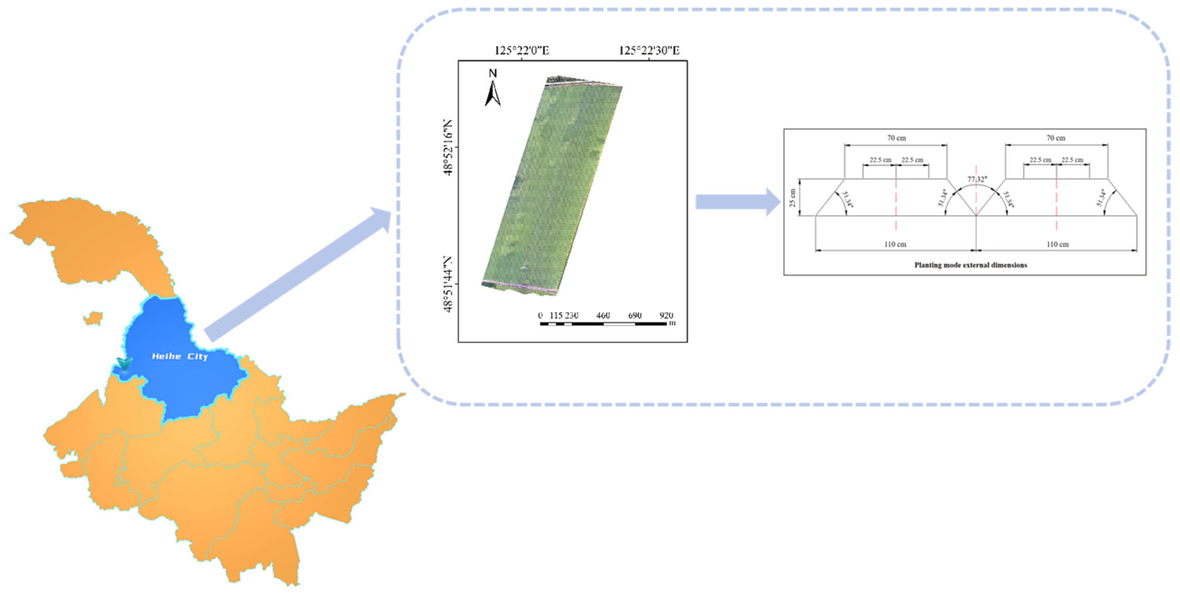
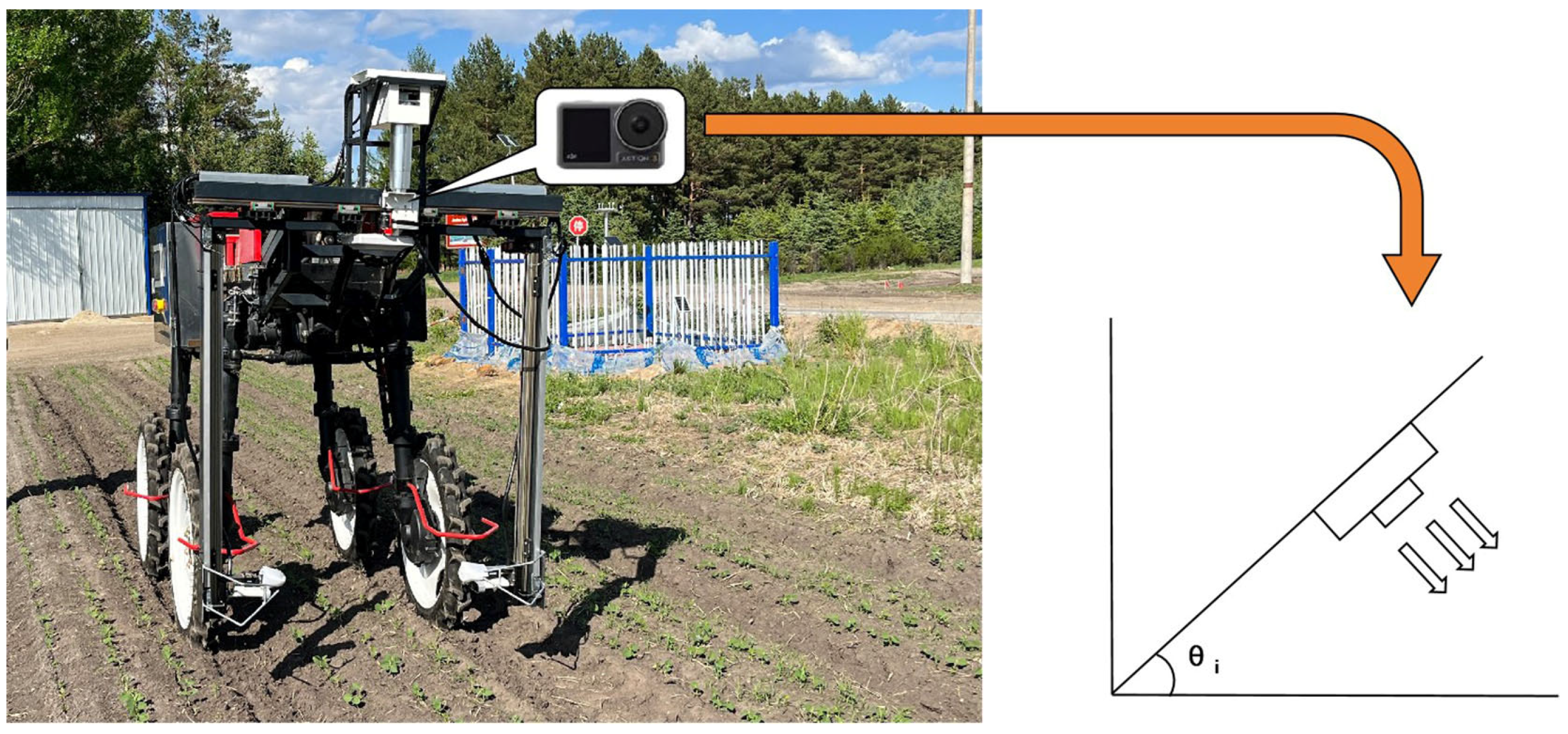
2.1. Image Acquisition

This research focused on soybean at the seedling stage, and the experimental site was situated in Jianshan Farm Science and Technology Park, Heihe City, Heilongjiang Province, China (48°52′17.16″ N, 125°25′9.40″ E), where data were collected during the experiment. Soybeans are planted in a three-row pattern on ridges, as illustrated in Figure 1. The ridge base width is 110 cm, the ridge top width is 70 cm, the height is 25 cm, the angle between two ridges is 77.32°, and the slope angle of the ridge top is 51.34°. Three rows of soybeans are planted by offsetting the centre line to the left and right by 22.5 cm on each ridge top.

Image data acquisition of soybean at the seedling stage was carried out, and the image acquisition equipment used a DJI Omso Action3 camera(SZ DJI Technology Co., Ltd., Shenzhen, China) with a field of view of 155°, focal length up to 50 cm, image resolution up to 4000 pixels × 3000 pixels, and acquisition speed of 60 f/s. RGB images can be captured; the image storage format was JPEG/RAW. The DJI Omso Action3 camera’s high resolution and colour contrast can make the difference between soybean seedlings and the field background more obvious, and it also has a stabilisation function to prevent jitter during image acquisition from affecting the quality of image acquisition and image processing results.

With the image sensor placed at the centre line of the soybean information collection vehicle. Most of the smart agricultural equipment are applied in the field environment; so in this study, the shooting angle and light intensity of acquiring RGB images are selected as variables for image acquisition based on the actual situation in the field and the viewing distance of the smart agricultural equipment. The multi-level visible light image acquisition of soybean in the seedling stage was conducted at multiple shooting angles (angles with the ground) and various light intensities. The shooting angles were set to θ with the ground at three levels: 0°, 45°, and 90°. The acquisition of soybean seedling stage images was conducted under both sunny and cloudy weather conditions, with the schematic diagrams illustrating the placement position and shooting angle of the image sensor shown in Figure 2.

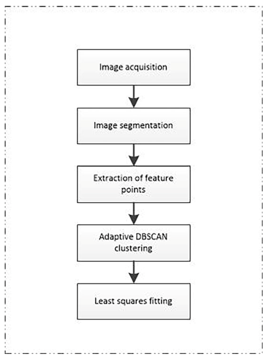
2.2. Algorithm for Soybean Seedling Navigation Line Extraction

Algorithm writing is performed using PyCharm, and the subsequent research is conducted with the OpenCV computer vision library. The algorithm can be divided into five parts, ranging from image segmentation to navigation line extraction. Image segmentation is performed on the RGB image captured by the image sensor, and the green component of the soybean seedling belt is extracted to obtain a grayscale map. Feature point extraction is performed using the binarised image obtained from image segmentation. The algorithm is implemented based on the feature point extraction method proposed in this paper. The feature points are obtained and clustered using the adaptive DBSCAN clustering algorithm. Then, the centreline of the crop rows is fitted, and the navigation lines are extracted using the least squares method for the clustered set of feature points. The flowchart is shown in Figure 3.

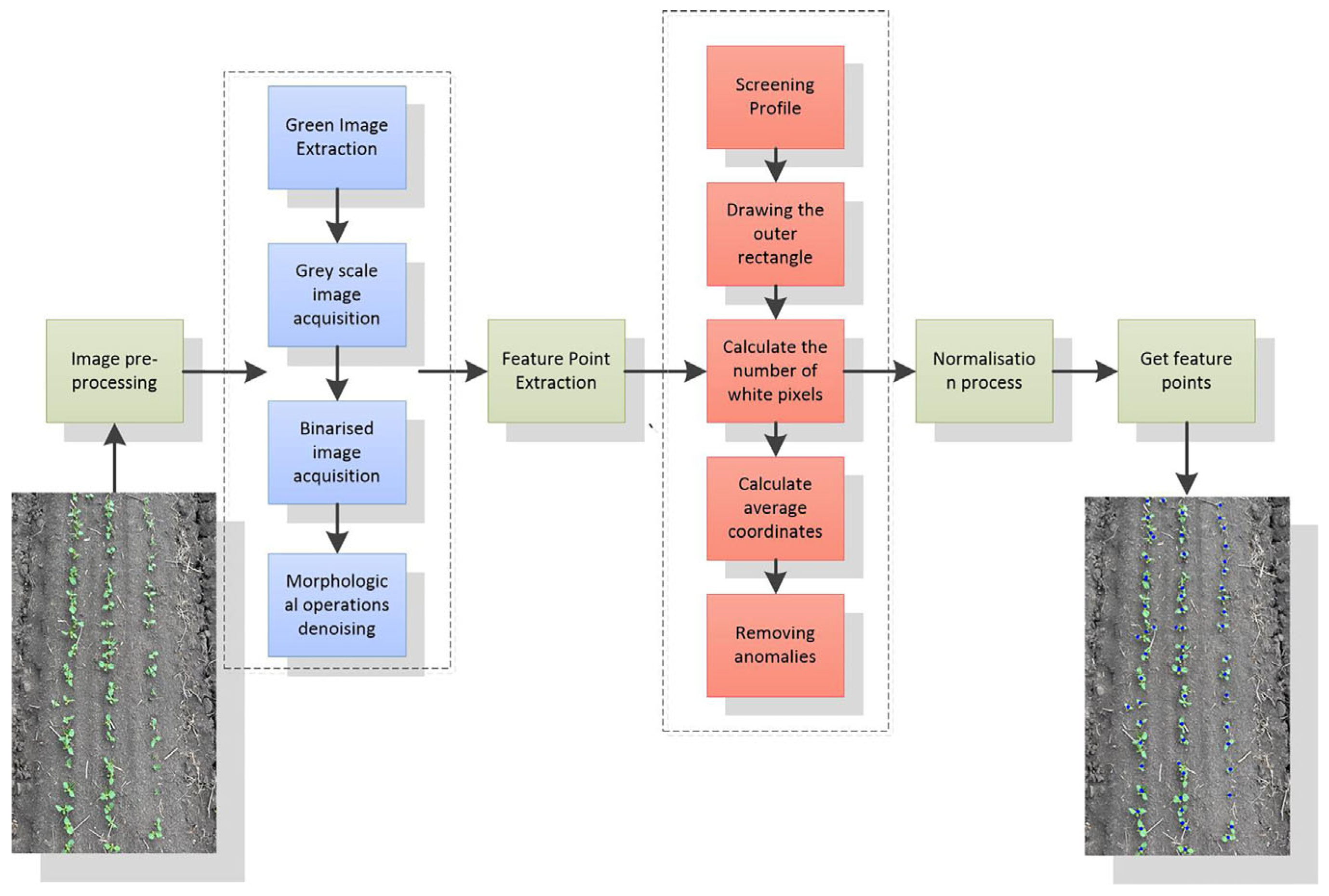
2.3. Image Segmentation

2.3.1. Image Greyscaling and Binarisation

The purpose of greyscaling the image is to distinguish the soybean seedling band from the complex field background. The field environment is characterised by various elements such as straw, weeds, soil, and other backgrounds, which can introduce interference in soybean seedling images and impact the accuracy of crop row centreline fitting. The collected RGB images of soybean seedlings exhibit green as the predominant colour component in the crop rows, which is notably distinct from the background colour of the field [18,19,20,21]. The HSV colour model was selected to effectively separate the green images of the soybean seedling crop rows from the background, enabling efficient extraction of their green features [22]. That is, based on hue, saturation, and brightness, the minimum and maximum ranges of HSV values are set. Equation (1) is as follows:

minGreen = [H_min,S_min,V_min]
maxGreen = [H_max,S_max,V_max]

(1)

The minimum value of the H channel in the green area is referred to as H_min, while the maximum value of the H channel is denoted as H_max. Similarly, S_min represents the minimum value of the S channel within the green area, whereas S_max represents its maximum value. V_min indicates the minimum value of the V channel in relation to the green area, while V_max denotes its maximum value. The obtained results are derived through processing. Figure 4 illustrates the outcome of extracting a green image from a soybean seedling band using the HSV colour model.

The pixels belonging to the green component are assigned a value of 255 according to Equation (2), while the remaining pixels are set to 0, resulting in the extraction of the green component.

Gi = 2G − R − B

(2)

The pixel values of the three channels are weighted to obtain the final grayscale level and then converted into a grayscale image. This method of converting to grayscale completely separates the grayscale image of soybean seedlings from the background, which is beneficial for subsequent processing steps. The greyscale image is thresholded using the OTSU method [23,24] to obtain a binarised image. This technique automatically determines an optimal threshold for segmenting the greyscale image into background and foreground components. By converting the greyscale image, the background is rendered black, facilitating clear differentiation from the target image and enabling effective binarization.

$$\mathrm{B}(\mathrm{i},\mathrm{j})=\left\{\begin{array}{c}0,\mathrm{p}(\mathrm{i},\mathrm{j})<\mathrm{thresh}\\ 255,\mathrm{p}(\mathrm{i},\mathrm{j})\ge \mathrm{thresh}\end{array}\right.$$

(3)

The pixel value of point (i, j) in the image is represented as p(i, j) in Equation (3), where i = 0, 1, 2, … and j = 0, 1, 2, … Here, i represents the grayscale value of point (i, j) in the image. B(i, j) refers to the corresponding grayscale value of point (i, j) in the binarised image. The optimal threshold of a grayscale image can effectively separate the crop rows from the background by segmenting all pixels into two parts: crop rows and background. In the binarised image, the region with B(i, j) = 0 represents the background, while the region with B(i, j) = 255 corresponds to plants or noise points obtained through the aforementioned method.

2.3.2. Morphological Operations

Noise in the image is processed using morphological closure operations on binarised images, where the dilation operation is performed on the binarised image, followed by the erosion operation to fill holes, smooth object edges, and connect neighbouring object regions. The formula can be expressed as Equation (4):

$$\left(A·B\right)=\left(A\oplus b\right)\ominus b$$

(4)

In Equation (4), A denotes the original image, B denotes the structural elements, $\oplus$ and $\ominus$ represent both the expansion operation and the erosion operation. Additionally, a 3 × 3 matrix filled with all ones is set as the convolution kernel for morphological processing. The holes in the mask are filled through morphological closure operations to enhance the continuity and completeness of the entire object region. This process also smooths the edges of the binarised image, eliminates fine noise, and improves the accuracy of crop row centreline recognition.

2.4. Feature Point Extraction

The extraction of feature points is an essential prerequisite for detecting the centreline of crop rows. In this study, soybean is chosen as the research object, and a monopoly planting method with three rows on the ridge is employed, allowing us to consider the positional relationship between each crop row as a linear parallel relationship. The experimental field is located in Jianshan Farm, Jiusan Bureau, Heihe City, Heilongjiang Province. The row-spacing and plant-spacing of soybean seedlings are relatively fixed. Soybean seedling plants have a small size and a nearly round plant morphology. A feature point extraction method is proposed by calculating the average coordinates of the pixel points of the plants in the soybean seedling belt. The average coordinates of white pixel points of soybean plants are calculated under a specific threshold to ensure that the extracted feature points are precisely located on the plants, thereby enhancing the accuracy of recognising the centre line of the crop row.

The specific feature point extraction steps are as follows:

• A suitable threshold value, Thresh, is set according to the size of the binarised image of soybean seedlings. The seedlings in the binarised image that meet this specific threshold value are calculated. The contours of each soybean seedling in the binarised image are traversed and compared with the specific threshold value. Contours smaller than the set threshold value are ignored.
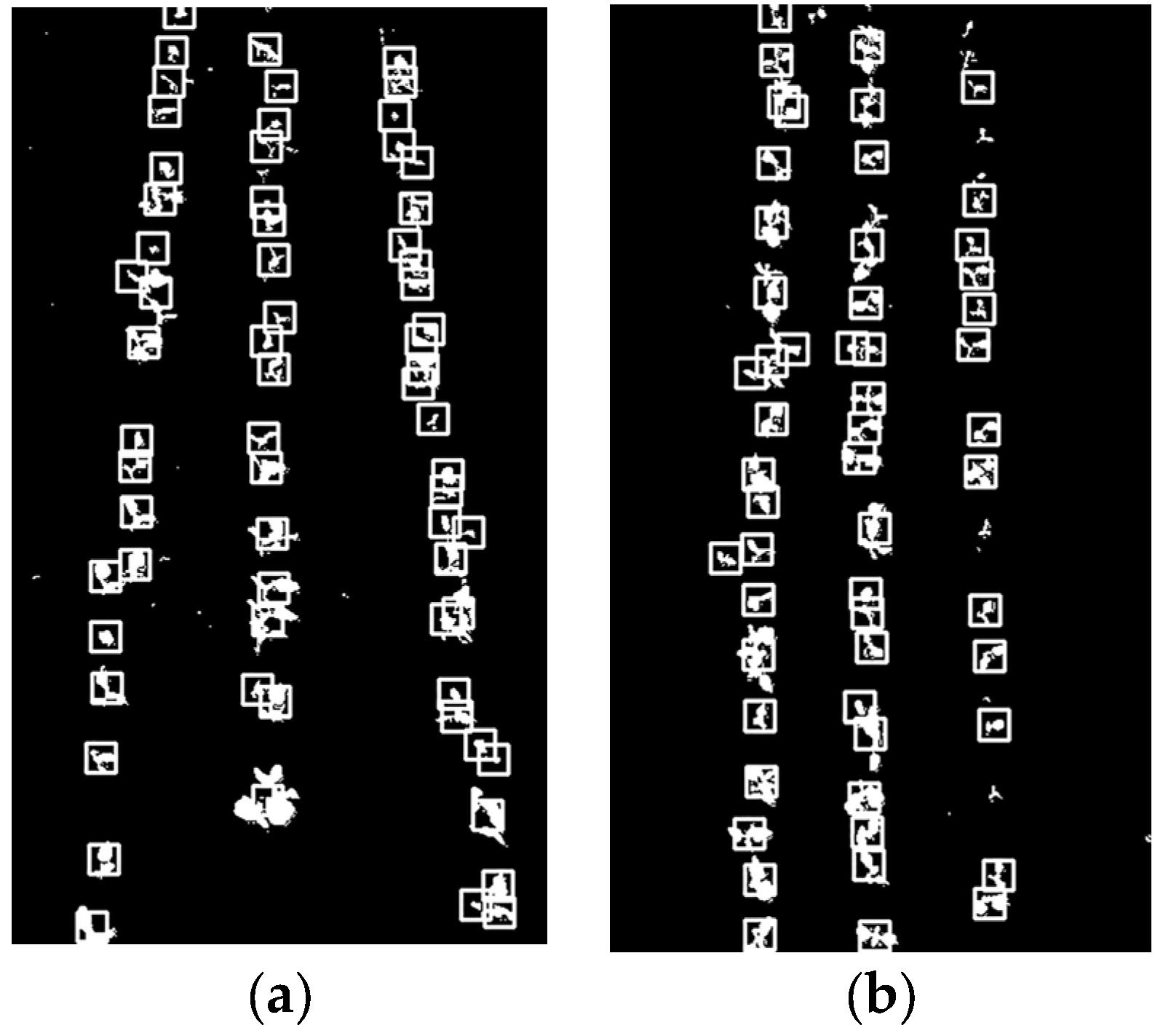
• Iterate over the contour that meets the set threshold, use the OpenCV function to calculate the coordinates and dimensions of the rectangular box for this contour, and calculate the area of the binarised image contour that satisfies these conditions. The minimum value of the binarised image contour area is denoted as S_t, and the eligible contour area is denoted as S. The width and height of the bounding rectangle, denoted as w and h, respectively, can be calculated for an image contour with an area of S. The top-left corner coordinates (x, y) represent the offset. Figure 5 shows the result of drawing a bounding rectangle on a binary image of soybean seedlings after traversing the contours.
• Calculate the number of white pixels, n, within the bounding rectangle. Meanwhile, soybean seedlings exhibit diverse plant morphologies during their growth process. To avoid issues such as feature point displacement caused by small plants, a specific threshold, Threshi, is set again. If the number of white pixels within the bounding rectangle exceeds this threshold, further processing will be applied to contours that meet this condition.
• The non-zero pixel points within the outer rectangle that satisfy the given conditions should be identified, and their average coordinates should be calculated. The average value of these coordinates (a, b) should then be computed and added to the offsets x and y of the rectangular box as stated in Equation (5).

  $$\begin{gathered} \mathrm{a}={\displaystyle \frac{1}{\mathrm{N}}}{\sum }_{\mathrm{i}=1}^{\mathrm{N}}(\mathrm{n}\mathrm{o}\mathrm{n}\_\mathrm{z}\mathrm{e}\mathrm{r}\mathrm{o}\_\mathrm{p}\mathrm{o}\mathrm{i}\mathrm{n}\mathrm{t}\mathrm{s}[\mathrm{i},0])+\mathrm{x} \\ \mathrm{b}={\displaystyle \frac{1}{\mathrm{N}}}{\sum }_{\mathrm{i}=1}^{\mathrm{N}}(\mathrm{n}\mathrm{o}\mathrm{n}\_\mathrm{z}\mathrm{e}\mathrm{r}\mathrm{o}\_\mathrm{p}\mathrm{o}\mathrm{i}\mathrm{n}\mathrm{t}\mathrm{s}[\mathrm{i},1])+\mathrm{y} \end{gathered}$$

  (5)

  where N is the total number of non-zero pixel points; $\mathrm{n}\mathrm{o}\mathrm{n}\_\mathrm{z}\mathrm{e}\mathrm{r}\mathrm{o}\_\mathrm{p}\mathrm{o}\mathrm{i}\mathrm{n}\mathrm{t}\mathrm{s}[\mathrm{i},0]$ and $\mathrm{n}\mathrm{o}\mathrm{n}\_\mathrm{z}\mathrm{e}\mathrm{r}\mathrm{o}\_\mathrm{p}\mathrm{o}\mathrm{i}\mathrm{n}\mathrm{t}\mathrm{s}[\mathrm{i},1]$ are the x and y coordinates of the ith non-zero point, respectively, to obtain the feature point coordinates (a,b).
• The process of extracting the feature points will be affected by problems such as weeds, more seedlings, poor neatness, etc., and will be judged as an outlier based on the mean and standard deviation of the distance to the feature points, assuming that the distance is a P = {p₁, p₂, …, p_n} set of points, where each point pi is a d-dimensional vector. Calculate the distance matrix D, where D_ij denotes the distance between point p_i and point p_j:

  $${\mathrm{D}}_{\mathrm{i}\mathrm{j}}=\mathrm{d}\mathrm{i}\mathrm{s}\mathrm{t}({\mathrm{p}}_{\mathrm{i}},{\mathrm{p}}_{\mathrm{j}})$$

  (6)

Then, the mean value of the distance to the ith point can be expressed as $\mathsf{\mu }$_i:

$${\mathsf{\mu }}_{\mathrm{i}}={\displaystyle \frac{1}{\mathrm{n}-1}}{\sum }_{\mathrm{j}\ne \mathrm{i}}{\mathrm{D}}_{\mathrm{i}\mathrm{j}}$$

(7)

The standard deviation of the distance to the ith point can be expressed as $\mathsf{\sigma }$_i:

$${\mathsf{\sigma }}_{\mathrm{i}}=\sqrt{{{\displaystyle \frac{1}{\mathrm{n}-1}}{\sum }_{\mathrm{j}\ne \mathrm{i}}\left({\mathrm{D}}_{\mathrm{i}\mathrm{j}}-{\mathsf{\mu }}_{\mathrm{i}}\right)}^2}$$

(8)

The feature points whose distance standard deviations exceed three times the distance mean are considered outliers and removed to obtain the feature points. The selected feature points are then normalised, allowing them to be better adapted to the soybean seedling with the crop row extraction algorithm. This normalisation process ensures that different features are scaled uniformly, facilitating further analysis and processing. By calculating the mean and standard deviation of the feature point set in the column direction, subtracting the mean value from the feature point array to obtain the offset of each feature relative to the mean value, dividing the offset by the standard deviation to obtain the normalised value of each feature point, the normalised feature point array, i.e., the feature point set, is finally obtained. Figure 6 is the schematic diagram for the process of extracting the feature points of crop rows.

2.5. Navigation Line Extraction

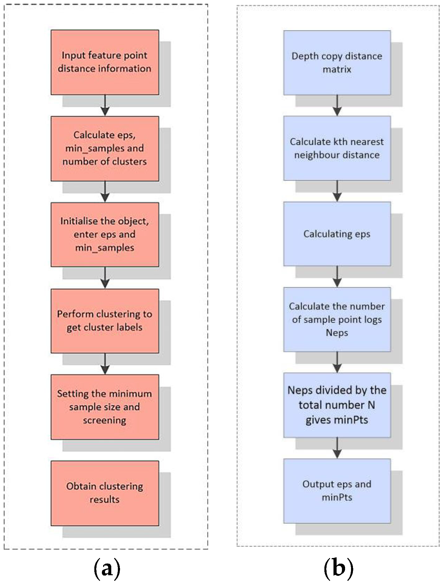
2.5.1. Feature Point Clustering

Crop row centreline detection for soybean seedling bands can be viewed as fitting a straight line to the soybean seedling feature points. In order to determine the exact location of the crop rows, it is necessary to determine the number of rows of soybean seedling bands that can be detected in the RGB image clustered according to the proximity between the extracted feature points. The occurrence of multiple seedlings during sowing leads to a situation where an excessive number of feature points representing a crop are present at the same or similar locations, thereby not only increasing the computational effort required for straight line fitting but also impacting the outcomes of such fitting.

According to the way of soybean cultivation, the extracted feature points can be roughly identified as three straight lines, whose clustering shapes are non-circular, and the density is relatively fixed; so this study uses DBSCAN clustering that can automatically cluster data points of arbitrary shapes [25,26,27]. The two key parameters of the DBSCAN clustering algorithm are the radius of neighbourhood and the minimum number of samples, which has the advantage of making the algorithm relatively convenient and reducing the subjectivity of parameter selection. However, for the unprocessed feature point set, the parameter setting is not accurate enough, and the parameters need to be set manually for different feature point recognition results, which cannot be applied in practical applications. If the parameters of the clustering algorithm can be calculated automatically through the calculation of the algorithm, efficiency will be greatly improved; so, in order to improve the adaptability of the clustering algorithm and the wide range of practical applications, the DNSCAN clustering algorithm is improved, which can adaptively identify the radius of the neighbourhood and the minimum number of samples, further improving the convenience and efficiency of the algorithm. The adaptive DBNSCAN clustering is achieved by calculating the Euclidean distance between two samples, returning the nth nearest set of distances, returning the average of the nth nearest set of distances, and returning the radius of the neighbourhood and the minimum number of samples for a given dataset. The flow of adaptive DBSCAN clustering is shown in Figure 7a.

Figure 7b shows the process of calculating parameters for adaptive DBSCAN clustering. In the process of adaptive DBSCAN clustering, initialization and setting of initial parameters are performed first. Based on these initial parameters, the neighbourhood density of each data point is calculated. When calculating the neighbourhood density of each data point, it is necessary to obtain two key parameters for DBSCAN clustering: neighbourhood radius (eps) and minimum number of samples (minPts). For each pair of sample points xi and yi in the dataset, their Euclidean distance d(x_i,y_i) is computed to form a distance matrix D with elements D_ij = d(x_i,y_i). The distances between each point and other points are sorted to obtain a distance sequence. The kth nearest distance is selected, and for each point, its average value is taken from the k-nearest distances D_k to determine the neighbourhood radius, as expressed in Equation (9):

$$\mathrm{e}\mathrm{p}\mathrm{s}={\displaystyle \frac{1}{\mathrm{N}}}{\sum }_{\mathrm{i}=1}^{\mathrm{N}}{\mathrm{D}}_{\mathrm{k}}\left(\mathrm{i}\right)$$

(9)

Among them, N is the total number of sample points, and D_k(i) is the kth nearest distance of the ith sample point. After obtaining the neighbourhood radius, we calculate the logarithm of the number of sample points with distances less than or equal to eps, denoted as Neps, and divide it by the total number of sample points N to obtain the minimum sample size. Finally, through clustering, feature points are divided into multiple clusters and labelled with different colours. Figure 8 shows the clustering results outputted by PyCharm. The identified crop row feature points in orange, blue, and green colours depict the spatial distribution of three rows of soybean seedlings within the planar coordinate system. The identified crop row feature points in orange, blue, and green colours depict the spatial distribution of three rows of soybean seedlings within the planar coordinate system. The identified crop row feature points in orange, blue, and green colours depict the spatial distribution of three rows of soybean seedlings within the planar coordinate system. These points are visualised as graphs in the PyCharm interface, facilitating easy observation of their distribution and clustering results.

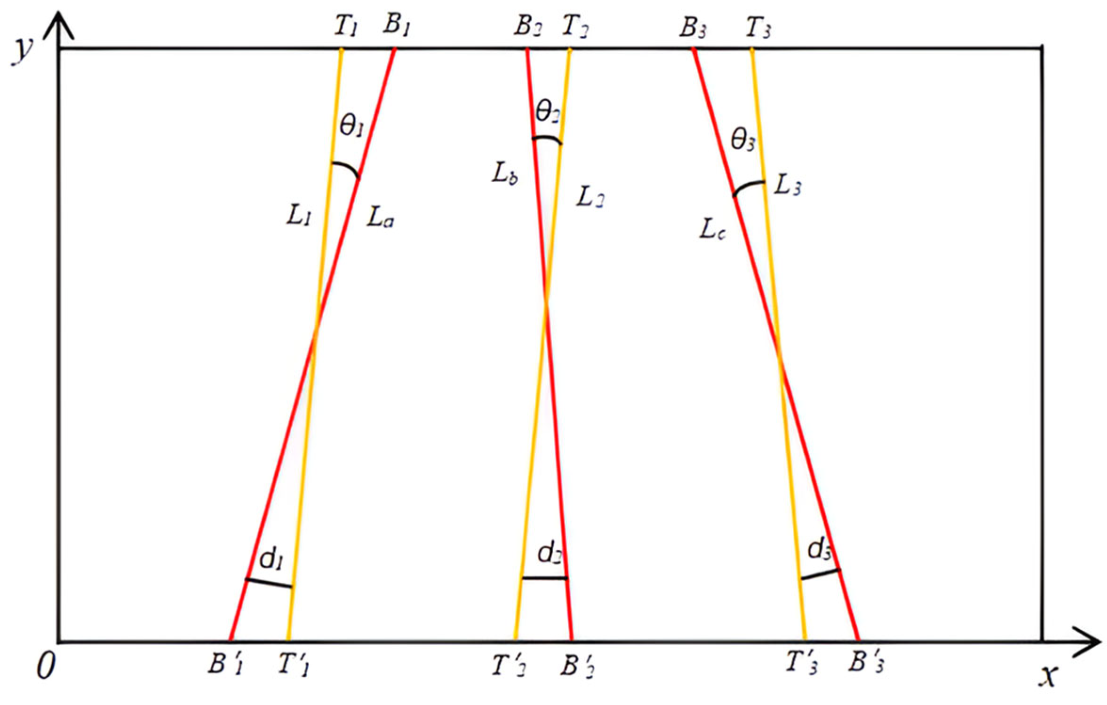
2.5.2. Crop Row Centreline Fitting and Navigation Line Extraction

Crop row identification is one of the core parts of the whole study, and the centre line of crop rows is obtained by linearly fitting the clustered feature points. The least squares method is selected for straight line fitting according to the feature point division, which can be a simple and direct linear calculation of data and obtain the fitting results, as well as has certain robustness [28].

The clustered feature points form a dataset containing a set of feature points (x_i, y_i), where i = 1, 2, …, N. The aim of the least squares method is to find a straight line such that the sum of the distances of all data points to this line is minimised. For the straight line y = mx + c, we can represent it in matrix form as in Equation (10):

$$\mathrm{Y}=\mathrm{A}\mathrm{X}$$

(10)

where Y is a column vector containing all yi coordinates, X is a column vector containing so xi coordinates, and A is a 2 × 2 matrix containing slope m and intercept c. For a given feature point, a system of linear equations Y = AX is constructed, and the coefficients m and c are solved for using the least squares formulation. The goal of the least squares method is to minimise the residual sum of squares S, as in Equation (11):

$$\mathrm{S}(\mathrm{m},\mathrm{c})={\sum }_{\mathrm{i}=1}^{\mathrm{N}}{\left({\mathrm{y}}_{\mathrm{i}}-{\mathrm{m}\mathrm{x}}_{\mathrm{i}}-\mathrm{c}\right)}^2$$

(11)

which is equivalent to solving the least squares solution of the system of linear equations Y = AX as in Equation (12):

$$\mathrm{A}={\left({\mathrm{X}}^{\mathrm{T}}\mathrm{Y}\right)}^{-1}{\mathrm{X}}^{\mathrm{T}}\mathrm{Y}$$

(12)

In the formula, XT represents the transpose of X, and ${\left({\mathrm{X}}^{\mathrm{T}}\mathrm{Y}\right)}^{-1}$ represents the inverse of matrix ${\mathrm{X}}^{\mathrm{T}}\mathrm{Y}$. By solving according to the given formula, in matrix A, the first element represents the slope m, and the second element represents the intercept c.

Using the obtained slope (m) and intercept (c), the centre line of the crop row was calculated and plotted. The maximum and minimum values of x in the point set were selected to determine the coordinates of both endpoints of the centre line, which were then extended on either side according to Equation (13):

$$\begin{gathered} x_1^{\prime }=x_{min}-line\_length, x_2^{\prime }=x_{max}+line\_length \\ {y}_1^{\prime }=m·x_1^{\prime }+c, y_2^{\prime }=m·x_2^{\prime }+c \end{gathered}$$

(13)

The endpoint coordinates were calculated by Equation (13), and a straight line was fitted to obtain the crop row centre line. Linear regression was performed based on the extracted feature points and crop row centre line to obtain the navigation line.

3. Results

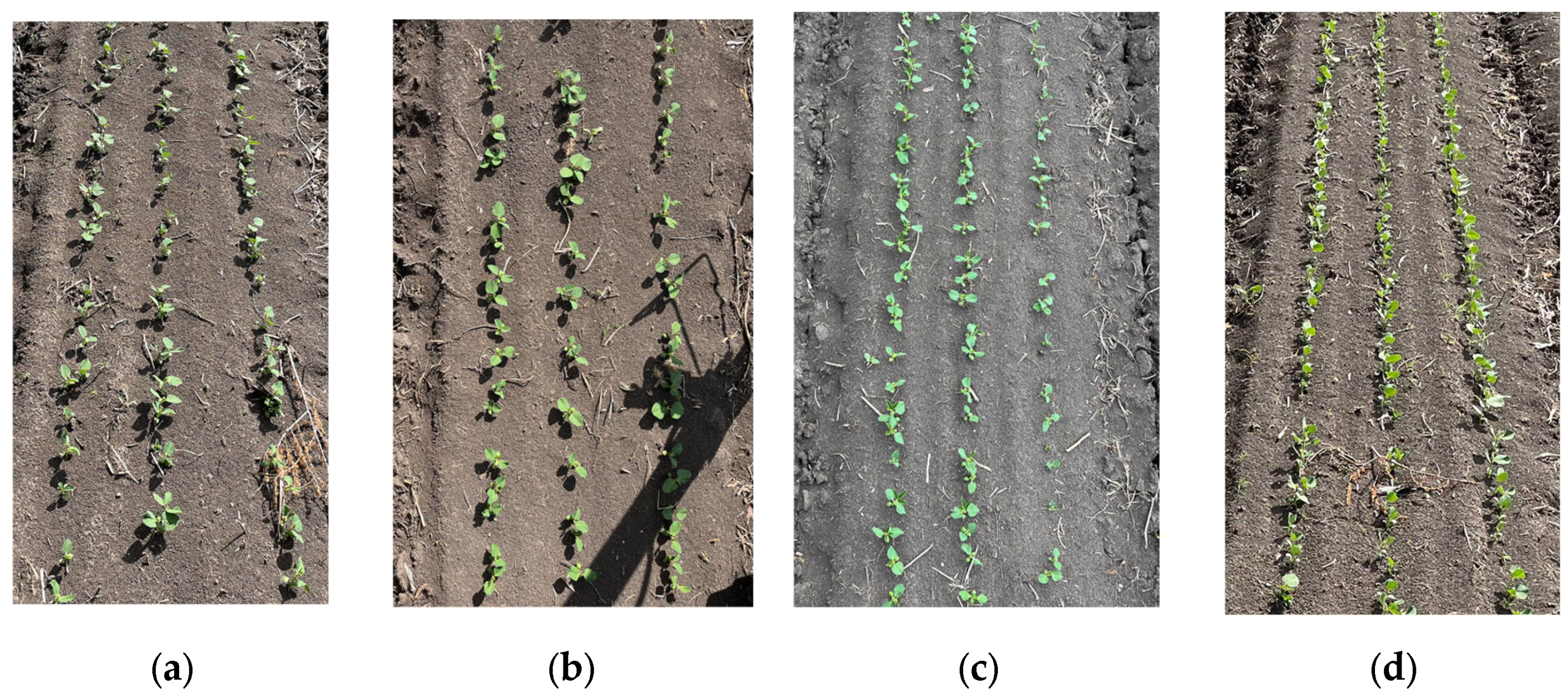
3.1. Acquisition of Visible Light Images of Soybean Seedling Strips

RGB images of soybean seedling strips at multiple levels were acquired by an image sensor, and four selected original images are shown in Figure 9 as a, b, c, and d, respectively; Figure 9a is the original image taken at an angle of 45° on a sunny day; Figure 9b is the original image taken at an angle of 0° on a sunny day; Figure 9c is the original image taken at an angle of 0° with the presence of straw under cloudy weather; and Figure 9d is the original image taken at an angle of 90° with the presence of straw; and Figure 9d is the original image taken at an angle of 90° with the presence of straw on a sunny day.

The RGB images captured are of high quality overall and meet the image segmentation requirements. The quality of the RGB images captured under sunny and cloudy weather varies. From the results of the image acquisition, the shooting angle of the image sensor did not have an impact on the quality of the acquired images and the subsequent recognition. In the field environment, the light will shine directly on the soybean seedlings, and when the light intensity is high, it will affect the image acquisition of the green soybean seedlings, resulting in the green image edges of the soybean seedlings being missing in the process of image segmentation.

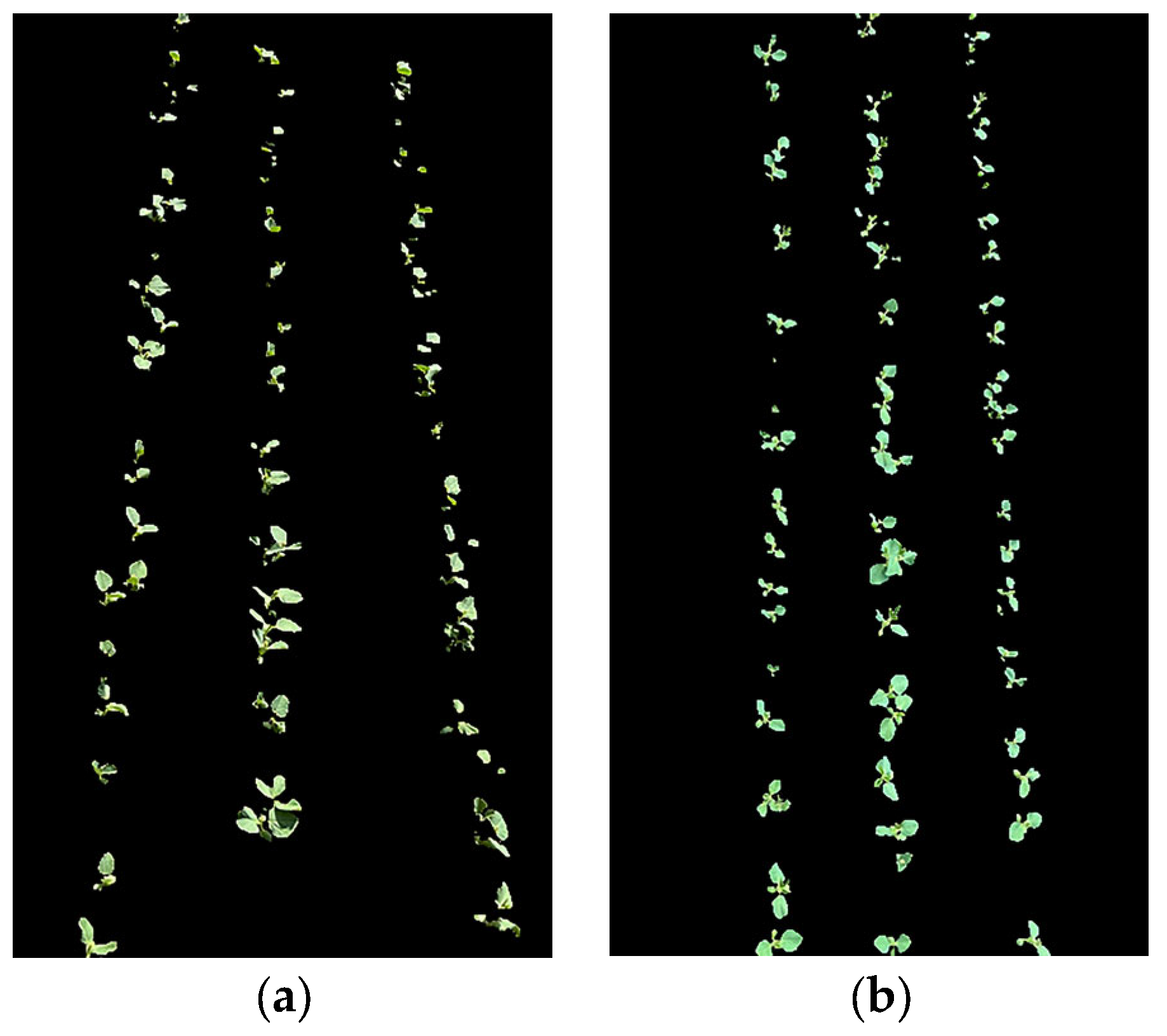
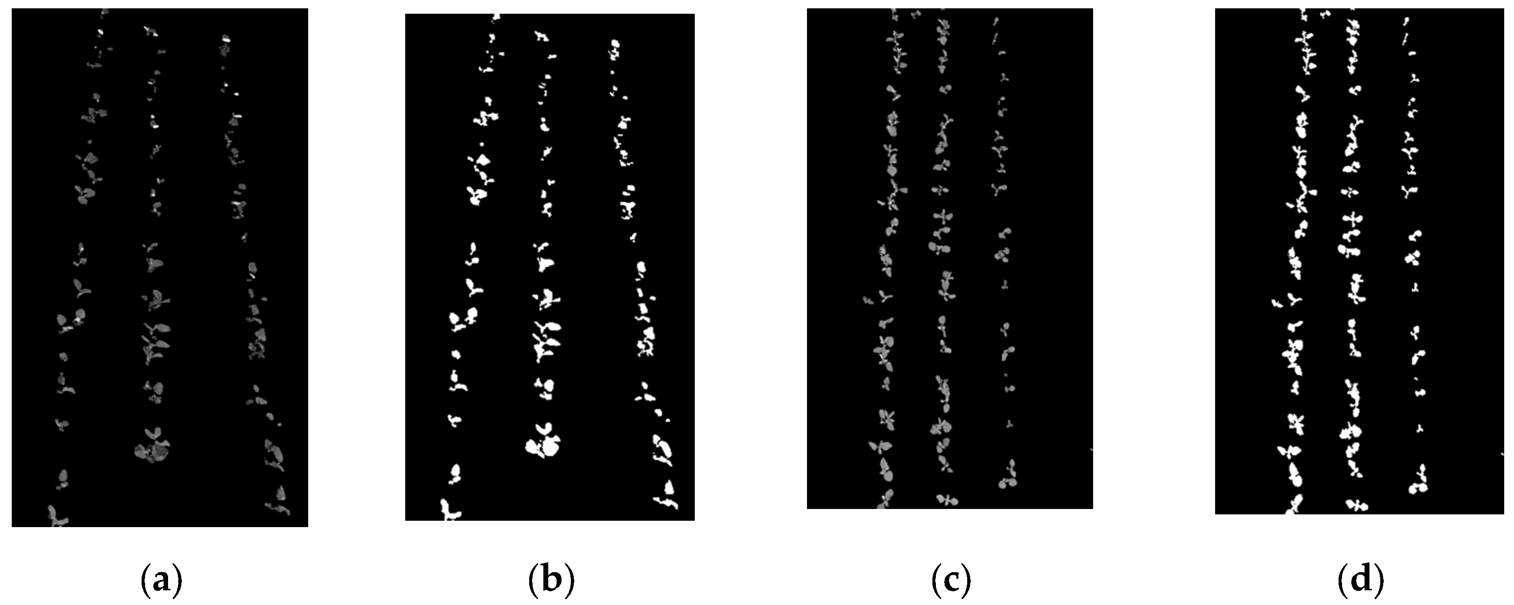
3.2. Image Pre-Processing

The original images in Figure 9a,c underwent image pre-processing. In a strong light environment, the original image Figure 9a was affected by lighting variations that result in shadows. Figure 10a illustrates the greyscale image obtained by extracting the green component from the original image under such conditions, enabling identification of the location of the soybean seedling belt. Figure 10b displays the binarised image achieved through OTSU method processing of the original image in Figure 9a. From the binarised image extraction results, it can be seen that the crop row contours extracted by the image segmentation method based on extracting the green image of the soybean seedling band are complete. Combining the processing effect of the original image c in low light (cloudy weather) and analysing it to obtain the grey scale image and binarised image processing results, in Figure 10c,d, it can be seen that the image segmentation method used in this study can be adapted to both sunny and cloudy light conditions.

In the image pre-processing process, due to the possible uneven distribution of artificially sown soybean seedlings, there will be a situation in which multiple soybean seedlings are connected together, binarised as in the connected region of Figure 10d, while the outer connecting rectangle is unable to box in the whole region due to the pre-set area threshold, resulting in the loss of feature points, which can be solved by adjusting the threshold value. At the same time, the emergence of the lack of seedlings and broken rows will also affect the subsequent research; the number of extractable feature points becomes less, and the clustered feature points have an impact on the accuracy of straight-line fitting, which may result in offset and recognition failure.

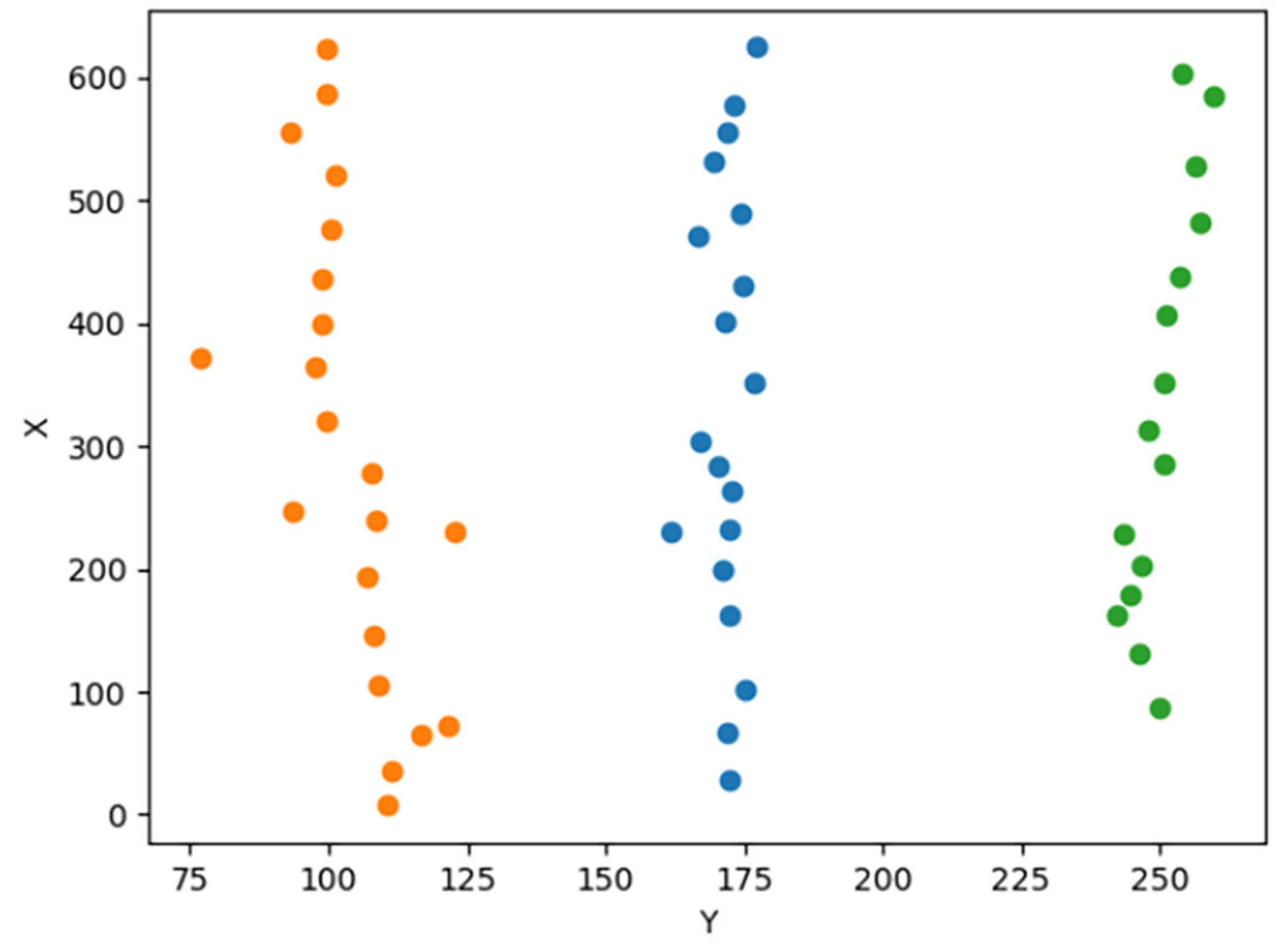
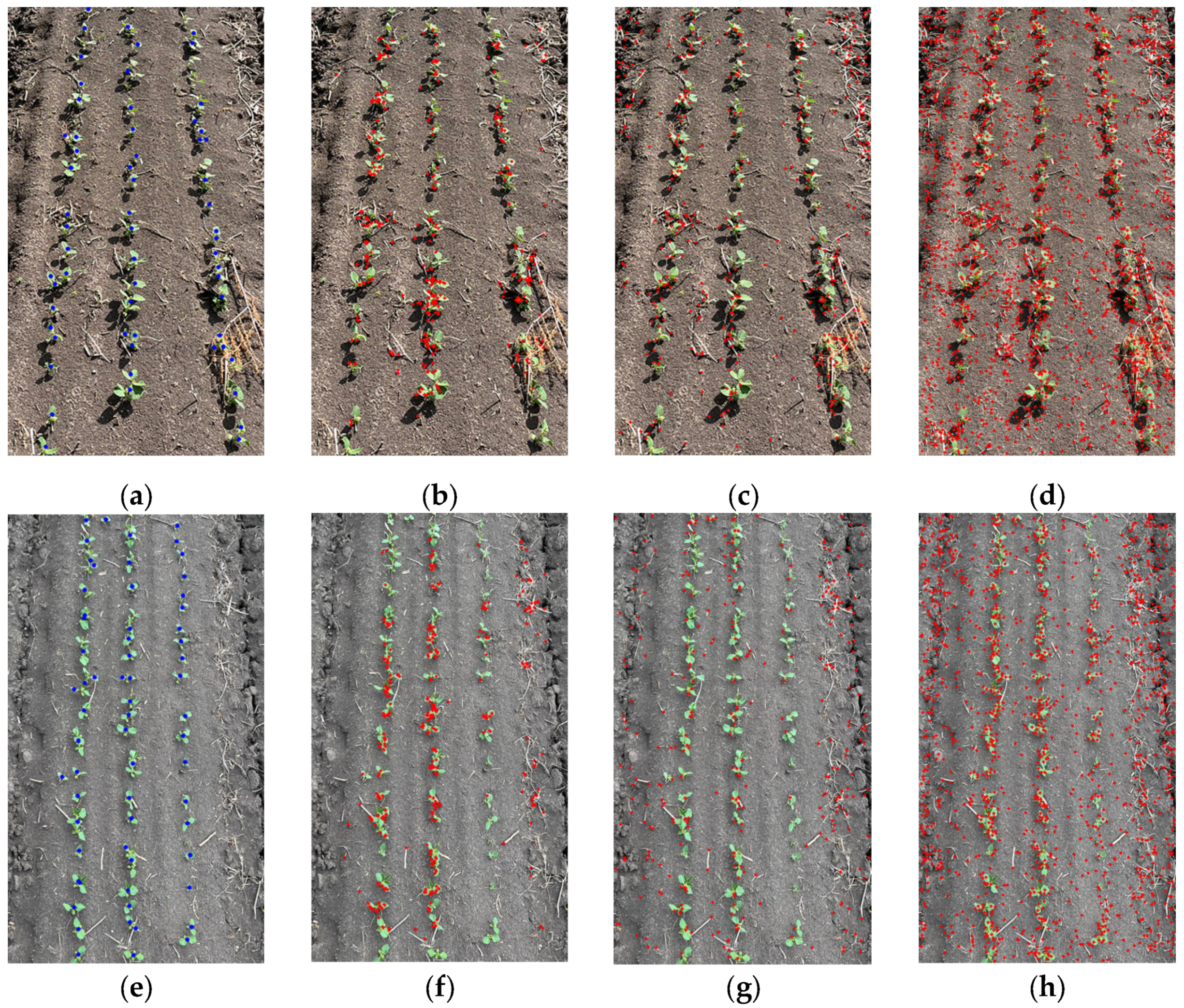
3.3. Feature Point Extraction and Clustering

This study proposes to extract feature points by calculating the average coordinates of the pixel points in the binarised image of a soybean seedling plant and calculating the average coordinates by drawing an outer rectangle on each plant contour. In the process of feature point extraction, the threshold value of the binarised image is set to ensure that each outer rectangle is drawn on the plant contour, so that the extracted feature points all appear in the original image of the soybean seedling, and the accuracy of feature point extraction is improved. For feature point detection, the commonly used methods include Harris corner point, Fast corner point, Sift corner point, etc. Although the extraction of feature points is based on the grey scale image and binarised image of the image, different feature point detection methods are different. Three feature point extraction methods, Harris corner point, Fast corner point, and Sift corner point, are compared with the feature point extraction method proposed in this paper.

The original images in Figure 11a,c are taken as examples for comparison, and the results are shown in Figure 11. Harris corner points, Fast corner points, and Sift corner points were used to extract feature points for the image with the presence of straw in sunny weather, respectively, and a large number of shadows of soybean seedlings appeared in the image because of the strong light. Figure 11b–d show the extraction results of Harris corner point, Fast corner point, and Sift corner point, respectively, and there is a significant difference between the three before. All three methods showed detection errors, with Harris corner point detection being unevenly distributed and less effective. Fast corner point detection and Sift corner point detection both incorrectly identified straw in the field, with Sift corner point detection having the greatest error. Harris corner point, Fast corner point, and Sift corner point detection are performed on the images with the presence of straw under cloudy weather, the results of which are shown in Figure 11. In the case of weak illumination and reducing the influence of shadows, the extraction results of the three corner point detection methods still show uneven distribution and detection errors.

As shown in Figure 11a,e, the feature point extraction method proposed in this paper has no offset, uniform distribution, fewer anomalies, and is not affected by the surrounding environment in terms of extraction accuracy. At the same time, this paper proposes an adaptive DBSCAN clustering method to cluster the feature points, which automatically calculates the two important parameters of DBSCAN clustering, namely the neighbourhood radius and the minimum number of samples, according to the characteristics of the feature point set in the clustering process. This method avoids the need to set different parameters for different feature points in the process of using DBCSAN clustering and uses the characteristics of DBSCAN clustering itself to transform the feature points of each crop row into multiple clusters. The feature point clustering results are generated by OpenCV, and the different colours of the feature point clustering results on each crop row can be observed intuitively, which improves the efficiency compared with the traditional DBSCAN clustering. The improved adaptive DBSCAN clustering algorithm was used to cluster the soybean seedling belt images after extracting the feature points on the original images Figure 9a–d. It can be seen from Figure 12 that the closer the extracted feature points are to the top, the closer the distance between the crop rows is, and the shooting angle of the image sensor does not have any effect on the improved clustering method to divide the clusters, and it can be seen that the clustering of the images taken from multiple angles under sunny and cloudy weather is effective. For the case mentioned above, regarding the impact of missing seedlings and broken rows on the accuracy of crop row fitting, the problem was improved by weighting the parameters of the adaptive DBSCAN clustering to enhance the robustness of the clustering.

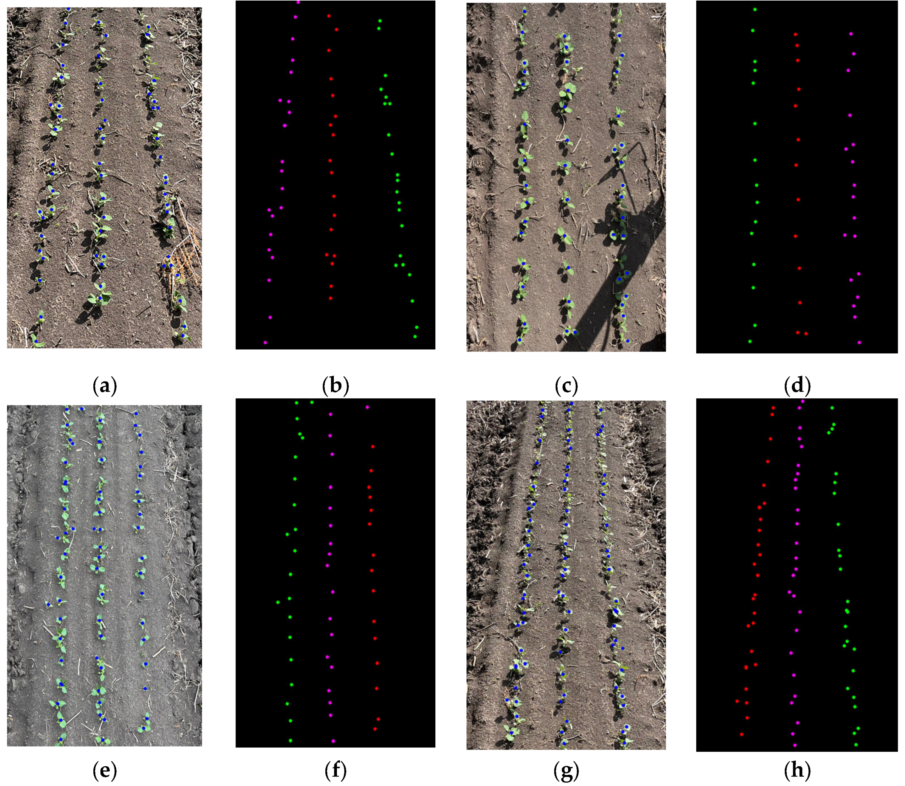
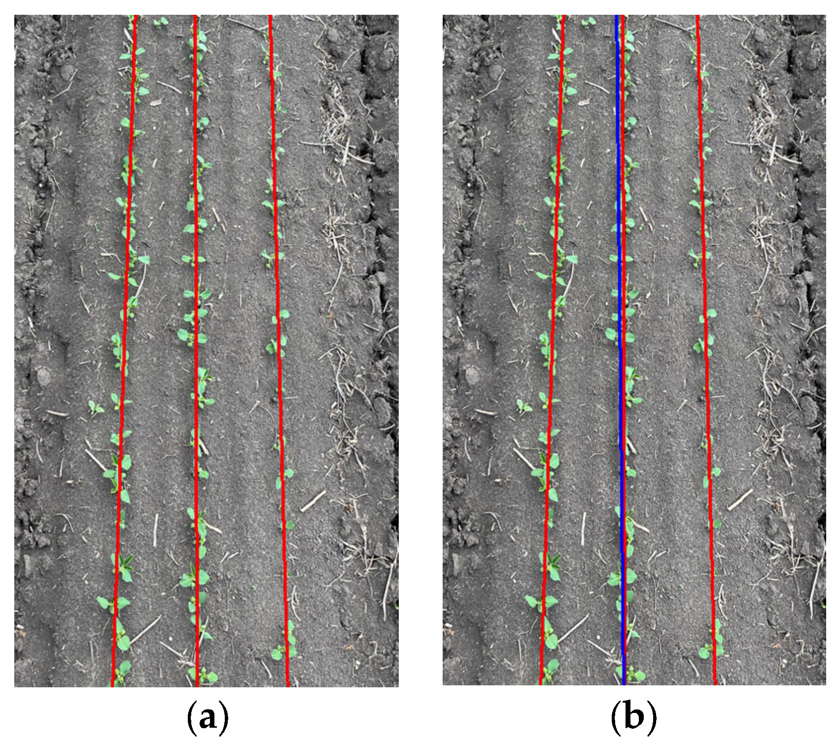
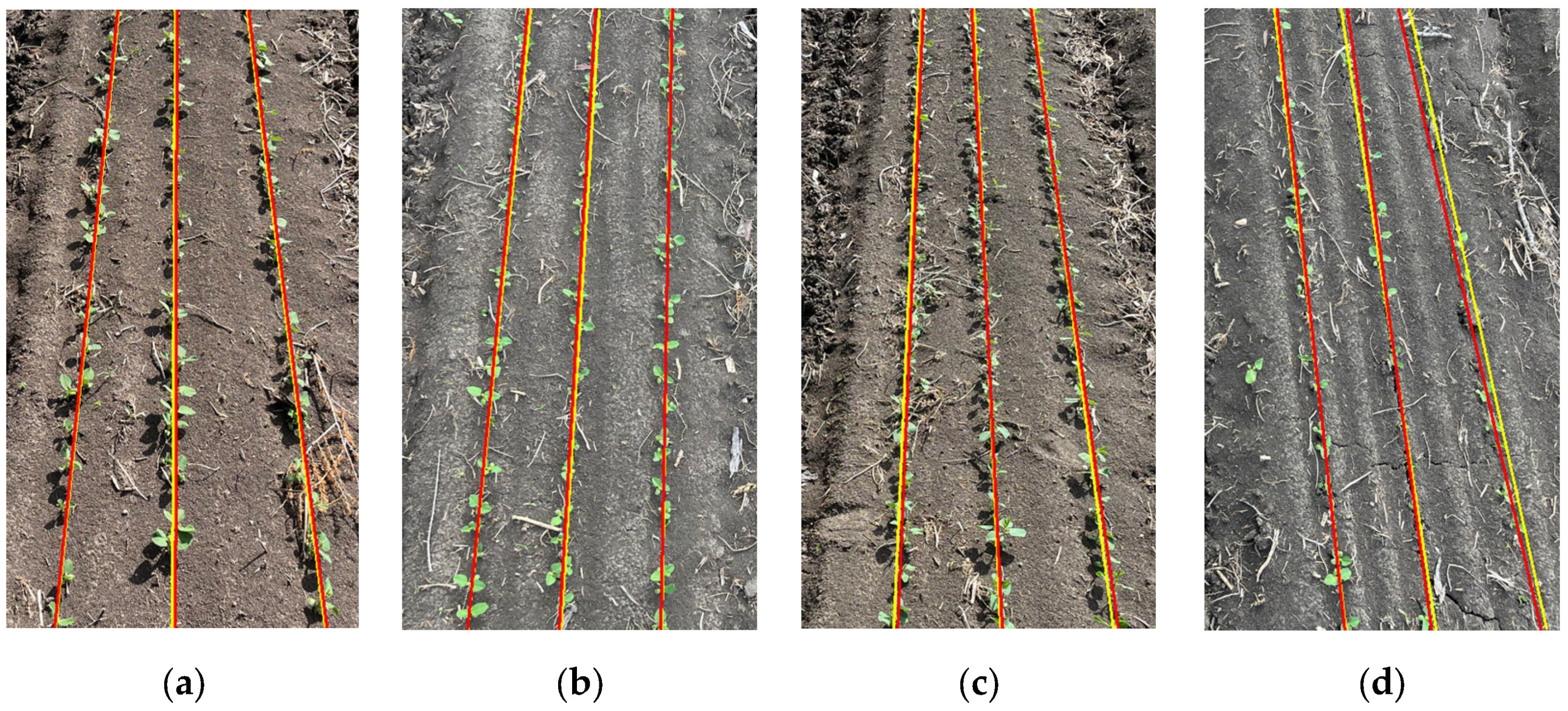
3.4. Experimental Results of the Verification of the Accuracy of the Fitting of the Navigation Line

In this study, the least squares method is used to fit the soybean seedling belt feature points to obtain the crop row centre line and navigation line, and the fitting results are shown in Figure 13, where the straight red line in Figure 13a is the fitting result of the crop row centre line, and the straight blue line in Figure 13b is the result of the navigation line extraction. From the results, it can be concluded that the method proposed in this paper can accurately extract the navigation lines between the rows of seedling soybeans for smart agricultural equipment.

Since the crop row centreline is estimated from the extracted feature points, the validation of the accuracy of the navigation line can be translated into the validation of the accuracy of fitting the crop row centreline. Twenty images were extracted from a multi-level sample to validate the navigation line extraction method in this study. Based on the findings of the validation of crop row centre line fitting in the literature [29], this paper uses a manually drawn straight line to compare with the fitted crop row centre line, and the manually drawn straight line is regarded as a standard line as a reference. In order to make the validation results more rigorous and accurate, the accuracy was verified by calculating the maximum distance error and angle difference between the fitted crop row centre line and the standard line.

As shown in Figure 14, it is assumed that L₁, L₂, and L₃ are standard lines, and L_a, L_b, and L_c are straight lines obtained by fitting through feature points. T₁, T₂, T₃, T′₁, T′₂, and T′₃ are the endpoint coordinates of the three standard lines, and B₁, B₂, B₃, B′₁, B′₂, and B′₃ are the endpoint coordinates of the three fitted straight lines. The angle of deviation θ between the fitted lines and the standard lines reflects the accuracy of the angular difference. θ₁ is the angle of deviation between L₁ and L_a. d₁ is the distance from L₁ to L_a; d₂ is the distance from L₂ to L_b; and d₃ is the distance from L₃ to L_c. Let the two endpoints of the hand-drawn line be (x₁, y₁) and (x₂, y₂), and the two endpoints of the fitted line be (x′₁, y′₁) and (x′₂, y′₂). Then, the slopes m1 and m₂ of the fitted and hand-drawn lines are calculated as in Equation (14):

$$\begin{gathered} {\mathrm{m}}_1=\mathrm{a}\mathrm{r}\mathrm{c}\mathrm{t}\mathrm{a}\mathrm{n}{\displaystyle \frac{{\mathrm{y}}_2-{\mathrm{y}}_1}{{\mathrm{x}}_2-{\mathrm{x}}_1}} \\ {\mathrm{m}}_2=\mathrm{a}\mathrm{r}\mathrm{c}\mathrm{t}\mathrm{a}\mathrm{n}{\displaystyle \frac{{\mathrm{y}\prime }_2-{\mathrm{y}\prime }_1}{{\mathrm{x}}_2-{\mathrm{x}\prime }_1}} \end{gathered}$$

(14)

Equation (15) for the angle θ₁ can be obtained from the slopes of the standard and fitted straight lines:

$${\theta }_1=arctan\left(\left|{\displaystyle \frac{m_2-m_1}{1+m_2{m}_1}}\right|\right)$$

(15)

θ₁ distinguishes between positive and negative values, which can indicate the relative position of L₁ and L_a, and thus the angular deviation value; absθ₁ is the absolute value of θ₁, which can indicate the degree of angular deviation. Meanwhile, the distance deviation distance d₁, d₂, d₃ from the standard line to the fitted straight line is calculated, and the distance deviation from the endpoints B₁, B₂, B₃ of the fitted straight line to the standard line L₁, L₂, L₃ is calculated by using the formula of the distance from a point to a straight line as in Equation (16):

$$\mathrm{d}={\displaystyle \frac{\left|\left({\mathrm{y}}_2-{\mathrm{y}}_1\right){\mathrm{x}}_3-\left({\mathrm{x}}_2-{\mathrm{x}}_1\right){\mathrm{y}}_3+{\mathrm{x}}_2{\mathrm{y}}_1-{\mathrm{y}}_2{\mathrm{x}}_1\right|}{\sqrt{{\left({\mathrm{y}}_2-{\mathrm{y}}_1\right)}^2+{\left({\mathrm{x}}_2-{\mathrm{x}}_1\right)}^2}}}$$

(16)

The meaning and calculation method of each group of straight-line parameters are the same. The distance deviation of each group of straight lines is averaged as the accuracy verification parameter for each image denoted by Avgd. The accuracy verification parameter for angular difference has the mean value of θ calculated for the three sets of straight lines and is denoted by Avgθ. The corresponding absAvgθ is calculated from the mean of absθ₁, absθ₂, and absθ₃. Avgθ and absAvgθ denote the angular difference value of the overall image and the degree of deviation in the overall image, respectively. Through the distance deviation analysis and angular difference analysis, the coincidence rate between the centre line of the fitted crop rows and the standard line was calculated to obtain the accuracy of the navigation line fitting A. Figure 15 shows the accuracy validation results of the images taken from the samples, where the straight red line is the result of the crop row fitting and the straight yellow line is the standard line. Figure 15a is the verification result of the image with 45° angle to the ground in sunny weather; Figure 15b is the verification result of the image with 45° inclination to the ground in cloudy weather; Figure 15c is the verification result of the image with 45° multi-straw in sunny weather; and Figure 15d is the verification result of the image with 45° inclination and lack of seedling in cloudy weather, and from the results, it can be seen that under the interference of the factors of sunny weather, cloudy weather, and multi-straw, the accuracy is still higher than the accuracy of the fit changes when there is a lack of seedlings in the image.

The results of accuracy validation parameters are obtained by calculating Avgθ, absAvgθ, Avgd, and A (see

Table 1. Mean Angle Difference vs. Absolute Mean Angle Difference.

Group	Avgθ					absAvgθ
a	−0.10	0.10	−0.03	0.14	0.30	0.17	0.10	0.04	0.20	0.30
b	−0.21	0.17	0.57	0.26	−0.02	0.53	0.31	0.57	0.32	0.20
c	−0.23	0.01	0.27	−0.42	−0.40	0.33	0.18	0.31	0.86	0.68
d	0.16	−0.06	0.10	−0.22	−0.18	0.16	0.12	0.42	0.38	0.22

and

Table 2. Average distance deviation and accuracy.

Group	Avgd					A
a	4.82	12.49	1.80	4.00	6.38	98.09%	98.40%	99.11%	97.96%	96.73%
b	10.64	6.62	12.38	7.28	5.02	94.74%	96.65%	93.65%	96.29%	97.50%
c	7.61	4.63	6.42	16.30	12.56	96.26%	97.69%	96.71%	91.97%	93.83%
d	3.34	2.88	8.92	7.94	5.50	98.29%	98.57%	95.51%	96.09%	97.30%

). The parameters show that the method fits a straight line with high accuracy, and the average accuracy of the four groups of samples is 96.77%, which meets the requirement of straight-line fitting, i.e., it meets the requirement of navigation line extraction.

From the analysis of the results of the four groups of samples at multiple levels in Table 1 and Table 2, the values of the four accuracy validation parameters are more stable, and the validation of the images at multiple levels under the conditions of sunny and cloudy (different light intensities) is good. As can be seen in Figure 15a–c, the red crop row centre line in the figure has a high overlap rate with the yellow standard line, which proves that the navigation line extraction approach proposed in this study has a good recognition effect. However, outliers appeared in the accuracy verification parameters of all four groups of samples, while the lack of seedlings appeared in the samples of the corresponding images. Soybean seeds in the field environment may be omitted and fail to germinate, resulting in a reduction in the feature point samples. In high light intensity conditions, due to the missing edges of the green image of soybean seedlings, the area of the binarised image is smaller than the actual area, resulting in a small number of feature points in the process of feature point extraction, which results in changes in the accuracy of navigation line extraction. After experiments and accuracy verification in the strong light conditions, navigation line extraction accuracy decreases, but most of them are maintained above 93%.

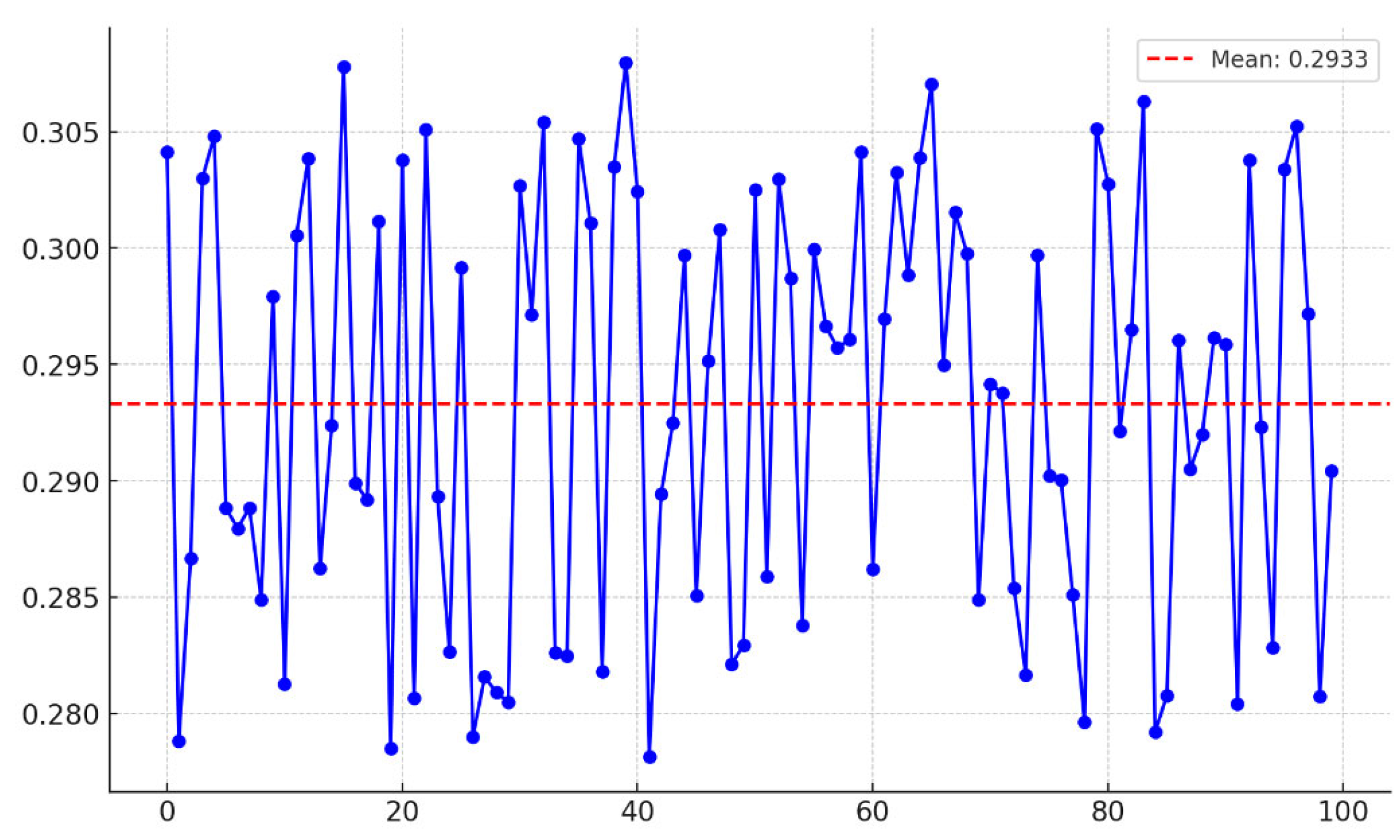
3.5. Timeliness Verification Test

The four sets of images underwent five rounds of processing using the aforementioned method, and the algorithm’s processing speed was assessed by incorporating a timing code in PyCharm during testing. The average execution time of the algorithm is 0.29 s (see Figure 16), demonstrating that its operational speed satisfies practical application requirements.

4. Discussion

4.1. Comparative Analysis of Related Studies

Many scholars have studied the crop row recognition methods from several aspects; García-Santillán et al. [30] and Zheng et al. [31] used image segmentation of crop rows using the RGB colour model to obtain binarised images; the image segmentation effect was better, but the binarised image had more noise. In this study, the HSV colour model and OTSU method were used for image segmentation to obtain the binarised image of soybean seedling completely with less noise. Zhao et al. [26] employed DBSCAN clustering to identify crop rows, yielding favourable recognition outcomes consistent with those of this study. Furthermore, enhancements to the DBSCAN clustering method in this research enable automatic parameter calculation and further improve the efficiency of cluster recognition. Ma et al. [32] proposed a robust crop root row detection algorithm based on linear clustering and supervised learning for crop root row detection in rice. The accuracy of crop root row detection was 96.79%, 90.82%, and 84.15% on the 6th, 20th, and 35th days of rice transplanting, respectively. Jiang et al. [33] proposed a simple and effective wheat row detection method including five steps of image segmentation, feature point extraction, candidate wheat row estimation, vanishing point detection, and real wheat row detection, and the detection rate reached 90%. The navigation line extraction method proposed in this study, which is based on the average coordinate of pixel points, achieves an accuracy rate of 96.77%, demonstrating superior recognition precision.

4.2. Algorithm Implementation Analysis

In this study, code was written using the OpenCV vision library in PyCharm for crop row recognition and navigation line extraction. The processor of the device used is a 2nd Gen Intel(R) Core(TM) i9-12900H(Lenovo, Beijing, China); the running memory is 32 GB, and the operating system used is Windows 11. The overall body of the code is on the lighter side, and the CPU occupancy at runtime is around 2%. In the pre-test, the initial code runs at a speed of 0.47 s.

In order to further improve the running efficiency of the code, the overall structure of the code was improved. By converting each functional body structure code into code blocks, the number of lines of code was reduced, the running speed was improved, and the average running speed was verified to be 0.29 s.

4.3. Challenges and Prospects

The proposed recognition method encompasses four key aspects: image segmentation, feature point extraction, feature point clustering, and crop row fitting. The feature point extraction method presented in this study is applicable to the entire soybean seedling stage for crop row recognition, detection, and navigation line extraction. Its effectiveness has been demonstrated in a field environment. The code runs at a speed of 0.29 s, which is adequate for real-time field applications. At the same time, because the algorithm runs more efficiently, it can accelerate the walking speed of intelligent agricultural equipment and improve the efficiency of recognition in practical applications.

However, there are still some problems that need to be improved. In the field environment, it is easy to be affected by high light intensity, which leads to a decline in the quality of image segmentation, resulting in a reduction in the accuracy of crop row recognition and navigation line extraction. In soybean sowing, there will be missed sowing, and in the growth process, a broken rows phenomenon appeared in the seedling, which will also lead to a decline in recognition accuracy. In this research method, we tried to improve image segmentation accuracy by extracting green images from the HSV colour model, and improve the efficiency of identifying missing seed rows by using an adaptive DBSCAN clustering algorithm. The accuracy has been improved, and the algorithm’s adaptability has been greatly improved, but it has not been fully solved. In the next step of research, how to solve the influence of light intensity and the occurrence of missing seed rows and broken rows will become the research focus.

This method will subsequently be applied to the acquisition equipment for practical field applications, with the aim of verifying that navigation lines can be accurately recognised despite the presence of various interference conditions in the field environment. From the experimental data and computational efficiency, the method is basically satisfied for large-scale operational identification in the field environment. Meanwhile, it also has great potential in terms of application scenarios, and this method can realise the extraction of most crop seedling images in farmland by extracting green images for image segmentation. The core of the proposed feature point extraction method that calculates the average coordinates of the pixel points is the calculation of pixel points, and is not specific to a single crop, which makes the navigation line extraction method of this applicable to a wide range of crops and environments for large-scale practical applications.

5. Conclusions

For field applications of automated driving of intelligent agricultural equipment between soybean ridges, we propose a multi-temporal navigation line extraction method that can be applied to soybean ridges in a field environment. By using the HSV model combined with the OTSU method to achieve image segmentation of soybean seedlings. The proposed method of calculating the average pixel coordinates to extract the feature points of soybean seedlings, which can accurately extract the feature points within the range of soybean seedlings and can cover the entire seedling process to the maximum extent. The improved adaptive DBSCAN clustering achieves automatic calculation of clustering parameters and clustering of feature points, and this clustering method improves the recognition efficiency and clustering quality. Crop rows and navigation lines were obtained by fitting using the least squares method. The method can satisfy the extraction of navigation lines in multiple time periods. By verifying the centre line of crop rows, the average distance deviation and the average angle deviation are 7.38 and 0.32, respectively, the accuracy of the fitted navigation lines is 96.77%, and the running speed is 0.29 s.

At the same time, the size of the specific threshold can be adjusted according to the change in plant size during the growth of soybean in the seedling stage, avoiding the impact of plant growth on feature point identification, so that the feature point extraction method proposed in this paper can cover the entire seedling stage to the maximum extent. Meanwhile, future research should focus on the effects of light intensity as well as seedling deficiency and row breakage on recognition accuracy in the field environment. This study provides a theoretical basis and support for the automatic driving of agricultural machinery between large field ridges and is also a further exploration of the field of automatic driving of agricultural machinery.

References

1. Jing, Y.; Li, Q.; Ye, W.; Liu, G. Development of a GNSS/INS-based automatic navigation land levelling system. Comput. Electron. Agric. 2023, 213, 108187. [Google Scholar] [CrossRef]
2. Romeo, J.; Pajares, G.; Montalvo, M.; Guerrero, J.M.; Guijarro, M.; Ribeiro, A. Crop row detection in maize fields inspired on the human visual perception. Sci. World J. 2012, 2012, 484390. [Google Scholar] [CrossRef]
3. Han, Y.; Wang, Y.; Sun, Q.; Zhao, Y. Crop Row Detection Based on Wavelet Transformation and Otsu Segmentation Algorithm. J. Electron. Inf. Technol. 2016, 38, 63–70. [Google Scholar]
4. Pang, Y.; Shi, Y.; Gao, S.; Jiang, F.; Veeranampalayam-Sivakumar, A.N.; Thompson, L.; Luck, J.; Liu, C. Improving crop row detection of early-season maize plants in UAV images using deep neural networks. Agric. Comput. Electron. 2022, 178, 105766. [Google Scholar] [CrossRef]
5. Shi, J.; Bai, Y.; Diao, Z.; Zhou, J.; Yao, X.; Zhang, B. Row detection BASED navigation and guidance for agricultural robots and autonomous vehicles in row-crop fields: Methods and applications. Agronomy 2023, 13, 1780. [Google Scholar] [CrossRef]
6. Diao, Z.; Guo, P.; Zhang, B.; Zhang, D.; Yan, J.; He, Z.; Zhao, S.; Zhao, C. Maize crop row recognition algorithm based on improved UNet network. Comput. Electron. Agric. 2023, 210, 107940. [Google Scholar] [CrossRef]
7. Liu, X.; Qi, J.; Zhang, W.; Bao, Z.; Wang, K.; Li, N. Recognition method of maize crop rows at the seedling stage based on MS-ERFNet model. Comput. Electron. Agric. 2023, 211, 107964. [Google Scholar] [CrossRef]
8. Zhou, J.; Geng, S.; Qiu, Q.; Shao, Y.; Zhang, M. A Deep-Learning Extraction Method for Orchard Visual Navigation Lines. Agriculture 2022, 12, 1650. [Google Scholar] [CrossRef]
9. Li, X.; Peng, X.; Fang, H.; Niu, M.; Kang, J.; Jian, S. Navigation path detection of plant protection robot based on RANSAC algorithm. Trans. Chin. Soc. Agric. Mach. 2020, 51, 40–46. [Google Scholar]
10. Zhou, Y.; Yang, Y.; Zhang, B.; Wen, X.; Yue, X.; Chen, L. Autonomous detection of crop rows based on adaptive multi-ROI in maize fields. Int. J. Agric. Biol. Eng. 2021, 14, 217–225. [Google Scholar] [CrossRef]
11. Zhou, X.; Zhang, X.; Zhao, R.; Chen, Y.; Liu, X. Navigation Line Extraction Method for Broad-Leaved Plants in the Multi-Period Environments of the High-Ridge Cultivation Mode. Agriculture 2023, 13, 1496. [Google Scholar] [CrossRef]
12. Li, X.; Zhao, W.; Zhao, L. Extraction algorithm of the center line of maize row in case of plants lacking. Trans. Chin. Soc. Agric. Eng. (Trans. CSAE) 2021, 37, 203–210. [Google Scholar]
13. Montalvo, M.; Pajares, G.; Guerrero, J.M.; Romeo, J.; Guijarro, M.; Ribeiro, A.; Ruz, J.J.; Cruz, J.M. Automatic detection of crop rows in maize fields with high weeds pressure. Expert Syst. Appl. 2012, 39, 11889–11897. [Google Scholar] [CrossRef]
14. Zhang, Q.; Chen, S.; Li, B. A visual navigation algorithm for paddy field weeding robot based on image understanding. Comput. Electron. Agric. 2017, 143, 66–78. [Google Scholar] [CrossRef]
15. Zhai, Z.; Zhu, Z.; Du, Y.; Zhang, S.; Mao, E. Binocular Visual Crop Row Recognition Based on Census Transformation. Trans. Chin. Soc. Agric. Eng. 2016, 32, 205–213. [Google Scholar]
16. Zhang, X.; Li, X.; Zhang, B.; Zhou, J.; Tian, G.; Xiong, Y.; Gu, B. Automated robust crop-row detection in maize fields based on position clustering algorithm and shortest path method. Comput. Electron. Agric. 2018, 154, 165–175. [Google Scholar] [CrossRef]
17. He, J.; Zang, Y.; Luo, X.; Zhao, R.; He, J.; Jiao, J. Visual detection of rice rows based on Bayesian decision theory and robust regression least squares method. Int. J. Agric. Biol. Eng. 2021, 14, 199–206. [Google Scholar] [CrossRef]
18. Garcia-Santillan, I.; Guerrero, J.M.; Montalvo, M.; Pajares, G. Curved and straight crop row detection by accumulation of green pixels from images in maize fields. Precis. Agric. 2018, 19, 18–41. [Google Scholar] [CrossRef]
19. Vidović, I.; Cupec, R.; Hocenski, Ž. Crop row detection by global energy minimization. Pattern Recognit. 2016, 55, 68–86. [Google Scholar] [CrossRef]
20. Burgos-Artizzu, X.P.; Ribeiro, A.; Guijarro, M.; Pajares, G. Real-time image processing for crop/weed discrimination in maize fields. Comput. Electron. Agric. 2011, 75, 337–346. [Google Scholar] [CrossRef]
21. Jiang, G.; Wang, Z.; Liu, H. Automatic detection of crop rows based on multi-ROIs. Expert Syst. Appl. 2015, 42, 2429–2441. [Google Scholar] [CrossRef]
22. Yang, Z.; Yang, Y.; Li, C.; Zhou, Y.; Zhang, X.; Yu, Y.; Liu, D. Tasseled crop rows detection based on micro-region of interest and logarithmic transformation. Front. Plant Sci. 2022, 13, 916474. [Google Scholar] [CrossRef] [PubMed]
23. Tenhunen, H.; Pahikkala, T.; Nevalainen, O.; Teuhola, J.; Mattila, H.; Tyystjärvi, E. Automatic detection of cereal rows by means of pattern recognition techniques. Comput. Electron. Agric. 2019, 162, 677–688. [Google Scholar] [CrossRef]
24. Otsu, N. A threshold selection method from gray-level histograms. Automatica 1975, 11, 23–27. [Google Scholar] [CrossRef]
25. Ruan, Z.; Chang, P.; Cui, S.; Luo, J.; Gao, R.; Su, Z. A precise crop row detection algorithm in complex farmland for unmanned agricultural machines. Biosyst. Eng. 2023, 232, 1–12. [Google Scholar] [CrossRef]
26. Zhao, R.; Yuan, X.; Yang, Z.; Zhang, L. Image-based crop row detection utilizing the Hough transform and DBSCAN clustering analysis. IET Image Process. 2024, 18, 1161–1177. [Google Scholar] [CrossRef]
27. Shi, J.; Bai, Y.; Zhou, J.; Zhang, B. Multi-Crop Navigation Line Extraction Based on Improved YOLO-v8 and Threshold-DBSCAN under Complex Agricultural Environments. Agriculture 2023, 14, 45. [Google Scholar] [CrossRef]
28. Bai, Y.; Zhang, B.; Xu, N.; Zhou, J.; Shi, J.; Diao, Z. Vision-based navigation and guidance for agricultural autonomous vehicles and robots: A review. Comput. Electron. Agric. 2023, 205, 107584. [Google Scholar] [CrossRef]
29. Yu, Y.; Bao, Y.; Wang, J.; Chu, H.; Zhao, N.; He, Y.; Liu, Y. Crop row segmentation and detection in paddy fields based on treble-classification otsu and double-dimensional clustering method. Remote Sens. 2021, 13, 901. [Google Scholar] [CrossRef]
30. García-Santillán, I.D.; Montalvo, M.; Guerrero, J.M.; Pajares, G. Automatic detection of curved and straight crop rows from images in maize fields. Biosyst. Eng. 2017, 156, 61–79. [Google Scholar] [CrossRef]
31. Zheng, L.Y.; Xu, J.X. Multi-crop-row detection based on strip analysis. In Proceedings of the 2014 International Conference on Machine Learning and Cybernetics, Lanzhou, China, 13–16 July 2014. [Google Scholar]
32. Ma, Z.; Tao, Z.; Du, X.; Yu, Y.; Wu, C. Automatic detection of crop root rows in paddy fields based on straight-line clustering algorithm and supervised learning method. Biosyst. Eng. 2021, 211, 63–76. [Google Scholar] [CrossRef]
33. Jiang, G.; Wang, X.; Wang, Z.; Liu, H. Wheat rows detection at the early growth stage based on Hough transform and vanishing point. Comput. Electron. Agric. 2016, 123, 211–223. [Google Scholar] [CrossRef]
Figure 1. Trial site and planting pattern.
Agronomy 14 01749 g001
Figure 2. Image sensor placement and shooting angle.
Agronomy 14 01749 g002
Figure 3. Soybean seedling navigation line extraction process.
Agronomy 14 01749 g003
Figure 4. HSV colour space green image extraction: (a) angle of 45° to the ground; (b) angle of 0° to the ground.
Agronomy 14 01749 g004
Figure 5. External rectangle drawing of binarised image: (a) angle of 45° to the ground; (b) angle of 0° to the ground.
Agronomy 14 01749 g005
Figure 6. Feature point extraction process.
Agronomy 14 01749 g006
Figure 7. Adaptive DBSCAN clustering process: (a) general flow chart; (b) eps and mimPts calculation process.
Agronomy 14 01749 g007
Figure 8. Adaptive DBSCAN clustering results.
Agronomy 14 01749 g008
Figure 9. Visible light images of soybeans collected under multiple conditions: (a) sunny day, 45° angle to the ground raw image; (b) sunny day, 0° angle to the ground raw image; (c) cloudy, 0° angle to the ground raw image, with straw; (d) sunny day, 90° angle to the ground, with straw raw image.
Agronomy 14 01749 g009
Figure 10. Image pre-processing results: (a) grayscale image under sunny weather; (b) binarised image under sunny weather; (c) grayscale image under cloudy weather; (d) binarised image under cloudy weather.
Agronomy 14 01749 g010
Figure 11. Comparison of the effect of feature point extraction: (a) sunny day, this paper’s extraction method; (b) sunny day, Harris corner detection; (c) sunny day, Fast corner detection; (d) sunny day, Sift corner detection; (e) multi-cloud, this paper’s extraction method; (f) multi-cloud, Harris corner detection; (g) multi-cloud, Fast corner detection; (h) multi-cloud, Sift corner detection.
Agronomy 14 01749 g011
Figure 12. Characteristic point clustering of soybean seedling bands: (a) sunny day, 45° angle to the ground raw image, feature point extraction results; (b) sunny day, 45° angle to the ground raw image, clustering results; (c) sunny day, 0° angle to the ground raw image, feature point extraction results; (d) sunny day, 0° angle to the ground raw image, clustering results; (e) cloudy, 0° angle to the ground raw image, with straw, feature point extraction results; (f) cloudy, 0° angle to the ground raw image, with straw, clustering results; (g) sunny day, 90° angle to the ground, with straw raw image, feature point extraction results; (h) sunny day, 90° angle to the ground, with straw raw image, clustering results.
Agronomy 14 01749 g012
Figure 13. Crop row centreline fitting and navigation line extraction: (a) crop row centreline fitting results; (b) navigation line extraction results.
Agronomy 14 01749 g013
Figure 14. Schematic diagram of the accuracy verification method.
Agronomy 14 01749 g014
Figure 15. Results of four sets of standard lines versus the fitted straight line: (a) sunny 45° image validation results; (b) cloudy 45° tilted image validation results; (c) sunny 45° multi-straw image validation results; and (d) cloudy 45° tilted, seedling-deficient image validation results.
Agronomy 14 01749 g015
Figure 16. Timeliness verification test results.
Agronomy 14 01749 g016