
Prune-FSL: Pruning-Based Lightweight Few-Shot Learning for Plant Disease Identification


Abstract
:1. Introduction
2. Materials
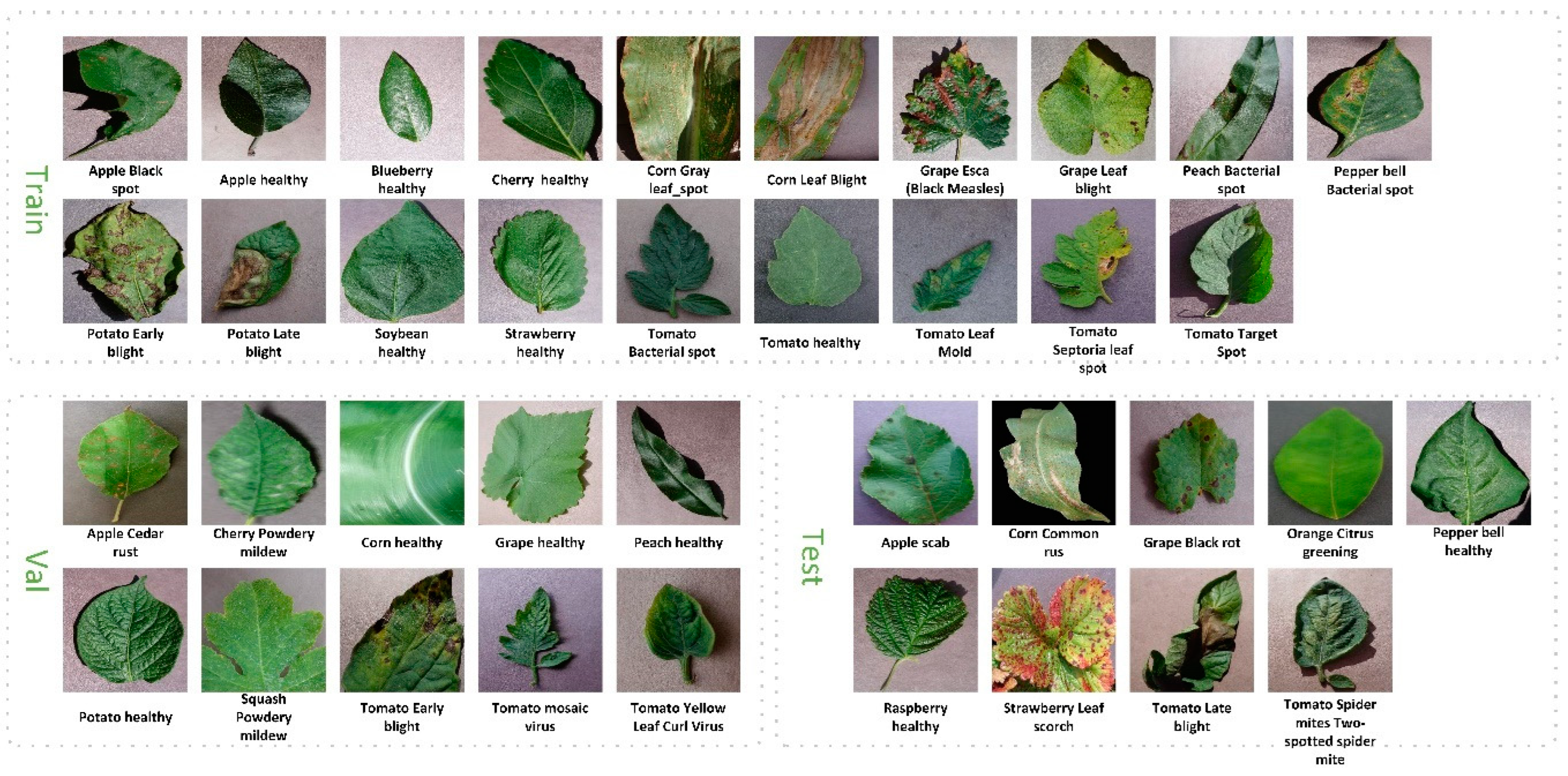
2.1. Materials
2.2. Problem Formulation
2.3. Methods
2.3.1. Baseline Framework for Meta-Learning
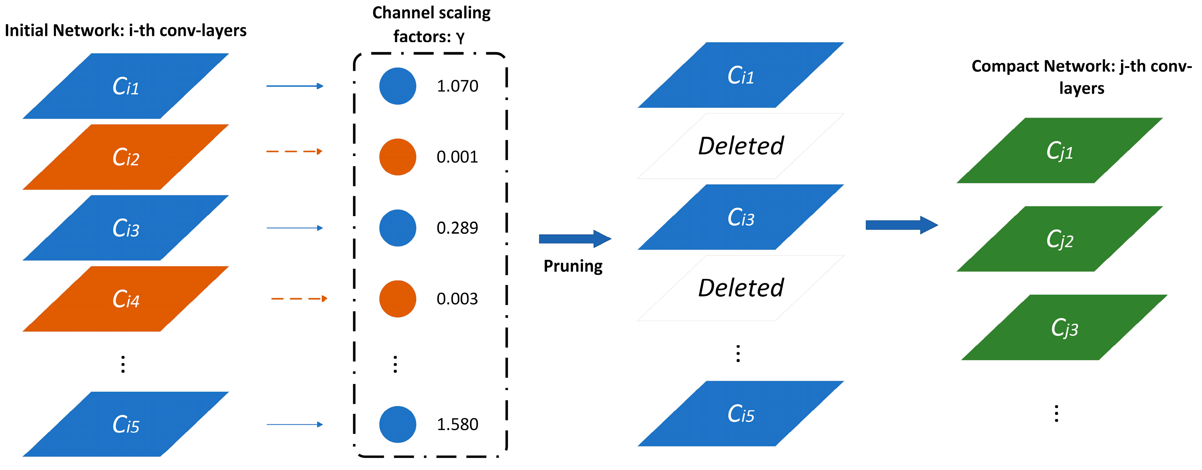
2.3.2. Slimming Network Pruning Algorithm
2.3.3. Indicators for Model Evaluation
3. Results
3.1. Data Setting
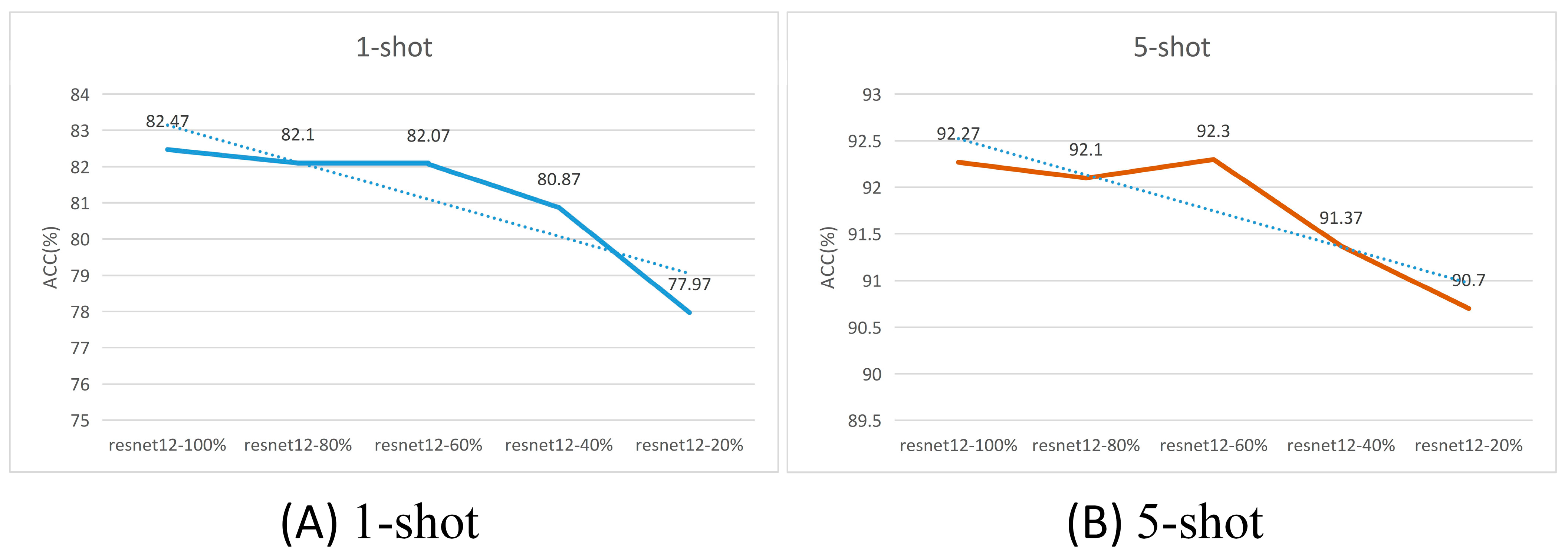
3.2. Effect of Pruning Coefficients on Model Performance
3.3. Effect of Pruning Strategy on Performance
3.4. Visualization of Loss Curves
3.5. K-Fold Cross-Validation
3.6. Comparison with Lightweight Networks
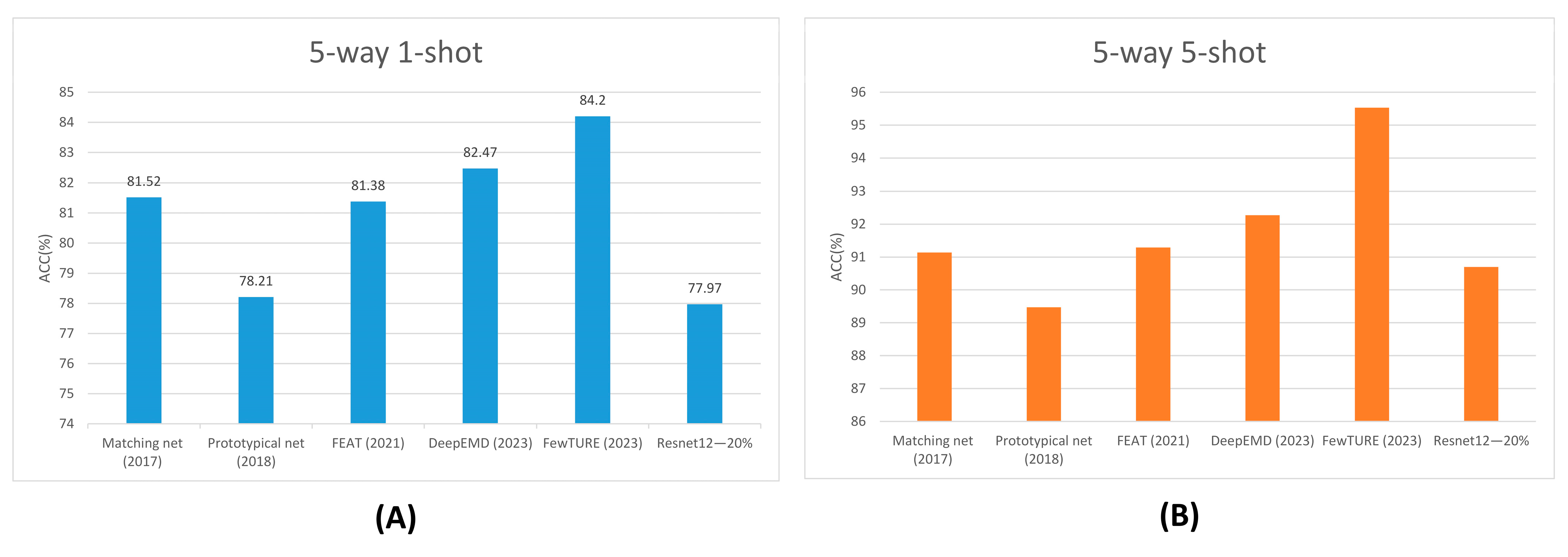
3.7. Comparison with Related Work
4. Discussion
4.1. Limitations of the Model and Future Work
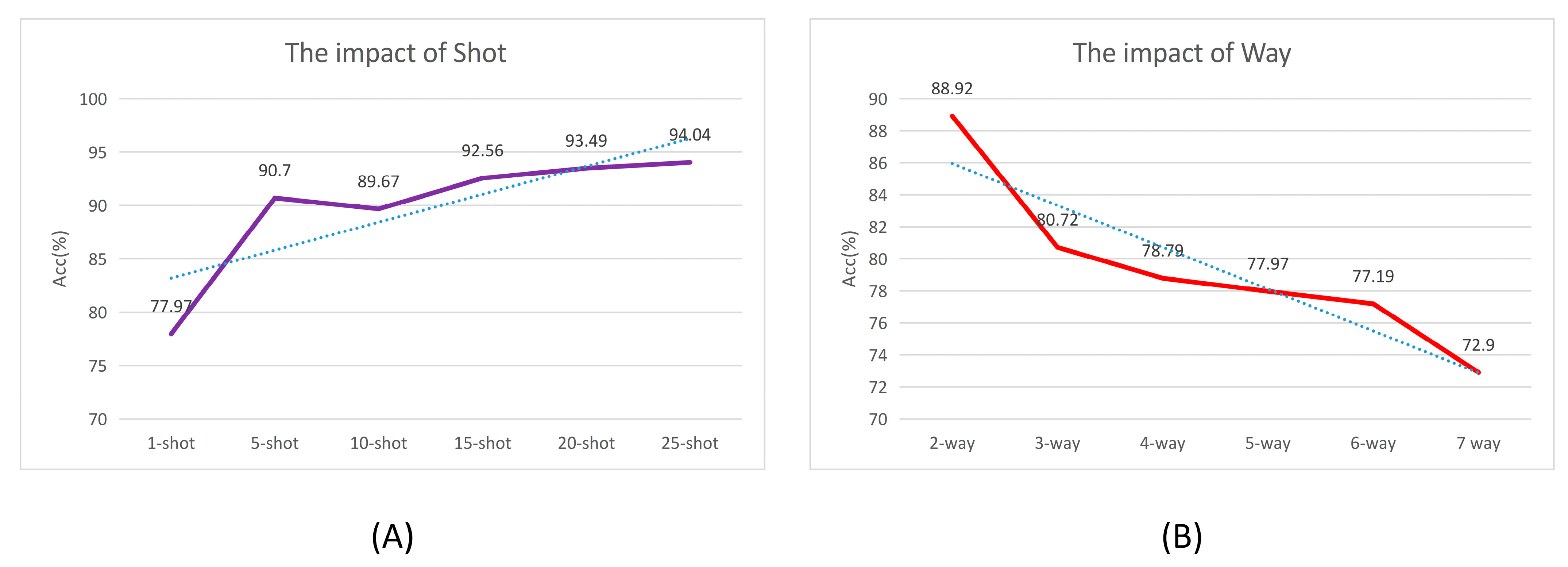
4.2. Effect of Way and Shot
5. Conclusions
Author Contributions
Funding
Data Availability Statement
Acknowledgments
Conflicts of Interest
References
- Strange, R.N.; Scott, P.R. Plant disease: A threat to global food security. Annu. Rev. Phytopathol. 2005, 43, 83–116. [Google Scholar] [CrossRef] [PubMed]
- Oerke, E.C.; Dehne, H.W. Safeguarding production—Losses in major crops and the role of crop protection. Crop Prot. 2004, 23, 275–285. [Google Scholar] [CrossRef]
- He, D.-c.; ZHAN, J.-s.; Xie, L.-h. Problems, challenges and future of plant disease management: From an ecological point of view. J. Integr. Agric. 2016, 15, 705–715. [Google Scholar] [CrossRef]
- Khakimov, A.; Salakhutdinov, I.; Omolikov, A.; Utaganov, S. Traditional and current-prospective methods of agricultural plant diseases detection: A review. IOP Conf. Ser. Earth Environ. Sci. 2022, 951, 012002. [Google Scholar] [CrossRef]
- Ma, J.; Du, K.; Zheng, F.; Zhang, L.; Gong, Z.; Sun, Z. A recognition method for cucumber diseases using leaf symptom images based on deep convolutional neural network. Comput. Electron. Agric. 2018, 154, 18–24. [Google Scholar] [CrossRef]
- Zhang, X.; Qiao, Y.; Meng, F.; Fan, C.; Zhang, M. Identification of Maize Leaf Diseases Using Improved Deep Convolutional Neural Networks. IEEE Access 2018, 6, 30370–30377. [Google Scholar] [CrossRef]
- Fuentes, A.; Yoon, S.; Kim, S.C.; Park, D.S. A Robust Deep-Learning-Based Detector for Real-Time Tomato Plant Diseases and Pests Recognition. Sensors 2017, 17, 2022. [Google Scholar] [CrossRef]
- Dhiman, P.; Kaur, A.; Balasaraswathi, V.R.; Gulzar, Y.; Alwan, A.A.; Hamid, Y. Image Acquisition, Preprocessing and Classification of Citrus Fruit Diseases: A Systematic Literature Review. Sustainability 2023, 15, 9643. [Google Scholar] [CrossRef]
- Long, M.S.; Ouyang, C.J.; Liu, H.; Fu, Q. Image recognition of Camellia oleifera diseases based on convolutional neural network & transfer learning. Trans. CSAE 2018, 34, 194–201. [Google Scholar] [CrossRef]
- Chen, J.; Ran, X. Deep learning with edge computing: A review. Proc. IEEE 2019, 107, 1655–1674. [Google Scholar] [CrossRef]
- Su, D.; Deng, Y.Z. Research progress and problems in crop disease image recognition. J. Tianjin Agric. Univ. 2023, 30, 75–79. [Google Scholar] [CrossRef]
- Véstias, M.P. Deep learning on edge: Challenges and trends. In Smart Systems Design, Applications, and Challenges; IGI Global: Hershey, PA, USA, 2020; pp. 23–42. [Google Scholar]
- Kamath, V.; Renuka, A. Deep learning based object detection for resource constrained devices: Systematic review, future trends and challenges ahead. Neurocomputing 2023, 531, 34–60. [Google Scholar] [CrossRef]
- Hu, G.S.; Wu, H.Y.; Zhang, Y.; Wan, M.Z. A low shot learning method for tea leaf’s disease identification. Comput. Electron. Agric. 2019, 163, 104852. [Google Scholar] [CrossRef]
- Chen, Y.P.; Pan, J.C.; Wu, Q.F. Apple leaf disease identification via improved CycleGAN and convolutional neural network. Soft Comput. 2023, 27, 9773–9786. [Google Scholar] [CrossRef]
- Cap, Q.H.; Uga, H.; Kagiwada, S.; Iyatomi, H. LeafGAN: An Effective Data Augmentation Method for Practical Plant Disease Diagnosis. IEEE Trans. Autom. Sci. Eng. 2022, 19, 1258–1267. [Google Scholar] [CrossRef]
- Pan, S.J.; Yang, Q.A. A Survey on Transfer Learning. IEEE Trans. Knowl. Data Eng. 2010, 22, 1345–1359. [Google Scholar] [CrossRef]
- Li, Z.J.; Xu, J.; Zeng, L.; Tie, J.; Yu, S. Small sample recognition method of tea disease based on improved DenseNet. Trans. CSAE 2022, 38, 182–190. [Google Scholar] [CrossRef]
- Yang, M.X.; Zhang, Y.G.; Liu, T. Corn disease recognition based on the Convolutional Neural Network with a small sampling size. Chin. J. Eco-Agric. 2020, 28, 1924–1931. [Google Scholar] [CrossRef]
- Xiao, W.; Quan, F. Research on plant disease identification based on few-shot learning. J. Chin. Agric. Mech. 2021, 42, 138–143. [Google Scholar]
- Lin, H.; Tse, R.; Tang, S.K.; Qiang, Z.P.; Pau, G. Few-shot learning approach with multi-scale feature fusion and attention for plant disease recognition. Front. Plant Sci. 2022, 13, 907916. [Google Scholar] [CrossRef]
- He, K.; Zhang, X.; Ren, S.; Sun, J. Deep residual learning for image recognition. In Proceedings of the IEEE Conference on Computer Vision and Pattern Recognition, Las Vegas, NV, USA, 27–30 June 2016; pp. 770–778. [Google Scholar]
- Zhang, C.; Cai, Y. DeepEMD: Differentiable Earth Mover’s Distance for Few-Shot Learning. arXiv 2023, arXiv:2003.06777v5. [Google Scholar] [CrossRef]
- Liu, Z.; Li, J.; Shen, Z.; Huang, G.; Yan, S.; Zhang, C. Learning efficient convolutional networks through network slimming. In Proceedings of the IEEE International Conference on Computer Vision, Venice, Italy, 22–29 October 2017; pp. 2736–2744. [Google Scholar]
- Huang, G.; Liu, Z.; Van Der Maaten, L.; Weinberger, K.Q. Densely connected convolutional networks. In Proceedings of the IEEE Conference on Computer Vision and Pattern Recognition, Honolulu, HI, USA, 21–26 July 2017; pp. 4700–4708. [Google Scholar]
- Ma, N.; Zhang, X.; Zheng, H.-T.; Sun, J. Shufflenet v2: Practical guidelines for efficient cnn architecture design. In Proceedings of the European Conference on Computer Vision (ECCV), Munich, Germany, 8–14 September 2018; pp. 116–131. [Google Scholar]
- Tan, M.; Le, Q. Efficientnet: Rethinking model scaling for convolutional neural networks. In Proceedings of the International Conference on Machine Learning, Long Beach, CA, USA, 9–15 June 2019; pp. 6105–6114. [Google Scholar]
- Sandler, M.; Howard, A.; Zhu, M.; Zhmoginov, A.; Chen, L.-C. Mobilenetv2: Inverted residuals and linear bottlenecks. In Proceedings of the IEEE Conference on Computer Vision and Pattern Recognition, Salt Lake City, UT, USA, 18–22 June 2018; pp. 4510–4520. [Google Scholar]
- Hughes, D.; Salathé, M. An open access repository of images on plant health to enable the development of mobile disease diagnostics. arXiv 2015, arXiv:1511.08060. [Google Scholar]
- Lake, B.M.; Salakhutdinov, R.; Tenenbaum, J.B. Human-level concept learning through probabilistic program induction. Science 2015, 350, 1332–1338. [Google Scholar] [CrossRef]
- Han, S.; Mao, H.; Dally, W.J. Deep compression: Compressing deep neural networks with pruning, trained quantization and huffman coding. arXiv 2015, arXiv:1510.00149. [Google Scholar]
- Santurkar, S.; Tsipras, D.; Ilyas, A.; Madry, A. How does batch normalization help optimization? In Advances in Neural Information Processing Systems; NeurIPS: San Diego, CA, USA, 2018; Volume 31. [Google Scholar]
- Yang, C.; Liu, H. Channel pruning based on convolutional neural network sensitivity. Neurocomputing 2022, 507, 97–106. [Google Scholar] [CrossRef]
- Molchanov, P.; Mallya, A.; Tyree, S.; Frosio, I.; Kautz, J. Importance estimation for neural network pruning. In Proceedings of the IEEE/CVF Conference on Computer Vision and Pattern Recognition, Long Beach, CA, USA, 15–20 June 2019; pp. 11264–11272. [Google Scholar]
- Finn, C.; Abbeel, P.; Levine, S. Model-agnostic meta-learning for fast adaptation of deep networks. In Proceedings of the International Conference on Machine Learning, Sydney, Australia, 6–11 August 2017; pp. 1126–1135. [Google Scholar]
- Guo, Y.; Yao, A.; Chen, Y. Dynamic network surgery for efficient dnns. In Advances in Neural Information Processing Systems; NeurIPS: San Diego, CA, USA, 2016; Volume 29. [Google Scholar]
- Diederik, P.K.; Ba, J. Adam: A method for stochastic optimization. arXiv 2014, arXiv:1412.6980. [Google Scholar]
- Yosinski, J.; Clune, J.; Bengio, Y.; Lipson, H. How transferable are features in deep neural networks? In Advances in Neural Information Processing Systems; NeurIPS: San Diego, CA, USA, 2014; Volume 27. [Google Scholar]
- Bengio, Y.; Grandvalet, Y. No unbiased estimator of the variance of k-fold cross-validation. In Advances in Neural Information Processing Systems; NeurIPS: San Diego, CA, USA, 2003; Volume 16. [Google Scholar]
- Gareth, J.; Daniela, W.; Trevor, H.; Robert, T. An Introduction to Statistical Learning: With Applications in R.; Spinger: Berlin/Heidelberg, Germany, 2013. [Google Scholar]
- Snell, J.; Swersky, K.; Zemel, R.S. Prototypical Networks for Few-shot Learning. arXiv 2017, arXiv:1703.05175. [Google Scholar]
- Vinyals, O.; Blundell, C. Matching Networks for One Shot Learning. arXiv 2017, arXiv:1606.04080v2. [Google Scholar]
- Ye, H.-J.; Hu, H.; Zhan, D.-C.; Sha, F. Few-shot learning via embedding adaptation with set-to-set functions. In Proceedings of the IEEE/CVF Conference on Computer Vision and Pattern Recognition, Seattle, WA, USA, 14–19 June 2020; pp. 8808–8817. [Google Scholar]
- Hiller, M.; Ma, R.; Harandi, M.; Drummond, T. Rethinking generalization in few-shot classification. In Advances in Neural Information Processing Systems; NeurIPS: San Diego, CA, USA, 2022; Volume 35, pp. 3582–3595. [Google Scholar]
- Barbedo, J.G.A. A review on the main challenges in automatic plant disease identification based on visible range images. Biosyst. Eng. 2016, 144, 52–60. [Google Scholar] [CrossRef]
- Alves-Júnior, M.; Alfenas-Zerbini, P.; Andrade, E.C.; Esposito, D.A.; Silva, F.N.; da Cruz, A.C.F.; Ventrella, M.C.; Otoni, W.C.; Zerbini, F.M. Synergism and negative interference during co-infection of tomato and Nicotiana benthamiana with two bipartite begomoviruses. Virology 2009, 387, 257–266. [Google Scholar] [CrossRef] [PubMed]
- Ferentinos, K.P. Deep learning models for plant disease detection and diagnosis. Comput. Electron. Agric. 2018, 145, 311–318. [Google Scholar] [CrossRef]
- Zhou, J.; Li, J.; Wang, C.; Wu, H.; Zhao, C.; Teng, G. Crop disease identification and interpretation method based on multimodal deep learning. Comput. Electron. Agric. 2021, 189, 106408. [Google Scholar] [CrossRef]
- Li, Y.; Chao, X. Semi-supervised few-shot learning approach for plant diseases recognition. Plant Methods 2021, 17, 68. [Google Scholar] [CrossRef]
- Nuthalapati, S.V.; Tunga, A. Multi-domain few-shot learning and dataset for agricultural applications. In Proceedings of the IEEE/CVF International Conference on Computer Vision, Montreal, BC, Canada, 11–17 October 2021; pp. 1399–1408. [Google Scholar]
- Yan, K.; Guo, X.; Ji, Z.; Zhou, X. Deep transfer learning for cross-species plant disease diagnosis adapting mixed subdomains. IEEE/ACM Trans. Comput. Biol. Bioinform. 2021, 20, 2555–2564. [Google Scholar] [CrossRef]
- Wang, J.; Jiang, J. Learning across tasks for zero-shot domain adaptation from a single source domain. IEEE Trans. Pattern Anal. Mach. Intell. 2021, 44, 6264–6279. [Google Scholar] [CrossRef]
- Ravi, S.; Larochelle, H. Optimization as a model for few-shot learning. In Proceedings of the International Conference on Learning Representations, San Juan, Puerto Rico, 2–4 May 2016. [Google Scholar]


| Species | Class Numbers | Class Name | Number in PV |
|---|---|---|---|
| Apple | 4 | Apple scab, Black rot, Cedar apple rust, Healthy | 3174 |
| Blueberry | 1 | Healthy | 1502 |
| Cherry | 2 | Healthy, Powdery mildew | 1905 |
| Corn | 4 | Cercospora leaf spot, Gray leaf spot, Common rust, Northern leaf blight, Healthy | 3852 |
| Grape | 4 | Black rot, Black measles, Healthy, Leaf blight | 3862 |
| Orange | 1 | Haunglongbing | 5507 |
| Peach | 2 | Bacterial spot, Healthy | 2657 |
| Pepper | 2 | Bell bacterial spot, Bell healthy | 2473 |
| Potato | 3 | Early blight, Healthy, Late blight | 2152 |
| Raspberry | 1 | Healthy | 371 |
| Soybean | 1 | Healthy | 5089 |
| Squash | 1 | Powdert mildew | 1835 |
| Strawberry | 2 | Healthy, Leaf scorch | 1565 |
| Tomato | 10 | Bacterial spot, Early blight, Healthy, Late blight, Leaf mold, Septoria leaf spot, Spider mite, Two-spotted spider mite, Target spot, Tomato mosaic virus (TMOV), Yellow leaf curl virus (YLCV) | 18,159 |
| Network | Training Stage | Paramars (M) | Macs (G) | 5-way 1-shot | 5-way 5-shot | ||
|---|---|---|---|---|---|---|---|
| Acc (%) | 95% MSE | Acc (%) | 95% MSE | ||||
| Resnet12—80% | A | 0.49 | 0.14 | 77.97 | 1.46 | 90.70 | 1.02 |
| Resnet12—60% | A | 1.99 | 0.56 | 80.87 | 1.32 | 91.37 | 0.98 |
| Resnet12—40% | A | 4.47 | 1.27 | 82.07 | 1.30 | 92.30 | 0.90 |
| Resnet12—20% | A | 7.95 | 2.25 | 82.10 | 1.31 | 92.10 | 0.93 |
| Resnet12—0% | A | 12.42 | 3.52 | 82.47 | 1.30 | 92.27 | 0.91 |
| Network | Training Stage | 5-way 1-shot | 5-way 5-shot | ||
|---|---|---|---|---|---|
| Acc (%) | 95% MSE | Acc (%) | 95% MSE | ||
| Resnet12—80% | A | 77.97 | 1.46 | 90.70 | 1.02 |
| Resnet12—60% | A | 80.87 | 1.32 | 91.37 | 0.98 |
| Resnet12—40% | A | 82.07 | 1.30 | 92.30 | 0.90 |
| Resnet12—20% | A | 82.10 | 1.31 | 92.10 | 0.93 |
| Resnet12—80% | B | 55.53 | 1.72 | 65.77 | 1.65 |
| Resnet12—60% | B | 60.70 | 1.69 | 69.13 | 1.55 |
| Resnet12—40% | B | 71.00 | 1.53 | 81.73 | 1.37 |
| Resnet12—20% | B | 79.33 | 1.42 | 88.60 | 1.12 |
| Network | Fold | 5-way 1-shot | 5-way 5-shot | ||
|---|---|---|---|---|---|
| Acc (%) | 95% MSE | Acc (%) | 95% MSE | ||
| Resnet12—20% | 1st fold | 73.00 | 1.54 | 89.40 | 1.07 |
| Resnet12—20% | 2nd fold | 76.70 | 1.32 | 90.37 | 1.07 |
| Resnet12—20% | 3th fold | 79.77 | 1.41 | 87.47 | 1.19 |
| Resnet12—20% | 4th fold | 77.77 | 1.42 | 87.43 | 1.15 |
| Resnet12—20% | 5th fold | 78.60 | 1.39 | 89.63 | 1.06 |
| Resnet12—20% | AVG | 77.17 | 1.42 | 88.86 | 1.11 |
| Network | Paramars (M) | Macs (G) | 5-way 1-shot | 5-way 1-shot | ||
|---|---|---|---|---|---|---|
| Acc(%) | 95% MSE | Acc(%) | 95% MSE | |||
| Shufflenetv2 | 1.99 | 0.03 | 73.60 | 1.55 | 87.70 | 1.18 |
| Mobilenetv2 | 3.50 | 0.05 | 72.67 | 1.45 | 85.90 | 1.27 |
| Mobilenetv3 | 5.76 | 0.05 | 67.60 | 1.62 | 82.30 | 1.37 |
| EfficientNet | 2.82 | 0.03 | 73.60 | 1.50 | 85.70 | 1.25 |
| Densenet40 | 0.61 | 0.82 | 79.63 | 1.41 | 94.40 | 0.80 |
| Resnet12 | 12.42 | 3.52 | 82.47 | 1.30 | 92.27 | 0.91 |
| Resnet12—80% | 0.49 | 0.14 | 77.97 | 1.46 | 90.70 | 1.02 |
| Method | 5-way 1-shot | 5-way 5-shot | ||
|---|---|---|---|---|
| Acc (%) | 95% MSE | Acc (%) | 95% MSE | |
| Matching net (2017) | 81.52 | 0.01 | 91.14 | 0.01 |
| Prototypical net (2018) | 78.21 | 1.56 | 89.47 | 1.06 |
| FEAT (2021) | 81.38 | 1.35 | 91.29 | 0.96 |
| DeepEMD (2023) | 82.47 | 1.30 | 92.27 | 0.91 |
| FewTURE (2023) | 84.20 | 1.21 | 95.53 | 0.74 |
| Resnet12—20% | 77.97 | 1.46 | 90.70 | 1.02 |
Disclaimer/Publisher’s Note: The statements, opinions and data contained in all publications are solely those of the individual author(s) and contributor(s) and not of MDPI and/or the editor(s). MDPI and/or the editor(s) disclaim responsibility for any injury to people or property resulting from any ideas, methods, instructions or products referred to in the content. |
© 2024 by the authors. Licensee MDPI, Basel, Switzerland. This article is an open access article distributed under the terms and conditions of the Creative Commons Attribution (CC BY) license (https://creativecommons.org/licenses/by/4.0/).
Share and Cite
Yan, W.; Feng, Q.; Yang, S.; Zhang, J.; Yang, W. Prune-FSL: Pruning-Based Lightweight Few-Shot Learning for Plant Disease Identification. Agronomy 2024, 14, 1878. https://doi.org/10.3390/agronomy14091878
Yan W, Feng Q, Yang S, Zhang J, Yang W. Prune-FSL: Pruning-Based Lightweight Few-Shot Learning for Plant Disease Identification. Agronomy. 2024; 14(9):1878. https://doi.org/10.3390/agronomy14091878
Chicago/Turabian StyleYan, Wenbo, Quan Feng, Sen Yang, Jianhua Zhang, and Wanxia Yang. 2024. "Prune-FSL: Pruning-Based Lightweight Few-Shot Learning for Plant Disease Identification" Agronomy 14, no. 9: 1878. https://doi.org/10.3390/agronomy14091878