
Monitoring of Soybean Bacterial Blight Disease Using Drone-Mounted Multispectral Imaging: A Case Study in Northeast China

Abstract
:1. Introduction
2. Materials and Methods
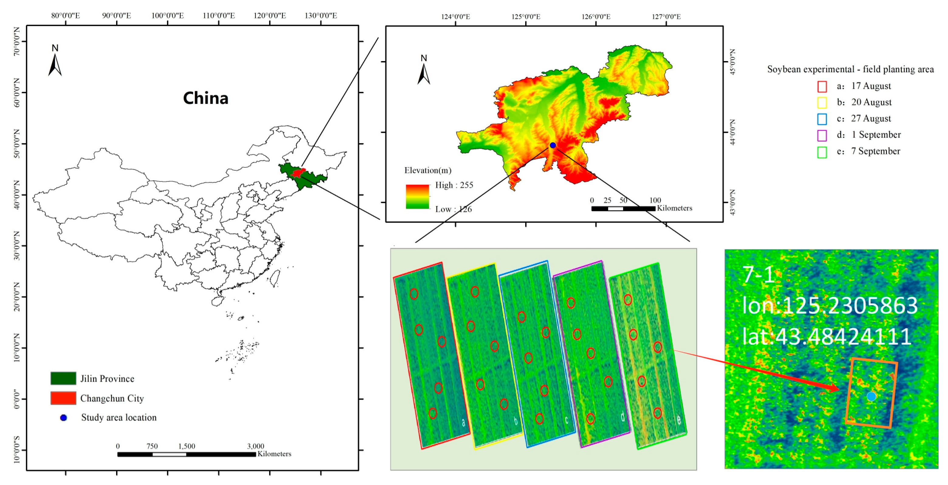
2.1. Overview of the Test Area
2.2. Establishment of Sampling Points
2.3. Pathogen Culture and Inoculation
2.3.1. Preparation of Bacterial Suspensions
2.3.2. Inoculations of Pathogens in Field
2.4. Ground Data Acquisition
2.5. UAV Image Acquisition and Preprocessing
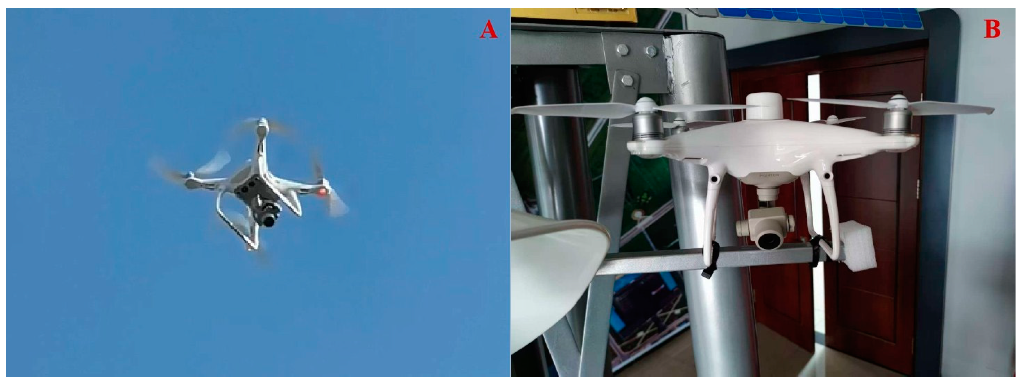
2.5.1. UAV Multispectral Remote Sensing Platform
2.5.2. Monitoring Method
Monitoring Time
Image Spectral Bands
Vegetation Index
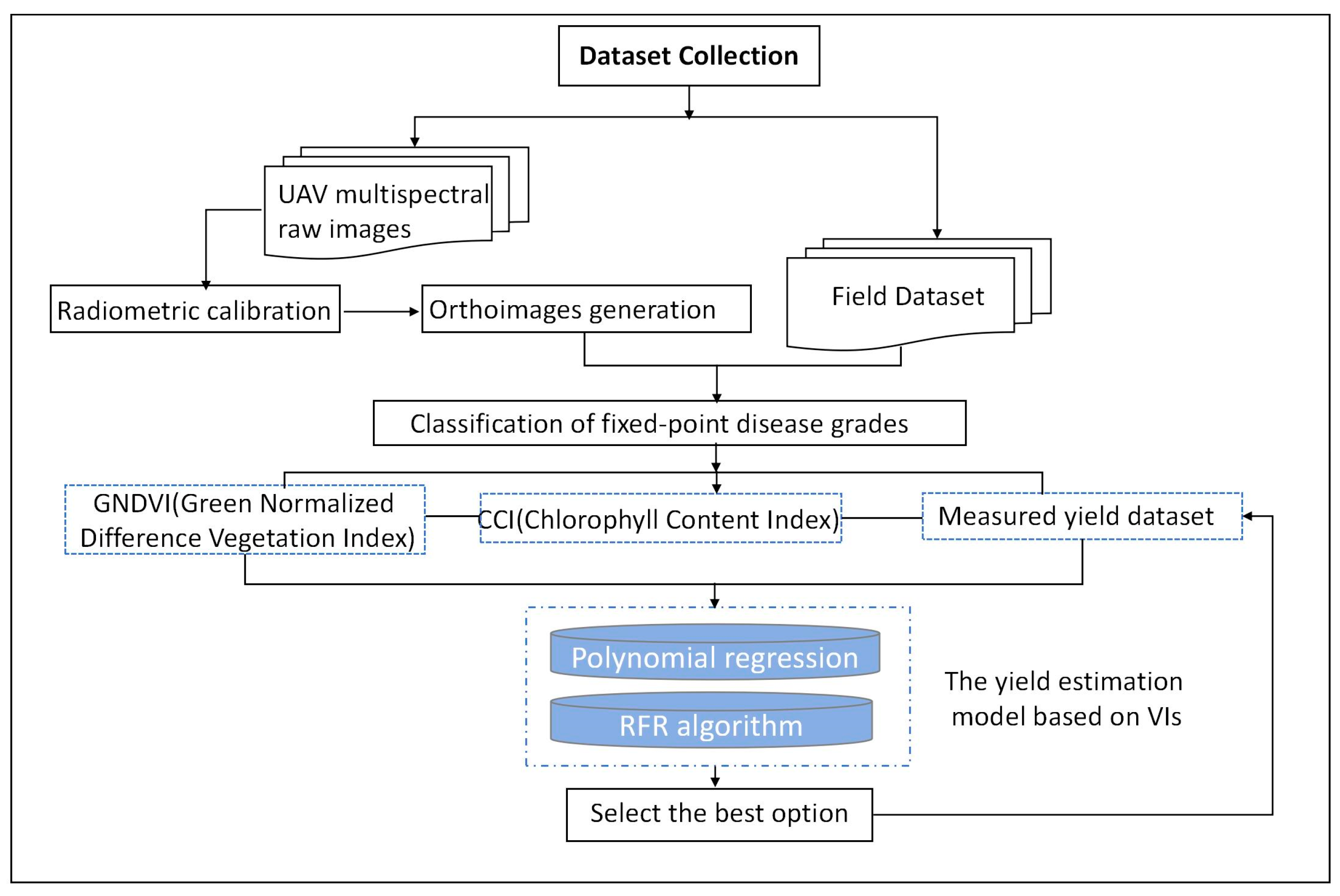
2.6. Soybean Yield Estimation
2.7. Statistical Analysis
3. Results
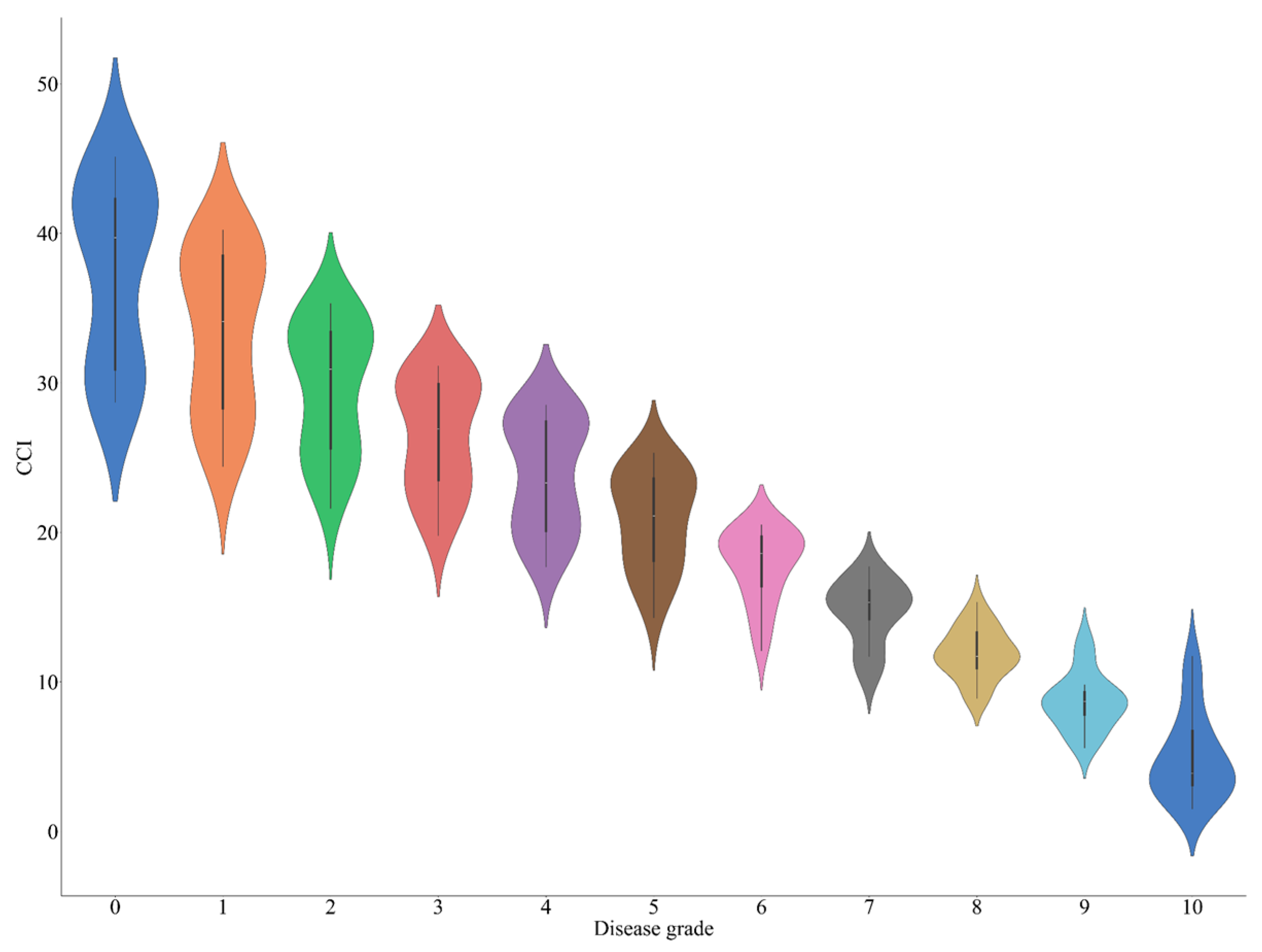
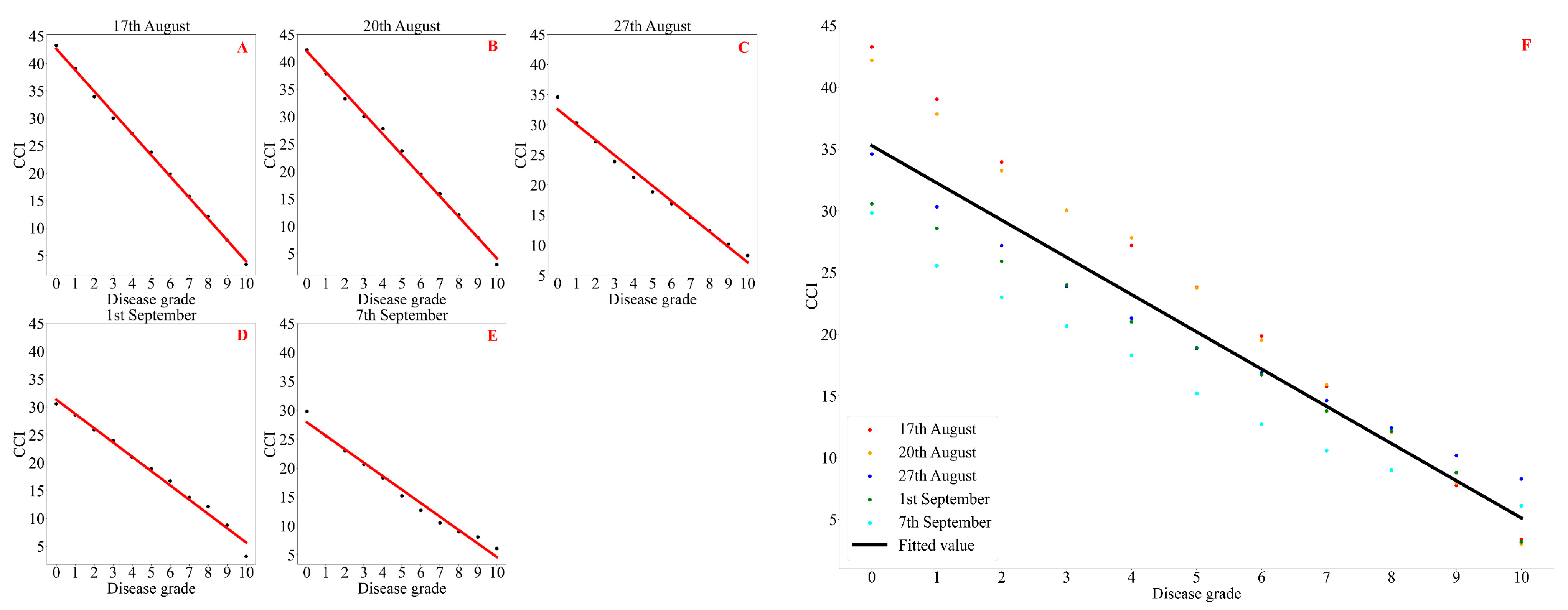
3.1. Correlation Analysis Between Soybean CCI and Disease Grades of Soybean Bacterial Blight
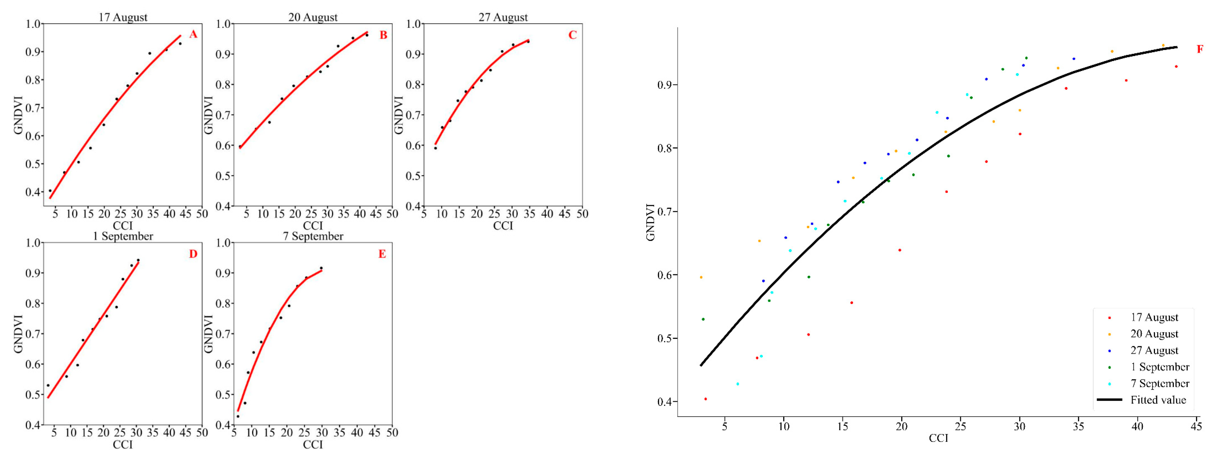
3.2. Correlation Analysis of Soybean CCI and GNDVI
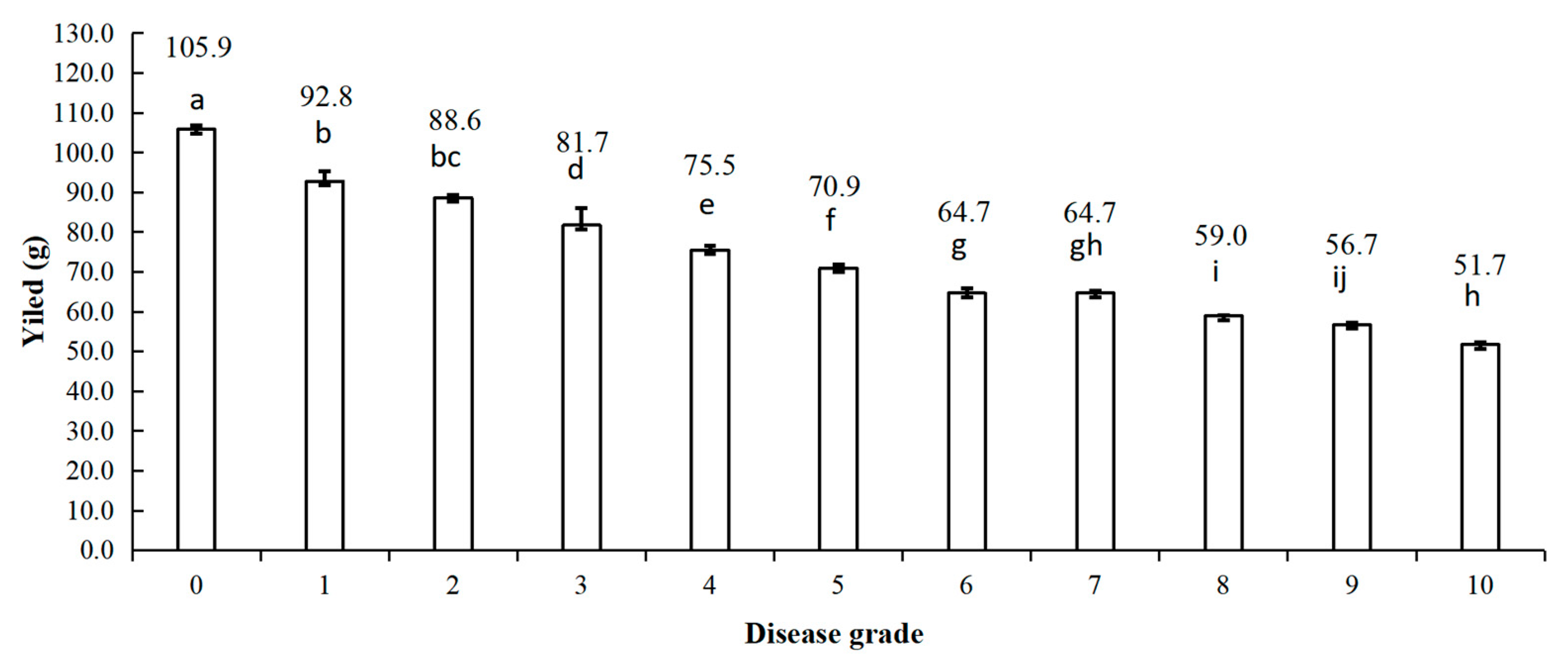
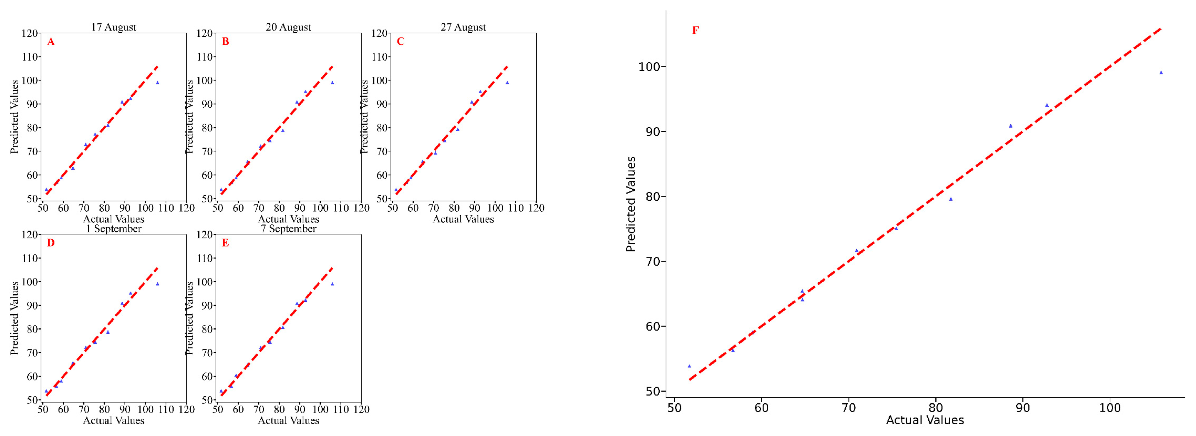
3.3. Estimation of Soybean Yields
4. Discussion
5. Conclusions
Supplementary Materials
Author Contributions
Funding
Data Availability Statement
Acknowledgments
Conflicts of Interest
References
- Bandara, A.Y.; Weerasooriya, D.K.; Bradley, C.A.; Allen, T.W.; Esker, P.D. Dissecting the economic impact of soybean diseases in the United States over two decades. PLoS ONE 2020, 15, e0231141. [Google Scholar] [CrossRef] [PubMed]
- Tarakanov, R.; Shagdarova, B.; Lyalina, T.; Zhuikova, Y.; Il’ina, A.; Dzhalilov, F.; Varlamov, V. Protective properties of copper-loaded chitosan nanoparticles against soybean pathogens Pseudomonas savastanoi pv. glycinea and Curtobacterium flaccumfaciens pv. flaccumfaciens. Polymers 2023, 15, 1100. [Google Scholar] [CrossRef]
- El-Esawi, M.A.; Ali, H.M.; Hatamleh, A.A.; Al-Dosary, M.A.; El-Ballat, E.M. Multi-functional PGPR Serratia liquefaciens confers enhanced resistance to lead stress and bacterial blight in soybean (Glycine max L.). Curr. Plant Biol. 2024, 40, 100403. [Google Scholar] [CrossRef]
- Feng, J. Recent advances in taxonomy of plant pathogenic bacteria. J. Integr. Agric. 2017, 50, 2305–2314, (In Chinese with English Abstract). [Google Scholar] [CrossRef]
- Wang, C.; Linderholm, H.W.; Song, Y.; Wang, F.; Liu, Y.; Tian, J.; Xu, J.; Song, Y.; Ren, G. Impacts of drought on maize and soybean production in Northeast China during the past five decades. Int. J. Environ. Res. Public Health 2020, 17, 2459. [Google Scholar] [CrossRef]
- Ye, W.W.; Liu, W.C.; Wang, Y.C. Occurrence status and whole-process green control technologies for soybean diseases and pests in China. J. Plant Prot. 2023, 50, 265–273, (In Chinese with English Abstract). [Google Scholar] [CrossRef]
- Surbhi, K.; Singh, K.; Aravind, T.; Bhatt, P.; Jeena, H.; Rakhonde, G. GIS-based survey and molecular detection of bacterial blight of soybean in Sub-Himalayan Ranges of Uttarakhand, India. Trop. Plant Pathol. 2023, 48, 332–346. [Google Scholar] [CrossRef]
- Zhao, F.Z.; Wang, Y.A.; Cheng, W.; Antwi-Boasiako, A.; Yan, W.K.; Zhang, C.T.; Gao, X.W.; Kong, J.J.; Liu, W.S.; Zhao, T.J. Genome-wide association study of bacterial blight resistance in soybean. Plant Dis. 2025, 109, 341–351. [Google Scholar] [CrossRef]
- Zhang, J.H.; Gao, J.; Yuan, M.L.; Li, Y. Studies on the distribution of physiological races of Pseudomonas syringae pv. glycinea. J. Jilin Agric. Univ. 2003, 25, 24–26, (In Chinese with English Abstract). [Google Scholar] [CrossRef]
- Zhang, J.H.; Gao, J.; Yuan, M.L. Identification of physiological races of Pseudomonas syringae pv. glycinea in Jilin province. J. Jilin Agric. Univ. 1993, 15, 24–27+105, (In Chinese with English Abstract). [Google Scholar] [CrossRef]
- Jagtap, P.G.; Dhopte, S.B.; Dey, U. Evaluation of different antibacterial antibiotics against bacterial blight of soybean caused by Pseudomonas syringae pv. glycinea under field conditions. Ind. Phytopathol. 2013, 66, 411–412. [Google Scholar]
- Wang, X.Y.; Li, Y.; Pan, T.; Zhang, Z.G.; Qu, J.Q.; Sun, Y.Z.; Zhao, H.J.; Miao, L.X.; Hu, Z.B.; Zhao, Z.M.; et al. Diagnosis of soybean bacterial blight progress stage based on deep learning in the context of data-deficient. Comput. Electron. Agric. 2023, 212, 108170. [Google Scholar] [CrossRef]
- Sotelo, J.P.; Rovey, M.F.P.; María, E.C.; Moliva, M.V.; Oliva, M.D.L.M. Characterization of Pseudomonas syringae strains associated with soybean bacterial blight and in vitro inhibitory effect of oregano and thyme essential oils. Physiol. Mol. Plant Pathol. 2023, 128, 102133. [Google Scholar] [CrossRef]
- Rahman, M.H.; Sejan, M.A.S.; Aziz, M.A.; Tabassum, R.; Baik, J.-I.; Song, H.-K. A comprehensive survey of unmanned aerial vehicles detection and classification using machine learning approach: Challenges, solutions, and future directions. Remote Sens. 2024, 16, 879. [Google Scholar] [CrossRef]
- Mukherjee, A.; Misra, S.; Raghuwanshi, N.S. A survey of unmanned aerial sensing solutions in precision agriculture. J. Netw. Comput. Appl. 2019, 148, 102461. [Google Scholar] [CrossRef]
- Huang, Y.B.; Thomson, S.J.; Brand, H.J.; Reddy, K.N. Development and evaluation of low-altitude remote sensing systems for crop production management. Int. J. Agric. Biol. Eng. 2016, 9, 1–11. [Google Scholar] [CrossRef]
- Yuan, J.; Zhang, Y.; Zheng, Z.; Yao, W.; Wang, W.; Guo, L. Grain crop yield prediction using machine learning based on UAV remote sensing: A systematic literature review. Drones 2024, 8, 559. [Google Scholar] [CrossRef]
- Zahra, A.; Qureshi, R.; Sajjad, M.; Sadak, F.; Nawaz, M.; Khan, H.A.; Uzair, M. Current advances in imaging spectroscopy and its state-of-the-art applications. Expert Syst. Appl. 2024, 238, 122172. [Google Scholar] [CrossRef]
- Hou, Y.; Bao, H.; Rimi, T.I.; Zhang, S.; Han, B.; Wang, Y.; Yu, Z.; Chen, J.; Gao, H.; Zhao, Z.; et al. Rice quality and yield prediction based on multi-source indicators at different periods. Plants 2025, 14, 424. [Google Scholar] [CrossRef]
- Yu, Y.; Li, C.; Shen, W.; Yan, L.; Zheng, X.; Yao, Z.; Cui, S.; Cui, C.; Hu, Y.; Yang, M. Correlation study between canopy temperature (CT) and wheat yield and quality based on infrared imaging camera. Plants 2025, 14, 411. [Google Scholar] [CrossRef]
- Sukhova, E.; Zolin, Y.; Popova, A.; Grebneva, K.; Yudina, L.; Sukhov, V. Broadband normalized difference reflectance indices and the normalized red–green index as a measure of drought in wheat and pea plants. Plants 2025, 14, 71. [Google Scholar] [CrossRef] [PubMed]
- Shrivastava, S.; Singh, K.S.; Hooda, S.D. Color sensing and image processing-based automatic soybean plant foliar disease severity detection and estimation. Multimed. Tools Appl. 2015, 74, 11467–11484. [Google Scholar] [CrossRef]
- Marston, Z.P.D.; Cira, T.M.; Hodgson, E.W.; Knight, J.F.; MacRae, I.V.; Koch, R.L. Detection of stress induced by soybean aphid (Hemiptera: Aphididae) using multispectral imagery from unmanned aerial vehicles. J. Econ. Entomol. 2020, 113, 779–786. [Google Scholar] [CrossRef]
- Mignoni, M.E.; Honorato, A.; Kunst, R.; Righi, R.; Massuquetti, A. Soybean images dataset for caterpillar and Diabrotica speciosa pest detection and classification. Data Brief 2022, 40, 107756. [Google Scholar] [CrossRef] [PubMed]
- Yamamoto, S.; Nomoto, S.; Hashimoto, N.; Maki, M.; Hongo, C.; Shiraiwa, T.; Homma, K. Monitoring spatial and time-series variations in red crown rot damage of soybean in farmer fields based on UAV remote sensing. Plant. Prod. Sci. 2023, 26, 36–47. [Google Scholar] [CrossRef]
- Tetila, E.C.; Machado, B.B.; de Souza Belete, N.A.; Guimaraes, D.A.; Pistori, H. Identification of soybean foliar diseases using unmanned aerial vehicle images. IEEE Geosci. Remote Sens. Lett. 2017, 14, 2190–2194. [Google Scholar] [CrossRef]
- Nagasubramanian, K.; Jones, S.; Singh, A.K.; Sarkar, S.; Singh, A.; Ganapathysubramanian, B. Plant disease identification using explainable 3D deep learning on hyperspectral images. Plant Methods 2019, 15, 98. [Google Scholar] [CrossRef]
- Liu, S.; Yu, H.-Y.; Sui, Y.-Y.; Kong, L.-J.; Yu, Z.-D.; Guo, J.-J.; Qiao, J. Hyperspectral data analysis for classification of soybean leaf diseases. Spectrosc. Spectr. Anal. 2023, 43, 1550–1555. [Google Scholar] [CrossRef]
- Afolabi, C.G.; Salihu, S.; Shokalu, O. Screening of soybean [Glycine max (L.) merrill] lines for reaction to natural field infection and resistant against bacteria foliar diseases. Arch. Phytopathol. Plant Protect. 2023, 56, 269–283. [Google Scholar] [CrossRef]
- Brown, M.T.; Mueller, D.S.; Kandel, Y.R.; Telenko, D.E.P. Influence of integrated management strategies on soybean sudden death syndrome (SDS) root infection, foliar symptoms, yield and net returns. Pathogens 2023, 12, 913. [Google Scholar] [CrossRef]
- Ravelombola, W.S.; Qin, J.; Shi, A.; Nice, L.; Bao, Y.; Lorenz, A.; Orf, J.H.; Young, N.D.; Chen, S. Genome-wide association study and genomic selection for soybean chlorophyll content associated with soybean cyst nematode tolerance. BMC Genom. 2019, 20, 904. [Google Scholar] [CrossRef] [PubMed]
- Yang, C.; Yang, G.; Wang, H.; Li, S.; Zhang, J.; Pan, D.; Ren, P.; Feng, H.; Li, H. Identifying key traits for screening high-yield soybean varieties by combining UAV-based and field phenotyping. Remote Sens. 2025, 17, 690. [Google Scholar] [CrossRef]
- Maimaitijiang, M.; Sagan, V.; Sidike, P.; Hartling, S.; Esposito, F.; Fritschi, F.B. Soybean yield prediction from UAV using multimodal data fusion and deep learning. Remote Sens. Environ. 2020, 237, 111599. [Google Scholar] [CrossRef]
- Huang, W.J.; Huang, M.Y.; Liu, L.Y.; Wang, J.H.; Zhao, C.J.; Wang, J.D. Inversion of the severity of winter wheat yellow rust using proper hyper spectral index. Trans. Chin. Soc. Agric. Eng. 2005, 21, 97–103. [Google Scholar]
- Shi, W.; Li, Y.; Zhang, W.; Yu, C.; Zhao, C.; Qiu, J. Monitoring and zoning soybean maturity using UAV remote sensing. Ind. Crops Prod. 2024, 222, 119470. [Google Scholar] [CrossRef]
- Jia, S.; Cui, M.; Chen, L.; Guo, S.; Zhang, H.; Bai, Z.; Li, Y.; Deng, L.; Li, F.; Zhang, W. Soybean water monitoring and water demand prediction in arid region based on UAV multispectral data. Agronomy 2025, 15, 88. [Google Scholar] [CrossRef]
- Kyratzis, A.C.; Skarlatos, D.P.; Menexes, G.C.; Vamvakousis, V.F.; Katsiotis, A. Assessment of vegetation indices derived by UAV imagery for durum wheat phenotyping under a water limited and heat stressed mediterranean environment. Front. Plant Sci. 2017, 8, 1114. [Google Scholar] [CrossRef]
- Tiruneh, G.A.; Meshesha, D.T.; Adgo, E.; Tsunekawa, A.; Haregeweyn, N.; Fenta, A.A.; Reichert, J.M. A leaf reflectance-based crop yield modeling in Northwest Ethiopia. PLoS ONE 2022, 17, e0269791. [Google Scholar] [CrossRef]


| Band | Wavelength Range (nm) |
|---|---|
| Blue | 450 ± 16 |
| Green | 560 ± 16 |
| Red | 650 ± 16 |
| Red Edge | 730 ± 16 |
| Near-Infrared | 840 ± 26 |
| Vegetation Index | Equation |
|---|---|
| Normalized Red Light (R) | R/(R + G + B) |
| Normalized Green Light (G) | G/(R + G + B) |
| Normalized Blue Light (B) | B/(R + G + B) |
| Green Normalized Vegetation Index (GNDVI) | (NIR − G)/(NIR + G) |
| Disease Grade | 17 August (Podding Stage to Beginning of Grain Stage) | 20 August (Beginning of Grain Stage to Full Grain Stage) | 27 August (Full Grain Stage to First Maturity Stage) | 1 September (First Maturity Stage to Full Grain Stage) | 7 September (Full Grain Stage) |
|---|---|---|---|---|---|
| 0 | 43.28 ± 0.72 a | 42.18 ± 0.82 a | 35.74 ± 2.06 a | 30.57 ± 1.04 a | 29.80 ± 1.10 a |
| 1 | 39.04 ± 0.45 b | 37.84 ± 0.59 b | 31.12 ± 1.32 b | 28.57 ± 0.93 b | 25.55 ± 1.15 b |
| 2 | 33.94 ± 0.53 c | 33.26 ± 0.29 c | 27.88 ± 1.26 c | 25.90 ± 0.36 c | 23.00 ± 1.40 c |
| 3 | 30.04 ± 0.43 d | 30.02 ± 0.36 d | 24.50 ± 0.80 d | 23.97 ± 0.47 d | 20.65 ± 0.85 d |
| 4 | 27.18 ± 0.24 e | 27.80 ± 0.23 e | 21.70 ± 0.74 e | 21.00 ± 0.80 e | 18.30 ± 0.60 e |
| 5 | 23.80 ± 0.34 f | 23.74 ± 0.48 f | 19.28 ± 0.73 f | 18.90 ± 0.78 f | 15.20 ± 0.90 f |
| 6 | 19.84 ± 0.18 g | 19.52 ± 0.32 g | 17.18 ± 0.88 g | 16.73 ± 0.58 g | 12.70 ± 0.60 g |
| 7 | 15.76 ± 0.43 h | 15.90 ± 0.45 h | 14.70 ± 1.17 h | 13.77 ± 1.07 h | 10.55 ± 0.35 h |
| 8 | 12.10 ± 0.45 i | 12.06 ± 0.43 i | 12.64 ± 1.15 i | 12.13 ± 0.72 i | 9.00 ± 0.10 i |
| 9 | 7.74 ± 0.70 j | 7.94 ± 0.76 j | 10.36 ± 1.17 j | 8.77 ± 0.29 j | 8.10 ± 0.20 j |
| 10 | 3.38 ± 0.68 k | 3.00 ± 0.42 k | 8.52 ± 1.43 k | 3.17 ± 0.35 k | 6.10 ± 0.80 k |
| Observation Date | Fitting Model | R2 | F | p | mae | mse | rmse |
|---|---|---|---|---|---|---|---|
| 17 August (podding stage to beginning of grain stage) | y = −3.75x + 45.71 | 0.998 | 3801.137 | 3.918 × 10⁻¹³ | 0.460 | 0.305 | 0.552 |
| 20 August (beginning of grain stage to full grain stage) | y = −3.78x + 41.92 | 0.997 | 2901.179 | 1.318 × 10⁻¹² | 0.561 | 0.443 | 0.665 |
| 27 August (full grain stage to first maturity stage) | y = −2.68x + 35.26 | 0.988 | 716.605 | 6.854 × 10⁻¹⁰ | 0.741 | 0.852 | 0.923 |
| 1 September (first maturity stage to full grain stage) | y = −2.87x + 37.51 | 0.982 | 484.379 | 3.898 × 10⁻⁹ | 0.691 | 0.916 | 0.957 |
| 7 September (full grain stage) | y = −2.57x + 31.65 | 0.980 | 435.187 | 6.258 × 10⁻⁹ | 0.819 | 1.015 | 1.000 |
| Disease Grade | GNDVI | GNDVI_Sd | GNDVI_Range | ||||
|---|---|---|---|---|---|---|---|
| 17 August (Podding Stage to Beginning of Grain Stage) | 20 August (Beginning of Grain Stage to Full Grain Stage) | 27 August (Full Grain Stage to First Maturity Stage) | 1 September (First Maturity Stage to Full Grain Stage) | 7 September (Full Grain Stage) | 17th August to 7th September (Podding Stage to Full Grain Stage) | ||
| 0 | 0.9287 | 0.9621 | 0.9408 | 0.9420 | 0.9160 | 0.938 ± 0.017 | 0.9621~0.9160 |
| 1 | 0.9067 | 0.9525 | 0.9305 | 0.9243 | 0.8843 | 0.920 ± 0.026 | 0.9525~0.8843 |
| 2 | 0.8222 | 0.8596 | 0.8471 | 0.7874 | 0.7916 | 0.822 ± 0.032 | 0.8596~0.7874 |
| 3 | 0.7786 | 0.8418 | 0.8128 | 0.7578 | 0.7523 | 0.789 ± 0.038 | 0.8418~0.7523 |
| 4 | 0.7311 | 0.8256 | 0.7904 | 0.7480 | 0.7163 | 0.762 ± 0.045 | 0.8256~0.7163 |
| 5 | 0.6390 | 0.7953 | 0.7764 | 0.7146 | 0.6726 | 0.720 ± 0.066 | 0.7953~0.6390 |
| 6 | 0.5560 | 0.7530 | 0.7465 | 0.6788 | 0.6382 | 0.675 ± 0.082 | 0.7465~0.5560 |
| 7 | 0.5057 | 0.6754 | 0.6806 | 0.5965 | 0.5721 | 0.606 ± 0.074 | 0.6806~0.5057 |
| 8 | 0.4689 | 0.6535 | 0.6586 | 0.5592 | 0.4717 | 0.562 ± 0.093 | 0.6586~0.4689 |
| 9 | 0.4041 | 0.5961 | 0.5903 | 0.5299 | 0.4278 | 0.510 ± 0.090 | 0.5961~0.4041 |
| 10 | 0.3621 | 0.5270 | 0.5335 | 0.4569 | 0.3459 | 0.445 ± 0.089 | 0.5335~0.3459 |
| Observation Date | Polynomial Regression | Random Forest Regression | ||||||
|---|---|---|---|---|---|---|---|---|
| Fitting Model | R2 | F | p | mae | mse | rmse | R2 | |
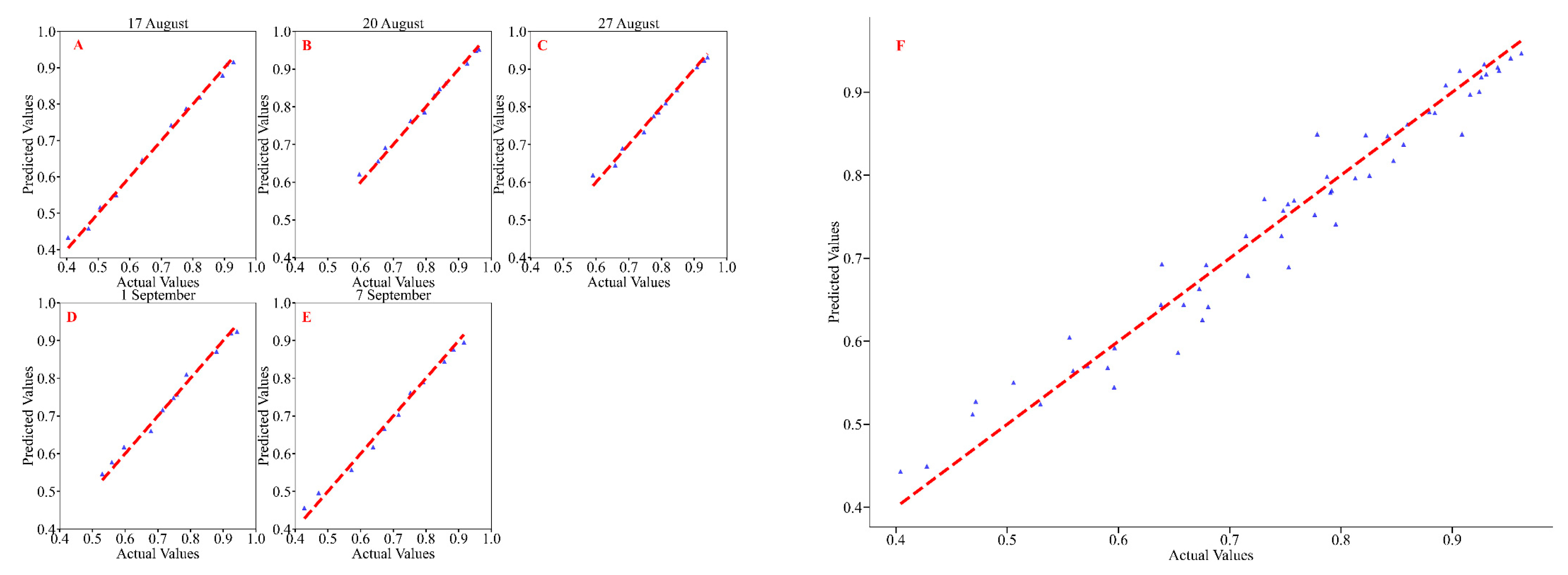
| 17 August (podding stage to beginning of grain stage) | y = −0.00011x2 + 0.02x + 0.313 | 0.981 | 465.967 | <0.001 | 0.011 | 0.001 | 0.013 | 0.995 |
| 20 August (beginning of grain stage to full grain stage) | y = −0.00007x2 + 0.013x + 0.553 | 0.985 | 587.210 | <0.001 | 0.009 | 0.001 | 0.011 | 0.991 |
| 27 August (full grain stage to first maturity stage) | y = −0.00033x2 + 0.027x + 0.403 | 0.987 | 672.916 | <0.001 | 0.009 | 0.001 | 0.012 | 0.989 |
| 1 September (first maturity stage to full grain stage) | y = 0.016x + 0.439 | 0.965 | 249.450 | <0.001 | 0.012 | 0.001 | 0.015 | 0.988 |
| 7 September (full grain stage) | y = −0.00100x2 + 0.044x + 0.205 | 0.972 | 316.937 | <0.001 | 0.015 | 0.001 | 0.016 | 0.989 |
| 17 August to 7 September (podding stage to full grain stage) | y = −0.00025x2 + 0.02403x + 0.38775 | 0.849 | 298.264 | <0.001 | 0.024 | 0.001 | 0.031 | 0.957 |
| Observation Date | Polynomial Regression | Random Forest Regression | ||||||
|---|---|---|---|---|---|---|---|---|
| Fitting Model | R2 | F | p | mae | mse | rmse | R2 | |
| 17 August (podding stage to beginning of grain stage) | y = 145.981x2 − 112.79x + 77.039 | 0.953 | 182.185 | <0.001 | 1.681 | 6.100 | 2.470 | 0.976 |
| 20 August (beginning of grain stage to full grain stage) | y = 315.913x2 − 366.992x + 160.348 | 0.961 | 223.983 | <0.001 | 1.868 | 6.799 | 2.607 | 0.974 |
| 27 August (full grain stage to first maturity stage) | y = 303.712x2 − 330.855x + 142.121 | 0.967 | 260.446 | <0.001 | 1.859 | 6.666 | 2.582 | 0.974 |
| 1 September (first maturity stage to full grain stage) | y = 146.966x2 − 100.863x + 65.566 | 0.964 | 242.715 | <0.001 | 2.019 | 6.962 | 2.638 | 0.973 |
| 7 September (full grain stage) | y = 195.218x2 − 164.304x + 88.513 | 0.983 | 523.781 | <0.001 | 1.602 | 5.708 | 2.389 | 0.978 |
Disclaimer/Publisher’s Note: The statements, opinions and data contained in all publications are solely those of the individual author(s) and contributor(s) and not of MDPI and/or the editor(s). MDPI and/or the editor(s) disclaim responsibility for any injury to people or property resulting from any ideas, methods, instructions or products referred to in the content. |
© 2025 by the authors. Licensee MDPI, Basel, Switzerland. This article is an open access article distributed under the terms and conditions of the Creative Commons Attribution (CC BY) license (https://creativecommons.org/licenses/by/4.0/).
Share and Cite
Meng, W.; Li, X.; Zhang, J.; Pei, T.; Zhang, J. Monitoring of Soybean Bacterial Blight Disease Using Drone-Mounted Multispectral Imaging: A Case Study in Northeast China. Agronomy 2025, 15, 921. https://doi.org/10.3390/agronomy15040921
Meng W, Li X, Zhang J, Pei T, Zhang J. Monitoring of Soybean Bacterial Blight Disease Using Drone-Mounted Multispectral Imaging: A Case Study in Northeast China. Agronomy. 2025; 15(4):921. https://doi.org/10.3390/agronomy15040921
Chicago/Turabian StyleMeng, Weishi, Xiaoshuang Li, Jing Zhang, Tianhao Pei, and Jiahuan Zhang. 2025. "Monitoring of Soybean Bacterial Blight Disease Using Drone-Mounted Multispectral Imaging: A Case Study in Northeast China" Agronomy 15, no. 4: 921. https://doi.org/10.3390/agronomy15040921
APA StyleMeng, W., Li, X., Zhang, J., Pei, T., & Zhang, J. (2025). Monitoring of Soybean Bacterial Blight Disease Using Drone-Mounted Multispectral Imaging: A Case Study in Northeast China. Agronomy, 15(4), 921. https://doi.org/10.3390/agronomy15040921