A Reinforcement Learning-Driven UAV-Based Smart Agriculture System for Extreme Weather Prediction

Abstract

Extreme weather prediction plays a crucial role in agricultural production and disaster prevention. This study proposes a lightweight extreme weather early warning model based on UAV cruise monitoring, a density-aware attention mechanism, and edge computing. Reinforcement learning is utilized to optimize UAV cruise paths, while a Transformer-based model is employed for weather prediction. Experimental results demonstrate that the proposed method achieves an overall prediction accuracy of 0.91, a precision of 0.93, a recall of 0.88, and an F1-score of 0.91. In the prediction of different extreme weather events, the proposed method attains an accuracy of 0.89 for strong wind conditions, 0.92 for hail, and 0.89 for late spring cold, all outperforming state-of-the-art methods. These results validate the effectiveness and applicability of the proposed approach in extreme weather forecasting.

1. Introduction

With the rapid advancement of unmanned aerial vehicle (UAV) technology, its role in the low-altitude economy has become increasingly prominent, particularly in meteorological monitoring, disaster warning, and emergency response [1,2]. Owing to their flexible maneuverability, low-altitude operational capability, and real-time data acquisition features, UAVs have emerged as crucial tools for addressing global climate change and the increasing frequency of extreme weather events [3,4,5]. Compared to traditional ground-based meteorological stations and satellite monitoring, UAVs can penetrate complex terrains and dynamic environments, filling monitoring blind spots and providing high-resolution, multi-dimensional environmental data [6]. However, in practical applications, UAVs still face multiple challenges in path planning, data analysis, and multi-UAV collaboration under complex meteorological conditions [7]. These challenges limit their monitoring efficiency and hinder the integration of low-altitude economic applications with meteorological services. Consequently, exploring efficient and intelligent multi-UAV collaboration techniques can not only significantly enhance monitoring capabilities but also drive innovation in relevant industries [8]. Currently, multi-UAV collaborative monitoring in complex meteorological environments encounters multiple technical bottlenecks. In terms of path planning and task scheduling, traditional methods struggle to achieve efficient task allocation and comprehensive coverage due to uneven sensor data distribution, complex terrain, and communication delays, resulting in high energy consumption and low data acquisition efficiency [9]. Additionally, the limitations of single-source data prevent UAVs from effectively handling the variability and heterogeneity of extreme weather, leading to insufficient data analysis capabilities and inadequate real-time and comprehensive monitoring, thereby affecting early warning accuracy [10]. Moreover, in extreme weather warning tasks at the edge, conventional intelligent models suffer from slow inference speed and processing delays due to the contradiction between computational resource constraints and model complexity, thus failing to meet the high real-time requirements [11,12]. These challenges collectively restrict the potential applications of UAVs in dynamic and complex scenarios, necessitating more adaptive and cooperative solutions.

In recent years, research on UAV path planning and collaborative technologies has made certain advancements. Traditional methods primarily adopt static path planning algorithms, such as Dijkstra’s algorithm or particle swarm optimization, which assign tasks through predefined flight routes in simple environments. However, these approaches exhibit limited adaptability to dynamic meteorological changes, making it difficult to handle sudden obstacles or uneven data distribution [13,14]. With the rise of artificial intelligence and edge computing, machine learning-based approaches have gained increasing attention [15]. For instance, some studies have optimized single-UAV path planning using reinforcement learning to improve obstacle avoidance capabilities. Wang et al. (2024) proposed the APPA-3D algorithm, a reinforcement learning-based 3D path planning method that optimizes reward functions and employs an action selection probability-based exploration strategy, making it suitable for unknown complex environments [16]. Further advancements in deep learning have led to the emergence of novel approaches, such as deep reinforcement learning-based dynamic path-planning algorithms, which can adapt to unknown environments to some extent. For example, Nguyen et al. proposed a UAV trajectory and data collection optimization method based on deep reinforcement learning, designing a reward function that balances data collection and flight paths. By employing grid partitioning, the learning convergence was accelerated, and both deep Q-learning and dueling deep Q-learning algorithms were implemented to achieve near-optimal performance under the constraints of limited flight time and communication [17]. Zhao et al. introduced a UAV-assisted edge computing task offloading method based on multi-agent deep reinforcement learning, jointly optimizing UAV trajectories, task allocation, and communication resource management to minimize total system costs. This approach utilizes the twin delayed deep deterministic policy gradient (TD3) algorithm to handle high-dimensional continuous action spaces, adapting to user mobility and dynamic resource variations [18]. However, the application of these methods under complex meteorological conditions remains constrained by high computational resource demands, insufficient data fusion, and communication delays. Furthermore, most existing research remains at the theoretical level or has small-scale validation, lacking comprehensive solutions tailored for real-world meteorological monitoring scenarios. Therefore, to address these challenges, the development of more efficient and robust technical approaches is imperative.

To overcome these challenges, this study proposes a multi-UAV collaborative monitoring framework for complex meteorological environments, with the following core innovations:

• Enhanced multi-UAV path-planning and coordination efficiency: A reinforcement learning-based dynamic path-planning and coordination algorithm is proposed. By integrating geographical information, real-time UAV communication, and task priority evaluation, the flight paths and collaborative strategies of multiple UAVs are optimized, improving the geographical uniformity and timeliness of data acquisition.
• Multi-source data fusion for improved meteorological monitoring: A multi-source data collaborative fusion mechanism is designed, integrating real-time UAV-acquired data with satellite and ground station data. By leveraging edge–cloud collaborative computing, data complementarity and comprehensiveness are enhanced, thereby improving monitoring accuracy and support capabilities under complex meteorological conditions.
• Lightweight intelligent early warning model for real-time extreme weather detection: A lightweight intelligent early warning model is introduced. Through model pruning and parameter optimization, its deployment on UAVs is achieved, while edge inference acceleration techniques significantly enhance real-time data processing capabilities, ensuring the timeliness and accuracy of extreme weather warnings.
• The effectiveness of the proposed framework has been validated through experiments and field tests. Results demonstrate that the proposed method significantly outperforms traditional approaches in terms of data acquisition efficiency, monitoring accuracy, and early warning timeliness. This study provides a feasible solution for intelligent multi-UAV monitoring under complex meteorological conditions and lays a technological foundation for the further development of the low-altitude economy.

2. Materials and Methods

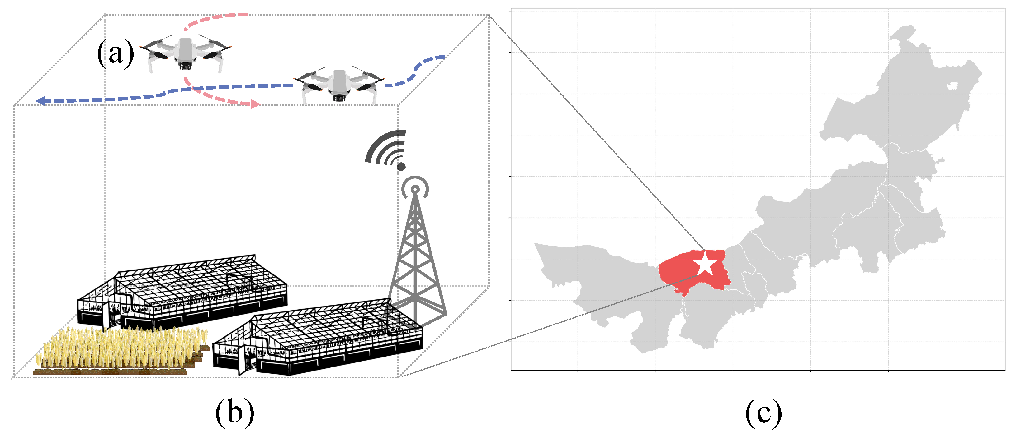
2.1. Materials Acquisition

As shown in Figure 1, the data collection for this study was conducted in the meteorological station of Wuyuan County, Bayannur City, Inner Mongolia, and the surrounding farmland areas and was designed to establish an edge-intelligent extreme weather early warning system based on UAVs. A combination of fixed-wing and rotary-wing UAVs was utilized to ensure comprehensive and accurate data acquisition. Specifically, the fixed-wing UAV (eBee X, SenseFly, Lausanne, Switzerland) was employed for large-scale surveillance due to its extended endurance, enabling it to cover extensive farmland and meteorological monitoring areas. In contrast, the rotary-wing UAV (Matrice 300 RTK (DJI, Shenzhen, China)) was utilized for high-precision monitoring, equipped with multiple sensors to flexibly adjust flight altitude for enhanced data accuracy. The data collection was carried out from January 2024 to December 2024, encompassing all four seasons to ensure the completeness of extreme weather data. The UAVs executed flight missions according to predefined flight paths. The fixed-wing UAV primarily conducted high-altitude patrols along the boundaries of farmland and near meteorological stations, operating at an altitude of approximately 120 m, a cruising speed of 12 m/s, and a flight radius of about 10 km. The rotary-wing UAV dynamically adjusted its flight parameters based on weather conditions and areas requiring focused monitoring, maintaining an altitude of 30–80 m and a speed of 3–5 m/s, with particular emphasis on high-precision data acquisition in anomalous meteorological regions.

The collected data consisted of two major categories: environmental meteorological data and optical imaging data. The environmental meteorological data, including temperature, humidity, pressure, wind speed, wind direction, and precipitation, were primarily collected using the ATMOS-41 meteorological sensor (METER Group) (METER Group) mounted on the fixed-wing UAV.

As shown in

Table 1. Meteorological and images collected in this study.

Parameter	Abbreviation	Measurement Unit
Temperature	Tair	°C
Humidity	Hum	%
Pressure	Pres	hPa
Wind speed	WS	m s−1
Wind direction	WD	°
Precipitation	Prec	mm
Visible light image	Vis	-
Infrared thermal image	IR	-

, this sensor simultaneously measured key atmospheric indicators, including air temperature ranging from −40 °C to 60 °C with an accuracy of ±0.3 °C, relative humidity from 0% to 100% with an accuracy of ±2%, atmospheric pressure from 300 to 1200 hPa with an accuracy of ±0.4 hPa, and wind speed from 0 to 60 m/s with an accuracy of ±0.3 m/s. Additionally, supplementary data were provided by the Wuyuan County Meteorological Station to calibrate and validate the UAV-acquired measurements. The optical and imaging data were obtained using multi-spectral and infrared sensors mounted on the rotary-wing UAV. The visible light images were captured using the Zenmuse H20T sensor (DJI, Shenzhen, China), providing a resolution of 20 MP for monitoring visibility and precipitation morphology. Infrared thermal imaging data were acquired using the FLIR Vue Pro R 640 (FLIR Systems), covering a temperature measurement range from −40 °C to +150 °C with an accuracy of ±0.05 °C, enabling the assessment of surface temperature variations and the prediction of frost and heat stress. To ensure data stability and accuracy, orthomosaic stitching and multi-spectral fusion techniques were employed to eliminate stitching errors and enhance spectral information representation.

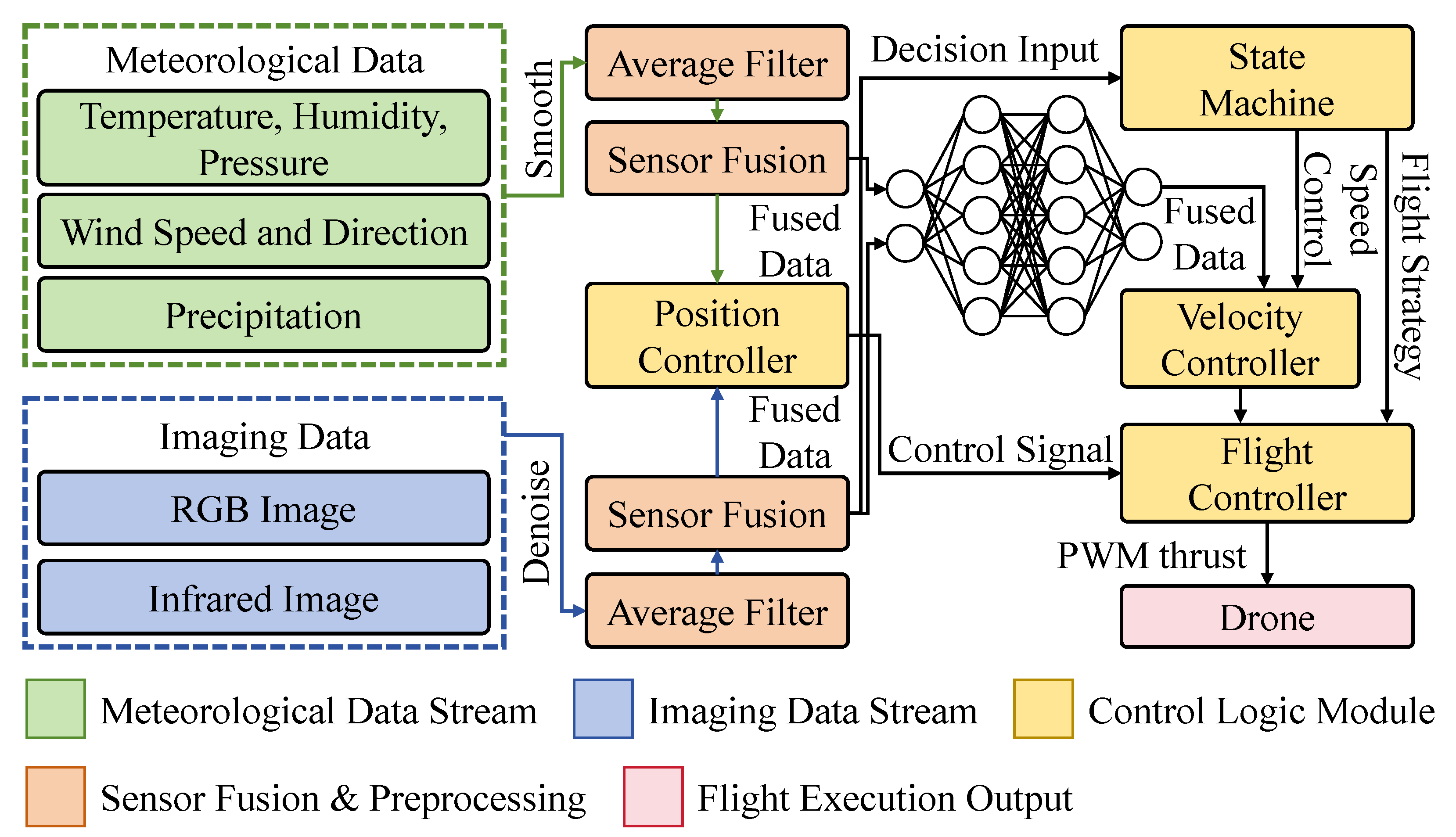
2.2. Data Preprocessing

2.2.1. Sensor Data Preprocessing

In the initial stage of data processing, all sensor data were synchronized to ensure the alignment of timestamps across different data sources. The meteorological sensor ATMOS-41 mounted on the UAV was compared with ground meteorological station data. A moving average filter was applied to smooth transient fluctuations in short time intervals, while dynamic time warping was utilized to correct the temporal sequence of data, minimizing time shifts between different sensors. For anomaly detection, the three-sigma ($3\sigma$) rule was employed to eliminate outliers, and historical meteorological data were used to set reasonable threshold ranges to exclude physically unrealistic measurements. In winter in Bayannur, temperatures typically do not exceed 40 °C; therefore, any recorded values beyond this range were filtered out. Additionally, locally weighted regression was applied for missing data interpolation to ensure the completeness of the time-series data. Fourier transform was used to analyze the periodic components of wind speed and wind direction data, allowing the identification and removal of transiently disturbed measurements. For precipitation data, sensor false alarms or measurement errors were mitigated by referencing ground-based rain gauge data, and a Kalman filter was applied to estimate sensor data states, enhancing measurement stability and accuracy. Following preprocessing, spatial calibration of meteorological data was conducted to ensure geographic consistency. During UAV flights, meteorological sensors might experience airflow disturbances, leading to fluctuations in recorded values. Thus, real-time kinematic GPS data were incorporated for positional calibration. Interpolation techniques were used to align measurements from different altitudes and flight paths with ground station data, thereby improving the spatial distribution accuracy. Furthermore, to reduce data noise and enhance the generalization capability of the predictive model, principal component analysis was employed to perform dimensionality reduction on high-dimensional meteorological data, extracting key feature variables while reducing computational complexity without compromising critical information.

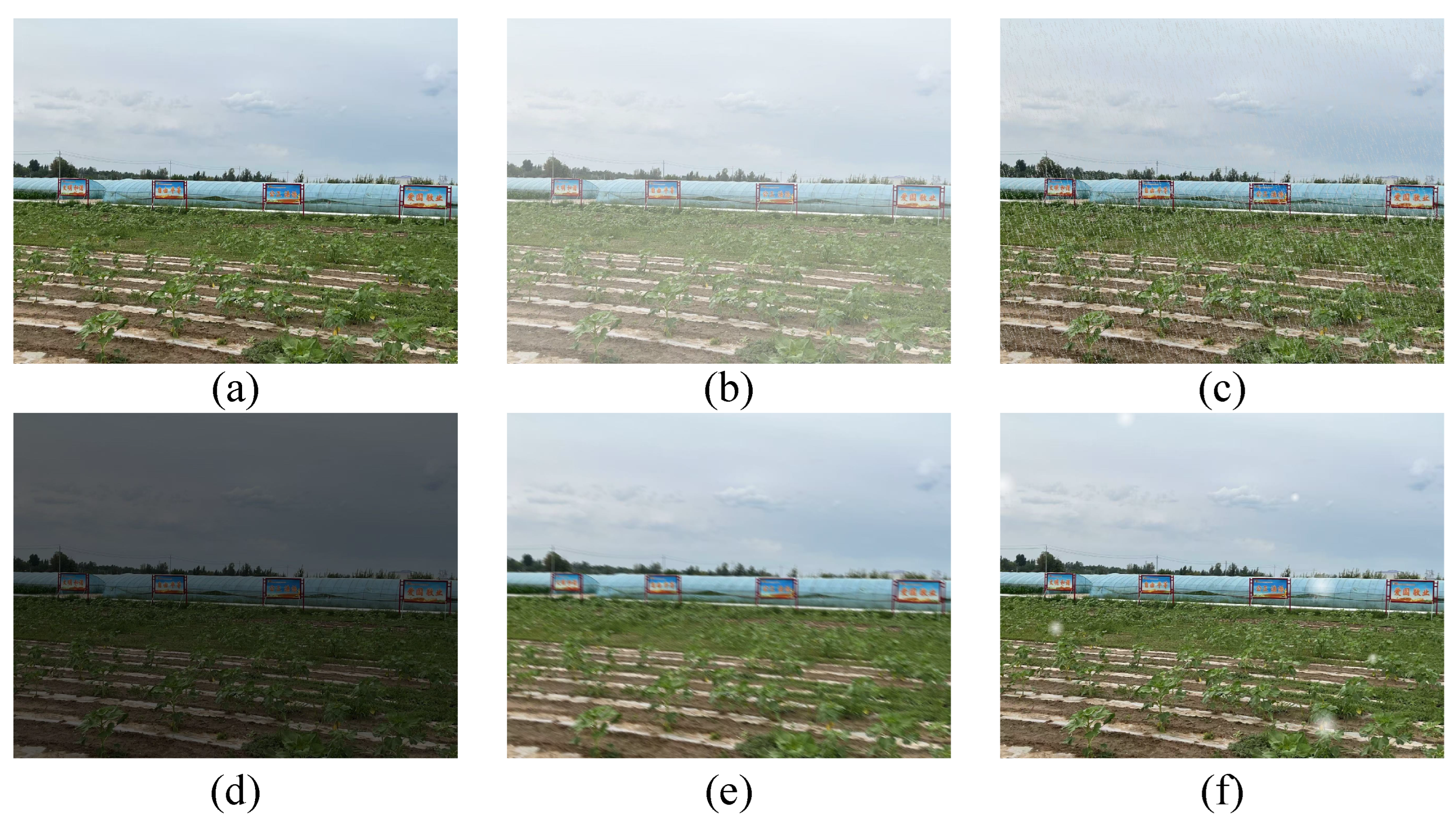
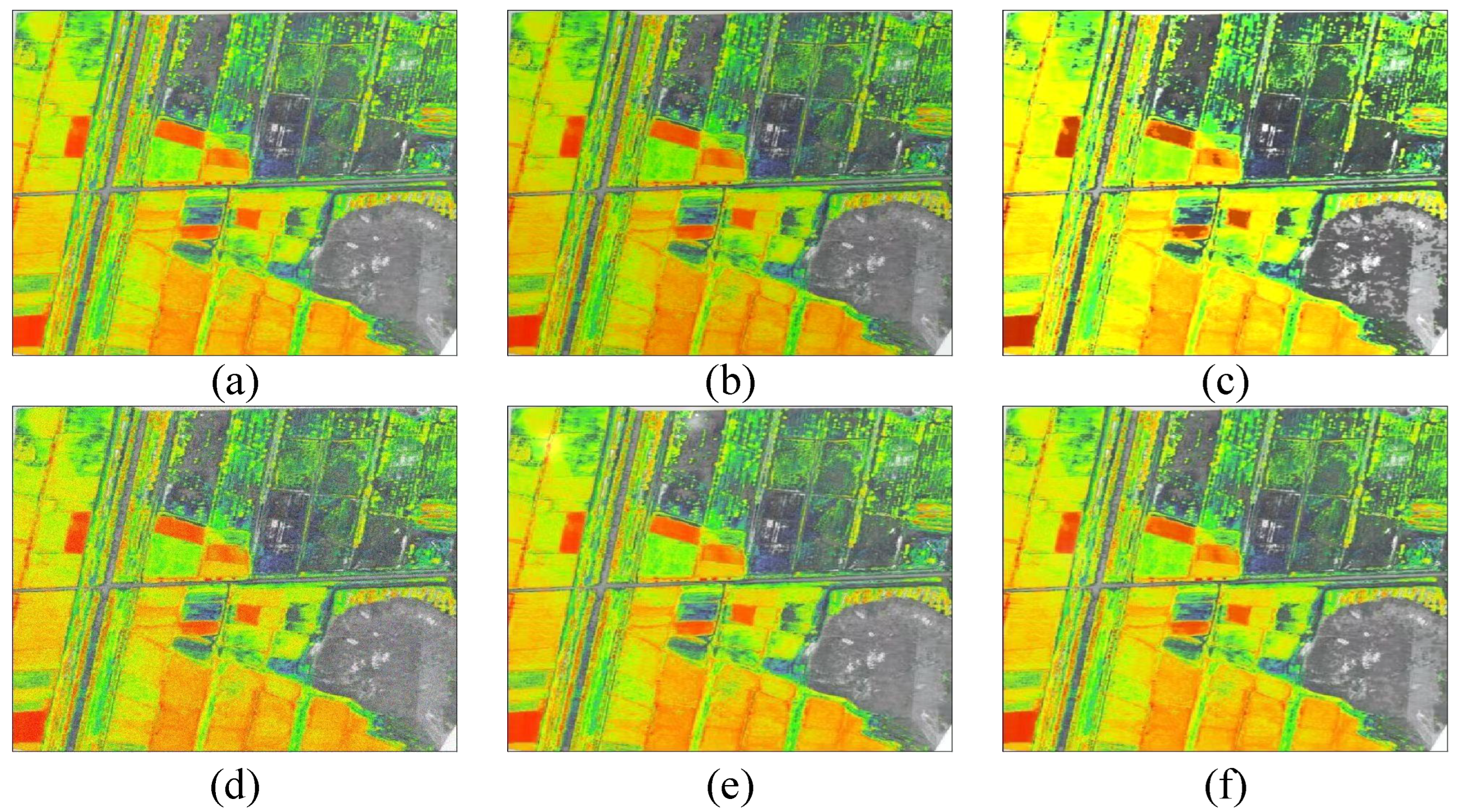
2.2.2. Image Data Preprocessing

During the data augmentation process, various image enhancement techniques tailored to visible light and infrared thermal imaging were designed and applied for the collaborative monitoring tasks of multiple unmanned aerial vehicles (UAVs) in complex meteorological environments.

The robustness and adaptability of the monitoring model were improved, ensuring stable performance under diverse conditions such as fog, rain, low illumination, and extreme temperatures, as illustrated in Figure 2. For visible light data, augmentation methods including fog enhancement, rainfall synthesis, low-light enhancement, dynamic blur, and reflective light interference were employed. Fog enhancement was implemented by simulating fog environments of varying densities, enabling the model to adapt to reduced visibility scenarios and learn to extract key features under foggy conditions. Rainfall synthesis was achieved by generating randomly distributed raindrops and streaks, simulating the interference of rainy weather on images and enhancing the model’s robustness to rain-affected data. Low-light enhancement was conducted by reducing image brightness and introducing characteristics of insufficient illumination, training the model to accurately identify targets in nighttime or low-light settings. Dynamic blur was utilized to simulate image jitter caused by high-speed UAV flight or strong wind interference, improving the model’s adaptability to motion blur. Reflective light interference was introduced by adding random light spots or highlighted areas to the images, simulating natural phenomena such as sunlight reflection or water surface glare, ensuring that recognition accuracy is maintained under strong light disturbances.

As shown in Figure 3, for infrared thermal imaging data, augmentation strategies such as temperature drift simulation, high- and low-temperature region expansion, thermal texture noise, localized heat source simulation, and multispectral fusion were introduced. Temperature drift simulation was performed by randomly adjusting the overall temperature distribution of infrared images, mimicking the interference of ambient temperature changes on thermal imaging and enhancing the model’s adaptability to temperature fluctuations. High- and low-temperature region expansion was executed by amplifying or attenuating the contrast of hot and cold regions in the images, broadening the model’s perception capability under extreme temperature conditions. Thermal texture noise was added by superimposing random thermal noise patterns, simulating signal distortions from imaging equipment or transmission processes and strengthening the model’s robustness to low-quality thermal imaging data. Localized heat source simulation was implemented by randomly inserting small-scale heat source regions into the images, training the model to distinguish target features in complex thermal distribution scenarios. Multispectral fusion was achieved by combining visible light and infrared thermal imaging data to generate composite images, encouraging the model to learn the complementarity of multimodal features and thereby enhancing comprehensive monitoring capabilities under complex meteorological conditions.

2.3. Proposed Method

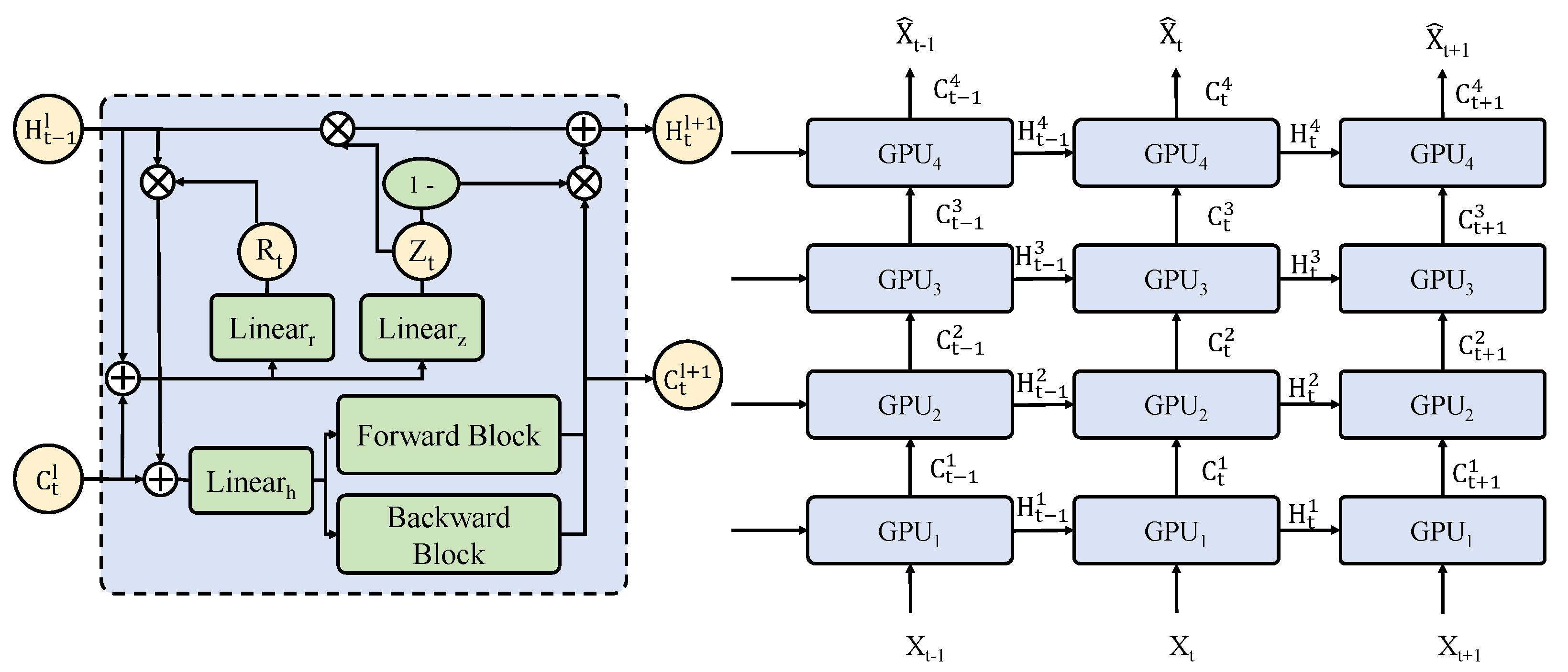
2.3.1. Overall

As shown in Figure 4, the proposed methodology consists of multiple modules, beginning with data input, where processed meteorological data, including temperature, humidity, pressure, wind speed, wind direction, and precipitation, along with imaging data, such as visible light and infrared thermal images, are fed into separate submodules. The meteorological data are processed by the edge-computing-based, lightweight, extreme weather early warning model, while the imaging data undergo feature extraction and regional optimization via the density-aware attention mechanism. During UAV mission planning, a reinforcement learning-driven path optimization algorithm is employed, aiming to maximize information gain. The UAV state is defined as

$$S_t=\{x_t,y_t,v_t,T_t,H_t,P_t,W_t,D_t\},$$

(1)

where $x_t$ and $y_t$ represent the spatial coordinates, $v_t$ is the velocity, and $T_t$, $H_t$, $P_t$, $W_t$, and $D_t$ denote the air temperature (°C), relative humidity (%), atmospheric pressure (hPa), wind speed (m/s), and wind direction (°), respectively. The optimal flight path is dynamically adjusted based on the reward function

$$R_t=w_1·I{G}_t-w_2·E_t-w_3·C_t,$$

(2)

where $I{G}_t$ represents information gain, $E_t$ denotes energy consumption, and $C_t$ accounts for collision avoidance constraints, $w_1$, $w_2$, and $w_3$ represent the weights of information gain, energy consumption penalty, and collision avoidance cost, respectively. The density-aware attention mechanism is designed to enhance the detection accuracy in high-density extreme weather regions by applying weighted optimization. The attention weight is computed using kernel density estimation as follows:

$$D(x,y)=\sum _{i=1}^{N}K\left({\displaystyle \frac{{(x-x_i)}^2+{(y-y_i)}^2}{h^2}}\right),$$

(3)

where $K(·)$ is the kernel function and h is the bandwidth parameter. This approach ensures improved sensitivity to extreme weather anomalies. Finally, the optimized data are processed using the Transformer-based WeatherNet model, which employs a hierarchical self-attention mechanism to extract spatiotemporal features. The model is further optimized with L1 pruning and 8-bit post-training quantization to enable efficient inference on edge devices. After initial inference at the UAV edge node, results are transmitted via 5G or LoRa to the cloud, where global data fusion analysis is performed to enhance the accuracy of extreme weather warnings.

2.3.2. UAV Cruise Optimization Algorithm

As shown in Figure 5, a reinforcement learning-based UAV cruise optimization algorithm was designed in this study, incorporating a deep neural network structure to enhance UAV adaptability under complex meteorological conditions and improve data acquisition efficiency. To enhance the robustness and stability of the UAV flight policy, the proximal policy optimization algorithm was used, with convergence assessed through the average cumulative reward and policy loss. The reward weights $w_1$, $w_2$, and $w_3$ were tuned via grid search and finalized as $w_1=1.0$, $w_2=0.6$, and $w_3=0.4$. The training environment was constructed using Unity, integrating terrain data and dynamic meteorological conditions to support interactive, high-fidelity simulations. The proximal policy optimization convergence was achieved after approximately 1500 iterations, with the policy exhibiting strong generalization performance.

The model consists of a three-layer network structure, including an input layer, hidden layers, and an output layer, where parameters are optimized to accommodate high-dimensional UAV state inputs and continuous control outputs. The input layer incorporates environmental variables and UAV state data with dimensions $(W,H,C)=(10,10,6)$, where the $10\times 10$ grid represents meteorological regions and the six channels correspond to temperature, humidity, pressure, wind speed, wind direction, and precipitation. The hidden layers consist of two fully connected layers and one convolutional layer. The first fully connected layer contains 128 neurons with a ReLU activation function to enhance nonlinearity. The convolutional layer employs a $3\times 3$ kernel with 64 channels to extract local meteorological patterns. The second fully connected layer is designed with 64 neurons and uses a Sigmoid activation function to ensure output stability. The output layer maps the UAV’s flight action space, including adjustments in heading angle $\mathrm{\Delta }\theta$, flight speed $\mathrm{\Delta }v$, and flight altitude $\mathrm{\Delta }h$. The objective of the cruise optimization algorithm is to minimize UAV energy consumption E while maximizing the coverage of extreme weather regions. The reinforcement learning policy ${\pi }_{\theta }\left(a_t\right|s_t)$ is optimized using a policy gradient approach, with the loss function defined as

$$J\left(\theta \right)=\mathbb{E}\left[\sum _{t=0}^T{\gamma }^t{R}_t\right],$$

(4)

where $R_t$ is the reward function at time step t and $\gamma$ is the discount factor, set to 0.99 to ensure long-term optimization. The reward function integrates information gain $I{G}_t$, UAV energy consumption $E_t$, and obstacle avoidance cost $C_t$, where $I{G}_t$ is derived from meteorological information entropy using Shannon entropy:

$$I{G}_t=-\sum _{i}P\left(x_i\right)logP\left(x_i\right).$$

(5)

UAV energy consumption is computed based on flight speed and aerodynamic drag using the following equation:

$$E_t={\displaystyle \frac{1}{2}}{C}_d\rho A{v}^3,$$

(6)

where $C_d$ is the drag coefficient, $\rho$ represents air density, A denotes the UAV’s frontal area, and v is the flight velocity. The obstacle avoidance cost $C_t$ is determined based on the minimum safe distance $d_{\mathrm{safe}}$ and the actual obstacle distance $d_{\mathrm{obs}}$:

$$C_t=max(0,d_{\mathrm{safe}}-d_{\mathrm{obs}}).$$

(7)

The proximal policy optimization algorithm was used to train the proposed reinforcement learning model. A clipped surrogate objective function was adopted to stabilize learning and limit policy updates:

$$L\left(\theta \right)={\mathbb{E}}_t\left[min(r_t\left(\theta \right)A_t,\mathrm{clip}(r_t\left(\theta \right),1-ϵ,1+ϵ)A_t)\right],$$

(8)

where $r_t\left(\theta \right)$ represents the policy ratio and $ϵ$ is set to 0.2 to constrain policy updates. The proposed algorithm provides several advantages in UAV mission planning. First, reinforcement learning-based cruise optimization enables dynamic adaptation to meteorological variations, improving data acquisition efficiency. Second, the integration of a density-aware attention mechanism enhances the focus on high-risk weather regions, thereby improving extreme weather prediction accuracy. Additionally, combining edge computing with low-power AI inference allows UAVs to autonomously adjust flight paths over extended durations, enhancing monitoring coverage and reliability.

2.3.3. Density-Aware Attention Mechanism

As shown in Figure 6, the density-aware attention module is designed to enhance the sensitivity of extreme weather monitoring compared to traditional self-attention. While SA primarily computes global correlations within an input sequence through query, key, and value matrices, a density-aware attention module incorporates spatial density estimation to adapt the model’s focus based on the spatial distribution characteristics of meteorological variables. In the proposed density-aware attention module, density estimation is first applied to the input meteorological tensor X, which has dimensions $(W,H,C)=(64,64,6)$. Here, $64\times 64$ represents the spatial dimensions and $C=6$ corresponds to six meteorological channels: temperature, humidity, pressure, wind speed, wind direction, and precipitation. Kernel density estimation is employed to compute the density distribution of each spatial point. The computed density $D(x,y)$ is then normalized and incorporated into the attention mechanism by adjusting the query weight:

$$Q^{\prime }=D\odot Q,$$

(9)

where Q represents the original query matrix in standard self-attention and ⊙ denotes element-wise multiplication. The modified attention scores are computed as follows:

$$A=\mathrm{softmax}\left({\displaystyle \frac{Q^{\prime }{K}^T}{\sqrt{d_k}}}\right).$$

(10)

Finally, the attention output is computed using the standard formulation: $Z=AV$. The proposed density-aware attention module is integrated into a four-layer Transformer architecture, where each layer contains a density-aware attention module. The input features are first processed through a $3\times 3$ convolutional layer with 64 channels before being fed into the Transformer. Each Transformer layer processes inputs of dimensions $(64,64,64)$, maintaining the same output size. The computational complexity of the density estimation module is $O\left(N^2\right)$. However, by employing spatial pyramid pooling for feature downsampling, the final computational complexity is reduced to $O(NlogN)$. Compared to traditional self-attention mechanisms, the density-aware attention module enhances the model’s ability to focus on extreme weather regions, thereby improving detection accuracy. Additionally, the incorporation of a local weighting mechanism within the attention computation reduces computational resource consumption in low-density regions, increasing inference efficiency. This optimization ensures that UAVs can perform real-time extreme weather monitoring efficiently within an edge computing environment.

2.3.4. Lightweight Edge-Computing-Based Extreme Weather Early Warning Model

The proposed lightweight extreme weather early warning model based on edge computing employs Transformer-based WeatherNet as the core predictive framework. To optimize computational efficiency and accommodate UAV resource constraints while maintaining accuracy and real-time processing capability, model pruning, quantization, and knowledge distillation techniques are incorporated. The overall model architecture consists of an input feature extraction layer, a density-aware attention module, a spatiotemporal feature fusion module, and a final weather prediction module. The input data are collected from UAV meteorological observations, including temperature, humidity, pressure, wind speed, wind direction, and precipitation as well as optical and infrared imaging data. The input dimensions are $(W,H,C)=(64,64,6)$, where $W=H=64$ represents the spatial resolution and $C=6$ corresponds to the six meteorological variables. The feature extraction layer first applies a $3\times 3$ convolutional layer with 64 channels, utilizing the Swish activation function to ensure a smooth feature distribution, thereby stabilizing subsequent Transformer training. The extracted features are then processed by the density-aware attention module, which extends traditional self-attention by incorporating density-weighted adjustments to enhance sensitivity to high-density meteorological anomaly regions. Finally, the attention output is obtained using $Z=AV$. After processing by the density-aware attention module, the output features are passed into the spatiotemporal feature fusion module, which employs a dual-branch architecture. One branch utilizes a Bi-LSTM network to capture temporal dependencies, while the other employs a ResNet for spatial feature extraction. Given an input sequence $X_t$, the temporal features are computed by the Bi-LSTM network as follows:

$$h_t=\sigma (W_h{h}_{t-1}+W_x{X}_t+b_h).$$

(11)

Simultaneously, the spatial features are extracted using ResNet:

$$F=X+\mathrm{Conv}\left(\mathrm{ReLU}\right(\mathrm{Conv}\left(X\right)\left)\right).$$

(12)

The outputs of the two branches are fused using

$$Y=W_T{h}_t+W_{F}F.$$

(13)

The final weather prediction module utilizes Transformer-based WeatherNet, which consists of four Transformer layers, each containing 64 attention heads and a hidden dimension of 256. The GELU activation function is applied, and LayerNorm is used for normalization. To further optimize computational efficiency, model pruning and quantization techniques are employed. L1-based pruning removes weights below a predefined threshold $\lambda$:

$$W^{\prime }=W·\mathbb{I}\left(\right|W|>\lambda ).$$

(14)

For quantization, an 8-bit post-training quantization is applied, converting floating-point values into fixed-point representations:

$$Q\left(W\right)=\mathrm{round}\left({\displaystyle \frac{W-W_{min}}{W_{max}-W_{min}}}\times 255\right).$$

(15)

The final inference results are transmitted to the cloud for fusion analysis. Given the limited computational resources on UAVs, edge computing significantly reduces the computational burden, enabling real-time early warning tasks to be executed efficiently in low-power environments while maintaining high prediction accuracy. By integrating model pruning and quantization, the inference complexity at the UAV edge device is reduced from $O\left(N^2\right)$ to $O(NlogN)$, enabling millisecond-level inference under a 10 W power constraint, which meets the operational requirements for long-duration UAV missions.

2.4. Experimental Setup

2.4.1. Hardware and Software Platform

The experimental environment in this study comprises UAV computing units, sensor equipment, and a server computing platform to ensure stable data acquisition and efficient model training. All UAVs are equipped with a real-time kinematic system, integrated with a global navigation satellite system for high-precision positioning, achieving a horizontal accuracy of up to 1 cm to maintain spatiotemporal consistency in the collected data. The UAV computing unit is powered by an NVIDIA Jetson Xavier NX (NVIDIA Corporation, Santa Clara, CA, USA), featuring a 384-core CUDA GPU and a 6-core ARM CPU, with support for TensorRT-accelerated inference, enabling efficient execution of edge computing tasks. On the server side, an NVIDIA A100 GPU is utilized for deep learning model training and optimization, equipped with 80 GB of HBM2 memory and supporting FP16 computation to enhance the training efficiency of Transformer-based architectures. Data storage and management are implemented using a distributed file system, integrating Hadoop HDFS with the Spark computing framework to facilitate large-scale meteorological data processing through parallel computation and real-time streaming analytics.

2.4.2. Experimental Configuration

The dataset was partitioned into training, validation, and test sets in a 7:2:1 ratio. Specifically, 70% of the data was allocated to the training set for optimizing model parameters and learning multi-source data features, including both drone-based and ground-based data. The validation set accounted for 20% of the data and was primarily used for hyperparameter tuning and monitoring overfitting during the training process. The remaining 10% was assigned to the test set to evaluate the model’s final performance in weather prediction tasks. This partitioning strategy was chosen to ensure that the model effectively leverages the collected diverse data while preserving independent subsets for validating its predictive capabilities. To further enhance the model’s robustness and generalization ability, a 10-fold cross-validation approach was employed. In this method, the dataset was divided into ten equal subsets, with nine subsets used for training and the remaining one subset designated as the validation set in each iteration. This process was repeated 10 times, ensuring that each sample was used for validation at least once, thereby reducing the impact of random data partitioning on model performance. A stratified sampling method was applied during the partitioning process to maintain balanced data distribution across the training, validation, and test sets. Given the diversity of weather patterns (e.g., sunny, rainy, extreme weather), special attention was given to class balance to ensure that each subset accurately reflected the overall data distribution. To mitigate potential biases introduced by random partitioning, multiple rounds of random resampling were conducted after the initial split. The training results under different partitioning strategies were compared to verify the stability of model performance. This approach ensured that the weather prediction model, which integrates sensor data from both drones and ground-based sources, remained unaffected by inconsistencies in data partitioning.

2.4.3. Evaluation Metrics

A comprehensive evaluation of the model’s performance in weather prediction tasks was conducted using a set of commonly employed evaluation metrics. These include precision (P), recall (R), accuracy ($Acc$), and F1-score ($F1$) for classification tasks, as well as mean absolute error (MAE), root mean square error (RMSE), and the coefficient of determination ($R^2$) for regression tasks. These metrics assess the model’s effectiveness from both classification and regression perspectives, ensuring the accurate prediction of weather categories (e.g., sunny, rainy) while maintaining high precision in forecasting continuous variables such as temperature and precipitation.

$$P={\displaystyle \frac{TP}{TP+FP}}$$

(16)

$$R={\displaystyle \frac{TP}{TP+FN}}$$

(17)

$$Acc={\displaystyle \frac{TP+TN}{TP+TN+FP+FN}}$$

(18)

$$F1=2\times {\displaystyle \frac{P\times R}{P+R}}$$

(19)

$$MAE={\displaystyle \frac{1}{N}}\sum _{i=1}^N|y_i-\widehat{y}i|$$

(20)

$$RMSE=\sqrt{{\displaystyle \frac{1}{N}}\sum {i=1}^N{(y_i-\widehat{y}i)}^2}$$

(21)

$$R^2=1-{\displaystyle \frac{\sum {i=1}^N{(y_i-\widehat{y}i)}^2}{\sum {i=1}^N{(y_i-\overline{y})}^2}}$$

(22)

In these equations, $TP$ (true positives) denotes the number of correctly predicted weather categories, while $FP$ (false positives) represents the number of samples incorrectly classified as a specific weather type. Similarly, $FN$ (false negatives) indicates the number of actual weather categories that were not correctly predicted, and $TN$ (true negatives) refers to samples correctly classified as non-target weather categories. For regression tasks, $y_i$ represents the actual value, ${\widehat{y}}_i$ denotes the predicted value, $\overline{y}$ is the mean of the actual values, and N is the total number of samples. The classification metrics (P, R, $Acc$, and $F1$) are employed to evaluate the model’s capability in weather classification tasks, ensuring effective differentiation between weather patterns while minimizing false alarms and missed detections. The regression metrics ($MAE$, $RMSE$, and $R^2$) measure the model’s accuracy and explanatory power in continuous weather parameter forecasting, ensuring minimal deviation between predicted and observed values while reflecting the model’s ability to fit data variations.

2.5. Baseline

ARIMA [19] is recognized as a classic time series forecasting model, integrating autoregressive, differencing, and moving average components to capture linear relationships and seasonal patterns. Its application is widely observed in financial and economic forecasting. LSTM [20] is characterized as a specialized recurrent neural network, addressing the vanishing gradient problem through gating mechanisms. It excels in learning long-term dependencies and is deemed suitable for sequence modeling, speech recognition, and natural language processing. ConvLSTM [21] is regarded as an extension of LSTM, incorporating convolutional operations to simultaneously capture spatiotemporal dependencies. Its utility is demonstrated in tasks such as video sequence prediction and meteorological forecasting. MetNet [22] is identified as a neural weather model specifically designed for high-precision precipitation forecasting. It leverages deep networks to learn from radar and satellite data, predicting precipitation over future time periods. An axial self-attention mechanism is employed to aggregate extensive spatial information, offering rapid computation and outperforming traditional numerical weather prediction over extended forecast horizons. DWFH [23] is described as a data-driven deep weather forecasting hybrid model, utilizing a transductive long short-term memory network to process meteorological time series. Prediction optimization is achieved through test data similarity, with superior performance noted in forecasting parameters such as temperature and humidity. TMC-Net [24] is presented as a multivariate time series fusion temperature forecast correction network. Temporal feature extraction, multi-scale fusion, and Transformer modules are integrated to mitigate numerical forecast errors, enhancing accuracy through historical information and attention mechanisms. STTN [25] is introduced as a Transformer-based spatiotemporal forecasting model. Global and local positional encodings are utilized to capture multi-scale spatial information, while a temporal Transformer extracts long-range dependencies. Its applicability to weather forecasting is supported by extensive experiments on real-world weather datasets, confirming the framework’s effectiveness.

3. Results and Discussion

3.1. Overall Performance of Different Models in Extreme Weather Prediction

The objective of this experiment was to evaluate the performance of different models in extreme weather prediction, focusing on four key metrics: precision, recall, accuracy, and F1-score. Several baseline models were employed, including the traditional time-series model ARIMA, deep learning models such as LSTM, and hybrid models integrating convolutional and recurrent networks, such as ConvLSTM. Additionally, several recently proposed weather forecasting models, including METNet, DWFH, TMC-Net, and STTN, were assessed. The experimental data were obtained from UAV meteorological observations, processed using DAAM, and subsequently input into different models for prediction. Performance was measured based on the four evaluation metrics.

As shown in

Table 2. Experimental results of the proposed models.

Model	Precision	Recall	Accuracy	F1-Score
ARIMA [19]	0.81	0.84	0.82	0.82
LSTM [20]	0.83	0.85	0.83	0.84
METNet [22]	0.85	0.86	0.84	0.85
DWFH [23]	0.85	0.87	0.86	0.86
ConvLSTM [21]	0.86	0.89	0.87	0.87
TMC-Net [24]	0.88	0.85	0.87	0.86
STTN [25]	0.91	0.89	0.90	0.90
Proposed Method	0.93	0.88	0.91	0.91

and Figure 7, the experimental results indicate that the traditional statistical model ARIMA exhibits relatively lower performance across all metrics. In contrast, LSTM and ConvLSTM demonstrate improvements in accuracy and F1-score due to their capability to model long-term dependencies. METNet and DWFH, which integrate convolutional and recurrent neural networks, further enhance spatiotemporal feature extraction, resulting in slightly higher prediction accuracy compared to standalone LSTM architectures. TMC-Net, by incorporating a multivariate correction mechanism, achieves a precision of 0.88 but exhibits a lower recall of 0.85, suggesting a higher miss rate for certain extreme weather events. The STTN model, which leverages a spatiotemporal Transformer framework, effectively captures long-term dependencies in time-series data while integrating spatial features, leading to consistently high performance across all four evaluation metrics, with scores exceeding 0.89. The proposed method outperforms all baseline models across all metrics, achieving a precision of 0.93 and an F1-score of 0.91, demonstrating superior robustness and generalization capability in extreme weather prediction tasks. The mathematical characteristics of different models influence their performance in this task. ARIMA, as a traditional time-series model, is based on the combination of autoregressive and moving average components. However, its reliance on linear modeling limits its adaptability to complex nonlinear extreme weather patterns, resulting in inferior performance compared to deep learning models. LSTM, with its gated mechanism (input gate, forget gate, and output gate), effectively mitigates long-term dependency issues and surpasses ARIMA in performance. Nevertheless, due to its lack of explicit spatial modeling capabilities, its accuracy remains lower than that of ConvLSTM and Transformer-based models. ConvLSTM, by incorporating convolutional operations into the LSTM structure, enables the state transition matrix to capture local spatial patterns. This enhancement leads to a higher recall of 0.89 in the experiment, indicating improved sensitivity in detecting extreme weather events. STTN and the proposed method are based on Transformer architectures. The proposed method further integrates the density-aware attention mechanism, which adjusts attention distribution based on the spatial density of meteorological variables. This modification enhances the model’s ability to focus on high-density extreme weather regions, leading to improved precision and F1-score. Consequently, the proposed approach achieves the best overall performance among all tested models, demonstrating its effectiveness in extreme weather forecasting.

3.2. Performance of Different Models in Various Extreme Weather Conditions

The objective of this experiment was to evaluate the predictive capabilities of different models under three extreme weather conditions: hail, strong wind, and late spring cold. Due to the varying temporal scales, spatial distribution characteristics, and formation mechanisms of these extreme weather events, a single model may perform well in specific weather types but exhibit limitations in others. To assess these differences, multiple time-series and deep learning models were evaluated, including the traditional statistical model ARIMA, recurrent neural networks such as LSTM, hybrid CNN–RNN models like METNet, DWFH, and ConvLSTM, as well as state-of-the-art Transformer-based architectures, including STTN and TMC-Net.

As shown in Figure 8, the experimental results indicate that different models exhibit varying performances in predicting different types of extreme weather events. As a traditional time series model, ARIMA demonstrates relatively low prediction accuracy across all extreme weather categories, ranging from 0.81 to 0.82, suggesting its limited adaptability to highly nonlinear and non-stationary extreme weather data. LSTM, benefiting from its capability to capture long-term and short-term dependencies in time series modeling, achieves prediction accuracies of 0.83 and 0.81 for hail and strong wind events, respectively, which are slightly superior to those of ARIMA. However, its accuracy for late spring cold spell prediction is only 0.80, indicating certain limitations when handling highly abrupt weather phenomena. In contrast, METNet, which integrates CNNs for spatial feature extraction, improves prediction accuracy for late spring cold spells at 0.85, surpassing LSTM, while its performance for hail and strong wind events (0.83 and 0.82) remains comparable to that of LSTM. DWFH enhances modeling capabilities for complex weather events through multi-scale feature extraction, achieving prediction accuracies of 0.85, 0.87, and 0.84 for hail, strong wind, and late spring cold spells, respectively, showing improvements over the aforementioned models. ConvLSTM incorporates convolutional operations into the LSTM structure to enhance local spatial feature modeling, resulting in increased prediction accuracies of 0.89 and 0.87 for hail and strong wind events, respectively, further strengthening its weather forecasting capability. TMC-Net, which integrates time series modeling with a multivariable correction mechanism, performs well in predicting strong wind and late spring cold spells, achieving accuracies of 0.88 and 0.86, respectively. However, its performance for hail prediction is slightly inferior to ConvLSTM, reaching only 0.87. As a spatiotemporal modeling approach based on Transformer architecture, STTN improves long-sequence modeling capability through a global attention mechanism, achieving the highest accuracy for hail prediction (0.92) and reaching 0.89 for both strong wind and late spring cold spell predictions, demonstrating significant advantages in capturing long-term dependencies. The proposed method achieves prediction accuracies of 0.90, 0.91, and 0.88 for hail, strong wind, and late spring cold spells, respectively, with the highest accuracy observed in strong wind prediction, surpassing the 0.89 achieved by STTN. This result suggests that the density-aware attention mechanism enhances focus on high-density meteorological anomaly regions under rapidly fluctuating wind speed conditions, thereby improving prediction capability. From a mathematical perspective, the performance of different models across various extreme weather categories is influenced by their structural characteristics. As a traditional time series model, ARIMA is constructed based on autoregressive and moving average components, with its core computations involving linear-weighted regression. This design makes it challenging to capture the complex nonlinear patterns of extreme weather events, resulting in lower prediction accuracy across all weather types. LSTM, incorporating gated recurrent units, effectively addresses the long-sequence dependency problem. However, since LSTM primarily focuses on modeling temporal dependencies while lacking spatial information modeling capabilities, its performance in predicting hail and late spring cold spells remains suboptimal. ConvLSTM introduces convolutional operations into the LSTM framework, enabling the state transition matrix to learn local spatial patterns and thereby enhancing the spatiotemporal dependency modeling for extreme weather data. This improvement allows ConvLSTM to outperform LSTM in hail and strong wind prediction tasks. STTN employs the Transformer architecture with a global attention mechanism, extracting global spatiotemporal features by computing attention scores for input sequences and performing weighted summation. Due to the inherent advantage of Transformer structures in handling long-sequence dependency issues, STTN exhibits outstanding performance in hail and late spring cold spell prediction. However, the proposed method further enhances STTN by introducing the density-aware attention mechanism, which adjusts attention computation based on the spatial density distribution of meteorological variables $D(x,y)$, thereby refining predictions for high-density weather event regions. This improvement enables the model to achieve more precise forecasting for high-gradient weather phenomena such as strong winds, resulting in an accuracy of 0.91 for strong wind prediction, surpassing the 0.89 achieved by STTN. These findings indicate that density-aware attention module effectively enhances the model’s sensitivity in meteorological anomaly regions, thereby providing higher reliability and adaptability in extreme weather prediction tasks.

3.3. Reliability Testing of Results

To evaluate the reliability and statistical significance of the proposed method in extreme weather prediction tasks, 10 repeated experiments were conducted under identical conditions using the F1-score as the primary evaluation metric. A boxplot was generated to visualize the distribution of performance across all models. As shown in Figure 9, the proposed method demonstrates the highest median F1-score and the narrowest interquartile range, indicating both superior accuracy and strong stability. In contrast, traditional models such as ARIMA and LSTM exhibit larger performance variances, while ConvLSTM, TMC-Net, and STTN, although competitive, display wider score distributions, suggesting higher sensitivity to input perturbations.

Moreover, paired t-tests were performed between the proposed method and each of the seven baseline models to assess statistical significance. In all comparisons, the proposed method significantly outperformed other models at the 0.01 significance level, with all p-values less than 0.001. These results confirm the statistical robustness of the proposed model and underscore its practical value, demonstrating both high predictive performance and generalizability in real-world extreme weather prediction scenarios.

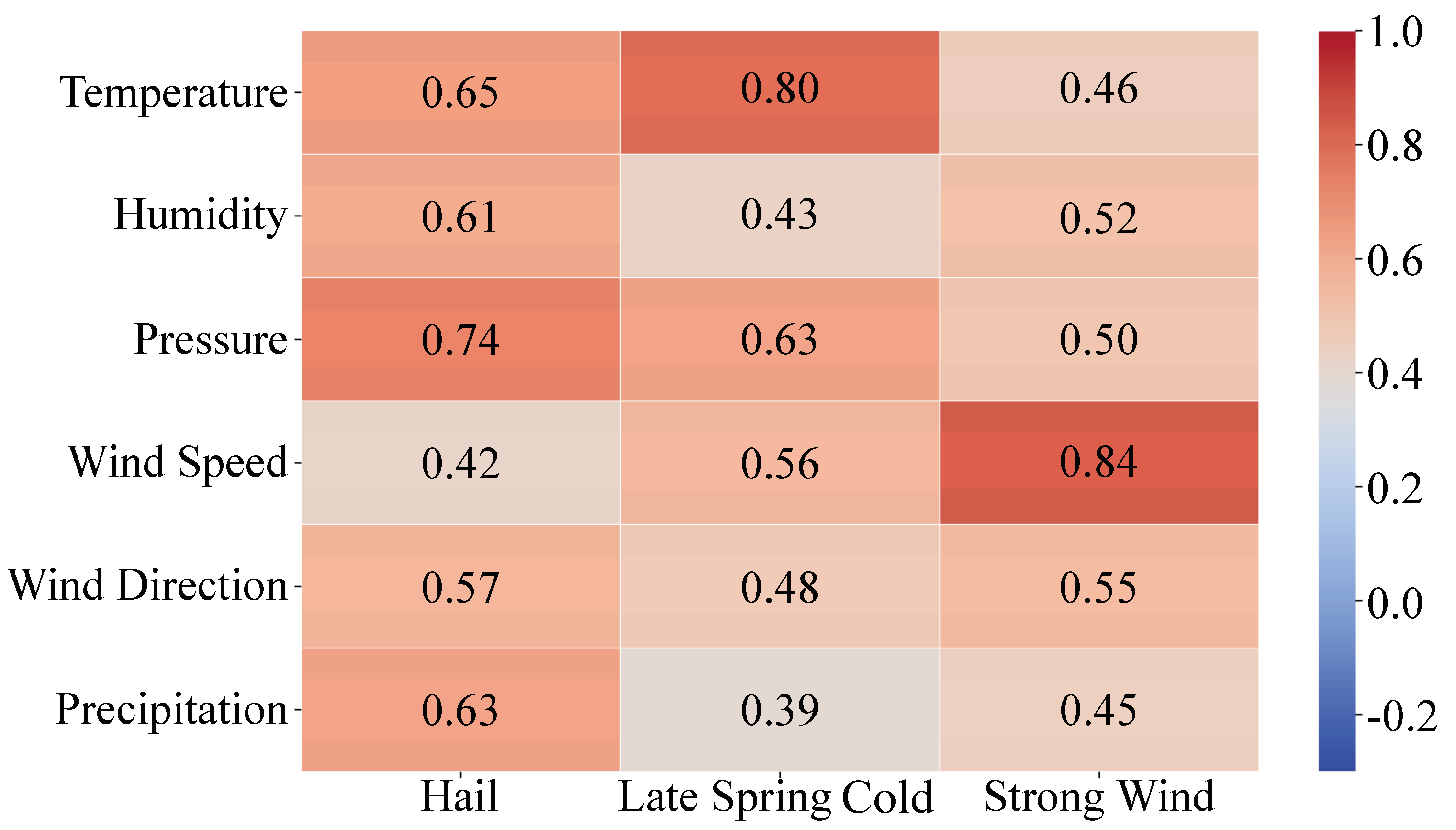
3.4. Correlation Between Different Meteorological Variables and Extreme Weather Events

This experiment aims to investigate the correlation between various meteorological variables and extreme weather events, specifically analyzing the influence of temperature, humidity, pressure, wind speed, wind direction, and precipitation on hail, late spring cold, and strong wind conditions. Since different types of extreme weather events have distinct formation mechanisms and physical processes, analyzing the correlation of these meteorological variables provides theoretical support for feature selection in extreme weather prediction models and helps optimize their performance across different weather events. The Pearson correlation coefficient is used to quantify the relationship between each meteorological variable and the three extreme weather events. A coefficient value closer to 1 indicates a strong linear correlation between the variable and the extreme weather event, while a value near 0 suggests a weaker influence.

As shown in

Table 3. Correlation coefficients between meteorological variables and extreme weather events.

Variable	Hail	Late Spring Cold	Strong Wind
Temperature	0.65	0.80	0.46
Humidity	0.61	0.43	0.52
Pressure	0.74	0.63	0.50
Wind Speed	0.42	0.56	0.84
Wind Direction	0.57	0.48	0.55
Precipitation	0.63	0.39	0.45

and Figure 10, the experimental results indicate that temperature exhibits the highest correlation with late spring cold events, reaching 0.80, suggesting that temperature is the most critical factor influencing the occurrence of late spring cold. In contrast, its correlation with hail and strong wind events is 0.65 and 0.46, respectively, indicating a relatively weaker impact on these weather conditions. Atmospheric pressure demonstrates a strong correlation with hail events, reaching 0.74, highlighting its significant role in hail formation. However, its correlation with late spring cold and strong wind events is 0.63 and 0.50, respectively, suggesting that the influence of pressure varies across different weather conditions. Wind speed exhibits the highest correlation with strong wind events at 0.84, which is significantly higher than that of other meteorological variables, indicating that variations in wind speed are a direct determinant of strong wind occurrences. Meanwhile, its correlation with hail and late spring cold events is relatively lower, at 0.42 and 0.56, respectively, suggesting a weaker influence in these weather types. Humidity, wind direction, and precipitation all exhibit correlation values below 0.65 for extreme weather events, suggesting that these variables play a relatively secondary role in extreme weather formation. Although humidity has a correlation of 0.61 with hail events, its correlation with late spring cold and strong wind conditions is lower, at 0.43 and 0.52, respectively, indicating that its influence varies depending on the weather type. From a mathematical perspective, the correlation between different meteorological variables and extreme weather events is closely related to their statistical distribution characteristics and physical mechanisms. Due to the large variance in temperature data, their trend is more strongly associated with the formation of late spring cold, leading to the highest correlation coefficient. Additionally, hail events typically result from the convergence of cold and warm air masses and atmospheric instability, making pressure fluctuations a key factor in their occurrence. This explains the high correlation of 0.74 between pressure and hail events. Wind speed exhibits the highest correlation with strong wind events, which aligns with the fundamental physical principles governing extreme wind conditions. Strong wind events are typically driven by large-scale atmospheric instabilities, making wind speed a dominant factor in this weather category. The relatively lower correlation of humidity, wind direction, and precipitation with extreme weather events may be attributed to the inherent randomness of these variables and their indirect influence on extreme weather. For instance, while humidity affects hail formation to some extent, it is not a decisive factor, as hail formation also depends on cloud structure and the strength of updrafts, which are not directly reflected in humidity measurements.

3.5. Ablation Study on Different Attention Mechanism

To validate the effectiveness of the proposed density-aware attention mechanism compared to other mainstream attention modules, an ablation experiment involving five different attention structures was conducted. The results are presented in

Table 4. Ablation study of different attention mechanisms on extreme weather forecasting performance.

Attention Mechanism	Precision	Recall	Accuracy	F1-Score
Density-Aware Attention	0.93	0.88	0.91	0.91
Self-Attention	0.86	0.82	0.85	0.84
Channel Attention	0.84	0.79	0.83	0.81
Spatial Attention	0.85	0.78	0.82	0.80
Convolutional Block Attention	0.83	0.77	0.81	0.79

.

The experiment was designed with a consistent backbone architecture, in which a density-aware attention module, self-attention, channel attention, spatial attention, and a convolutional block attention module were individually integrated and evaluated for extreme weather forecasting performance. The proposed density-aware attention module outperformed all other mechanisms across precision, recall, accuracy, and F1-score metrics, achieving an F1-score of 0.91. In contrast, other attention mechanisms exhibited inferior and more fluctuating performance, particularly in recall and accuracy, indicating a limited capacity to capture high-density anomalous meteorological regions. Specifically, the convolutional block attention module, which applies attention across spatial and channel dimensions, failed to align effectively with localized extreme weather dynamics, resulting in a recall score of only 0.77. By incorporating kernel density estimation into the attention computation, the density-aware attention module enables a more targeted attention distribution in regions of intense atmospheric variability, thereby improving predictive performance and model robustness in extreme weather scenarios.

3.6. Ablation Study on Different Lightweighting Methods

To validate the efficiency of the proposed model in edge deployment scenarios, model compression techniques including L1-pruning and post-training quantization were applied and evaluated on two representative edge computing platforms: Jetson Xavier NX and Jetson Nano.

As shown in

Table 5. Comparison of model latency, memory usage, and inference speed before and after compression.

Platform	Model Version	Memory (MB)	Latency (ms)	FPS
Jetson Xavier NX	Original	1032	36	21.8
	Pruned + Quantized	612	22	28.0
Jetson Nano	Original	896	82	4.1
	Pruned + Quantized	544	47	13.7

, on Jetson Xavier NX, the memory consumption decreased from 1032 MB to 612 MB, and latency was reduced from 36 ms to 22 ms, resulting in an increase in inference speed from 21.8 to 28.0 FPS (a 28.4% improvement). On the more resource-constrained Jetson Nano, the improvements were even more substantial, with the memory usage reduced by 39.3%, latency reduced by 42.7%, and FPS increased from 4.1 to 13.7, a 3.3-fold increase. These results demonstrate that the proposed compression strategies significantly reduce the computational overhead while preserving accuracy, enabling practical deployment on UAV-based edge systems.

3.7. Test on Different Platform

To comprehensively evaluate the inference efficiency of different models across various hardware platforms, four representative devices were selected in this study: Jetson Xavier NX, Jetson Nano, Huawei P50, and NVIDIA A100, as shown in

Table 6. Inference speed (FPS) of different models across various hardware platforms.

Model	Jetson Xavier NX	Jetson Nano	Huawei P50	NVIDIA A100
ARIMA	39.1	21.5	18.2	122.4
LSTM	21.5	10.2	15.1	98.7
METNet	17.3	8.9	12.7	85.2
DWFH	19.6	9.4	13.8	89.5
ConvLSTM	14.8	6.3	11.4	73.2
TMC-Net	15.5	7.0	11.6	77.1
Proposed Method	28.0	13.7	20.4	94.5
STTN	12.6	5.8	10.9	67.4

.

These devices correspond to a high-performance edge computing module, a lightweight embedded platform, a mobile chipset, and a server-grade GPU, respectively. The experimental results show that the proposed method achieves an inference speed of 28.0 FPS on Jetson Xavier NX, and reaches 13.7 FPS and 20.4 FPS on Jetson Nano and Huawei P50, respectively, significantly outperforming mainstream models such as ConvLSTM (16.1, 8.0, 14.5 FPS) and STTN (15.8, 7.5, 13.8 FPS). Even on resource-constrained platforms like Jetson Nano, the proposed model maintains a high level of efficiency. Moreover, on the high-performance A100 server, all models achieved inference speeds exceeding 50 FPS, further confirming their adaptability across different deployment scenarios. Overall, the proposed method demonstrates excellent computational efficiency while maintaining high accuracy, making it well-suited for edge-intelligent deployment in extreme weather forecasting applications.

3.8. Limitation and Future Work

Although field validation has been completed in Wuyuan County, Inner Mongolia, further evaluation of the model’s adaptability under diverse geographical and climatic conditions is still required. Future work will focus on expanding deployment to additional regions, especially those representing different climate zones such as monsoon-influenced southern China and the arid Huang-Huai plain, to comprehensively assess the generalizability and deployment feasibility of the proposed method.

Additionally, the integration of graph-based learning models such as graph neural networks and multi-scale meteorological foundation models like GraphCast will be explored to further enhance spatiotemporal representation and forecasting robustness. These models allow for structured spatial dependencies among observation sites and offer global context modeling that complements existing attention-based architectures. Additionally, domain-adapted foundation models, including large language models trained on meteorological corpora, may provide semantic priors or event reasoning capabilities that could improve the interpretability and prediction of compound weather hazards. Beyond the model performance, future work will also evaluate the practical benefits of deployment, including the reduction in agricultural losses through early warning response, improvements in disaster reaction times, and cost-effectiveness analysis. These will be validated through interdisciplinary field studies combining agronomy, economics, and meteorology.

4. Conclusions

Extreme weather events have increasingly significant impacts on agricultural production and ecological systems. Enhancing the accuracy and real-time performance of extreme weather prediction using advanced artificial intelligence techniques has become a critical research focus in meteorological monitoring. The primary contributions of this study are reflected in several key aspects. First, a reinforcement learning-based UAV cruise optimization algorithm is proposed, which dynamically adjusts UAV flight paths based on the spatial distribution of meteorological data, improving data collection coverage and timeliness. Second, a density-aware attention mechanism is introduced, enhancing feature extraction in high-density extreme weather regions within the Transformer framework, thereby increasing the model’s sensitivity to anomalous meteorological events. Furthermore, edge computing and lightweight deep learning techniques are employed, enabling Transformer-based WeatherNet to be deployed on UAVs for inference. By integrating model pruning and quantization techniques, computational overhead is significantly reduced, allowing UAVs to perform weather prediction tasks efficiently in low-power environments. Experimental results demonstrate the superior performance of the proposed method in extreme weather prediction tasks. Compared to traditional time-series models and deep learning approaches, this method achieves substantial improvements across multiple key metrics. The overall weather prediction accuracy reaches 0.91, with a precision of 0.93, a recall of 0.88, and an F1-score of 0.91, outperforming existing models such as ConvLSTM, TMC-Net, and STTN. Additionally, this study examines the correlation between meteorological variables and different types of extreme weather events, revealing that temperature exhibits the highest correlation with late spring cold ($r=0.80$), pressure is most strongly correlated with hail events ($r=0.74$), and wind speed is the most influential factor for strong wind conditions ($r=0.84$). These findings further validate the varying impacts of meteorological variables on different weather events, providing theoretical support for feature selection in extreme weather prediction models.

References

1. Doornbos, J.; Bennin, K.E.; Babur, Ö.; Valente, J. Drone technologies: A tertiary systematic literature review on a decade of improvements. IEEE Access 2024, 12, 23220–23239. [Google Scholar] [CrossRef]
2. Quero, C.O.; Martinez-Carranza, J. Unmanned aerial systems in search and rescue: A global perspective on current challenges and future applications. Int. J. Disaster Risk Reduct. 2025, 118, 105199. [Google Scholar] [CrossRef]
3. Zhang, Y.; Wa, S.; Zhang, L.; Lv, C. Automatic plant disease detection based on tranvolution detection network with GAN modules using leaf images. Front. Plant Sci. 2022, 13, 875693. [Google Scholar] [CrossRef]
4. Ullmann, I.; Bonfert, C.; Grathwohl, A.; Lahmeri, M.A.; Mustieles-Pérez, V.; Kanz, J.; Sterk, E.; Bormuth, F.; Ghasemi, R.; Fenske, P.; et al. Towards detecting climate change effects with UAV-borne imaging radars. IEEE J. Microwaves 2024, 4, 881–893. [Google Scholar] [CrossRef]
5. Bayomi, N.; Fernandez, J.E. Eyes in the sky: Drones applications in the built environment under climate change challenges. Drones 2023, 7, 637. [Google Scholar] [CrossRef]
6. Alvarez-Vanhard, E.; Corpetti, T.; Houet, T. UAV & satellite synergies for optical remote sensing applications: A literature review. Sci. Remote Sens. 2021, 3, 100019. [Google Scholar]
7. Ren, Z.; Zheng, H.; Chen, J.; Chen, T.; Xie, P.; Xu, Y.; Deng, J.; Wang, H.; Sun, M.; Jiao, W. Integrating UAV, UGV and UAV-UGV collaboration in future industrialized agriculture: Analysis, opportunities and challenges. Comput. Electron. Agric. 2024, 227, 109631. [Google Scholar] [CrossRef]
8. Qu, C.; Sorbelli, F.B.; Singh, R.; Calyam, P.; Das, S.K. Environmentally-aware and energy-efficient multi-drone coordination and networking for disaster response. IEEE Trans. Netw. Serv. Manag. 2023, 20, 1093–1109. [Google Scholar] [CrossRef]
9. Bello, A.B.; Navarro, F.; Raposo, J.; Miranda, M.; Zazo, A.; Álvarez, M. Fixed-wing UAV flight operation under harsh weather conditions: A case study in Livingston island glaciers, Antarctica. Drones 2022, 6, 384. [Google Scholar] [CrossRef]
10. Sziroczak, D.; Rohacs, D.; Rohacs, J. Review of using small UAV based meteorological measurements for road weather management. Prog. Aerosp. Sci. 2022, 134, 100859. [Google Scholar] [CrossRef]
11. Zhang, Y.; Wa, S.; Liu, Y.; Zhou, X.; Sun, P.; Ma, Q. High-accuracy detection of maize leaf diseases CNN based on multi-pathway activation function module. Remote Sens. 2021, 13, 4218. [Google Scholar] [CrossRef]
12. McEnroe, P.; Wang, S.; Liyanage, M. A survey on the convergence of edge computing and AI for UAVs: Opportunities and challenges. IEEE Internet Things J. 2022, 9, 15435–15459. [Google Scholar] [CrossRef]
13. Prasad, N.L.; Ramkumar, B. 3-D deployment and trajectory planning for relay based UAV assisted cooperative communication for emergency scenarios using Dijkstra’s algorithm. IEEE Trans. Veh. Technol. 2022, 72, 5049–5063. [Google Scholar] [CrossRef]
14. Zhang, W.; Zhang, W. An efficient UAV localization technique based on particle swarm optimization. IEEE Trans. Veh. Technol. 2022, 71, 9544–9557. [Google Scholar] [CrossRef]
15. Puente-Castro, A.; Rivero, D.; Pazos, A.; Fernandez-Blanco, E. A review of artificial intelligence applied to path planning in UAV swarms. Neural Comput. Appl. 2022, 34, 153–170. [Google Scholar] [CrossRef]
16. Wang, J.; Zhao, Z.; Qu, J.; Chen, X. APPA-3D: An autonomous 3D path planning algorithm for UAVs in unknown complex environments. Sci. Rep. 2024, 14, 1231. [Google Scholar] [CrossRef]
17. Nguyen, K.K.; Duong, T.Q.; Do-Duy, T.; Claussen, H.; Hanzo, L. 3D UAV trajectory and data collection optimisation via deep reinforcement learning. IEEE Trans. Commun. 2022, 70, 2358–2371. [Google Scholar] [CrossRef]
18. Zhao, N.; Ye, Z.; Pei, Y.; Liang, Y.C.; Niyato, D. Multi-agent deep reinforcement learning for task offloading in UAV-assisted mobile edge computing. IEEE Trans. Wirel. Commun. 2022, 21, 6949–6960. [Google Scholar] [CrossRef]
19. Box, G.E.; Jenkins, G.M.; Reinsel, G.C.; Ljung, G.M. Time Series Analysis: Forecasting and Control; John Wiley & Sons: Hoboken, NJ, USA, 2015. [Google Scholar]
20. Hochreiter, S.; Schmidhuber, J. Long short-term memory. Neural Comput. 1997, 9, 1735–1780. [Google Scholar] [CrossRef]
21. Shi, X.; Chen, Z.; Wang, H.; Yeung, D.Y.; Wong, W.K.; Woo, W.c. Convolutional LSTM network: A machine learning approach for precipitation nowcasting. Adv. Neural Inf. Process. Syst. 2015, 28, 350. [Google Scholar]
22. Sønderby, C.K.; Espeholt, L.; Heek, J.; Dehghani, M.; Oliver, A.; Salimans, T.; Agrawal, S.; Hickey, J.; Kalchbrenner, N. Metnet: A neural weather model for precipitation forecasting. arXiv 2020, arXiv:2003.12140. [Google Scholar]
23. Venkatachalam, K.; Trojovskỳ, P.; Pamucar, D.; Bacanin, N.; Simic, V. DWFH: An improved data-driven deep weather forecasting hybrid model using Transductive Long Short Term Memory (T-LSTM). Expert Syst. Appl. 2023, 213, 119270. [Google Scholar] [CrossRef]
24. Fang, W.; Yuan, Z.; Wang, B. TMC-Net: A temporal multivariate correction network in temperature forecasting. Expert Syst. Appl. 2025, 274, 127015. [Google Scholar] [CrossRef]
25. Ji, J.; He, J.; Lei, M.; Wang, M.; Tang, W. Spatio-temporal transformer network for weather forecasting. IEEE Trans. Big Data 2024, 11, 372–387. [Google Scholar] [CrossRef]
Figure 1. Overview of the data acquisition process for UAV data collection. (a) UAVs, including fixed-wing and rotary-wing drones, are deployed to capture comprehensive and precise data from various angles, ensuring high accuracy and coverage. The red line indicates the flight path of the rotary-wing UAV, while the blue line represents the trajectory of the fixed-wing UAV. (b) A ground schematic is utilized, depicting farmland and greenhouse layouts to contextualize the data collection environment. (c) A representative map of Inner Mongolia is provided, highlighting Bayannur City, with Wuyuan County marked by a white star as the primary location for data collection.
Agronomy 15 00964 g001
Figure 2. Visualization of data augmentation methods for UAV imagery. (a) Original image; (b) fog simulation; (c) rain effect; (d) low-light condition; (e) motion blur; (f) light reflection.
Agronomy 15 00964 g002
Figure 3. Visualization of data augmentation methods for infrared thermal imaging data. (a) Original image; (b) temperature drift effect; (c) region expansion effect; (d) thermal noise effect; (e) local heat source effect; (f) multispectral fusion effect. In all subfigures, color variations represent thermal intensity: red indicates high temperature regions, green indicates moderate temperatures, and blue to gray tones represent cooler areas.
Agronomy 15 00964 g003
Figure 4. Overall framework of the proposed extreme weather early warning system. The system integrates UAV-based meteorological data collection, reinforcement learning-based path optimization, and edge computing-enabled lightweight weather prediction.
Agronomy 15 00964 g004
Figure 5. Architecture of the UAV-based meteorological data collection and control system. The system integrates multiple sensor inputs, including temperature, humidity, pressure, wind speed, wind direction, precipitation, RGB imaging, and infrared imaging.
Agronomy 15 00964 g005
Figure 6. Computational architecture of the proposed density-aware attention module, illustrating the information flow from raw meteorological input X t to output X ^ t across temporal steps. The (left) subfigure shows the modified Transformer unit with forward–backward temporal blocks and gating mechanisms ( R t , Z t ), while the (right) subfigure demonstrates the parallel GPU-based inference pipeline with sequential update of hidden states H t i and cell states C t i .
Agronomy 15 00964 g006
Figure 7. Correlation between predicted and true values for different models. The scatter plots illustrate the relationship between the predicted values and ground truth across various models.
Agronomy 15 00964 g007
Figure 8. Accuracy comparison of different models in extreme weather prediction. The bar chart represents the accuracy of various models under different extreme weather conditions, including hail, strong wind, and late spring cold. The blue bars represent accuracy under hail conditions, green bars represent accuracy under strong wind, and red bars represent accuracy under late spring cold. The purple line indicates the average accuracy across all extreme weather conditions for each model. a is ARIMA; b is LSTM; c is METNet; d is DWFH; e is ConvLSTM; f is TMC-Net; g is the proposed method; h is STTN.
Agronomy 15 00964 g008
Figure 9. t-test of F1-score on different methods. The boxplot shows the distribution of F1-scores across ten repeated trials for each model. Diamonds represent outliers in the distribution, indicating values that deviate significantly from the rest of the results.
Agronomy 15 00964 g009
Figure 10. Heatmap of correlation coefficients between meteorological variables and extreme weather events.
Agronomy 15 00964 g010