
Relationship of Oedaleus decorus asiaticus Densities with Soil Moisture and Land Surface Temperature in Inner Mongolia, China

 ,
, 
Abstract
:1. Introduction
1.1. Threats Posed by Grasshoppers to Ecosystems
1.2. Climate Variables Affecting Grasshopper Occurrence
1.3. Main Aim of This Study
2. Material and Methods
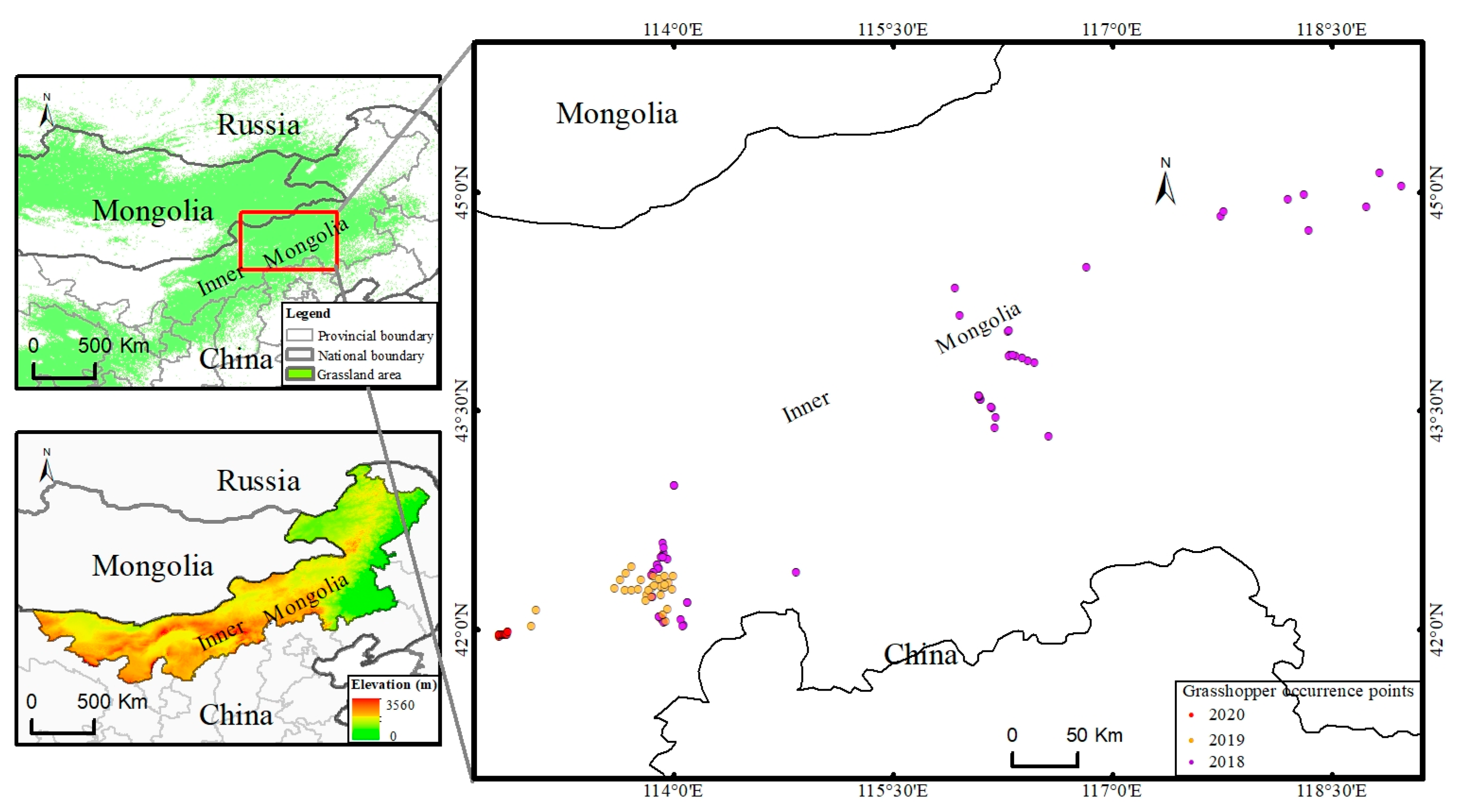
2.1. Field Experiment
2.2. SM and LST Datasets
2.3. Statistical Analyses
2.3.1. Environmental Factors and Screening
2.3.2. Generalized Additive Model
2.3.3. Optimal GAM Construction
3. Results
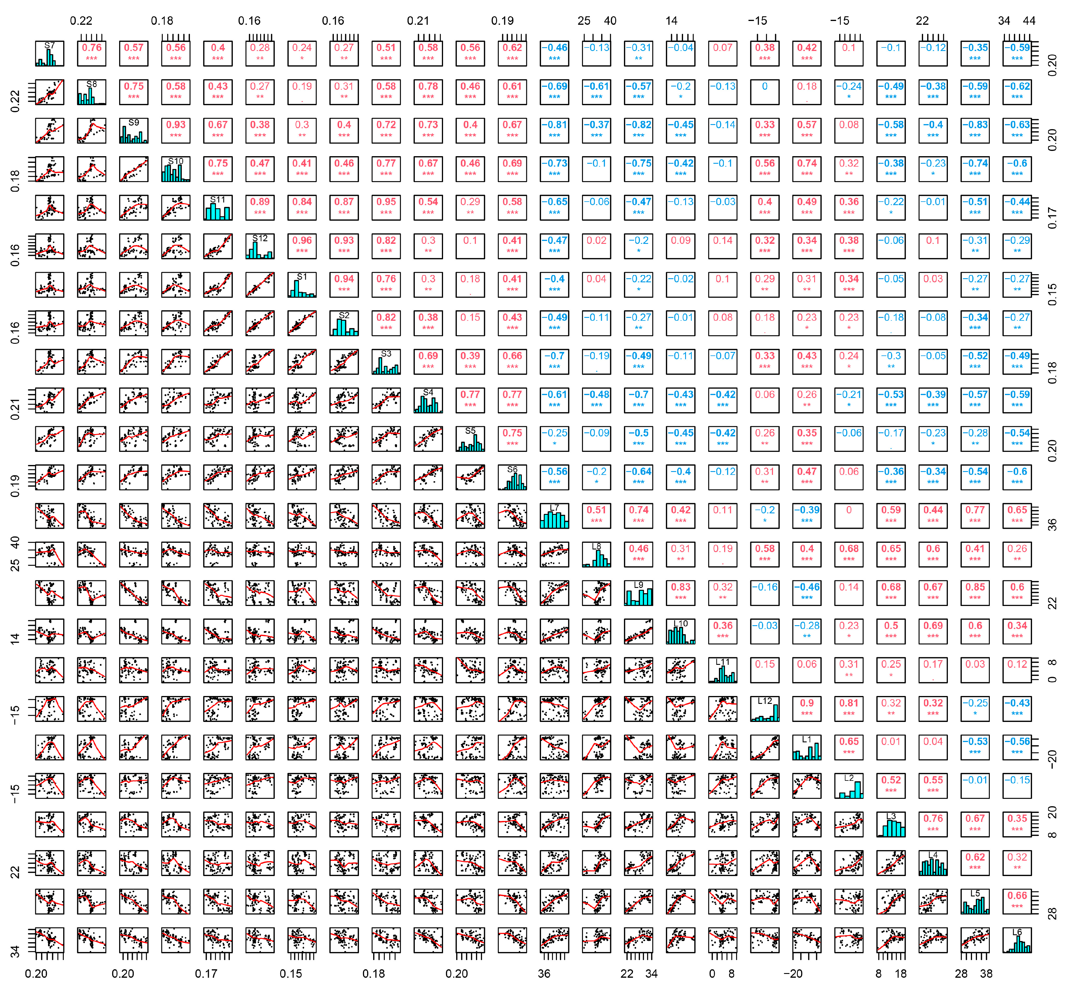
3.1. Screening of Environmental Factors
3.2. GAM Validation
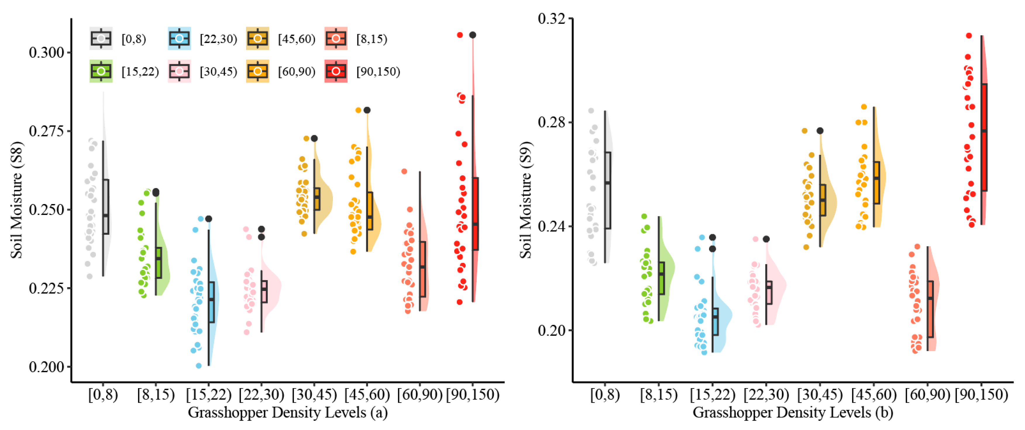
3.3. Relationship Between O. decorus Density and Monthly Average SM and LST
3.4. Roles of SM and LST in O. decorus Densities
3.4.1. Relationship Between O. decorus Densities and Daily SM
3.4.2. Relationship Between O. decorus Densities and Daily LST
4. Discussion
4.1. Role of Environmental Factors in the GAM
4.2. Influence of Environmental Factors on O. decorus Density
4.3. Recommendations for O. decorus Prediction and Monitoring
5. Conclusions
Author Contributions
Funding
Data Availability Statement
Conflicts of Interest
References
- Kang, L.; Chen, Y.L. An Approach on The Strategies of Locusts and Grasshoppers Disasters Reduction. Disasters Reduct. China 1992, 2, 50–53. [Google Scholar]
- Liu, J.P.; Xi, R.H.; Chen, Y.L. A preliminary study for oviposition preference of locusts. Entomol. Knowl. 1984, 21, 204–207. [Google Scholar]
- Du, B.B.; Ding, X.; Ji, C.; Lin, K.J.; Guo, J.; Lu, L.H.; Dong, Y.Y.; Huang, W.J.; Wang, N. Estimating Leymus Chinensis Loss Caused by Oedaleus Asiaticus Using Unmanned Aerial Vehicles (UAV). Remote Sens. 2023, 15, 4352. [Google Scholar] [CrossRef]
- Latchininsky, A.V. Locusts and Remote Sensing: A Review. J. Appl. Remote Sens. 2013, 7, 075099. [Google Scholar] [CrossRef]
- Escorihuela, M.J.; Merlin, O.; Stefan, V.; Moyano, G.; Eweys, O.A.; Zribi, M.; Kamara, S.; Benahi, A.S.; Ebbe, M.A.B.; Chihrane, J.; et al. SMOS Based High Resolution Soil Moisture Estimates for Desert Locust Preventive Management. Remote Sens. Appl. Soc. Environ. 2018, 11, 8275–8278. [Google Scholar]
- Waldner, F.; Ebbe, M.A.B.; Cressman, K.; Defourny, P. Operational Monitoring of the Desert Locust Habitat with Earth Observation: An Assessment. ISPRS Int. J. Geo-Inf. 2015, 4, 2379–2400. [Google Scholar] [CrossRef]
- Gomez, D.; Salvador, P.; Sanz, J.; Casanova, C.; Taratiel, D.; Casanova, J.L. Machine Learning Approach to Locate Desert Locust Breeding Areas Based on ESA CCI Soil Moisture. J. Appl. Remote Sens. 2018, 12, 1. [Google Scholar] [CrossRef]
- Wang, B.; Deveson, E.D.; Waters, C.; Spessa, A.; Lawton, D.; Feng, P.; Li Liu, D. Future Climate Change Likely to Reduce the Australian Plague Locust (Chortoicetes terminifera) Seasonal Outbreaks. Sci. Total Environ. 2019, 668, 947–957. [Google Scholar] [CrossRef]
- Sivanpillai, R.; Latchininsky, A.V. Special Section Guest Editorial: Advances in Remote Sensing Applications for Locust Habitat Monitoring and Management. J. Appl. Remote Sens. 2015, 8, 084801. [Google Scholar] [CrossRef]
- Shi, Y.; Huang, W.; Dong, Y.; Peng, D.; Zheng, Q.; Yang, P. The Influence of Landscape’s Dynamics on the Oriental Migratory Locust Habitat Change Based on The Time-Series Satellite Data. J. Environ. Manag. 2018, 218, 280–290. [Google Scholar] [CrossRef]
- Qiu, S.B.; Lin, H.L.; Jiang, Y.H. The Study on the Relationship of the Declining Distribution and Activities of Locusts with plant Growth. Acta Phytophylacica Sin. 1962, 1, 17–22. [Google Scholar]
- Cressman, K. Role of Remote Sensing in Desert Locust Early Warning. J. Appl. Remote Sens. 2013, 7, 075098. [Google Scholar] [CrossRef]
- Meynard, C.N.; Lecoq, M.; Chapuis, M.; Piou, C. On the Relative Role of Climate Change and Management in the Current Desert Locust Outbreak in East Africa. Glob. Change Biol. 2020, 26, 3753–3755. [Google Scholar] [CrossRef] [PubMed]
- Mariottini, Y.; Marinelli, C.; Cepeda, R.; DeWysiecki, M.L.; Lange, C.E. Relationship between pest grasshopper densities and climate variables in the southern Pampas of Argentina. Bull. Entomol. Res. 2022, 112, 613–625. [Google Scholar] [CrossRef]
- Liu, Z.; Shi, X.; Warner, E.; Ge, Y.; Yu, D.; Ni, S.; Wang, H. Relationship between oriental migratory locust plague and soil moisture extracted from MODIS data. Int. J. Appl Earth Obs. Geoinf. 2008, 10, 84–91. [Google Scholar] [CrossRef]
- Geng, Y. Remote Sensing Extraction and Spatial-Temporal Evolution of Oriental Migratory Locust Potential Distribution; Aerospace Information Research Institute, Chinese Academy of Sciences: Beijing, China, 2022. [Google Scholar]
- Sun, Z.X.; Ye, H.C.; Huang, W.J.; Qimuge, E.; Zhang, Y. Application of MaxEnt and Remote Sensing Technology in Grassland Locust Disaster Risk Monitoring: An Example from the Agricultural Heritage Systems of East Ujimgin Banner. J. Ecol. Rural Environ. 2022, 38, 1265–1272. [Google Scholar]
- Wang, L.; Zhuo, W.; Pei, Z.; Tong, X.; Han, W.; Fang, S. Using Long-Term Earth Observation Data to Reveal the Factors Contributing to the Early 2020 Desert Locust Upsurge and the Resulting Vegetation Loss. Remote Sens. 2021, 13, 680. [Google Scholar] [CrossRef]
- Ma, J.W.; Han, X.Z.; Ha, S.B.G.; Wang, Z.G.; Yan, S.X.; Dai, J. Remote Sensing New Model for Monitoring the East Asian Migratory Locust Infections Based on Its Breeding Circle. J. Remote Sens. 2004, 8, 370–377. [Google Scholar]
- He, K. Assessment of Habitat Suitability for Grasshopper Using Multi-Source Fusion Data in Inner Mongolia. Master’s Thesis, Zhejiang University, Hangzhou, China, 2018. [Google Scholar]
- Kong, H.H.; Lu, W.S.; Lv, G.Q.; Wang, X.D.; Wang, J.J. Effect of Drought and Higher Temperature on the Outbreaks of the Oriental Migratory Locust in Henan Province. J. Nanjing Inst. Meteorol. 2003, 26, 516–524. [Google Scholar]
- Powell, L.R.; Berg, A.A.; Johnson, D.L.; Warland, J.S. Relationships of Pest Grasshopper Populations in Alberta, Canada to Soil Moisture and Climate Variables. Agric. For. Meteorol. 2007, 144, 73–84. [Google Scholar] [CrossRef]
- Tian, H.; Stige, L.C.; Cazelles, B.; Kausrud, K.L.; Svarverud, R.; Stenseth, N.C.; Zhang, Z. Reconstruction of a 1910-y-long Locust Series Reveals Consistent Associations with Climate Fluctuations in China. Proc. Natl. Acad. Sci. USA 2011, 108, 14521–14526. [Google Scholar] [CrossRef] [PubMed]
- Gage, S.H.; Mukerji, M.K. A Perspective of Grasshopper Population Distribution in Saskatchewan and Interrelationship with Weather. Environ. Entomol. 1977, 6, 469–479. [Google Scholar] [CrossRef]
- Capinera, J.L.; Horton, D.R. Geographic Variation in Effects of Weather on Grasshopper Infestation. Environ. Entomol. 1989, 18, 8–14. [Google Scholar] [CrossRef]
- Yu, G.; Shen, H.; Liu, J. Impacts of Climate Change on Historical Locust Outbreaks in China. J. Geophys. Res. Atmos. 2009, 114, D18104. [Google Scholar] [CrossRef]
- Loew, F.; Waldner, F.; Latchininsky, A.; Biradar, C.; Bolkart, M.; Colditz, R.R. Timely Monitoring of Asian Migratory Locust Habitats in the Amudarya Delta, Uzbekistan Using Time Series of Satellite Remote Sensing Vegetation Index. J. Environ. Manag. 2016, 183, 562–575. [Google Scholar] [CrossRef] [PubMed]
- Peng, W.; Ma, N.L.; Zhang, D.; Zhou, Q.; Yue, X.; Khoo, S.C.; Yang, H.; Guan, R.; Chen, H.; Zhang, X.; et al. A Review of Historical and Recent Locust Outbreaks: Links to Global Warming, Food Security and Mitigation Strategies. Environ. Res. 2020, 191, 110046. [Google Scholar] [CrossRef]
- Wu, T.j.; Hao, S.G.; Kang, L. Effects of Soil Temperature and Moisture on the Development and Survival of Grasshopper Eggs in Inner Mongolian Grasslands. Front. Ecol. Evol. 2021, 9, 727911. [Google Scholar] [CrossRef]
- Cease, A.J.; Elser, J.J.; Fenichel, E.P.; Hadrich, J.C.; Harrison, J.F.; Robinson, B.E. Living with Locusts: Connecting Soil Nitrogen, Locust Outbreaks, Livelihoods, and Livestock Markets. BioScience 2015, 65, 551–558. [Google Scholar] [CrossRef]
- Yang, N.; Cui, X. Study on Locust Disaster Monitoring Based on SMOS L2 Soil Moisture Data. In Proceedings of the 2019 IEEE International Geoscience and Remote Sensing Symposium, Yokohama, Japan, 28 July–2 August 2019; pp. 9413–9415. [Google Scholar]
- Guan, J.Q.; Wei, Z.Z. Determination of Food Intake of Oedaleus Decorus Asiaticus. Entomology 1989, 26, 8–10. [Google Scholar]
- Jiang, X.; Mai, M.T.M.; Zhang, L. Nocturnal Migration of Grasshopper (Acrididae: Oedaleus asiaticus). Acta Agrestia Sin. 2003, 11, 75–77. [Google Scholar]
- Zheng, X.; Song, P.; Li, Y.; Zhang, K.; Zhang, H.; Liu, L.; Huang, J. Monitoring Locusta Migratoria Manilensis Damage Using Ground Level Hyperspectral Data. In Proceedings of the 2019 8th International Conference on Agro-Geoinformatics, Istanbul, Turkey, 16–19 July 2019; pp. 1–5. [Google Scholar]
- Song, P.; Zhang, Y.; Guo, J.; Shi, J.; Zhao, T.; Tong, B. A 1 km Daily Surface Soil Moisture Dataset of Enhanced Coverage Under All-Weather Conditions over China in 2003–2019. Earth Syst. Sci. Data 2022, 14, 2613–2637. [Google Scholar] [CrossRef]
- Zhang, X.; Zhou, J.; Liang, S.; Wang, D. A Practical Reanalysis Data and Thermal Infrared Remote Sensing Data Merging (RTM) Method for Reconstruction of a 1-km All-Weather Land Surface Temperature. Remote Sens. Environ. 2021, 260, 112437. [Google Scholar] [CrossRef]
- Lu, L.H.; Kong, W.P.; Eerdengqimuge; Ye, H.C.; Sun, Z.X.; Wang, N.; Du, B.; Zhou, Y.T.; Wei, J.; Huang, W.J. Detecting Key Factors of Grasshopper Occurrence in Typical Steppe and Meadow Steppe by Integrating Machine Learning Model and Remote Sensing Data. Insects 2022, 13, 894. [Google Scholar] [CrossRef] [PubMed]
- Ou, Y.F.; Ge, F. Nonlinear Analysis of Insect Population Dynamics Based on Generalized Additive Models and Statistical Computing Using R. Chin. J. Appl. Entomol. 2013, 50, 1170–1177. [Google Scholar]
- Xu, L.; Liu, Q.; Stige, L.C.; BenAri, T.; Fang, X.; Chan, K.S.; Wang, S.; Stenseth, N.C.; Zhang, Z. Nonlinear Effect of Climate on Plague During the Third Pandemic in China. Proc. Natl. Acad. Sci. USA 2011, 108, 10214–10219. [Google Scholar] [CrossRef]
- Fartmann, T.; Poniatowski, D.; Holtmann, L. Habitat Availability and Climate Warming Drive Changes in the Distribution of Grassland Grasshoppers. Agric. Ecosyst. Environ. 2021, 320, 107565. [Google Scholar] [CrossRef]
- Singh, T.V.K. Climate Change and its Impact on Agricultural Pests. Indian J. Ecol. 2023, 50, 1874–1880. [Google Scholar]
- Ma, S.J. Formation and Reconstruction of Oriental Miaratory Locust Location. J. Intearative Aaricult. 1960, 4, 18–22. [Google Scholar]
- Li, D.; Gan, H.; Li, X.; Zhou, H.; Zhang, H.; Liu, Y.; Dong, R.; Hua, L.; Hu, G. Changes in the Range of Four Advantageous Grasshopper Habitats in the Hexi Corridor under Future Climate Conditions. Insects 2024, 15, 243. [Google Scholar] [CrossRef]
- Qi, X.L.; Wang, X.H.; Xu, H.F.; Kang, L. Influence of Soil Moisture on Egg Cold Hardiness in the Migratory Locust Locusta Migratoria (Orthoptera: Acridiidae). Physiol. Entomol. 2007, 32, 219–224. [Google Scholar] [CrossRef]
- Hunter, D. World’s Best Practice Locust and Grasshopper Management: Accurate Forecasting and Early Intervention Treatments Using Reduced Chemical Pesticide. Agronomy 2024, 14, 2369. [Google Scholar] [CrossRef]
- Veran, S.; Simpson, S.J.; Sword, G.A.; Deveson, E.; Piry, S.; Hines, J.E.; Berthier, K. Modeling Spatiotemporal Dynamics of Outbreaking Species: Influence of Environment and Migration in A Locust. Ecology 2015, 96, 737–748. [Google Scholar] [CrossRef] [PubMed]
- Wang, R.; Wu, N.; Shi, Z.; Li, C.; Jiang, N.; Fu, C.; Wang, M. Biomod2 for Evaluating the Changes in the Spatiotemporal Distribution of Locusta Migratoria Tibetensis Chen in the Qinghai-Tibet Plateau under Climate Change. Glob. Ecol. Conserv. 2025, 58, e03508. [Google Scholar] [CrossRef]
- Gao, X.M.; Ji, R. Advances in High-temperature Tolerance of Locusts and Its Mechanism. J. Plant Prot. 2022, 49, 450–459. [Google Scholar]
- Branson, D.H. Effects of Altered Seasonality of Precipitation on Grass Production and Grasshopper Performance in a Northern Mixed Prairie. Environ. Entomol. 2017, 46, 589–594. [Google Scholar] [CrossRef]
- Liu, L.; Guo, A.H. Analysis of Meteorological and Ecological Conditions of Grasshopper Infestation in Inner Mongolia in 2004. Meteorol. Mon. 2004, 30, 55–57. [Google Scholar]
- Belovsky, G.E.; Slade, J.B. Dynamics of 2 Montana Grasshopper Populations: Relationships Among Weather, Food Abundance and Intraspecific Competition. Oecologia 1995, 101, 383–396. [Google Scholar] [CrossRef]
- Huang, W.J.; Dong, Y.Y.; Zhao, L.L.; Geng, Y.; Ruan, C.; Zhang, B.Y.; Sun, Z.X.; Zhang, H.S.; Ye, H.C.; Wang, K. Review of Locust Remote Sensing Monitoring and Early Warning. J. Remote Sens. 2020, 24, 1270–1279. [Google Scholar] [CrossRef]

| Species Density/m2 | Number of Survey Sites | Cumulative Survey Sites | ||
|---|---|---|---|---|
| 2018 | 2019 | 2020 | ||
| [0, 8) | 9 | 9 | 4 | 22 |
| [8, 15) | 23 | 1 | 2 | 26 |
| [15, 22) | 0 | 1 | 19 | 20 |
| [22, 30) | 10 | 2 | 0 | 12 |
| [30, 45) | 7 | 1 | 2 | 10 |
| [45, 60) | 1 | 3 | 5 | 9 |
| [60, 90) | 0 | 2 | 1 | 3 |
| [90, 150) | 0 | 5 | 0 | 5 |
| Month | Soil Moisture | Land Surface Temperature |
|---|---|---|
| July of the year preceding the year | S7 | L7 |
| August of the year preceding the year | S8 | L8 |
| September of the year preceding the year | S9 | L9 |
| October of the year preceding the year | S10 | L10 |
| November of the year preceding the year | S11 | L11 |
| December of the year preceding the year | S12 | L12 |
| January of the year | S1 | L1 |
| February of the year | S2 | L2 |
| March of the year | S3 | L3 |
| April of the year | S4 | L4 |
| May of the year | S5 | L5 |
| June of the year | S6 | L6 |
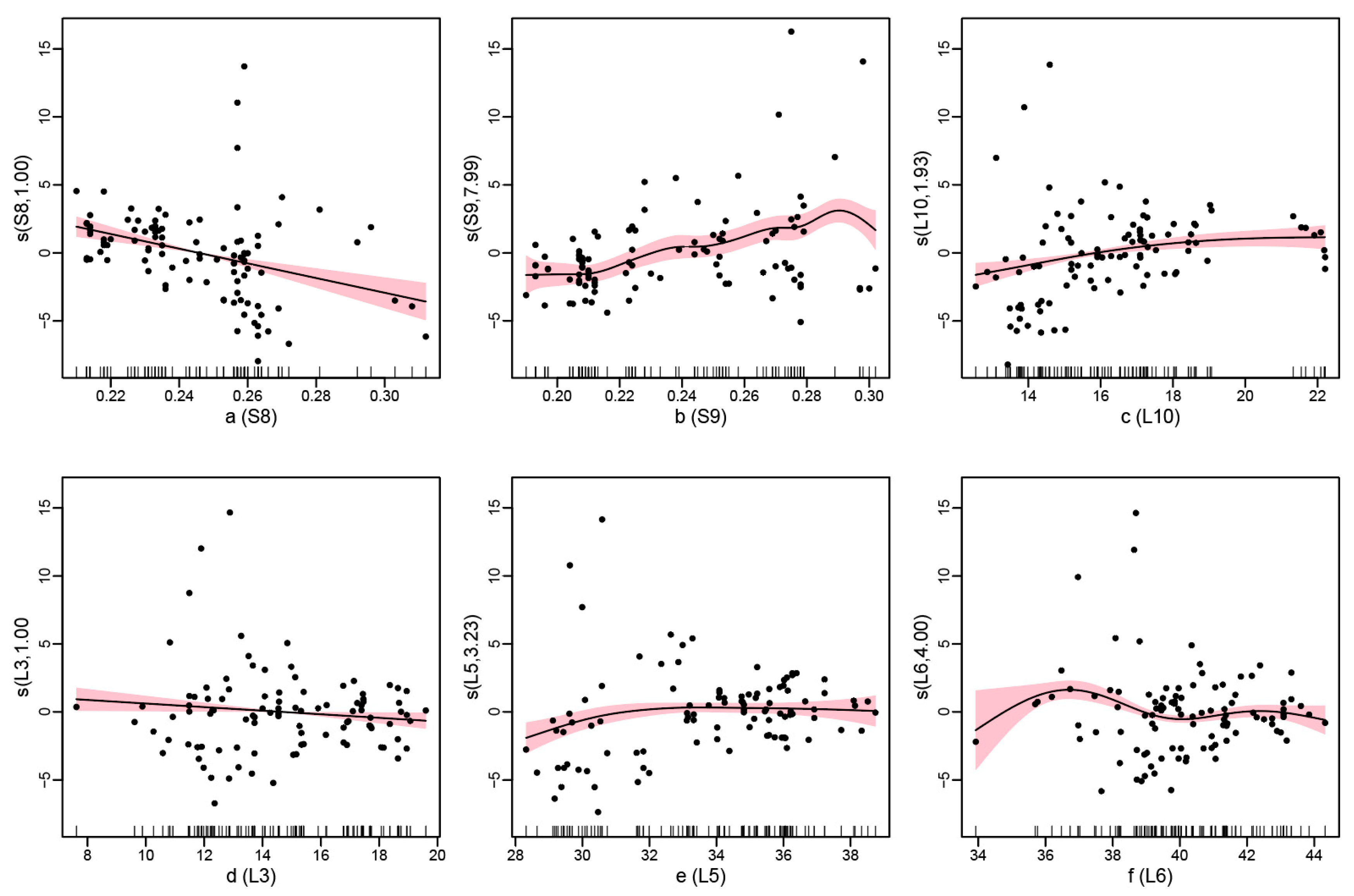
| Smoothing Effect Term | Estimated Degree of Freedom (edf) | Reference Degrees of Freedom (rdf) | F | P |
|---|---|---|---|---|
| S8 | 1.000 | 1.000 | 27.422 | 1.43 × 10⁻⁶ *** |
| S9 | 7.993 | 9.598 | 5.823 | 2.69 × 10⁻⁶ *** |
| L10 | 1.929 | 2.433 | 7.848 | 0.000445 *** |
| L3 | 1.000 | 1.000 | 4.919 | 0.029360 * |
| L5 | 3.226 | 4.052 | 3.547 | 0.012227 * |
| L6 | 4.000 | 4.000 | 7.223 | 4.97 × 10⁻⁵ *** |
Disclaimer/Publisher’s Note: The statements, opinions and data contained in all publications are solely those of the individual author(s) and contributor(s) and not of MDPI and/or the editor(s). MDPI and/or the editor(s) disclaim responsibility for any injury to people or property resulting from any ideas, methods, instructions or products referred to in the content. |
© 2025 by the authors. Licensee MDPI, Basel, Switzerland. This article is an open access article distributed under the terms and conditions of the Creative Commons Attribution (CC BY) license (https://creativecommons.org/licenses/by/4.0/).
Share and Cite
Du, B.; Shan, Y.; Huang, W.; Dong, Y.; Gao, S.; Yue, Y.; Guo, J.; Ga, L.; Zhang, Y.; Han, H. Relationship of Oedaleus decorus asiaticus Densities with Soil Moisture and Land Surface Temperature in Inner Mongolia, China. Agronomy 2025, 15, 998. https://doi.org/10.3390/agronomy15040998
Du B, Shan Y, Huang W, Dong Y, Gao S, Yue Y, Guo J, Ga L, Zhang Y, Han H. Relationship of Oedaleus decorus asiaticus Densities with Soil Moisture and Land Surface Temperature in Inner Mongolia, China. Agronomy. 2025; 15(4):998. https://doi.org/10.3390/agronomy15040998
Chicago/Turabian StyleDu, Bobo, Yanmin Shan, Wenjiang Huang, Yingying Dong, Shujing Gao, Yuchao Yue, Jing Guo, Liwa Ga, Yan Zhang, and Haibin Han. 2025. "Relationship of Oedaleus decorus asiaticus Densities with Soil Moisture and Land Surface Temperature in Inner Mongolia, China" Agronomy 15, no. 4: 998. https://doi.org/10.3390/agronomy15040998
APA StyleDu, B., Shan, Y., Huang, W., Dong, Y., Gao, S., Yue, Y., Guo, J., Ga, L., Zhang, Y., & Han, H. (2025). Relationship of Oedaleus decorus asiaticus Densities with Soil Moisture and Land Surface Temperature in Inner Mongolia, China. Agronomy, 15(4), 998. https://doi.org/10.3390/agronomy15040998