Aerosol Optical Properties and Contribution to Differentiate Haze and Haze-Free Weather in Wuhan City


 ,
,  , and
, and 
Abstract
:1. Introduction
2. Experimental Methodology
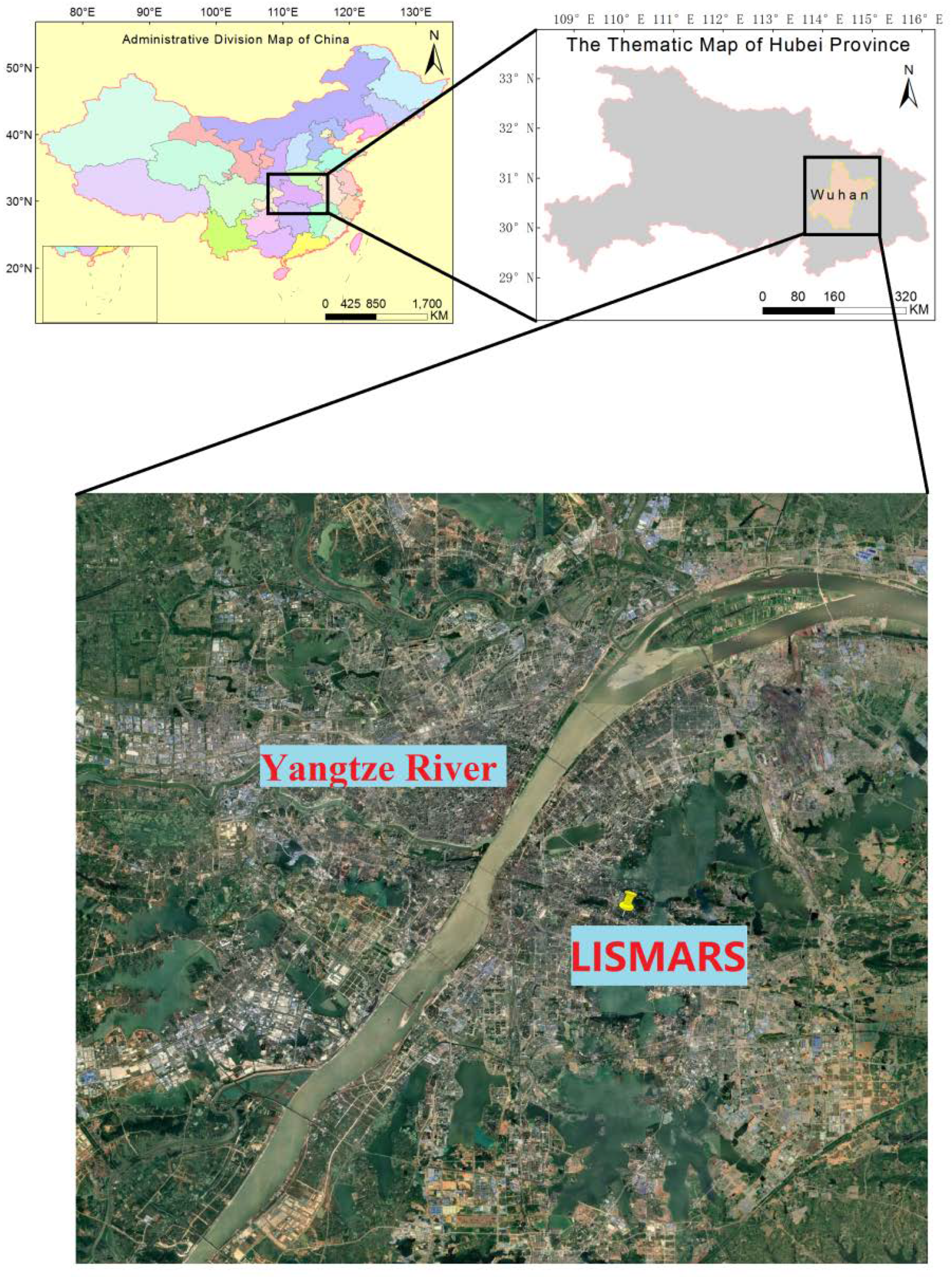
2.1. Study Area, Equipment and Data
2.2. Methodology
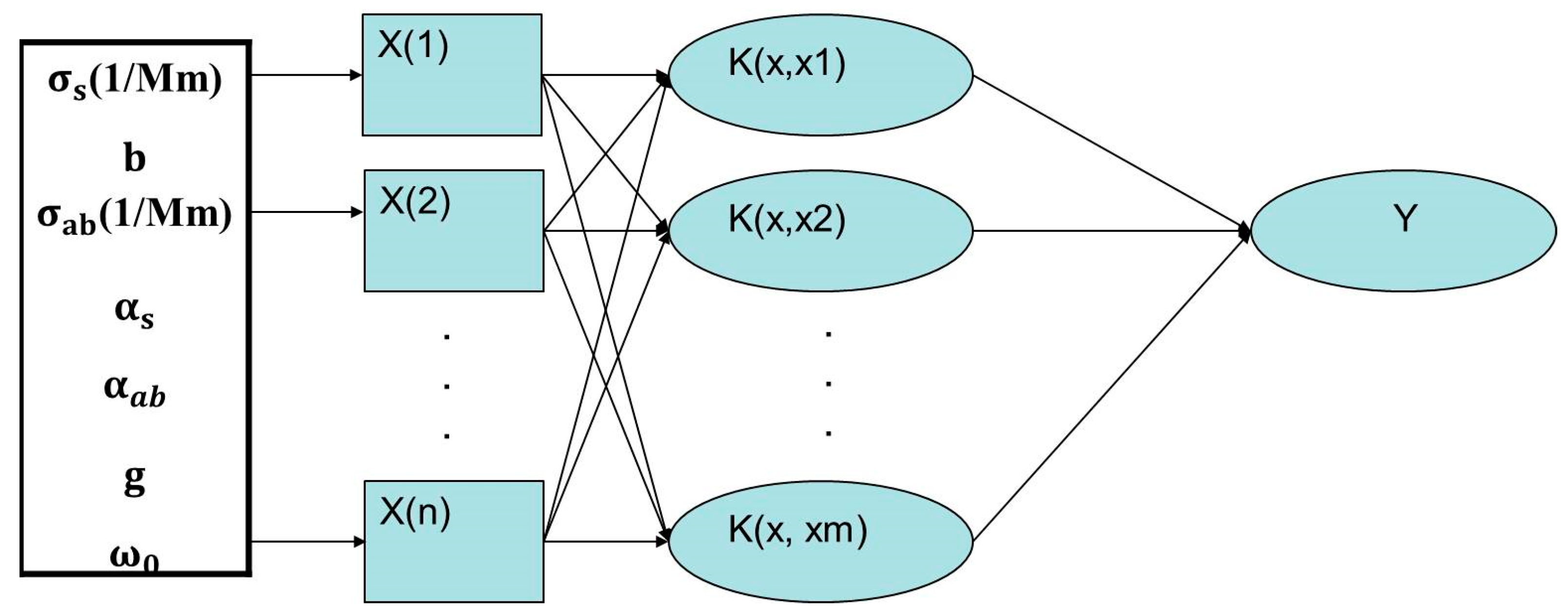
2.3. Support Vector Machine Algorithm
3. Results and Discussion
3.1. Overview of Aerosol Scattering and Absorption Properties
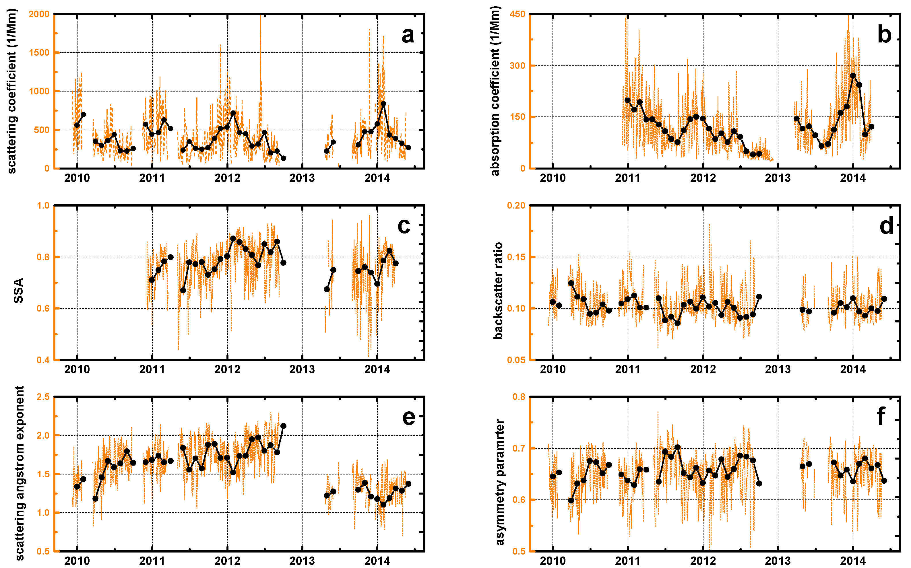
3.2. Seasonal Variation of Aerosol Scattering and Absorption Properties
3.3. SVM Results
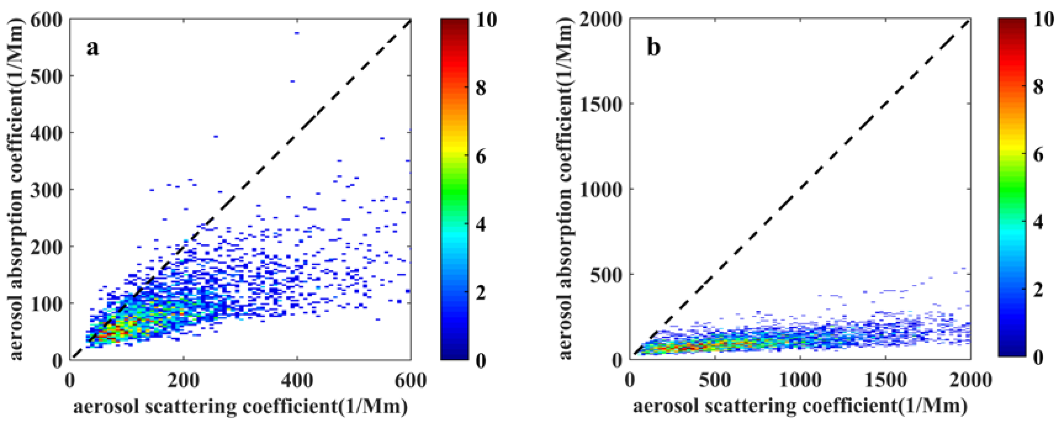
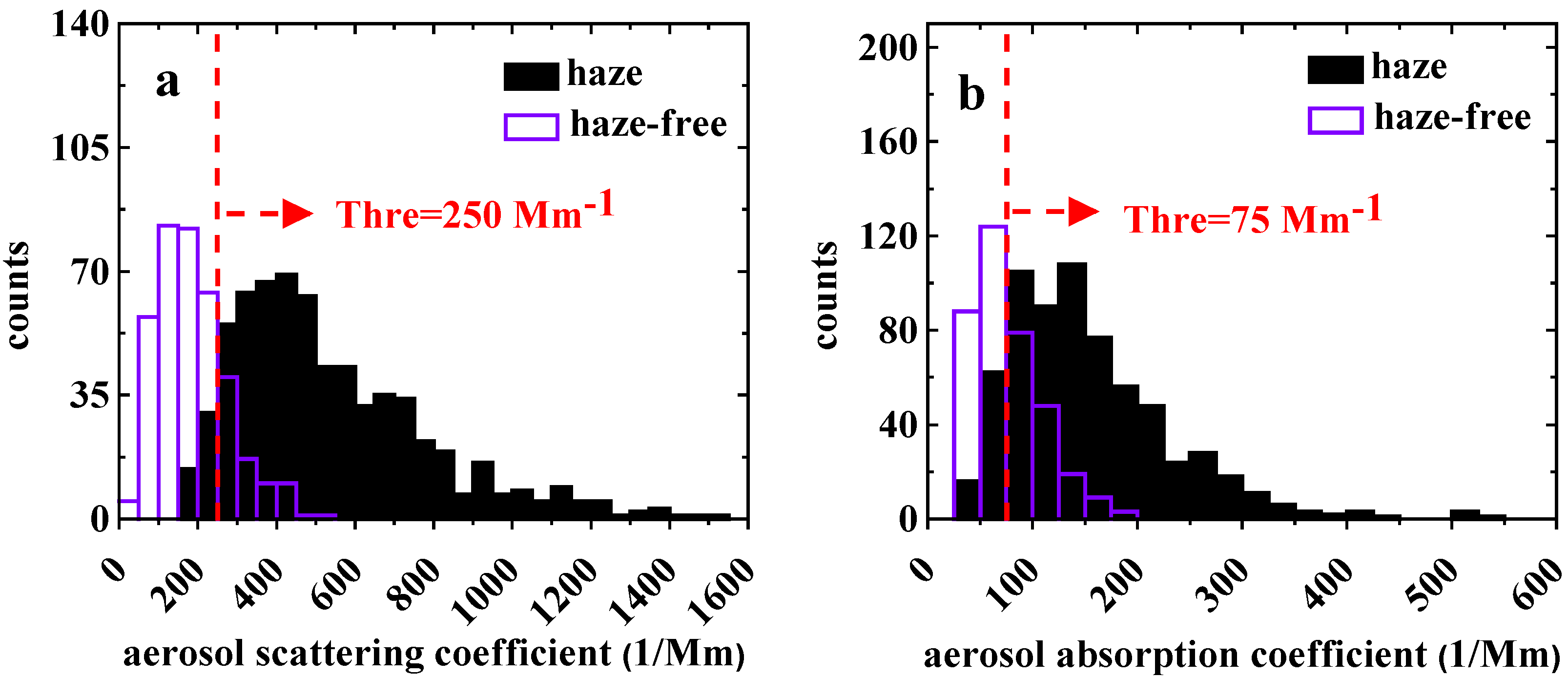
- (1)
- For σs > 250 Mm−1 and σab > 75 Mm−1, the aerosols are identified as haze aerosols.
- (2)
- For σs < 250 Mm−1 but σab > 75 Mm−1, the aerosols are also identified as haze aerosols.
- (3)
- For σab < 75 Mm−1 but σs > 250 Mm−1, the aerosols are also identified as haze aerosols.
- (4)
- For σs < 250 Mm−1 and σab < 75 Mm−1, the aerosols are identified as haze-free aerosols. We used this new standard to identify haze aerosols from our database, and the detection accuracy was 81.49%, indicating that the standard was suitable to distinguish between haze and haze-free aerosols in Wuhan City.
4. Conclusions
Author Contributions
Funding
Acknowledgments
Conflicts of Interest
References
- Hinds, W.C. Aerosol technology. Wiley Sons 2000, 31, 175. [Google Scholar]
- Gong, W.; Zhang, M.; Han, G.; Ma, X.; Zhu, Z. An investigation of aerosol scattering and absorption properties in wuhan, central china. Atmosphere 2015, 6, 503–520. [Google Scholar] [CrossRef] [Green Version]
- Zhang, M.; Ma, Y.; Gong, W.; Zhu, Z. Aerosol optical properties of a haze episode in wuhan based on ground-based and satellite observations. Atmosphere 2014, 5, 699–719. [Google Scholar] [CrossRef] [Green Version]
- Zhang, M.; Wang, L.; Bilal, M.; Gong, W.; Zhang, Z.; Guo, G. The characteristics of the aerosol optical depth within the lowest aerosol layer over the tibetan plateau from 2007 to 2014. Remote Sens. 2018, 10, 696. [Google Scholar] [CrossRef] [Green Version]
- Markku, K.; Jenni, K.; Heikki, J.; Katrianne, L.; Manninen, H.E.; Tuomo, N.; Tuukka, P.J.; Mikko, S.; Siegfried, S.; Pekka, R. Direct observations of atmospheric aerosol nucleation. Science 2013, 339, 943–946. [Google Scholar]
- Mcmurry, P.H. A review of atmospheric aerosol measurements. Atmos. Environ. 2000, 34, 1959–1999. [Google Scholar] [CrossRef]
- Magistrale, P.V. Health Aspects of Air Pollution; Springer: Berlin/Heidelberg, Germany, 1992; pp. 25–31. [Google Scholar]
- Tie, X.; Wu, D.; Brasseur, G. Lung cancer mortality and exposure to atmospheric aerosol particles inguangzhou, china. Atmos. Environ. 2009, 43, 2375–2377. [Google Scholar] [CrossRef]
- Edenhofer, O. Climate Change 2014: Mitigation of Climate Change: Working Group III Contribution to the Fifth Assessment Report of the Intergovernmental Panel on Climate Change; Cambridge University Press: Cambridge, UK, 2014. [Google Scholar]
- Rosenfeld, D. Suppression of rain and snow by urban and industrial air pollution. Int. J. Food Microbiol. 2000, 287, 40–50. [Google Scholar] [CrossRef] [PubMed]
- Twomey, S. The influence of pollution on the shortwave albedo of clouds. J. Atmos. Sci. 1977, 34, 1149–1154. [Google Scholar] [CrossRef] [Green Version]
- Parrish, D.D.; Tong, Z. Climate change. Clean air for megacities. Science 2009, 326, 674–675. [Google Scholar] [CrossRef]
- Vautard, R.; Yiou, P.; Oldenborgh, G.J.V. Decline of fog, mist and haze in europe over the past 30 years. Nat. Geosci. 2009, 2, 115–119. [Google Scholar] [CrossRef]
- Quan, J.; Zhang, Q.; He, H.; Liu, J.; Huang, M.; Jin, H. Analysis of the formation of fog and haze in north china plain (ncp). Atmos. Chem. Phys. 2011, 11, 8205–8214. [Google Scholar] [CrossRef] [Green Version]
- Xu, J.; Tao, J.; Zhang, R.; Cheng, T.; Leng, C.; Chen, J.; Huang, G.; Li, X.; Zhu, Z. Measurements of surface aerosol optical properties in winter of shanghai. Atmos. Res. 2012, 109–110, 25–35. [Google Scholar] [CrossRef]
- Lijie, H.; Lunche, W.; Aiwen, L.; Ming, Z.; Xiangao, X.; Minghui, T.; Hao, Z. What drives changes in aerosol properties over the Yangtze River basin in past four decades? Atmos. Environ. 2018, 190, 269–283. [Google Scholar]
- Shen, X.L.; Dang, T.G.; Liu, J. Summary of beijing-tianjin-hebei haze causes and solutions research. Adv. Mater. Res. 2014, 1010–1012, 639–644. [Google Scholar] [CrossRef]
- Tao, M.; Chen, L.; Lin, S.; Tao, J. Satellite observation of regional haze pollution over the north china plain. J. Geophys. Res. Atmos. 2012, 117. [Google Scholar] [CrossRef]
- Huang, J.; Zhang, W.; Zuo, J.; Jianrong, B.I.; Shi, J.; Wang, X.; Chang, Z.; Huang, Z.; Yang, S.; Zhang, S. An overview of the semi-arid climate and environment research observatory over the loess plateau. Adv. Atmos. Sci. 2008, 25, 906. [Google Scholar] [CrossRef]
- Yan, W.; Che, H.; Ma, J.; Qiang, W.; Shi, G.; Chen, H.; Goloub, P.; Hao, X. Aerosol radiative forcing under clear, hazy, foggy, and dusty weather conditions over Beijing, China. Geophys. Res. Lett. 2009, 36, 150–164. [Google Scholar]
- Ramanathan, V.; Chung, C.; Kim, D.; Bettge, T.; Buja, L.; Kiehl, J.T.; Washington, W.M.; Fu, Q.; Sikka, D.R.; Wild, M. Atmospheric brown clouds: Impacts on south Asian climate and hydrological cycle. Proc. Natl. Acad. Sci. USA 2005, 102, 5326–5333. [Google Scholar] [CrossRef] [Green Version]
- Xia, X.; Chen, H.B.; Wang, P.C.; Zhang, W.X.; Holben, B.N. Variation of column-integrated aerosol properties in a Chinese urban region. J. Geophys. Res. Atmos. 2006, 111. [Google Scholar] [CrossRef]
- Zhao, X.; Zhang, X.; Pu, W.; Meng, W.; Xu, X. Scattering properties of the atmospheric aerosol in Beijing, China. Atmos. Res. 2011, 101, 799–808. [Google Scholar] [CrossRef]
- Yao, H.; Song, Y.; Liu, M.; Archernicholls, S.; Lowe, D.; Mcfiggans, G.; Xu, T.; Du, P.; Li, J.; Wu, Y. Direct radiative effect of carbonaceous aerosols from crop residue burning during the summer harvest season in east china. Atmos. Chem. Phys. 2017, 17, 1–39. [Google Scholar] [CrossRef] [Green Version]
- Rosenfeld, D. Trmm observed first direct evidence of smoke from forest fires inhibiting rainfall. Geophys. Res. Lett. 1999, 26, 3105–3108. [Google Scholar] [CrossRef]
- Winker, D.M.; Tackett, J.L.; Getzewich, B.J.; Liu, Z.; Vaughan, M.A.; Rogers, R.R. The global 3-d distribution of tropospheric aerosols as characterized by caliop. Atmos. Chem. Phys. 2013, 13, 3345–3361. [Google Scholar] [CrossRef] [Green Version]
- Winker, D.M.; Hunt, W.H.; Mcgill, M.J. Initial performance assessment of caliop. Geophys. Res. Lett. 2007, 34, 228–262. [Google Scholar] [CrossRef] [Green Version]
- Pandolfi, M.; Ripoll, A.; Querol, X.; Alastuey, A. Climatology of aerosol optical properties and black carbon mass absorption cross section at a remote high-altitude site in the western mediterranean basin. Geophys. Res. Lett. 2014, 14, 6443–6460. [Google Scholar]
- Weingartner, E.; Saathoff, H.; Schnaiter, M.; Streit, N.; Bitnar, B.; Baltensperger, U. Absorption of light by soot particles: Determination of the absorption coefficient by means of aethalometers. J. Aerosol Sci. 2003, 34, 1445–1463. [Google Scholar] [CrossRef]
- Bodhaine, B.A. Aerosol absorption measurements at barrow, mauna loa, and the south pole. J. Geophys. Res. 1995, 100, 8967–8975. [Google Scholar] [CrossRef]
- Arnott, W.P.; Hamasha, K.; Moosmüller, H.; Sheridan, P.J.; Ogren, J.A. Towards aerosol light-absorption measurements with a 7-wavelength aethalometer: Evaluation with a photoacoustic instrument and 3-wavelength nephelometer. Aerosol Sci. Technol. 2005, 39, 17–29. [Google Scholar] [CrossRef]
- Lyamani, H.; Olmo, F.J.; Alados-Arboledas, L. Light scattering and absorption properties of aerosol particles in the urban environment of Granada, Spain. Atmos. Environ. 2008, 42, 2630–2642. [Google Scholar] [CrossRef]
- Ma, N.; Birmili, W.; Müller, T.; Tuch, T.; Cheng, Y.F.; Xu, W.Y.; Zhao, C.S.; Wiedensohler, A. Tropospheric aerosol scattering and absorption over central Europe: A closure study for the dry particle state. Atmos. Chem. Phys. 2013, 13, 27811–27854. [Google Scholar] [CrossRef]
- Pandolfi, M.; Ripoll, A.; Querol, X.; Alastuey, A. Climatology of aerosol optical properties and black carbon mass absorption cross section at a remote high-altitude site in the western Mediterranean basin. Atmos. Chem. Phys. 2014, 14, 3777–3814. [Google Scholar] [CrossRef]
- Wang, L.; Gong, W.; Xia, X.; Zhu, J.; Li, J.; Zhu, Z. Long-term observations of aerosol optical properties at Wuhan, an urban site in central China. Atmos. Environ. 2015, 101, 94–102. [Google Scholar] [CrossRef]
- Zhang, X.; Huang, Y.; Zhu, W.; Rao, R. Aerosol characteristics during summer haze episodes from different source regions over the coast city of North China Plain. J. Quant. Spectrosc. Radiat. Transf. 2013, 122, 180–193. [Google Scholar] [CrossRef]
- Cherkassky, V. The Nature of Statistical Learning Theory; Springer Science & Business Media: Berlin/Heidelberg, Germany, 1995. [Google Scholar]
- Cortes, C.; Vapnik, V. Support-vector networks. Mach. Learn. 1995, 20, 273–297. [Google Scholar] [CrossRef]
- Pandolfi, M.; Cusack, M.; Alastuey, A.; Querol, X. Variability of aerosol optical properties in the western Mediterranean basin. Atmos. Chem. Phys. 2011, 11, 8189–8203. [Google Scholar] [CrossRef] [Green Version]
- Bergin, M.H.; Cass, G.R.; Xu, J.; Fang, C.; Zeng, L.M.; Yu, T.; Salmon, L.G.; Kiang, C.S.; Tang, X.Y.; Zhang, Y.H. Aerosol radiative, physical, and chemical properties in Beijing during june 1999. J. Geophys. Res. 2001, 106, 17969–17980. [Google Scholar] [CrossRef] [Green Version]
- Menon, S.; Hansen, J.; Nazarenko, L.; Luo, Y. Climate effects of black carbon aerosols in china and India. Science 2002, 297, 2250–2253. [Google Scholar] [CrossRef] [Green Version]
- Andreae, M.O.; Schmid, O.; Yang, H.; Chand, D.; Yu, J.Z.; Zeng, L.-M.; Zhang, Y.-H. Optical properties and chemical composition of the atmospheric aerosol in urban Guangzhou, china. Atmos. Environ. 2008, 42, 6335–6350. [Google Scholar] [CrossRef]
- Yan, P.T.; Huang, J.; Mao, J.T.; Zhou, X.J.; Liu, Q.; Zhou, H.G. The measurement of aerosol optical properties at a rural site in northern china. Atmos. Chem. Phys. 2008, 8, 2229–2242. [Google Scholar] [CrossRef] [Green Version]
- Delene, D.J.; Ogren, J.A. Variability of aerosol optical properties at four North American surface monitoring sites. J. Atmos. Sci. 2002, 59, 1135–1150. [Google Scholar] [CrossRef]
- Ma, N.; Birmili, W.; Müller, T.; Tuch, T.; Cheng, Y.F.; Xu, W.Y.; Zhao, C.S.; Wiedensohler, A. Tropospheric aerosol scattering and absorption over central Europe: A closure study for the dry particle state. Atmos. Chem. Phys. 2014, 14, 6241–6259. [Google Scholar] [CrossRef] [Green Version]
- Liu, B.; Ma, Y.; Gong, W.; Zhang, M.; Yang, J. Study of continuous air pollution in winter over Wuhan based on ground-based and satellite observations. Atmos. Pollut. Res. 2018, 9, 156–165. [Google Scholar] [CrossRef]
- Dubovik, O.; Smirnov, A.; Holben, B.N.; King, M.D.; Kaufman, Y.J.; Eck, T.F.; Slutsker, I. Accuracy assessments of aerosol optical properties retrieved from aerosol robotic network (aeronet) sun and sky radiance measurements. J. Geophys. Res. Atmos. 2000, 105, 9791–9806. [Google Scholar] [CrossRef] [Green Version]
- Andrews, E.; Ogren, J.A.; Bonasoni, P.; Marinoni, A.; Sheridan, P. Climatology of aerosol radiative properties in the free troposphere. Atmos. Res. 2012, 102, 365–393. [Google Scholar] [CrossRef] [Green Version]
- Wang, Y.S.; Yao, L.; Wang, L.L.; Liu, Z.R.; Ji, D.S.; Tang, G.Q.; Zhang, J.; Hu, B.; Xin, J.Y. Mechanism for the formation of the January 2013 heavy haze pollution episode over central and eastern China. Sci. China Earth Sci. 2014, 57, 14–15. [Google Scholar] [CrossRef]
- Hand, J.L.; Schichtel, B.A.; Pitchford, M.; Malm, W.C.; Frank, N.H. Seasonal composition of remote and urban fine particulate matter in the united states. J. Geophys. Res. Atmos. 2012, 117. [Google Scholar] [CrossRef]
- Pitchford, M.L.; Poirot, R.L.; Schichtel, B.A.; Malm, W.C. Characterization of the winter Midwestern particulate nitrate bulge. Air Repair 2009, 59, 1061–1069. [Google Scholar] [CrossRef]
- Bilal, M.; Nichol, J.E.; Bleiweiss, M.P.; Dubois, D.; Rse, J. A simplified high resolution modis aerosol retrieval algorithm (Sara) for use over mixed surfaces. Remote Sens. Environ. 2013, 136, 135–145. [Google Scholar] [CrossRef]
- Pitchford, M.L.; Malm, W.C. Development and applications of a standard visual index. Atmos. Environ. 1994, 28, 1049–1054. [Google Scholar] [CrossRef]
- Coen, M.C.; Weingartner, E.; Nyeki, S.; Cozic, J.; Henning, S.; Verheggen, B.; Gehrig, R.; Baltensperger, U. Long-term trend analysis of aerosol variables at the high-alpine site jungfraujoch. J. Geophys. Res. Atmos. 2007, 112. [Google Scholar] [CrossRef] [Green Version]
- Eck, T.F.; Holben, B.N.; Reid, J.S.; Dubovik, O.; Smirnov, A.; O’Neill, N.T.; Slutsker, I.; Kinne, S. Wavelength dependence of the optical depth of biomass burning, urban, and desert dust aerosols. J. Geophys. Res. Atmos. 1999, 104, 31333–31349. [Google Scholar] [CrossRef]
- Westphal, D.L.; Toon, O.B. Simulations of microphysical, radiative, and dynamical processes in a continental-scale forest fire smoke plume. J. Geophys. Res. Atmos. 1991, 96, 22379–22400. [Google Scholar] [CrossRef]
- Malm, W.C.; Pitchford, M.L. Comparison of calculated sulfate scattering efficiencies as estimated from size-resolved particle measurements at three national locations. Atmos. Environ. 1997, 31, 1315–1325. [Google Scholar] [CrossRef]
- Larson, L.J.; Largent, A.; Tao, F.-M. Structure of the sulfuric acid? Ammonia system and the effect of water molecules in the gas phase. J. Phys. Chem. A 1999, 103, 6786–6792. [Google Scholar] [CrossRef]


| Hourly | Counts | Median | Mean | SD | Skewness | Percentiles | |||||
|---|---|---|---|---|---|---|---|---|---|---|---|
| Base | (50th perc.) | 1 | 10 | 25 | 75 | 99 | |||||
| 450 | 9366 | 341.55 | 414.67 | 363.97 | 2.92 | 17.53 | 76.12 | 175.50 | 540.15 | 1818.31 | |
| (Mm−1) | 550 | 9366 | 258.23 | 322.54 | 299.48 | 3.07 | 12.79 | 54.77 | 127.90 | 417.24 | 1518.65 |
| 700 | 9366 | 171.35 | 226.68 | 223.79 | 2.80 | 9.00 | 35.65 | 81.95 | 291.08 | 1150.25 | |
| 450 | 9366 | 0.11 | 0.12 | 0.03 | 14.04 | 0.09 | 0.10 | 0.10 | 0.12 | 0.16 | |
| 550 | 9366 | 0.12 | 0.12 | 0.02 | 2.23 | 0.08 | 0.10 | 0.10 | 0.13 | 0.17 | |
| 700 | 9366 | 0.15 | 0.15 | 0.02 | 0.47 | 0.10 | 0.12 | 0.13 | 0.17 | 0.20 | |
| (Mm−1) | 532 | 11537 | 25.42 | 35.06 | 28.03 | 1.78 | 6.92 | 11.18 | 14.94 | 45.72 | 133.66 |
| 450–700 | 9366 | 1.49 | 1.52 | 0.35 | 0.11 | 0.74 | 1.08 | 1.28 | 1.76 | 2.26 | |
| 450–550 | 9366 | 1.41 | 1.39 | 0.29 | −0.28 | 0.71 | 0.99 | 1.21 | 1.60 | 2.00 | |
| 550–700 | 9366 | 1.52 | 1.62 | 0.46 | 0.32 | 0.74 | 1.07 | 1.27 | 2.04 | 2.53 | |
| 450 | 9366 | 0.63 | 0.62 | 0.06 | −10.51 | 0.51 | 0.57 | 0.60 | 0.65 | 0.70 | |
| 550 | 9366 | 0.62 | 0.61 | 0.05 | −0.93 | 0.49 | 0.54 | 0.58 | 0.65 | 0.71 | |
| 700 | 9366 | 0.55 | 0.55 | 0.05 | −0.01 | 0.43 | 0.48 | 0.51 | 0.59 | 0.65 | |
| 532 | 6607 | 0.91 | 0.89 | 0.08 | −2.59 | 0.52 | 0.80 | 0.87 | 0.93 | 0.97 |
| Parameter | |||||||
|---|---|---|---|---|---|---|---|
| 550 | 550 | 550 | 532 | 450–700 | 550 | 532 | |
| Jan | 759.66 (389.39) | 88.10 (36.79) | 0.12 (0.02) | 71.00 (30.16) | 1.14 (0.26) | 0.60 (0.05) | 0.91 (0.03) |
| Feb | 395.70 (261.51) | 43.53 (26.48) | 0.11 (0.01) | 29.26 (19.41) | 1.30 (0.31) | 0.62 (0.03) | 0.93 (0.02) |
| Mar | 360.27 (145.30) | 41.98 (14.54) | 0.12 (0.01) | 38.95 (18.09) | 1.32 (0.13) | 0.61 (0.03) | 0.92 (0.03) |
| Apr | 267.76 (156.21) | 31.40 (16.03) | 0.12 (0.02) | 30.98 (18.70) | 1.69 (0.31) | 0.60 (0.04) | 0.90 (0.07) |
| May | 311.63 (172.27) | 34.96 (17.97) | 0.12 (0.02) | 36.66 (23.54) | 1.60 (0.35) | 0.62 (0.05) | 0.90 (0.04) |
| Jun | 375.12 (495.23) | 38.64 (47.67) | 0.11 (0.01) | 33.40 (21.60) | 1.64 (0.20) | 0.64 (0.03) | 0.94 (0.02) |
| Jul | 129.31 (134.54) | 13.87 (11.56) | 0.12 (0.02) | 20.01 (7.29) | 1.72 (0.31) | 0.61 (0.05) | 0.80 (0.14) |
| Aug | 149.92 (131.50) | 16.79 (13.11) | 0.12 (0.04) | 18.73 (9.09) | 1.63 (0.32) | 0.61 (0.09) | 0.82 (0.15) |
| Sep | 248.67 (158.79) | 28.16 (15.51) | 0.12 (0.02) | 24.76 (16.74) | 1.51 (0.40) | 0.61 (0.05) | 0.89 (0.05) |
| Oct | 444.12 (204.78) | 54.27 (22.33) | 0.12 (0.01) | 31.12 (25.17) | 1.41 (0.14) | 0.60 (0.03) | 0.90 (0.04) |
| Nov | 436.73 (413.83) | 52.31 (39.34) | 0.13 (0.02) | 34.12 (33.36) | 1.23 (0.21) | 0.58 (0.05) | 0.87 (0.05) |
| Dec | 520.70 (175.93) | 71.42 (19.44) | 0.14 (0.01) | 65.97 (40.30) | 1.24 (0.18) | 0.56 (0.03) | 0.88 (0.03) |
| Parameters | Training (Haze-Free/Haze) | Testing (Haze-Free/Haze) | Accuracy |
|---|---|---|---|
| σs | 150/300 | 220/362 | 85.37% |
| b | 150/300 | 220/362 | 69.02% |
| σab | 150/300 | 220/362 | 74.53% |
| αs | 150/300 | 220/362 | 72.46% |
| αab | 150/300 | 220/362 | 62.13% |
| g | 150/300 | 220/362 | 62.13% |
| ωo | 150/300 | 220/362 | 67.81% |
| All | 150/300 | 220/362 | 66.95% |
| Haze | Haze-Free | |||
|---|---|---|---|---|
| Mean | SD | Mean | SD | |
| σs | 540.21 | 283.70 | 186.96 | 89.36 |
| b | 0.10 | 0.02 | 0.12 | 0.02 |
| σab | 153.27 | 76.66 | 75.34 | 32.32 |
| αs | 1.72 | 0.19 | 1.92 | 0.22 |
| αab | 1.09 | 0.17 | 1.04 | 0.22 |
| g | 0.65 | 0.04 | 0.61 | 0.05 |
| ωo | 0.78 | 0.06 | 0.71 | 0.07 |
| P | σs | b | σab | αs | αab | g | ωo |
|---|---|---|---|---|---|---|---|
| σs | 2.35 × 10−39 | ||||||
| b | 1.44 × 10⁻¹¹ | ||||||
| σab | 6.55 × 10⁻¹⁷ | ||||||
| αs | 6.54 × 10⁻¹⁰ | ||||||
| αab | 1.28 × 10⁻⁴ | ||||||
| g | 1.44 × 10⁻¹¹ | ||||||
| ωo | 1.09 × 10⁻¹¹ |
© 2020 by the authors. Licensee MDPI, Basel, Switzerland. This article is an open access article distributed under the terms and conditions of the Creative Commons Attribution (CC BY) license (http://creativecommons.org/licenses/by/4.0/).
Share and Cite
Zhang, M.; Liu, J.; Bilal, M.; Zhang, C.; Nazeer, M.; Atique, L.; Han, G.; Gong, W. Aerosol Optical Properties and Contribution to Differentiate Haze and Haze-Free Weather in Wuhan City. Atmosphere 2020, 11, 322. https://doi.org/10.3390/atmos11040322
Zhang M, Liu J, Bilal M, Zhang C, Nazeer M, Atique L, Han G, Gong W. Aerosol Optical Properties and Contribution to Differentiate Haze and Haze-Free Weather in Wuhan City. Atmosphere. 2020; 11(4):322. https://doi.org/10.3390/atmos11040322
Chicago/Turabian StyleZhang, Miao, Jing Liu, Muhammad Bilal, Chun Zhang, Majid Nazeer, Luqman Atique, Ge Han, and Wei Gong. 2020. "Aerosol Optical Properties and Contribution to Differentiate Haze and Haze-Free Weather in Wuhan City" Atmosphere 11, no. 4: 322. https://doi.org/10.3390/atmos11040322