Impact of Model Resolution and Initial/Boundary Conditions in Forecasting Flood-Causing Precipitations

Abstract

In late summer and autumn Mediterranean coastal regions are quite regularly affected by small-scale, flood-producing convective systems. The complexity of mesoscale triggering mechanisms, related to low-level temperature gradients, moisture convergence, and topographic effects contributes to limit the predictability of such phenomena. In the present work, a severe convection episode associated to a flash flood occurred in Cannes (southern France) in October 2015, is investigated by means of numerical simulations with a state-of-the-art nonhydrostatic mesoscale model. In the modelling configuration operational at the University of Genoa precipitation maxima were underestimated and misplaced. The impact of model resolution as well as initial and boundary conditions on the quantitative precipitation forecasts is analyzed and discussed. In particular, the effect of ingesting a high-resolution satellite-derived sea surface temperature field is proven to be beneficial in terms of precipitation intensity and localization, especially when also associated with the most accurate lateral boundary conditions.

1. Introduction

Very intense, flood-causing precipitations in the Northern part of the Central Mediterranean basin are quite common in the first part of the autumn. A general review of the large-scale dynamical structures that cause extreme precipitation all over the Mediterranean Sea is given in [1]. These include a moist low-level jet, a conditionally unstable air mass, the presence of some orography across the flow, and a slowly evolving synoptic pattern. Such features are quite general ones and can be found in other areas as well [2,3,4]. Typically severe rainfall events along Mediterranean coasts are generated by small-sized, quasi-stationary mesoscale V-shaped [5] convective systems. Such systems are triggered and maintained by complex low-level temperature distributions (e.g., cold pools) and/or convergence, due, for example, to sea-land inhomogeneities [6] or deflections due to the orography [7,8,9]. In particular, the area where the Alps meet the Mediterranean Sea presents a complex orography characterized by very steep slopes facing a very deep and warm sea able to fuel convection, enhancing the intensity of convective systems affecting the area. In addition, Mediterranean coastal areas are characterized by very high population density. The urban development and strong modifications of local drainage patterns that characterized these regions contribute to exacerbate the destructive effects often associated with this kind of event, resulting in severe damages and even casualties. Reliable precipitation forecasts are required to limit the risks induced by heavy precipitation, but the small size of the convective systems responsible for extreme precipitation events concurs to considerably limit the predictability of such events [10]. For these reasons, providing a reliable warning system in order to alert the population on the incoming danger appears to be a major challenge. In recent years, the high social and economic impact in the Mediterranean led to intensive research and cooperation efforts to investigate the mechanisms leading to extreme precipitation, such as the hydrological cycle in the Mediterranean experiment (HyMeX) project [11].

Specifically, the Côte d’Azur (southern France) and Liguria (northern Italy) regions are characterized by a great number of small catchment areas. In addition, a slight shift of the convective system during the event can be sufficient to reduce the hydrological stress distributing precipitation over different catchment areas and significantly reducing the chance of floods. Finally, the importance of a very accurate description of the system, in terms of localization, intensity, duration, as well as movement, is crucial in order to perform a realistic forecast.

Recent studies have also highlighted the effects that sea surface temperature (SST) inhomogeneities can produce on mesoscale atmospheric systems in midlatitudes [12,13,14,15,16,17]. In the past decades, among the most severe and destructive events that affected the central part of the Mediterranean basin, we recall the ones which occurred in October 1970, September 1992, September 1993, and more recently, September 2002, October 2010, October and November 2011, and October 2014 [18,19,20,21,22]. The fact that severe events are usually observed between late summer and mid autumn, when heat and moisture fluxes from the Mediterranean Sea are the highest, suggests the fundamental role of SST in the generation and evolution of convective systems.

Several studies have addressed the role of SST in triggering and driving Mediterranean convective storms [23,24,25,26]. In particular, Cassola et al. (2016) found that an accurate SST initialization can be beneficial for simulations of extreme precipitation events associated to deep convection in coastal areas of northern Mediterranean basin [27]. However, as suggested also by the recent works by Meroni et al. (2018) and Stocchi and Davolio (2017), the response of heavy precipitation to SST is a complex one, which involves the modification of boundary layer and low-level flow characteristics and its interaction with topography [28,29]. According to simulations by Miglietta et al. (2017), even small SST modifications of order of $\pm 1$ °C can have dramatic effects on the dynamics of a tornadic supercell storm [30]. In addition, SST variations has been proven to be crucial for the evolution of Mediterranean tropical-like cyclones through the modification of surface heat fluxes [31,32].

In the present paper a very intense event that hit Côte d’Azur, and in particular the area around the city of Cannes, in October 2015, will be analysed by means of numerical simulations with the Weather Research and Forecasting (WRF) model. The very limited spatio-temporal extension of the area affected by extreme precipitation makes the forecast of the event challenging and very interesting to be analysed. In particular, with the modelling configuration operational at that time at the University of Genoa, Italy, precipitation maxima were substantially underestimated and displaced inland.

The aim of the present work is investigating the role of horizontal resolution as well as initial and boundary conditions ingested by WRF model on the model capability in forecasting flood-causing precipitations. Furthermore, the response of the precipitation predicted by the model to the sea surface temperature (SST) field ingested as a fixed lower boundary conditions is also investigated. To this purpose, large-scale fields from different datasets provided by different global models are used to initialize the WRF model together with a high-resolution multisatellite SST analysis field.

The paper is organized as follows. In Section 2 the case study is presented, while in Section 3 the setup of the modelling experiments is described. Results are illustrated and discussed in Section 4, while conclusions are drawn up in Section 5.

2. The Analysed Case Study

In this paper, the severe event that afflicted Côte d’Azur in 2015 has been considered. The synoptic configuration that led to the generation of the analysed event in terms of mean sea level pressure and 500 hPa geopotential height, referred to 00 UTC, 3 October 2015, is shown in Figure 1a and Figure 1b respectively. In particular, a low pressure system associated to a pronounced upper level trough was quite slowly approaching continental France from the Gulf of Biscay, with a strong anticyclone over Eastern Europe preventing the natural eastward movement of the low pressure area itself. This kind of synoptic situation is shared with almost all floods that affected southern France and the Liguria region (Italy) in recent years [27,33]. Such a configuration determined an intense advection of warm, humid southerly air masses toward Côte d’Azur (Figure 2), whose interaction with local orography caused the development of a series of convective cells in the late afternoon of 3 October 2015. The strongest one hit the area around Cannes, as shown by radar reflectivity images reported in Figure 3, producing 179 mm of precipitation (Figure 4) between 18 and 20 UTC of 3 October 2015, and resulting in a disastrous flood over the city. It is worth noting that the area had already been affected by substantial rainfall (about 100 mm/24 h) the day before. This fact contributed to soil saturation and reduced the absorbing capability of the terrain, enhancing the catchments response and, as a consequence, the disastrous effects of the flood. Furthermore, the previous rainfall may also have contributed to increase the humidity content of the low levels creating a more favourable environment for severe convection. In Figure 5 the precipitation occurred in Cannes from 17 UTC and 20 UTC, 3 October 2015 is reported [34]. It is interesting to note the extremely limited spatial extension of the area interested by the most severe phenomena.

3. Materials and Methods

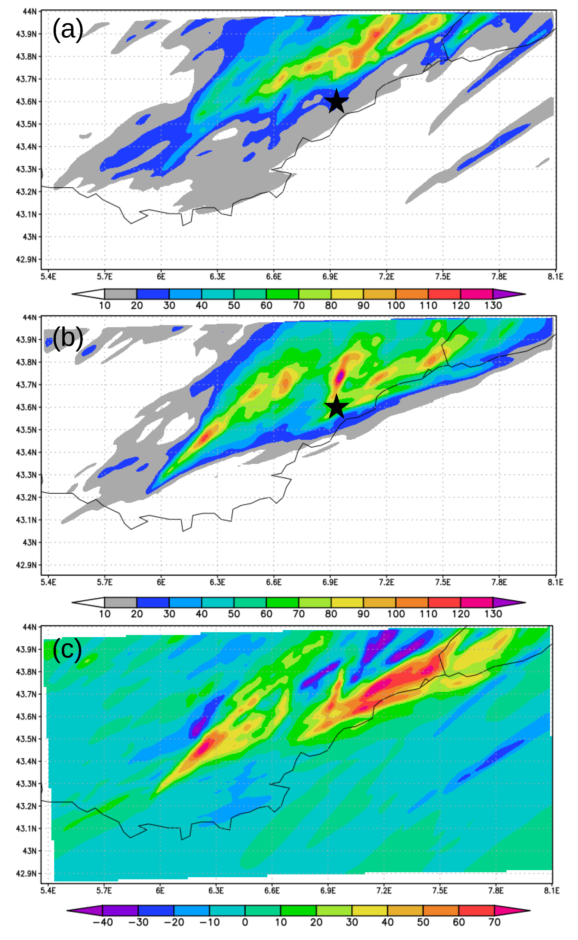
The Advanced Research core of the WRF model, Version 3.8.1, was adopted in this study. The WRF model is a fully compressible non-hydrostatic, primitive-equation model with multiple nesting capabilities. A comprehensive description of the model formulation is given in [35]. Several physics options are available in WRF for the parameterization of unresolved sub-grid phenomena; in the present work we adopted a model configuration quite similar to that used operationally at the University of Genoa and described in [27,33,36]. We defined three two-way nested computational domains in a Lambert Conic Conformal projection, covering western and central Europe with horizontal resolution of 10 km, the central part of the northern Mediterranean basin with horizontal resolution of 3.3 km and the Côte d’Azur region with a grid spacing of 1.1 km (Figure 6).

The number of terrain-following vertical levels adopted in this work was 35, with higher resolution close to the surface. For the short wave solar radiation the Goddard scheme [37] was selected, whereas for the long-wave radiation the Rapid Radiation Transfer Model (RRTM) scheme [38] was adopted. The Kain–Fritsch parameterization [39] was used for cumulus in the coarser resolution domain only, whereas in the higher resolution domains convective processes were explicitly resolved. Furthermore, the Mellor–Yamada–Janjic scheme [40] for the boundary layer, the Eta similarity surface layer scheme [40] and the Noah land surface model [41] were chosen. Microphysical schemes are the parameterizations responsible for computing atmospheric water vapour, cloud liquid water, cloud ice and various types of precipitation, therefore they are crucial for a correct prediction of severe rainfall events. In the present work we adopted the Milbrandt cloud microphysics scheme which, after a preliminary analysis (not shown for the sake of brevity), was found to provide most reliable results. The Milbrandt cloud microphysical scheme is a double moment scheme providing concentration number and mass evolution of six different classes of hydrometeors [42].

4. Results

The extremely limited spatio-temporal localization of the presented event contributed to a quite poor predictability. In the present section we analyse the impact of resolution and initial and boundary conditions on the capability of the model in forecasting the event described above, in order to highlight the reason why the event was largely underestimated in operational simulations. We also investigated the response of the precipitation predicted by the model to the sea surface temperature (SST) field ingested as a lower boundary conditions, which can play a crucial role in triggering the development of convective cells, as shown in [27].

In

Table 1. List of all the simulations performed in the present work corresponding to different initializations (first column) and corresponding acronyms (second column).

Simulation	Acronym
GFS	W_GFS
GFS + satellite SST	W_GFS_SST
ECMWF	W_ECM
ECMWF + satellite SST	W_ECM_SST
GFS analysis	W_GFSANL
GFS analysis + satellite SST	W_GFSANL_SST

all simulations performed in the present work, corresponding to different initializations (first column) and corresponding acronyms (second column) used in the following of the paper, are listed. In the first column, GFS—Global Forecast System and ECMWF—European Center Medium Weather Forecast, refer to the global model utilized for WRF initialization. The wording ’satellite SST’ is used when high resolution satellite SST replaced coarser global models SST. Finally, analysis means that WRF was initialized adopting as boundary conditions the analyses of different GFS model runs.

In Figure 7 the effect of the model resolution, and in particular the need to explicitly describe convection, is highlighted. Here the simulated precipitation, accumulated between 17 UTC and 23 UTC of 3 October 2015, over the three domains, is represented. For this first set of simulations, WRF initialization was provided by GFS operational run (0.5${}^{\circ }$ × 0.5${}^{\circ }$ resolution); 00 UTC analysis of 3 October 2015, and three-hourly GFS model forecast fields were respectively imposed as initial and boundary conditions [43].

When convection was explicitly resolved, the Figure 7b,c, precipitation forecast considerably increased inasmuch as the simulation was able to describe the development of the convective system responsible for the flood, although attenuated and shifted inland with respect to the actual position. Comparing the 10 km resolution to the 1.1 km resolution simulations, the precipitation peak was realistically more spatially concentrated and the amount increased by about 40%. For this reason all of the following discussion will be focused on 1.1 km resolution simulations.

4.1. Sensitivity to Initial Conditions and SST

Recent studies highlighted the effects that SST inhomogeneities can produce on Mediterranean convective storms. This fact is supported by the period of the year usually affected by severe events. Floods in the central part of the Mediterranean basin are usually observed during a relatively narrow time window ranging between late summer and mid autumn. During this period of the year, the exchange of heat and moisture between sea surface and atmosphere is maximum suggesting to pay particular attention to the role played by the SST when having to deal with intense convective system. A further simulation was therefore performed ingesting high-resolution satellite-retrieved SST data. The quite low resolution that characterizes global model does not allow to correctly represent small scale SST variations. The GFS SST field, for example, is derived from the assimilation of data obtained during the previous seven days [43]. For this set of simulations the CNR MED L4 ultra-high-resolution (UHR, corresponding to 0.01 degree) SST data were adopted. This database was obtained from infrared satellite radiometers. The observations are then interpolated through statistical methods. The data are collected by different satellites every day between 9:00 PM and 6:00 AM of the next day in order to avoid any diurnal warming contamination. Finally, the observed data were spatially and temporally merged through an optimal interpolation algorithm to create a daily 00 UTC SST field [44].

Differences between the two SST fields used (the one provided by GFS model and ultra-high resolution SST field produced by CNR) were generally moderate, but reached about 2 °C in the coastal area around Cannes, Figure 8a, probably due to land-sea interpolation issues (see also [45] about this point).

Such temperature differences were however sufficient to increase precipitation peak intensity of about 10% (Figure 8b) with respect to the case in which no substitution of SST took place. Furthermore, convective systems responsible for precipitations were shifted southward, in the direction of the coast, approaching the observed precipitation peak localization (Figure 8c). On the other hand, further precipitation peaks appeared to the right and left of the principal one possibly due to the increased atmospheric instability related to the ingestion of a higher coastal SST.

Despite the improvement reached by introducing ultra-high resolution SST, the intensity of convective system responsible for the flood was still underestimated and localized too inland and split into different secondary peaks, possibly due to inaccuracies in the initial and boundary conditions provided to WRF model by the GFS model. In [27] is shown that the ingestion of a satellite-retrieved SST initial field improved the quantitative precipitation forecast only when the description of large scale forcing was accurate enough to reasonably describe the convective initiation and development. If the large scale model missed key dynamical features, the mesoscale model turned out to be unable to correctly capture the evolution of the extreme event under investigation despite the use of a reliable high resolution SST field.

To investigate this aspect, a different global model was used to initialize WRF, in the attempt to find out the large scale features that might be responsible for the forecast deficiencies. A new set of simulations was therefore carried out initializing WRF with higher resolution fields obtained from forecast provided by the ECMWF Integrated Forecasting System model with a grid spacing of about 12.5 km.

In Figure 9a, the surface temperature difference between ECMWF-driven (W_ECM) and GFS-driven (W_GFS) simulations at 15 UTC, 3 October 2015, just before the starting of the event, is reported. W_ECM simulation presents higher temperature values just in the area affected by precipitation, resulting in higher Convective Available Potential Energy—CAPE (Figure 9b), which in turn can be, in principle, associated to enhanced convection and precipitation intensity.

The results of W_ECM simulation in terms of precipitation are presented in Figure 10a, where precipitation accumulated between 17 UTC and 23 UTC of 3 October 2015, is reported. The precipitation pattern was quite similar to those produced with GFS initialization (again, precipitation peak was attenuated and shifted inland with respect to observations), except for a considerable strengthening of the convective cell present across the Italian border.

When utilizing initial and boundary conditions provided by ECMWF model simulations, the effect of ingesting high resolution satellite-derived SST was somehow different with respect to what was observed with GFS initialization. The most remarkable result consisted in an attenuation of precipitation (Figure 10b), although, again, the precipitation pattern was shifted southward (Figure 10c).

In this case, the satellite SST field presented generally lower values with respect to SST assumed by ECMWF analysis, with the exception of a very narrow nearshore belt (Figure 11a). The reduced extension (if compared with GFS initialization) of this warmer sea area was mainly due to the higher resolution of the ECMWF model, resulting in a more accurate interpolation at the land-sea interface. However, apparently minor variations in the SST field between the W_ECM and W_ECM_SST simulations were sufficient to induce a modification of the precipitation pattern and a displacement of the maxima towards the sea (Figure 11a). The substantial differences between the SST fields provided by GFS and ECMWF models lay in the different sources of data and in the different way in which data themselves were assimilated into the two global models [46,47,48].

Summarizing, WRF simulations initialized both with GFS and ECMWF models, despite being somehow able to reproduce the cell responsible for Cannes flood in the evening of the 3 October 2015, presented some difficulties both in localizing the cell properly and in quantifying the precipitation amount precisely. The introduction of a high-resolution SST always had a positive effect in terms of localization of the precipitation patterns; this fact was probably due to the GFS and ECMWF analysis underestimation of the portion of SST field near the coast, and hence closest to the convective cell. The nearshore temperature increased with respect to inland areas results in a modification of local wind pattern (not shown) producing a southward shift of the cells in direction of the coast.

Looking at offshore areas, the CNR SST field was, on average, cooler with respect to the ECMWF SST (Figure 11b) analysis. The overall cooling of the lowest portion of atmosphere due to the introduction of a different SST fields resulted in a weakening of the moisture advection from the sea and, consequently, in a reduction of simulated precipitation, Figure 10c. The opposite situation occurred when CNR data were substituted to GFS SST analysis. In this case GFS SST was, in average, underestimated (Figure 8a) with respect to the satellite-derived field and, as a consequence, the introduction of a warmer SST resulted in a strengthening of convection and hence in an intensification of precipitation.

4.2. Sensitivity to Lateral Boundary Conditions

The last part of this analysis was devoted to evaluate the effect of large-scale boundary conditions on the simulations and, in particular, on the quantitative precipitation forecast. Starting from the same initial conditions, a new set of simulations was performed adopting as boundary conditions the analyses of different GFS model runs: namely, the 00 UTC GFS run of 3 October, 2015 provided WRF initial conditions while the analyses of the eight subsequent runs (06, 12, 18 and 00, 06, 12, 18, 00 UTC of the following days) provided boundary conditions. Although a less frequent update of lateral boundary conditions might be, in principle, detrimental to mesoscale simulations, analysis data were expected to approach more closely real atmospheric conditions with respect to forecast data, because they were obtained from the data assimilation process and hence were not subject to forecast errors introduced during the global model simulation.

In Figure 12a, 6 h cumulated precipitation simulated by the WRF model driven by GFS analysis fields is reported. Precipitation intensity further increased reaching 116 mm accumulated between 17 UTC and 23 UTC of 3 October 2015, however still being underestimated and localized too inland. So, despite the simulation improvement, acting only on boundary conditions was not sufficient to describe the event in a satisfactory way.

Trying to combine more reliable boundary conditions with best SST data available, again the ultra-high-resolution CNR SST field was introduced in place of coarser GFS SST analysis. The result of this substitution is shown in Figure 12b. A further increase of simulated precipitation was evident together with a remarkable southward shift of the convective structure responsible for the flood. This fact is highlighted in Figure 12c, where the 6 h accumulated precipitation difference between simulation initialized by GFS analysis with and without the CNR SST ingestion is reported. In this last case, the assimilation of a more reliable SST produced the highest improvement in precipitation intensity among all simulations produced so far. In particular, the adoption of more accurate boundary conditions deriving from GFS analysis and the ingestion of CNR high-resolution SST concurred to increase the simulated precipitation intensity (about 150 mm in 6 hours), approaching the observed one. Results are consistent with those previously produced when ingesting high resolution SST, underlining once again the link between the inland localization of the convective cell and the nearshore SST anomalies (Figure 8b).

In

Table 2. Simulations performed in the present paper and corresponding 6 h (17 UTC–23 UTC, 3 October 2015) precipitation maxima (mm).

Simulation	6 h Cumulated Precipitation mm
W_GFS	105.6
W_GFS_SST	115.4
W_ECM	120.4
W_ECM_SST	89.0
W_GFSANL	116.4
W_GFSANL_SST	147.8

the performed simulations together with the corresponding precipitations peaks are summarized. Although the introduction of a more accurate SST always caused an improvement in the localization of the convective cells, forecast precipitation intensity improved only when SST substitution was associated to GFS initialization. This fact, as previously discussed, is related to the opposite sign of the anomalies introduced in initial conditions when ingesting satellite SST data. In the case of initialization with ECMWF data, the ingestion of CNR SST data had a cooling effect on lower atmospheric layers, resulting in a weakening of the convection; the opposite scenario occurred in the case of GFS initialization, CNR SST data being warmer, on average, with respect to the GFS field.

To further investigate the effect of ingesting different SSTs in WRF, in Figure 13 an equivalent potential temperature cross section is reported. The cross section was taken in correspondence of the most intense convective cell (43.65${}^{\circ }$ N) at 19 UTC, 3 October 2015. Contours refer to cloud water mixing ratio (g kg${}^{-1}$). Left panels refer to cross sections obtained using global models SST, while right panels were obtained ingesting in WRF model the high-resolution SST data. The most evident aspect was the cloud water mixing ratio maxima migration in direction of the coast when CNR SST is used. Again, the importance of correctly describing surface temperature close to land-sea interface appears to be fundamental in determining convective system localization. Furthermore, in the case of W_ECM_SST (Figure 14d), the vertical extension of cloud water mixing ratio was considerably reduced, indicating a shallower convection, consistent with the introduction of a cooler SST (at least offshore and on average) with respect to the original one. These results are confirmed by Figure 14 where vertical velocity cross sections at the same time and for the same latitude are reported. In the case of W_ECM_SST simulation the vertical development of the convective cell was not sufficient to produce heavy precipitation, and the maxima of the cloud water mixing ratio were not associated to strong descending vertical velocity (Figure 14d). In the case of W_GFS_SST and W_GFSANL_SST simulations, maxima of cloud water mixing ratio corresponded to strong downward vertical velocity, indicating more severe convection resulting in an increase of total precipitation.

5. Conclusions

Floods that often affect coastal region of the central part of the Mediterranean Basin during autumn are almost always associate to small-sized, quasi-stationary mesoscale V-shaped convective systems. The extremely limited spatio-temporal localization of these kind of events contributes to a quite poor predictability of the events themselves, making their forecast very challenging.

One of these catastrophic events hit the area around Cannes during October 2015. In the present paper we have analysed the impact of resolution and initial and boundary conditions on the capability of the WRF model in forecasting the Cannes flood. Only high resolution simulations, allowing explicitly resolved convection, are able to provide accurate description of the event, if associated to reliable initial/boundary conditions. To perform an analysis of the role of the initial/boundary conditions, fields provided by different global models (GFS and ECMWF) were ingested by the WRF model. To single out the effect of boundary conditions, starting from the same initial conditions provided by GFS model, a further set of simulations were performed adopting as boundary conditions the analyses of different GFS model runs. Finally, the present study investigated the response of the precipitation predicted by the model to the SST field ingested as a lower boundary conditions. The role of SST is assessed combining previous model initializations with ultra-high-resolution CNR SST field.

Our results clearly show the ability of WRF model in forecasting very intense flood-causing precipitations in complex areas influenced by nontrivial dynamical interactions between orographycally complex lands and sea. A necessary condition to reach a good level of accuracy is the availability of accurate initial/boundary conditions coming from large-scale model/observations. If the large scale model misses key dynamical features, the mesoscale model, even if running at high resolutions, turns out to be unable to capture the details of the extreme event under investigation. This result points to the importance of suitable downscaling strategies starting from large scale ensemble predictions (as, e.g., the ECMWF Ensemble Prediction System (EPS) [49]) and the Global Ensemble Forecast System (GEFS) [50,51]). The most accurate members of the ensemble forecasts in relation to the large-scale features, are expected to generate accurate small-scale features once they are ingested into high-resolution mesoscale models as initial/boundary conditions. However, in case the lack of predictability at the mesoscale is related to purely convective instability rather than instability associated to synoptic scale features, to address which global ensemble forecasts are designed [52], a simple downscaling strategy might just provide a zoom of synoptic instabilites, while convective instabilities would remain substantially unexplored. Therefore, a “poor man’s” ensemble of several independent deterministic high-resolution models can provide added value allowing for an operationally low-cost probabilistic approach [53]. Whether or not a dynamical downscaling of the 50 members of the ECMWF EPS will produce accurate probabilistic prediction of mesoscale extreme events as the one we have considered here is a subject we are currently investigating.

References

1. Dayan, U.; Nissen, K.; Ulbrich, U. Review Article: Atmospheric conditions inducing extreme precipitation over the eastern and western Mediterranean. Nat. Hazards Earth Syst. Sci. 2015, 15, 2525–2544. [Google Scholar] [CrossRef] [Green Version]
2. Pontrelli, M.D.; Bryan, G.H.; Fritsch, J.M.; Estrela, M.J. The Madison County, Virginia, flash flood of 27 June 1995. Weather Forecast. 1999, 14, 384–404. [Google Scholar] [CrossRef]
3. Lin, Y.L.; Chiao, S.; Wang, T.A.; Kaplan, M.L.; Weglarz, R.P. Some common ingredients for heavy orographic rainfall. Weather Forecast. 2001, 16, 633–660. [Google Scholar] [CrossRef]
4. Miglietta, M.M.; Rotunno, R. Application of theory to observed cases of orographically forced convective rainfall. Mon. Weather Rev. 2012, 140, 3039–3053. [Google Scholar] [CrossRef]
5. McCann, D.W. The enhanced-V: A satellite observable severe storm signature. Mon. Weather Rev. 1983, 111, 887–894. [Google Scholar] [CrossRef] [Green Version]
6. Davolio, S.; Mastrangelo, D.; Miglietta, M.M.; Drofa, O.; Buzzi, A.; Malguzzi, P. High resolution simulations of a flash flood near Venice. Nat. Hazard Earth Syst. Sci. 2009, 9, 1671–1678. [Google Scholar] [CrossRef]
7. Buzzi, A.; Davolio, S.; Malguzzi, P.; Drofa, O.; Mastrangelo, D. Heavy rainfall episodes over Liguria of autumn 2011: Numerical forecasting experiment. Nat. Hazards Earth Syst. Sci. Discuss. 2013, 1, 7093–7135. [Google Scholar] [CrossRef]
8. Fiori, E.; Commellas, A.; Molini, L.; Rebora, N.; Siccardi, F.; Gochis, D.J.; Tanelli, S.; Parodi, A. Analysis and hindcast simulation of an extreme rainfall event in the Mediterranean area: The Genoa 2011 case. Atmos. Res. 2014, 138, 13–29. [Google Scholar] [CrossRef] [Green Version]
9. Davolio, S.; Volonté, A.; Manzato, A.; Pucillo, A.; Cicogna, A.; Ferrario, M.E. Mechanisms producing different precipitation patterns over north-eastern Italy: Insights from HyMeX-SOP1 and previous events. Q. J. R. Meteorol. Soc. 2016, 142, 188–205. [Google Scholar] [CrossRef] [Green Version]
10. Ricard, D.; Ducrocq, V.; Auger, V. A climatology of the mesoscale environment associated with heavily precipitating events over a Northwestern Mediterranean area. J. Appl. Meteorol. Climatol. 2012, 51, 468–488. [Google Scholar] [CrossRef]
11. Drobinski, P.; Ducrocq, V.; Alpert, P.; Anagnostou, E.; Beranger, K.; Borga, M.; Braud, I.; Chanzy, A.; Davolio, S.; Delrieu, G.; et al. HyMeX: A 10-year multidisciplinary program on the Mediterranean water cycle. Bull. Am. Meteorol. Soc. 2014, 95, 1063–1082. [Google Scholar] [CrossRef]
12. Booth, J.F.; Thompson, L.; Patoux, J.; Kelly, K.A. Sensitivity of Midlatitude Storm Intensification to Perturbations in the Sea Surface Temperature near the Gulf Stream. Mon. Weather Rev. 2012, 140, 1241–1256. [Google Scholar] [CrossRef]
13. Katsafados, P.; Mavromatidis, E.; Papadopoulos, A.; Pytharoulis, I. Numerical simulation of a deep Mediterranean storm and its sensitivity on sea surface temperature. Nat. Hazards Earth Syst. Sci. 2011, 11, 1233–1246. [Google Scholar] [CrossRef]
14. Ludwig, P.; Pinto, J.G.; Reyers, M.; Gray, S.L. The role of anomalous SST and surface fluxes over the southeastern North Atlantic in the explosive development of windstorm Xynthia. Q. J. R. Meteorol. Soc. 2014, 140, 1729–1741. [Google Scholar] [CrossRef] [Green Version]
15. Meredith, E.P.; Semenov, V.A.; Maraun, D.; Park, W.; Chernokulsky, A.V. Crucial role of Black Sea warming in amplifying the 2012 Krymsk precipitation extreme. Nat. Geosci. 2015, 8, 615–619. [Google Scholar] [CrossRef]
16. Iizuka, S.; Nakamura, H. Sensitivity of Midlatitude Heavy Precipitation to SST: A Case Study in the Sea of Japan Area on 9 August 2013. J. Geophys. Res. Atmos. 2019, 124, 4365–4381. [Google Scholar] [CrossRef] [Green Version]
17. Yamamoto, M. Ensemble simulations of the influence of regionally warm sea surface on moisture and rainfall in Tsushima Strait during August 2013. Atmos. Res. 2020, 238, 104876. [Google Scholar] [CrossRef]
18. Ducrocq, V.; Nuissier, O.; Ricard, D.; Lebeaupin, C.; Thouvenin, T. A numerical study of three catastrophic precipitating events over southern France. II: Mesoscale triggering and stationarity factors. Q. J. R. Meteorol. Soc. 2008, 134, 131–145. [Google Scholar] [CrossRef]
19. Nuissier, O.; Ducrocq, V.; Ricard, D.; Lebeaupin, C.; Anquetin, S. A numerical study of three catastrophic precipitating events over southern France, I: Numerical framework and synoptic ingredients. Q. J. R. Meteorol. Soc. 2008, 134, 111–130. [Google Scholar] [CrossRef]
20. Silvestro, F.; Gabellani, S.; Giannoni, F.; Parodi, A.; Rebora, N.; Rudari, R.; Siccardi, F. A hydrological analysis of the 4 November 2011 event in Genoa. Nat. Hazards Earth Syst. Sci. 2012, 12, 2743–2752. [Google Scholar] [CrossRef]
21. Silvestro, F.; Rebora, N.; Giannoni, F.; Cavallo, A.; Ferraris, L. The flash flood of the Bisagno Creek on 9th October 2014: An “unfortunate” combination of spatial and temporal scales. J. Hydrol. 2016, 541, 50–62. [Google Scholar] [CrossRef] [Green Version]
22. Lagasio, M.; Parodi, A.; Procopio, R.; Rachidi, F.; Fiori, E. Lightning Potential Index performances in multimicrophysical cloud-resolving simulations of a back-building mesoscale convective system: The Genoa 2014 event. J. Geophys. Res. Atmos. 2017, 122, 4238–4257. [Google Scholar] [CrossRef]
23. Pastor, F.; Estrela, M.J.; Peñarrocha, D.; Millán, M.M. Torrential Rains on the Spanish Mediterranean Coast: Modeling the Effects of the Sea Surface Temperature. J. Appl. Meteorol. 2001, 40, 1180–1195. [Google Scholar] [CrossRef]
24. Lebeaupin, C.; Ducrocq, V.; Giordani, H. Sensitivity of torrential rain events to the sea surface temperature based on high-resolution numerical forecasts. J. Geophys. Res. Atmos. 2006, 111, D12. [Google Scholar] [CrossRef] [Green Version]
25. Berthou, S.; Mailler, S.; Drobinski, P.; Arsouze, T.; Bastin, S.; Beranger, K.; Lebeaupin-Brossier, C. Sensitivity of an intense rain event between atmosphere-only and atmosphere-ocean regional coupled models: 19 September 1996. Q. J. R. Meteorol. Soc. 2015, 141, 258–271. [Google Scholar] [CrossRef]
26. Pastor, F.; Valiente, J.A.; Estrela, M.J. Sea surface temperature and torrential rains in the Valencia region: Modelling the role of recharge areas. Nat. Hazards Earth Syst. Sci. 2015, 15, 1677–1693. [Google Scholar] [CrossRef] [Green Version]
27. Cassola, F.; Ferrari, F.; Mazzino, A.; Miglietta, M.M. The role of the sea on the flash floods events over Liguria (northwestern Italy). Geophys. Res. Lett. 2016, 43, 3534–3542. [Google Scholar] [CrossRef]
28. Meroni, A.N.; Parodi, A.; Pasquero, C. Role of SST Patterns on Surface Wind Modulation of a Heavy Midlatitude Precipitation Event. J. Geophys. Res. Atmos. 2018, 123, 9081–9096. [Google Scholar] [CrossRef]
29. Stocchi, P.; Davolio, S. Intense air-sea exchanges and heavy orographic precipitation over Italy: The role of Adriatic sea surface temperature uncertainty. Atmos. Res. 2017, 196, 62–82. [Google Scholar] [CrossRef]
30. Miglietta, M.M.; Mazon, J.; Motola, V.; Pasini, A. Effect of a positive Sea Surface Temperature anomaly on a Mediterranean tornadic supercell. Sci. Rep. 2017, 7, 12828. [Google Scholar] [CrossRef] [Green Version]
31. Miglietta, M.M.; Moscatello, A.; Conte, D.; Mannarini, G.; Lacorata, G.; Rotunno, R. Numerical analysis of a Mediterranean ‘hurricane’ over south-eastern Italy: Sensitivity experiments to sea surface temperature. Atmos. Res. 2011, 101, 412–426. [Google Scholar] [CrossRef]
32. Ricchi, A.; Miglietta, M.M.; Barbariol, F.; Benetazzo, A.; Bergamasco, A.; Bonaldo, D.; Cassardo, C.; Falcieri, F.M.; Modugno, G.; Russo, A.; et al. Sensitivity of a Mediterranean Tropical-Like Cyclone to Different Model Configurations and Coupling Strategies. Atmosphere 2017, 8, 92. [Google Scholar] [CrossRef] [Green Version]
33. Cassola, F.; Ferrari, F.; Mazzino, A. Numerical simulations of Mediterranean heavy precipitation events with the WRF model: A verification exercise using different approaches. Atmos. Res. 2015, 164–165, 3–18. [Google Scholar] [CrossRef]
34. Goulet, L. The Catastrophic Event of October 3rd 2015 in Cannes. Eur. Forecast. 2016, 21, 12–22. [Google Scholar]
35. Skamarock, W.C.; Klemp, J.B.; Dudhia, J.; Gil, D.O.; Barker, D.M.; Duda, M.G.; Huang, X.Y.; Wang, W.; Powers, J.G. A Description of the Advanced Research WRF. Version 3; Technical Report. National Center for Atmospheric Research, 2008. Available online: https://opensky.ucar.edu/islandora/object/technotes:500 (accessed on 30 April 2020).
36. Bove, M.C.; Brotto, P.; Cassola, F.; Cuccia, E.; Massabò, D.; Mazzino, A.; Piazzalunga, A.; Prati, P. An integrated PM2.5 source apportionment study: Positive Matrix Factorization vs. the chemical transport model CAMx. Atmos. Environ. 2014, 94, 274–286. [Google Scholar] [CrossRef]
37. Chou, M.D.; Suarez, M.J. An Efficient Thermal Infrared Radiation Parameterization for Use In General Circulation Models. Technical Report; NASA/Goddard Space Flight Center, 1994. Available online: https://ntrs.nasa.gov/search.jsp?R=19950009331 (accessed on 30 April 2020).
38. Mlawer, E.J.; Taubman, S.J.; Brown, P.D.; Iacono, M.J.; Clough, S.A. Radiative transfer for inhomogeneous atmosphere: RRTM, a validated correlated k-model for the long-wave. J. Geophys. Res. 1997, 102, 663–682. [Google Scholar] [CrossRef] [Green Version]
39. Kain, J.S. The Kain-Fritsch convective parameterization: An update. J. Appl. Meteorol. 2004, 43, 170–181. [Google Scholar] [CrossRef] [Green Version]
40. Janjic, Z.I. Non Singular Implementation of the Mellor-Yamada Level 2.5 Scheme in the NCEP Meso Model. Technical Report 437. NOAA Science Center, 2002. Available online: https://pdfs.semanticscholar.org/08a1/48851340d682d16aab9257889be824eb8812.pdf?$_$ga=2.82424336.78943031.1591095320-1205471210.1591095320 (accessed on 30 April 2020).
41. Chen, F.; Dudhia, J. Coupling an advanced land-surface/hydrology model with the Penn state/NCAR MM5 modeling system. Part I: Model description and implementation. Mon. Weather Rev. 2001, 12, 569–585. [Google Scholar] [CrossRef] [Green Version]
42. Milbrandt, J.A.; Yau, M.K. A Multimoment Bulk Microphysics Parameterization. Part II: A Proposed Three-Moment Closure and Scheme Description. J. Atmos. Sci. 2005, 62, 3065–3081. [Google Scholar] [CrossRef]
43. Environmental Modeling Center. The GFS Atmospheric Model; NCEP Office Note 442; National Oceanic and Atmospheric Administration, 2003. Available online: http://nws.noaa.gov/ost/climate/STIP/AGFS$_$DOC$_$1103.pdf (accessed on 30 April 2020).
44. Buongiorno-Nardelli, B.; Tronconi, C.; Pisano, A.; Santoleri, R. High and Ultra-High resolution processing of satellite Sea Surface Temperature data over Southern European Seas in the framework of MyOcean project. Remote Sens. Environ. 2013, 129, 1–16. [Google Scholar] [CrossRef]
45. Ricchi, A.; Miglietta, M.M.; Falco, P.P.; Benetazzo, A.; Bonaldo, D.; Bergamasco, A.; Sclavo, M.; Carniel, S. On the use of a coupled ocean–atmosphere–wave model during an extreme cold air outbreak over the Adriatic Sea. Atmos. Res. 2016, 172–173, 48–65. [Google Scholar] [CrossRef]
46. Bonavita, M.; Holm, E.; Isaksen, L.; Fisher, M. The evolution of the ECMWF hybrid data assimilation system. Q. J. R. Meteorol.Soc. 2016, 142, 287–303. [Google Scholar] [CrossRef]
47. Szunyogh, I.; Kostelich, J.E.; Gyarmati, G.; Kalnay, E.; Hunt, B.R.; Ott, E.; Satterfield, E.; Yorke, J.A. A local ensemble transform Kalman filter data assimilation system for the NCEP global model. Tellus A Dyn. Meteorol. Oceanogr. 2008, 60, 113–130. [Google Scholar] [CrossRef]
48. Wang, X.; Parrish, D.; Kleist, D.; Whitaker, J. GSI 3DVar-Based Ensemble–Variational Hybrid Data Assimilation for NCEP Global Forecast System: Single-Resolution Experiments. Mon. Weather Rev. 2013, 141, 4098–4117. [Google Scholar] [CrossRef]
49. Palmer, T. The ECMWF ensemble prediction system: Looking back more than 25 years and projecting forward 25 years. Q. J. R. Meteorol. Soc. 2019, 145, 12–24. [Google Scholar] [CrossRef] [Green Version]
50. Wei, M.; Toth, Z.; Wobus, R.; Zhu, Y.; Bishop, C.H.; Wang, X. Ensemble Transform Kalman Filter-based ensemble perturbations in an operational global prediction system at NCEP. Tellus A Dyn. Meteorol. Oceanogr. 2006, 58, 28–44. [Google Scholar] [CrossRef]
51. Wei, M.; Toth, Z.; Wobus, R.; Zhu, Y. Initial perturbations based on the ensemble transform (ET) technique in the NCEP global operational forecast system. Tellus A Dyn. Meteorol. Oceanogr. 2008, 60, 62–79. [Google Scholar] [CrossRef] [Green Version]
52. Hohenegger, C.; Schaer, C. Atmospheric predictability at synoptic versus cloud-resolving scales. Bull. Am. Meteorol. Soc. 2007, 88, 1783–1793. [Google Scholar] [CrossRef]
53. Corazza, M.; Sacchetti, D.; Antonelli, M.; Drofa, O. The ARPAL operational high resolution Poor Man’s Ensemble, description and validation. Atmos. Res. 2018, 203, 1–15. [Google Scholar] [CrossRef]
Figure 1. Synoptic situation over Europe at 00 UTC, 3 October 2015. Panel (a): UK Met Office analysis (from http://www.wetterzentrale.de/). Panel (b): 500 hPa geopotential height (geopotential decameter-gpdm , shaded contours) and mean sea level pressure (hPa, white contours) at 00 UTC, 3 October 2015. CFSR reanalysis from http://www.wetterzentrale.de/.
Atmosphere 11 00592 g001
Figure 2. 10 m, panel (a), and 850 hPa, panel (b), wind fields (magnitude and vector, m s 1 ), referred to 00 UTC, 3 October 2015, produced by the Global Forecast System model.
Atmosphere 11 00592 g002
Figure 3. Radar image of precipitation that hit Provence-Alpes-Côte d’Azur region at (a) 17.00, (b) 19.00, (c), 20.00 and (d), 20.45 local time. Colour scale ranges from light blue for light rain to white for heavy rain. National Weather Service (Meteo France).
Atmosphere 11 00592 g003
Figure 4. Hourly rainfall in Cannes (mm) from 00 UTC, 1 October 2015 and 12 UTC, 4 October 2015. National Weather Service (Meteo France).
Atmosphere 11 00592 g004
Figure 5. Extension of the innermost simulation domain adopted in this study and of the area affected by severe convection (left) and rain accumulations (mm) provided by the ANTILOPE analysis between 17 UTC and 20 UTC, 3 October 2015 (right). ANTILOPE product is based on both radar data and measurements from the rain gauge network (Meteo France).
Atmosphere 11 00592 g005
Figure 6. Topography (m) of the outermost Weather Research and Forecasting (WRF) computational domain (10 km resolution) and location of the two nested domains over western Alps and central Mediterranean basin (larger box, 3.3 km resolution) and the Côte d’Azur region (smaller box, 1.1 km resolution).
Atmosphere 11 00592 g006
Figure 7. Cumulated precipitation (mm) over 6 h predicted over Provence-Alpes-Côte d’Azur area by the WRF model at different resolutions: 10 km , (a), 3.3 km, (b), and 1.1 km, (c). Simulations are initialized at 00 UTC of 3 October 2015 using GFS fields and the accumulation period is 17 UTC–23 UTC. Black star identifies observed precipitation peak localization.
Atmosphere 11 00592 g007
Figure 8. Panel (a): Sea surface temperature (SST) difference (°C) between satellite-derived and GFS analyses at 00 UTC, 3 October 2015. Panel (b): 6 h simulated precipitation (mm) provided by W_GFS_SST simulation. Panel (c): 6 h cumulated precipitation difference (mm) between W_GFS and W_GFS_SST simulations. Accumulation period is 17 UTC–23 UTC, 3 October 2015. Black star identifies observed precipitation peak localization.
Atmosphere 11 00592 g008
Figure 9. Panel (a): Surface temperature difference (°C) between ECMWF-driven (W_ECM) simulation and GFS-driven (W_GFS) simulations, at 15 UTC, 3 October 2015. Panel (b): surface Convective Available Potential Energy (CAPE) difference (J kg 1 ) between W_ECM simulation and W_GFS simulations, at 15 UTC, 3 October 2015.
Atmosphere 11 00592 g009
Figure 10. Panel (a): The 6 h simulated precipitation (mm) provided by W_ECM simulation. Panel (b): the 6 h simulated precipitation (mm) provided by W_ECM_SST. Panel (c): 6 h cumulated precipitation difference (mm) between W_ECM and W_ECM_SST simulations. Accumulation period is 17 UTC–23 UTC, 3 October 2015. Black star identifies observed precipitation peak localization.
Atmosphere 11 00592 g010aAtmosphere 11 00592 g010b
Figure 11. Panel (a): SST difference (°C) between satellite-derived and ECMWF analyses at 00 UTC, 3 October 2015. Panel (b): 17 UTC surface temperature difference (shade contour) between 3.3 km resolution W_ECM_SST and W_ECM simulations and W_ECM_SST 10 m wind field (vector m s 1 ).
Atmosphere 11 00592 g011
Figure 12. Panel (a): the 6 h simulated precipitation (mm) provided by W_GFSANL. Panel (b): 6 h simulated precipitation provided by W_GFSANL_SST. Panel (c): 6 h cumulated precipitation difference (mm) between W_GFSANL and W_GFSANL_SST. Accumulation period is 17 UTC–23 UTC, 3 October 2015. Black star identifies observed precipitation peak localization.
Atmosphere 11 00592 g012
Figure 13. Equivalent potential temperature (K, shaded contours) and cloud water mixing ratio (g kg 1 , line contours) cross sections, taken at 43.65 N, and shown in panel (a), at 19 UTC, 3 October 2015 for (b) W_GFS, (c) W_GFS_SST, (d) W_ECM, (e) W_ECM_SST, (f) W_GFSANL and (g) W_GFSANL_SST simulations.
Atmosphere 11 00592 g013aAtmosphere 11 00592 g013b
Figure 14. Vertical velocity (Pa s 1 , shaded contours) and cloud water mixing ratio (g kg 1 , line contours) cross sections, taken at 43.65 N, and shown in panel (a), at 19 UTC, 3 October 2015 for (b) W_GFS, (c) W_GFS_SST, (d) W_ECM, (e) W_ECM_SST, (f) W_GFSANL and (g) W_GFSANL_SST simulations.
Atmosphere 11 00592 g014aAtmosphere 11 00592 g014b