Abstract
The ionospheric response to a geomagnetic storm is a geophysical process. Although strong geomagnetic storms input more energy into the Earth’s upper atmosphere, the ionospheric response often does not reflect the same level of variation as the geomagnetic storm, and the response may be weak during a very strong storm. However, the estimated ionospheric response to geomagnetic activity also varies with extraction method. Here, two different methods—the spectral whitening method (SWM) and the monthly median method (MMM)—are used to verify whether the apparent weak ionospheric response is an artifact of the processing method. The weak ionospheric response is found with both methods, which suggests it is a real ionospheric phenomenon. The statistical characteristics of the regional and global ionospheric weak response to a super geomagnetic storm (SGS) and to an SGS with a preceding storm event (SGS-PRE) are investigated and compared. The results show that the regional ionospheric weak response to an SGS is more prevalent at middle latitudes than those at low and high latitudes. The global ionospheric weak response occurs more frequently under high solar activity and has a strong correlation with SGS-PRE, which suggests that the effect of a storm on the ionosphere can be influenced by its preconditioning, especially when there is an earlier storm and the time interval between the two storms is short. In fact, an ionospheric long-lasting disturbance may be an important reason for the ionospheric weak response caused by the SGS-PRE.
1. Introduction
The ionospheric response to geomagnetic activity is complicated and varies considerably with the phase of the geomagnetic storm [1,2,3,4,5,6]. During different storms, the energy and momentum of the solar wind plasma and the interplanetary magnetic field (IMF) are usually different. As a result, their effect on the thermosphere–ionosphere (IT) system will be significantly different. Furthermore, the dynamical, chemical, and electrodynamical processes of the IT system will usually display nonlinear interactions over a range of temporal and spatial scales. In fact, the ionosphere is not always very sensitive to geomagnetic activity, and the ionospheric weak response sometimes appears during a very strong geomagnetic storm, which is a puzzle to understand ionospheric behavior. However, the ionospheric response to a geomagnetic storm has not been well defined; in other words, the ionospheric response derived by different methods usually varies greatly, which may affect the research of weak ionospheric response to geomagnetic activity. The monthly median method (MMM) is the most commonly used approach to identify ionospheric disturbances, which is frequently used but may not be the best to separate the background and disturbance among all the median/mean methods with different window widths. A specific window width decided by the investigated issue can usually lead to better results than a fixed width of one month; however, it means that the researchers have to find a suitable width case by case due to clear and simple physical meaning, which has been used for a long time [7,8]. MMM is generally effective in obtaining the smooth and periodic ionospheric background. However, this traditional method has disadvantages. Radicella et al. [9] found that the ionospheric background is not always obtained by MMM, and Kouris et al. [10] proved that the diurnal variation of the background derived by MMM does not represent real ionospheric features. Mednikova et al. [11] found that artificial deviations (induced by MMM) in monthly medians can appear at the beginning and end of a month, which are caused by a jump from one month to another. This is particularly evident during equinoctial periods when the thermosphere is rapidly changing from winter to summer conditions. To solve these problems, many researchers have used plausible approaches to construct new measures of ionospheric disturbance [7,11,12,13], and some have used the newly defined disturbance to explore the morphology of ionospheric behavior under specific geomagnetic conditions [14,15,16,17]. The spectral whitening method (SWM) is first introduced by Wang et al. [7] and proved to be more effective in extracting geomagnetic activity from ionospheric observations [18,19], which is also very suitable to study some special ionospheric disturbance, such as strong ionospheric disturbance during geomagnetic quiet period [20]. In this study, in order to overcome the difficult of validating the real weak ionospheric response, besides the traditional MMM, the SWM are also used to verify whether the apparent weak ionospheric response to super geomagnetic storms is an artifact of the processing method or a real and common ionospheric phenomenon.
This paper is organized as follow. The data and methodology used in our statistical analysis are described in Section 2. Section 3.1 exhibits two typical events of weak ionospheric response to super geomagnetic storms. Section 3.2 define the weak ionospheric response and search the weak ionospheric response with respect to latitude and season. The global weak ionospheric response depend on different phase of solar cycle is studied in the Section 3.3. We summarize the main conclusions in Section 4.
2. Data and Methodology
2.1. Data
The data used in our analysis cover a wide geographic area, from high to low latitudes in both hemispheres. The foF2 is an important and widely used observation that has been used to explore F2-region physics for many years. However, it has the major drawback that data are often missing, sometimes for up to several months, and even several years at some stations. We therefore selected 27 ionosonde stations from the global network of 122 stations (Table 1). These are located between geographic latitudes 67.4° and −67.6° and were selected because (1) they are as widely distributed as possible, (2) the observations of foF2 from each station cover at least 30 years, and (3) their percentage of missing data is as low as possible. The common period covered by the data from all stations is from 1959 to 1990, and the temporal resolution of the data is 1 h.

Table 1.
List of ionosonde stations.
2.2. Algorithms: SWM and MMM
The main method used in this paper is the SWM, for a time series g (t), the specific algorithm of the SWM is
where is the final result of the SWM, the upper envelope of the power spectrum of and is the value that occurs most often in the dataset of .
In this paper, is foF2 and the result is ΔfoF2. The relative deviation is then defined as δfoF2 = ΔfoF2/(foF2 − ΔfoF2). The δfoF2 is the final result used to evaluate the ionospheric disturbance caused by geomagnetic activity. Similarly, a traditional monthly median method (MMM) is applied as a comparison method to obtain the corresponding δfoF2. Therefore, δfoF2-SWM and δfoF2-MMM denote the disturbance derived by SWM and MMM, respectively.
3. Results and Analysis
3.1. Single Weak Event
As shown in the upper panel of Figure 1, a strong geomagnetic storm started at 1800 UT on 5 May 1988 (shaded area in period II). The value of the geomagnetic Dst index (black line) then rapidly decreased and reached its minimum value (−160 nT) at 1000 UT the next day. Finally, it recovered to quiet time level after 10 May. During the corresponding period, the geomagnetic AE index also increased to 1334 nT. Before the geomagnetic storm (period I in Figure 1), the value of Dst remained around zero for more than a week, and the AE index was also generally at a quiet level. During this period, δfoF2 for the 27 ionosondes did not indicate any intense ionospheric disturbance. When entering period II, the ionospheric disturbances detected by most of the ionosondes are very strong, because δfoF2 rise above 0.8 for a dozen hours (lower panel of Figure 1). However, the goal of this paper is not to prove that the ionospheric disturbance derived by SWM can respond to the geomagnetic activity effectively, as this has already been verified [7,18,20]. In order to prove that the weak ionospheric response to an intense geomagnetic activity is a real geophysical phenomenon, not an artifact of the algorithm, MMM will be used as a comparison method for a weak ionospheric response event during a stronger SGS. As shown in Figure 2, another geomagnetic storm started at 1000 UT on 23 November 1982, and reached its minimum value (−197 nT) at 1700 UT the next day, and the geomagnetic AE index reached 1500 nT. Obviously, this geomagnetic storm event was more intense than the previous one, but the δfoF2 for this period at most ionosondes did not show a strong ionospheric disturbance (<0.6). The two events are compared—the first (Figure 1) with an isolated storm, and the second (Figure 2) with a preceding storm, and it can be seen that their ionospheric responses were very different, especially during period I. In the 1988 event, geomagnetic activity was very quiet in period I, and the corresponding ionospheric state was also very quiet. However, in the 1982 event, there was a geomagnetic storm in period I (as indicated by the Dst index), in which ionospheric disturbance was observed.
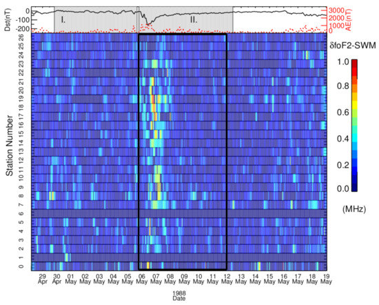
Figure 1.
Temporal variation in geomagnetic indices Dst, AE (upper panel), and δfoF2-SWM (color blocks in the lower panel) for 27 ionosondes during the period 29 April to 18 May 1988.
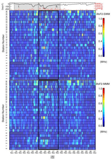
Figure 2.
Temporal variation in Dst, AE (top panel), δfoF2-SWM (color blocks in middle panel), and δfoF2-MMM (bottom panel) from 17 November to 7 December 1982.
To investigate whether this difference resulted from the algorithm, we compare the SWM results with those from the MMM. As shown in the bottom panel of Figure 2, the δfoF2 derived by MMM displays small ionospheric disturbances in most ionosondes during period I, and the geomagnetic storm is not very strong (Dst ≈ −100 nT) in this period. When the stronger geomagnetic storm occurs in period II (Dst ≈ −200 nT), the ionospheric disturbances are no stronger than during period I in most ionosondes. Further comparison of the ionospheric disturbances in Figure 1 and Figure 2 shows that the ionospheric disturbance of period II is weaker in 1982, although the geomagnetic storm of period II in 1982 is obviously stronger than that in 1988. The ionospheric disturbance of 1982 responds weakly to the second strong geomagnetic storm, and when the first smaller storm is over, the small ionospheric disturbance persists during almost the whole of period II. Even after period II, the obvious small ionospheric disturbances can still be found in the 1982 event. Clearly, long-lasting ionospheric disturbances are observed during the period 22 November to 4 December 1982. Although the method has been changed from SWM to MMM, a weak ionospheric response to an intense geomagnetic storm is still observed in period II. This suggests that this phenomenon is not an artifact of the method but might reflect the different geomagnetic conditions in period I during 1982 and 1988.
In fact, the aim of the choice of the two examples in 1982 and 1988 is to verify that the weak ionospheric response to super strong geomagnetic activity is real and not very incidental geophysical phenomenon. It seems that this finding of phenomenon is method independent: both MMM and SWM can identify this kind of phenomenon. Furthermore, comparing with the case of 1988, the ionospheric response is weaker but the geomagnetic activity is stronger in the case of 1982, which can be considered as a much weaker ionospheric response.
3.2. Regional Results and Analysis
No research has yet offered direct or powerful statistical proof that larger ionospheric disturbances appear for a stronger geomagnetic storm. The reason is that the effect of a geomagnetic storm on the ionosphere includes multiple factors, such as the variation in chemical reactions, the effect of the disturbance dynamo electric field, and the enhancement of energy inputs (such as joule heating and particle deposition) into the high latitudes [21,22,23]. These factors mean that the ionospheric response to a geomagnetic storm is complicated. Consequently, even in a very strong geomagnetic storm, the ionosphere may show a weak response in many regions.
To identify events that can truly reflect the weak ionospheric response to geomagnetic storms, the chosen geomagnetic storm events should be as strong as possible. The geomagnetic storm can be classified according to the peak Dst. [24] refers that the storm while −250 nT ≤ peak Dst ≤ −100 nT is defined as intense storm, and that while peak Dst ≤ −250 nT is defined as very intense one. In the study, in order to obtain enough and standard samples of SGS, the storm with peak Dst ≤ −200 nT is defined the event of SGS. A total number of 33 SGS events have been selected from 1959 to 1990. The response of the ionosphere is defined by the following two important parameters: the maximum value of δfoF2 (MVA) and the average value of δfoF2 (AVA) during a super storm. For a weak ionospheric response, the value of MVA should be in a reasonable range during SGS events, so this does not mean a smaller value is necessarily better. Mikhailov et al. [11] found that ionospheric disturbance (|δfoF2| > 0.2) often appears in geomagnetic quiet time. For SGS events (Dst < −200 nT), if the MVA is less than 0.2 during the storm event, it is difficult to determine whether the ionospheric disturbance is caused by the strong storm. Therefore, we select cases with MVA greater than 0.2. On the other hand, a stronger geomagnetic storm inputs more energy into the Earth’s upper atmosphere. Therefore, if we assume that the relationship between the ionospheric normal response and the geomagnetic storm is linear, the value of the weak response should be smaller than the value calculated by the linear relation.
Based on these ideas, we select six stations from high to low latitudes in the northern and southern hemispheres, and scatterplots of DstM (the minimum of Dst) against MVA during a geomagnetic storm (Dst < −100 nT) are shown in Figure 3. The linear relation varies greatly among different stations. The Pearson correlation coefficient (CC) between DstM and MVA ranged from −0.132 to −0.261, which implies very weak linear relationship between ionospheric response and geomagnetic activity. The events of very weak ionospheric response during strong geomagnetic storms can be identified in Figure 3. When DstM value reaches −200 nT, the corresponds δfoF2 value varies from 0.73 to 1.46 (seen the blue square). The value of blue square is calculated using the linear fit (red lines), while DstM equal to −200 nT. If the ionospheric response (MAV) is less than the value of blue square, this means that it is an ionospheric weak response event during the strong storm (DstM ≤ −200 nT). As shown in the Figure 3, the value of blue square is different in different station, which is ranged from 0.73 to 1.46. To correctly obtain the weak response events from all stations, we define the maximum value of |δfoF2| as 0.6. The shaded areas in Figure 3 correspond to the δfoF2 values 0.2 to 0.6, and the green dots are the selected weak response events; the value of their ionospheric response is far smaller than that given by the linear relation.
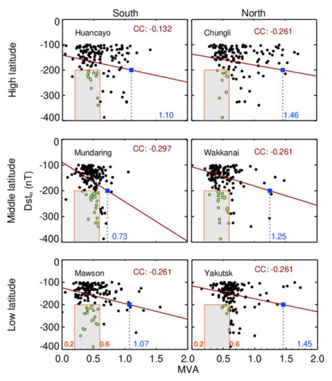
Figure 3.
Scatterplots between the minimum of Dst (DstM) and the corresponding max value of (MVA) during all geomagnetic storm events (Dst < ‒100 nT), for six selected stations from high to low latitudes in the Northern and Southern hemispheres. The shaded area is the region chosen for weak response events. The blue square is the MVA calculated using the linear fit (red lines) with a Dst of ‒200 nT. The CC is the Pearson correlation coefficient between DstM and MVA.
The weak response of the ionosphere is defined as having MVR greater than 0.2 but less than 0.6 during the period of a storm. Based on this definition, the weak ionospheric response events for 27 ionosondes are identified through the two methods (MMM and SWM) as shown in Figure 4. The weak response events (white bars in Figure 4) occur more frequently in middle latitudes than in the high and low latitudes in both hemispheres, and the two methods give a similar latitudinal distribution.
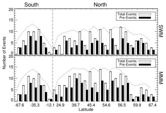
Figure 4.
Latitudinal distribution of weak ionospheric response events for 27 ionosondes. White bars represent the total number of weak response events; black bars show the number of events with pre-storm disturbed geomagnetic conditions.
In the example of Figure 2, where the previous storm appeared to suppress the response to the following storm, the interval between the storms was very short. This can be considered as a special SGS event that is referred to as “SGS-PRE” in this paper. To explore whether this special SGS event can contribute to the weak ionospheric response in the second storm, 21 SGS-PRE events have been further selected with the additional condition that the time interval between the SGS and its preceding geomagnetic storm (Dst < −40 nT) is no more than seven days. The numbers of ionospheric weak response (derived by SWM and MMM) to SGS-PRE events (black bars in Figure 4) are also shown in Figure 4. The weak response to SGS-PRE shows a similar latitudinal trend to the response to SGS.
To explore whether the SGS-PRE can contribute to weak ionospheric response events, the percentages of weak response events that are SGS-PRE events, , and those without a preceding storm, , are calculated and shown in Figure 5. Here, NSGS-PRE is the number of weak ionospheric response events that occur during an SGS-PRE, NSGS is the total number of weak response events, and Nnon-SGS-PRE is the number of weak responses during a non-SGS-PRE. The percentage of weak response events with SGS-PRE is greatly higher than the percentage without SGS-PRE in most stations (>18) for both methods. The latitudinal dependence can be found in the percentage with SGS-PRE. The foF2 storm effect has a seasonal dependence, and the change of ratio and cos χ (where χ is the solar zenith angle) are two important factors responsible for the seasonal variation in the ionospheric F2 layer [25,26].
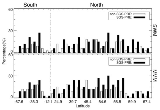
Figure 5.
Latitudinal distribution of ionospheric weak response events with and without super geomagnetic storm with a preceding storm event (SGS-PRE) as a percentage of all super geomagnetic storm (SGS) events. Black (white) bars denote the percentage of ionospheric weak response with (without) SGS-PRE events. The upper panel is the result derived by the spectral whitening method (SWM), and the lower panel is derived by the monthly median method (MMM).
To explore the seasonal variation in the ionospheric weak response, the monthly variation in the number of weak ionospheric response events is studied. As shown in the Figure 6, the number of weak events for 27 ionosondes can be observed in different months. In the SGS events, obvious seasonal dependence can be found in all ionosondes, and the weak response events easily occur in March/April (spring) and September (autumn). Further exploring the SGS-PRE events, the similar seasonal dependence can be also clearly observed. As a result, in the both of storms and preconditioned storms, the weak events occur mainly at the spring and autumn equinox. In March, the number of weak events is same between SGS and SGS-PRE in all stations. However, in the other months, it seems that there are obvious differences between SGS and SGS-PRE in many stations. In general, the number of SGS is larger than that from SGS_PRE. It is a noteworthy that the maximum number of geomagnetic storms is observed precisely during the equinoxes, and it may be small in other moths [24]. In fact, the events of SGS are also maximum during the equinoxes, and the number of SGS events are very few in other months (not shown here). It may result in the maximum of weak ionospheric response to SGS during the equinoxes.
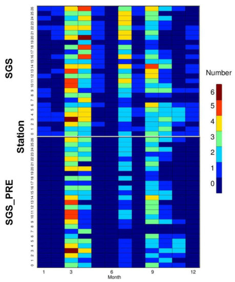
Figure 6.
Seasonal dependence of the number of weak ionospheric response events for 27 ionosondes for SGS events (upper panel) and SGS-PRE events (lower panel).
3.3. Global Results and Analysis
The previous section focused on the regional ionospheric weak response to SGS and SGS-PRE, and we now examine the global ionospheric weak response behavior. The global ionospheric weak response is typically defined by the number of ionosonde stations that show a weak response during a period of SGS. In this paper, the global ionospheric weak response to SGS is specifically defined as more than 75% of the regions (>21 ionosondes) in ionospheric weak response during an SGS. With this definition, SGS events appear mainly during high solar activity (see SGS in Figure 7). The percentages for solar min and solar max in the SGS events derived by SWM show that the ionospheric weak response events occur more frequently in solar max (71.4%) periods than in solar min (14.3%); similarly, in the result derived by MMM, the percentage for solar max (43.8%) is also much higher than that for solar min (12.5%).
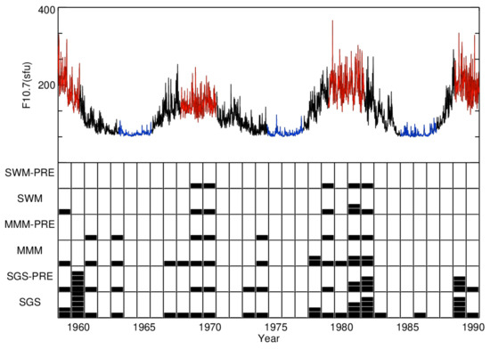
Figure 7.
Daily F10.7 from 1959 to 1990 (upper panel; red and blue denotes solar activity high years and low years respectively) and the number of events each year (lower panel; one black rectangle represents one event). SGS means all super geomagnetic storms (Dst < −200 nT) during the period 1959–1990. Similarly, SGS-PRE means an SGS with a previous geomagnetic storm within no more than seven days. MMM and SWM show the number of ionospheric weak response events to SGS; MMM-PRE and SWM-PRE are the number of ionospheric weak response events to SGS-PRE.
This phenomenon can be observed by both SWM and MMM (lower panel of Figure 7). However, Figure 7 shows that the total number of global weak ionospheric response events derived by SWM (seven events) is critically less than the number of the events derived by MMM (16 events). This is due to the fact that the ionospheric disturbance derived by SWM is more sensitive to geomagnetic activity [7,18], which is difficult to observe at a single station; thus, the results derived by the two methods are similar in Figure 2, but the difference becomes obvious in the global case (Figure 7). In fact, this difference has already been studied by Chen et al. [18], who used the SWM and MMM to construct a global ionospheric index of response to geomagnetic storms. The difference is not clearly shown in the regional ionospheric response (Figure 2) but can be seen in the overall ionospheric behavior (Figure 7). Similarly, the number of weak response events to SGS-PRE with the SWM (five events) is also less than with MMM (eight events). The global weak response with SGS-PRE events as a percentage of all SGS events can be defined as for SWM and for MMM. Here, the NSGS-MMM and NSGS-SWM represent the number of weak response events derived by MMM and SWM during an SGS, respectively. The NSGS-PRE-MMM and NSGS-PRE-SWM are subsets of NSGS-MMM and NSGS-SWM, respectively. They denote weak response events derived by MMM and SWM during an SGS-PRE. With these definitions, the number of global weak response with SGS-PRE events as a percentage of all SGS events is 71.4% and 50% through SWM and MMM, respectively. Although the results vary with method, the percentages suggest that a large proportion of the global ionospheric weak events are SGS-PRE events in both methods.
Our results suggest that SGS-PRE should contributes to global ionospheric weak events, possibly via “long-lasting ionospheric disturbances”. As shown in storm I of Figure 2, a clear ionospheric long-lasting disturbance can be observed over the whole storm event, and even when storm I recovers to the quiet level, ionospheric disturbance can still be found in most stations. When storm II arrives, the ionospheric background may still be in a disturbed state, which can reduce the sensitivity of the ionospheric response to the storm. Therefore, the physical mechanism of long-lasting ionospheric disturbances might play an important role in explaining the ionospheric weak response caused by SGS-PRE. In fact, long-lasting ionospheric disturbance is not a rare phenomenon, and has been extensively studied. Richmond et al. [27] used a coupled magnetosphere–ionosphere–thermosphere model to verify and study long-lasting disturbances, which had been predicted by Fuller-Rowell et al. [1]. Yue et al. [28] also found obvious long-lasting negative ionospheric disturbance during the recovery phase of a super storm. A similar preconditioning effect was also found in a geomagnetic storm event by Lei et al. [29]. Based on these studies and our results, the reduction of the ratio of atomic oxygen to molecular nitrogen (O/N2) might play an important role in long-lasting ionospheric disturbances. The O/N2 ratio is a parameter that strongly determines production and loss in the ionospheric F2 region and the daytime F2 peak density [30]. Therefore, if an ionospheric long-lasting disturbance is caused by a previous geomagnetic storm and the ionosphere is still in a disturbed state, it will be difficult for another intense storm to further change the disturbed (O/N2) significantly, which will result in a weak response in ionospheric peak density or foF2.
The poleward meridional wind disturbance, E × B drift disturbance in the low-latitude ionosphere, and the enhancement of energy (i.e., joule heating) input into the high-latitude ionosphere might also be responsible for the ionospheric weak response. This paper focuses on a preliminary statistical study of the ionospheric weak response, and more advanced physical mechanism studies will be carried out using numerical models in future.
4. Conclusions and Summary
The ionospheric response to a geomagnetic storm is a complex geophysical process. Although a strong geomagnetic storm inputs more energy into the Earth’s upper atmosphere, the ionospheric response often does not reflect the same level of variation as the geomagnetic storm. However, the ionospheric response to geomagnetic activity can vary with the extraction method used. Two different methods, SWM and MMM, are used to explore and verify the statistical characteristics of the regional and global ionospheric weak response to super geomagnetic storms.
In this paper, 27 ionosonde stations in the latitude range 67.4° to −67.6° were selected. During certain geomagnetic storms with geomagnetic index Dst close to −200 nT, the peak value of ionospheric disturbance in most ionosondes remains at a low level, which is almost the same level as before and after the storm. This ionospheric weak response can be observed in the results derived from both SWM and MMM methods, which suggests that this phenomenon is not an artifact of the extraction method but is a real geophysical phenomenon.
Thirty-three SGS events were selected from the period 1959–1990 to statistically analyze the weak ionospheric response to SGS. The results from both methods show that the number of weak ionospheric responses to SGS varies with location, and the regional weak response events occur more frequently in middle latitudes than in high and low latitudes in both hemispheres. To investigate the relationship between SGS-PRE and the weak ionospheric response, the numbers of regional ionospheric weak response events with and without SGS-PRE as a percentage of all SGS events have been calculated. The results derived by the two methods are similar, and the percentage of ionospheric weak response with SGS-PRE events is significantly higher than the percentage without SGS-PRE events in most stations. The global ionospheric weak response has also been examined. The annual numbers of global weak response events to SGS and SGS-PRE were calculated during the period 1959–1990. The results show that the global weak response occurs more frequently under high solar activity than under low solar activity, and results from both methods indicate a high percentage of the number of global weak responses in SGS-PRE events.
In summary, SGS-PRE events are selected to examine whether the effect of one storm on the ionosphere can be influenced by its preconditioning, especially when there is a preceding storm and the time interval between the two storms is short. Our research suggests that (1) for the regional ionosphere, the weak response to SGS shows significant latitudinal and seasonal dependence: it mainly occur in the middle latitudes and appears around equinoxes, the seasonal dependent of weak response to SGS may be because the number of SGS events is maximum around equinoxes; and (2) for the global ionosphere the weak response to SGS occurs more frequently during high solar activity, and the SGS-PRE conditions are shown to contribute to the global ionospheric weak response, which may be related to “long-lasting ionospheric disturbances” [27]. However, the precondition is a very vague description, and it should be a complicated combination of multiple physical factors associated with geomagnetic storms. Therefore, some kind of ionospheric preconditions may contribute to a weak response to geomagnetic storms, but some may not. The precondition should be further classified into different types, and then the more clear relationship between precondition and weak response can be built. However, due to the limitations of observational data, we will plan to explore their clear relationship with more available and different observation in the future work.
Author Contributions
Z.C. developed the basic idea of the paper. H.L. and Z.C. designed the experiments and analysis tools, performed the experiments, and analyzed the data; H.L., L.X., and F.L. participated in discussion and interpretation of the data. H.L. and Z.C. wrote the paper. All authors have read and agreed to the published version of the manuscript.
Funding
This research was funded by the National Natural Science Foundation of China (grants no. 41604136, no. 41604156, no. 41774195, and no. 41974183) and the Natural Science Foundation of Jiangxi Province of China (20171BAB213028).
Acknowledgments
The foF2 data used here are from the Space Physics Interactive Data Resource, online at http://www.ngdc.noaa.gov/stp/spidr.html. The solar F10.7 indices are from the National Geophysical Data Center (NGDC), NOAA, online at https://www.ngdc.noaa.gov/stp/space-weather/solar-data/solar-features/solar-radio/noontime-flux/penticton/. The geomagnetic indices are from the World Data Center for Geomagnetism, Kyoto, online at http://wdc.kugi.kyoto-u.ac.jp/dstae/index.html. We thank the SPIDR, the NGDC, and the World Data Center for Geomagnetism for making their data public. This research was funded by the National Natural Science Foundation of China (grants no. 41604156, no. 41604136, no. 41774195, and no. 41974183).
Conflicts of Interest
The authors declare no conflict of interest.
References
- Fuller-Rowell, T.J.; Codrescu, M.V.; Rishbeth, H.; Moffett, R.J.; Quegan, S. On the seasonal response of the thermosphere and ionosphere to geomagnetic storms. J. Geophys. Res. Space Phys. 1996, 101, 2343–2353. [Google Scholar] [CrossRef]
- Fuller-Rowell, T.M.; Codrescu, M.V.; Roble, R.G.; Richmond, A.D. How does the thermosphere and ionosphere react to a geomagnetic storm? Magn. Storms Geophys. Monogr. Ser. 1997, 98, 203–225. [Google Scholar]
- Prölss, G.W. Magnetic storm associated perturbations of the upper atmosphere. Magn. Storms 1997, 98, 227–241. [Google Scholar]
- Ridley, A.; Deng, Y.; Toth, G. The global ionosphere–thermosphere model. J. Atmos. Sol. Terr. Phys. 2006, 68, 839–864. [Google Scholar] [CrossRef]
- Wang, W.; Lei, J.; Burns, A.G.; Solomon, S.C.; Wiltberger, M.; Xu, J.; Zhang, Y.; Paxton, L.J.; Coster, A. Ionospheric response to the initial phase of geomagnetic storms: Common features. J. Geophys. Res. Space Phys. 2010, 115, A7. [Google Scholar] [CrossRef]
- Mendillo, M. Storms in the ionosphere: Patterns and processes for total electron content. Rev. Geophys. 2006, 44. [Google Scholar] [CrossRef]
- Wang, J.-S.; Chen, Z.; Huang, C.-M. A method to identify aperiodic disturbances in the ionosphere. Ann. Geophys. 2014, 32, 563–569. [Google Scholar] [CrossRef]
- Mednikova, N.B. Mid-Latitude Ionospheric Disturbances. In Physics of Solar Corpuscular Fluxes and Their Impact on the Upper Atmosphere of the Earth; Academic Press of USSR: Moscow, Russia, 1957; p. 183. (In Russian) [Google Scholar]
- Radicella, S.; Zhang, M.-L.; Romanelli, L.; Figliola, A. A critical analysis of monthly medians and variability of ionospheric parameters. Adv. Space Res. 1995, 15, 45–50. [Google Scholar] [CrossRef]
- Kouris, S.; Fotiadis, D. Ionospheric variability: A comparative statistical study. Adv. Space Res. 2002, 29, 977–985. [Google Scholar] [CrossRef]
- Mikhailov, A.V.; Depueva, A.K.; Leschinskaya, T.Y. Morphology of quiet time F2-layer disturbances: High to lower latitudes. Int. J. Geomagn. Aeron. 2004, 5, GI1006. [Google Scholar] [CrossRef]
- Jakowski, N.; Stankov, S.; Schlueter, S.; Klaehn, D. On developing a new ionospheric perturbation index for space weather operations. Adv. Space Res. 2006, 38, 2596–2600. [Google Scholar] [CrossRef]
- Gulyaeva, T.L.; Stanislawska, I. Derivation of a planetary ionospheric storm index. Ann. Geophys. 2008, 26, 2645–2648. [Google Scholar] [CrossRef]
- Depueva, A.K.; Mikhailov, A.V.; Depuev, V.K. Quiet timeF2–layer disturbances at geomagnetic equator. Int. J. Geomagn. Aeron. 2005, 5, GI3001. [Google Scholar] [CrossRef]
- Mikhailov, A.V.; Depueva, A.H.; Depuev, V.H. Daytime F2-layer negative storm effect: What is the difference between storm-induced and Q-disturbance events? Ann. Geophys. 2007, 25, 1531–1541. [Google Scholar] [CrossRef]
- Chen, Z.; Jin, M.; Deng, Y.; Wang, J.-S.; Huang, H.; Deng, X.; Huang, C.M. Improvement of a deep learning algorithm for total electron content maps: Image completion. J. Geophys. Res. Space Phys. 2019, 124, 790–800. [Google Scholar] [CrossRef]
- Tang, R.; Zeng, F.; Chen, Z.; Wang, J.-S.; Huang, C.-M.; Wu, Z. The comparison of predicting storm-time ionospheric TEC by three methods: ARIMA, LSTM, and Seq2Seq. Atmosphere 2020, 11, 316. [Google Scholar] [CrossRef]
- Chen, Z.; Wang, J.; Huang, C.M.; Huang, L. A new pair of indices to describe the relationship between ionospheric disturbances and geomagnetic activity. J. Geophys. Res. Space Phys. 2014, 119. [Google Scholar] [CrossRef]
- Chen, Z.; Wang, J.-S.; Deng, X.; Deng, Y.; Huang, C.M.; Li, H.M.; Wu, Z.X. Study on the relationship between the residual 27 day quasiperiodicity and ionospheric Q disturbances. J. Geophys. Res. Space Phys. 2017, 122, 2542–2550. [Google Scholar] [CrossRef]
- Chen, Z.; Wang, J.-S.; Deng, Y.; Huang, C.-M. Extraction of the geomagnetic activity effect from TEC data: A comparison between the spectral whitening method and 28 day running median. J. Geophys. Res. Space Phys. 2017, 122, 3632–3639. [Google Scholar] [CrossRef]
- Blanc, M.; Richmond, A. The ionospheric disturbance dynamo. J. Geophys. Res. Space Phys. 1980, 85, 1669–1686. [Google Scholar] [CrossRef]
- Foster, J.C.; Maurice, J.P.S.; Abreu, V.J. Joule heating at high latitudes. J. Geophys. Res. Space Phys. 1983, 88, 4885–4897. [Google Scholar] [CrossRef]
- Rishbeth, H.; Fuller-Rowell, T.J.; Rodger, A.S. F-layer storms and thermospheric composition. Phys. Scr. 1987, 36, 327–336. [Google Scholar] [CrossRef]
- Gonzalez, W.D.; Joselyn, J.A.; Kamide, Y.; Kroehl, H.W.; Rostoker, G.; Tsurutani, B.T.; Vasyliunas, V.M. What is a geomagnetic storm? J. Geophys. Res. Space Phys. 1994, 99, 5771–5792. [Google Scholar] [CrossRef]
- Millward, G.H.; Rishbeth, H.; Fuller-Rowell, T.J.; Aylward, A.D.; Quegan, S.; Moffett, R.J. Ionospheric F2 layer seasonal and semiannual variations. J. Geophys. Res. Space Phys. 1996, 101, 5149–5156. [Google Scholar] [CrossRef]
- Rishbeth, H.; Mendillo, M. Patterns of F2-layer variability. J. Atmos. Sol. Terr. Phys. 2001, 63, 1661–1680. [Google Scholar] [CrossRef]
- Richmond, A.; Peymirat, C.; Roble, R.G. Long-lasting disturbances in the equatorial ionospheric electric field simulated with a coupled magnetosphere-ionosphere-thermosphere model. J. Geophys. Res. Space Phys. 2003, 108. [Google Scholar] [CrossRef]
- Yue, X.; Wang, W.; Lei, J.; Burns, A.; Zhang, Y.; Wan, W.; Liu, L.; Hu, L.; Zhao, B.; Schreiner, W.S. Long-lasting negative ionospheric storm effects in low and middle latitudes during the recovery phase of the 17 March 2013 geomagnetic storm. J. Geophys. Res. Space Phys. 2016, 121, 9234–9249. [Google Scholar] [CrossRef]
- Lei, J.; Thayer, J.P.; Burns, A.G.; Lu, G.; Deng, Y. Wind and temperature effects on thermosphere mass density response to the November 2004 geomagnetic storm. J. Geophys. Res. Space Phys. 2010, 115. [Google Scholar] [CrossRef]
- Rishbeth, H. How the thermospheric circulation affects the ionospheric F2-layer. J. Atmos. Sol. Terr. Phys. 1998, 60, 1385–1402. [Google Scholar] [CrossRef]


© 2020 by the authors. Licensee MDPI, Basel, Switzerland. This article is an open access article distributed under the terms and conditions of the Creative Commons Attribution (CC BY) license (http://creativecommons.org/licenses/by/4.0/).